Article

Applied Machine Learning for Geometallurgical Throughput Prediction—A Case Study Using Production Data at the Tropicana Gold Mining Complex

by
Christian Both
* and
Roussos Dimitrakopoulos
*
COSMO—Stochastic Mine Planning Laboratory, Department of Mining and Materials Engineering, McGill University, 3450 University Street, Montreal, QC H3A 0E8, Canada
*
Authors to whom correspondence should be addressed.
Minerals 2021, 11(11), 1257; https://doi.org/10.3390/min11111257
Submission received: 11 October 2021 / Revised: 2 November 2021 / Accepted: 10 November 2021 / Published: 12 November 2021

Abstract

:
With the increased use of digital technologies in the mining industry, the amount of centrally stored production data is continuously growing. However, datasets in mines and processing plants are not fully utilized to build links between extracted materials and metallurgical plant performances. This article shows a case study at the Tropicana Gold mining complex that utilizes penetration rates from blasthole drilling and measurements of the comminution circuit to construct a data-driven, geometallurgical throughput prediction model of the ball mill. Several improvements over a previous publication are shown. First, the recorded power draw, feed particle and product particle size are newly considered. Second, a machine learning model in the form of a neural network is used and compared to a linear model. The article also shows that hardness proportions perform 6.3% better than averages of penetration rates for throughput prediction, underlining the importance of compositional approaches for non-additive geometallurgical variables. When adding ball mill power and product particle size, the prediction error (RMSE) decreases by another 10.6%. This result can only be achieved with the neural network, whereas the linear regression shows improvements of 4.2%. Finally, it is discussed how the throughput prediction model can be integrated into production scheduling.

1. Introduction

In recent years, the amount of collected and centrally stored production data in the mining industry has increased massively with the implementation of digital technologies. Some examples of centrally stored datasets in operating mines are records of fleet management systems [1], measurement while drilling (MWD) [2], measurements of material characteristics using sensor techniques [3], and other key performance indicators at the processing plants. While potentially all mine planning activities can benefit from the analysis of production data (data analytics), interdisciplinary fields such as geometallurgy can particularly gain from this growing data. Geometallurgy aims to capture the relationships between spatially distributed rock characteristics and its metallurgical behavior when the mined materials are processed and transformed into sellable products. One pertinent part of geometallurgy is the optimization of comminution circuits and the prediction of comminution performance indicators such as throughput in the mineral processing facilities [4,5,6]. However, value is only added to the operation when the gained geometallurgical knowledge is integrated into decision-making processes, whereas appropriate methods are still mostly lacking for the tactical or short-term production planning horizon [7]. Another current limitation is the cost-intensive sampling and laboratory testing of rock hardness and grindability [8]. The present article shows a case study at the Tropicana Gold mining complex that demonstrates how production data combined with machine learning can be used to construct a data-driven geometallurgical throughput prediction model and how such a model can subsequently be utilized for short-term mine production scheduling.
The optimization of comminution circuits has traditionally relied on well-accepted comminution laws and ore hardness and grindability indices for ball/rod mills [9,10] and SAG mills [11,12,13]. These comminution models are routinely used for optimized grinding circuit design, using averages or ranges of ore hardness tests of the mineral deposits to be extracted. Instead of using constant values representing whole deposits, geometallurgical programs account for the heterogeneity of geometallurgical variables within the mineral reserve and their effect on downstream processes over time [14]. A typical geometallurgical workflow includes a spatial model, which comprises geostatistically simulated or estimated variables (e.g., grindability). Several case studies have demonstrated how throughput rates of a comminution circuit can be predicted using spatial geometallurgical models of hardness and grindability indices in combination with comminution theory [15,16,17,18]. Although some of these throughput models have demonstrated high accuracy in reconciliation studies, there are notable challenges when using and integrating them into decision-making processes such as short-term production scheduling. First, the geometallurgical sampling program requires cost-intensive laboratory testing to obtain the abovementioned hardness and grindability indices [8,13]. The high associated costs spent in early project stages can be prohibitively large and typically result in very sparse sampling, although research is being conducted to increase the number of samples by using alternate data measurement tools and small-scale processing tests [19]. Second, the throughput prediction models are built to evaluate the weekly or monthly performance of mine production schedules a posteriori, instead of integrating them into short-term production scheduling. Third, none of the models account for the inherent uncertainty of the geometallurgical variables stemming from the imperfect knowledge of the orebody.
There have been efforts to incorporate geometallurgical hardness properties and their associated geological uncertainty into mine production scheduling in single, open-pit mines [20] and in mining complexes [21]. The stochastic optimization models are developed for long-term production scheduling and require that hardness and grindability indices are geostatistically simulated for volumes of selective mining units (mining block). However, most of the frequently utilized hardness and grindability indices are non-additive [13,22,23]. Geometallurgical samples are also collected on large support scales [24,25] and are typically very sparse, as mentioned earlier. These complicating factors make the joint spatial interpolation of geometallurgical variables and their change of support from point measurements to mining blocks challenging [25,26,27,28]. Morales et al. [20] optimize the mine production schedule using precalculated mill throughputs and economic values for each block independently. The method thus ignores that extracted materials are blended in stockpiles and in processing facilities; consequently, the non-additive comminution behavior of blended materials and resulting metal production cannot be correctly assessed. Kumar and Dimitrakopoulos [29] optimize a mining complex while including predefined ratios of hard and soft rock, to achieve a consistent throughput in processing streams. However, these ratios are defined arbitrarily, and details of short-term planning are not addressed.
Both and Dimitrakopoulos [30] present a new approach that integrates a geometallurgical throughput prediction model into short-term stochastic production scheduling for mining complexes. The stochastic production-scheduling formulation builds upon simultaneous stochastic optimization of mining complexes [31,32] which optimizes pertinent components of a mining complex in a single mathematical model and incorporates geological uncertainty to minimize technical risk. Instead of using block throughput rates, the production-scheduling formulation calculates the throughput of blended materials using an empirically created throughput prediction model, learning from previously observed throughput rates at the ball mill [30]. One limitation of this work is that the integrated throughput prediction model so far has only considered rock hardness, density, lithology, and weathering degree of the mineral reserve. This ignores that mill throughput rates also depend on operating factors of the processing plant, such as power draw, utilization rates, and particle size distributions. Second, a multiple linear regression (MLR) has been used for throughput predictions, which is unable to capture potential nonlinear relationships among input variables and geometallurgical response.
The case study at the Tropicana Gold mining complex shown in this article expands the method presented in Both and Dimitrakopoulos [30] in multiple ways. First, the recorded plant measurements power draw, feed particle size, and product particle size of the ball mill are newly considered to improve the prediction of ball mill throughput rates. Second, a more powerful supervised learning method in the form of an artificial neural network is tested and compared to MLR, since the addition of the new comminution-related features increases the possibilities of nonlinear interactions between predictive and response variables. The plant measurements, including the observed ball mill throughput, are retrieved from the comminution circuit at the Tropicana Gold mining complex. The other dataset used in this case study to predict ball mill throughput comprises penetration rates from measurement while drilling (MWD). The use of this dataset is motivated by its ability to indicate the strength and hardness of the intact rock [2,33,34]. The penetration rates are converted into a set of hardness proportions per selective mining unit (SMU) which has recently been proposed to build a link between intact rock hardness and comminution performance of the rock in milling and grinding circuits [30]. The present article also compares the prediction capabilities of hardness proportions to averages of penetration rates. In this way, the effect of ignoring non-additivity of hardness-related geometallurgical variables can be quantified, an issue that has had little attention in the literature thus far.
In the following sections, the components of the Tropicana Gold mining complex are introduced first, together with all utilized production data that are used for the prediction of ball mill throughput. The supervised machine learning model is discussed next, including a statistical analysis of the present dataset and a hyperparameter calibration. Analysis of results, discussion, and conclusions follow.

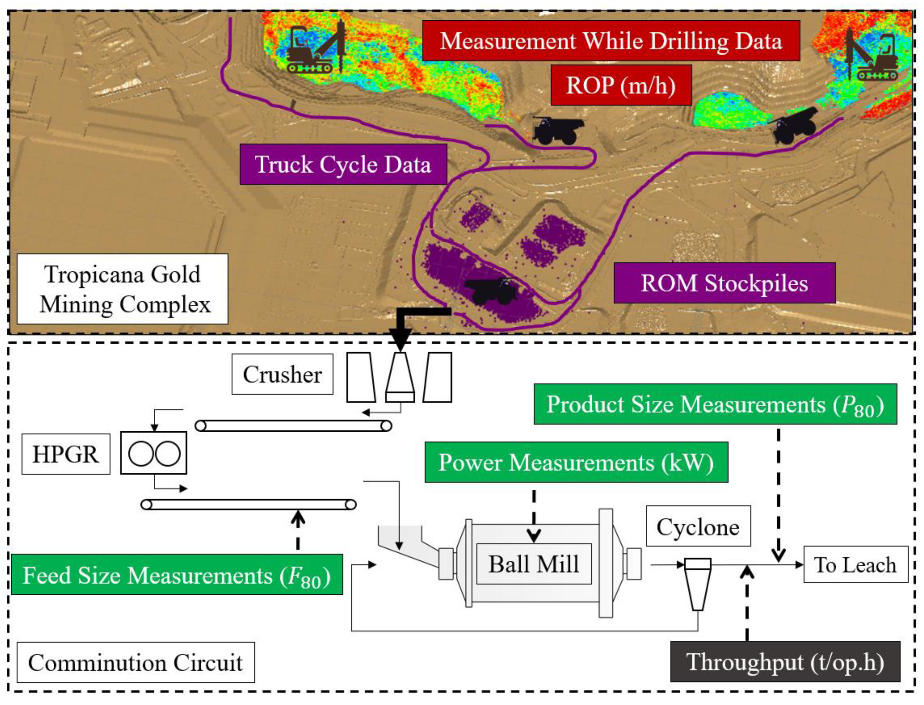
2. The Tropicana Gold Mining Complex and Utilized Production Data for Ball Mill Throughput Prediction

The Tropicana Gold mining complex is located in western Australia in the west of the Great Victoria Desert. The gold deposit is mined from four pits, Boston Shaker, Tropicana, Havana, and Havana South (from north to south), as can be seen in the aerial view in Figure 1. In addition, the mining complex contains a processing plant, stockpiles, a tailings facility, and multiple waste dumps. Gold is produced onsite in a single processing stream, consisting of a comminution circuit and a carbon-in-leach (CIL) plant.
The displayed dataset in the four pits in Figure 1 shows the drilling rate of penetration (ROP) from production drilling (blastholes), which is part of the measurement while drilling (MWD) dataset collected at the Tropicana Gold mining complex. It is clearly visible how ROP reflects the heterogeneity of the rock and decreases with depth. Exemplary, easy-to-drill (softer) rock is found towards the surface (red colors at Havana South Pit and Boston Shaker Pit), whereas difficult-to-drill (harder) rock is located deeper in the pits (green–blue colors in Havana Pit, Tropicana Pit, and deeper cutback of Boston Shaker Pit). Both and Dimitrakopoulos [30] demonstrate strong correlations between the rate of penetration (ROP) of drilled rock and ball mill throughput when these rock parcels are sent to the processing plant. They subsequently present a method that predicts ball mill throughput using ROP. This article extends this work by utilizing additional measurements in the processing plant related to ball mill throughput.
The relevant material flow in the mining complex is shown together with all utilized production data in Figure 2. Detailed material tracking in daily intervals is performed using truck cycle data, starting from the material extraction in the pits and ending at the crusher. Crucially, material tracking includes all dumping and rehandling activities at run-of-mine (ROM) stockpiles, since rehandled material accounts for 80–90% of processed ore in the Tropicana Gold mining complex. In this way, ROP entries recorded in the pits can be successfully linked to observed measurements in the processing plant, including the observed throughput of the ball mill. Details of successful implementations of material tracking that include stockpiles can be found in Wambeke et al. [35] and Both and Dimitrakopoulos [30].
The comminution circuit at Tropicana Gold mining complex comprises three stages: crushing (primary and secondary crusher), grinding (high-pressure grinding roll, HPGR), and milling (ball mill). The cyclone overflow is sent to the CIL plant to extract the gold. The recorded average power draw of the ball mill and the particle size distributions entering and leaving the ball mill are of particular interest for throughput prediction. Note that the feed and product particle size distributions are subsequently defined by their 80% passing diameters in μm. The feed particle size measurements ( F 80 ) are performed using image analyzers on the conveyor belt of the HPGR product. Shift composites of cyclone overflow samples are used for product particle size measurements ( P 80 ).
The relevance of all presented measurements above can be derived from comminution theory, such as Bond’s law of comminution [9,10]. The Bond equation (Equation (1)) calculates the specific energy of the ball mill ( W in kWh/t) required to grind the ore from a known feed size ( F 80 ) to a required product size ( P 80 ).
W = W i * ( 10 P 80 10 F 80 )
The Work index (Wi in kWh/t) is a measure of the ore’s resistance to crushing and grinding [9]. In this article, it is useful to substitute the specific energy of the ball mill (energy delivered per ton of ore in kWh/t) by the quotient of mill power draw (kW) and mill throughput (processed tons per operating hour), as shown in Equation (2).
P o w e r   T P H   = W i * ( 10 P 80 10 F 80 )
Equation (3) is obtained by rearranging Equation (2) for ball mill throughput (TPH).
T P H = P o w e r W i * ( 10 P 80 10 F 80 )
Next to the measured power draw and particle size distributions, it is clear that throughput predictions of the ball mill must include some kind of information about ore hardness. Generally, the harder the material, the higher its resistance against comminution, thus needing to reside longer in the ball mill to reach the desired product size, given constant power draw and particle feed size. In Bond’s equation, TPH is inversely proportional to W i , as shown in Equation (4).
T P H 1 W i
As introduced above, the role of informing ore hardness is taken over by ROP measurements in this article. By utilizing cost-effective and easily accessible production data (MWD information generated by drilling machines), costly and time-consuming laboratory tests spent for W i estimates of the geological reserve can be replaced. Mwanga et al. [8] report that the typical sample volume required for Bond tests is relatively large (2–10 kg, depending on test modification), and requires crushed ore smaller than 3.35 mm (passing a 6-mesh sieve). Furthermore, several grinding cycles are necessary to reach the steady state of the simulated closed circuit. The alternative utilization of ROP is especially promising as a substitute for W i because of its demonstrated ability to indicate rock type, strength, and alteration [34,36,37,38]. In general, high ROP (in m/h) indicates less competent rock, bearing lower W i . In turn, TPH is expected to increase, as shown in Equation (5).
R O P   ( m h )     W i   ( k W h t )     T P H  
Note that the dependencies in Equation (5) may be nonlinear. Rather, potentially nonlinear dependencies call for more sophisticated prediction models for TPH prediction, which are subsequently discussed in Section 3.

3. Application of Supervised Machine Learning for Throughput Prediction

This section discusses the use of supervised machine learning to create a throughput-prediction model at the Tropicana Gold mining complex. Supervised machine learning models require labelled datasets for training, consisting of data pairs { x i ,   y i },   i = 1 , , N , whereas x i is a vector of predictor variables, and y i   is the known response. In this article, the known response (label) is the observed ball mill throughput, and the M predictor variables (features) comprise of the geological attributes of the ore and measured variables in the comminution circuit. Throughput responses are recorded on a continuous scale, rendering the supervised learning problem a regression task ( y i   ).

3.1. Neural Networks

A feed-forward neural network is chosen as a supervised learning model for the potentially nonlinear task of ball mill throughput prediction. In its essence, feed-forward neural networks are fully connected, layered combinations of neurons that find their origins in the perceptron model [39]. A single neuron (perceptron) calculates the inner product between its internal weight vector, w T , and the input vector, x. After adding a bias term, b , the resulting value is passed through a nonlinear activation function, g (   ·   ) , creating a scalar output z = g ( w T x + b ) . Several connected neurons to x form the so-called first hidden layer of the neural network. If the outputs of the first hidden layer are passed through another layer of neurons, a multilayer neural network is built [40]. The output layer comprises a single neuron that receives as input the vector of hidden outputs, z , and provides an estimate, y ^ . Neural networks are the method of choice in this article because they have the proven advantage of being capable of approximating every arbitrary function using either one hidden layer of exponentially many neurons, or multiple consecutive neural layers consisting of fewer neurons [41]. This gives neural networks theoretical advantages over linear prediction models, such as multiple linear regression, which has been tested in previous work for throughput prediction [30]. Univariate statistics and correlations in the present dataset, including potential nonlinearities, are discussed next, followed by the discussion of the utilized neural network architecture, and tuning of its hyperparameters.

3.2. Dataset and Statistical Analysis

The dataset for throughput prediction contains the hardness-related rate of penetration (ROP) of the ore, which has been tracked in the Tropicana Gold mining complex, as presented in Figure 2. The power draw, F 80 , and P 80 measurements, as well as a ball mill utilization factor reflecting ball mill up- and down-time, are also included. A 7-day moving average of the data is calculated for an observed time horizon of six months (February–August 2018), which reduces noise in the dataset and helps recognize trends of higher and lower throughput rates that are more likely connected to rock properties of the material processed. In the six-month interval, extraction mainly occurs in two pits, the Tropicana and Havana Pit, and material is continuously stockpiled at the ROM stockpiles. Univariate statistics of the predictive variables and the response variable (throughput) are shown in Table 1.
Table 2 shows linear correlations between pertinent features and observed TPH using Pearson’s correlation coefficient, in Equation (6) below, with x i and y i representing individual sample points and x ¯ ,   y ¯ indicating sample means. Note that correlations in Table 2 can be inflated because they are calculated after applying the moving average.
r = i = 1 n ( x i x ¯ ) ( y i y ¯ ) i = 1 n ( x i x ¯ ) 2 * i = 1 n ( y i y ¯ ) 2
The tracked ROP entries are henceforth used in two different ways to inform material hardness. The feature ‘Average ROP’ comprises weighted averages of continuous ROP values linked to the materials that are transported to the crusher in the same observed time interval. In contrast, Both and Dimitrakopoulos [30] propose a compositional approach, which partitions ROP into easier-to-drill (softer rock) and difficult-to-drill (harder rock) categories, using a set of ROP intervals. The split in multiple intervals results in proportions of harder or softer materials sent to the comminution circuit in a given time interval. A detailed explanation of how to calculate these hardness proportions is given in Both and Dimitrakopoulos [30]. The listed features in Table 2 can broadly be distinguished into three categories, whereas the first two categories are related to ore hardness. Average ROP comprises the first category (A1), and hardness proportions built by intervals of penetration rates comprise the second category (B1–B10). The third feature category reflects measurements at the comminution circuit (C1–C4).
By comparing the Pearson correlation coefficients in Table 2, it can be seen that some variables correlate more strongly with TPH, whereas other variables do not. A stronger positive correlation of TPH for ‘Average ROP’ (in m/h) gives the first evidence of the usefulness of this feature (A1). The compositional approach effectively partitions the distribution of penetration rates into multiple hardness categories. Here, a higher percentage of difficult-to-penetrate material in the processed ore blend (B1–B6) indicates harder material, thus lowering TPH, which is confirmed by the negative correlation in Table 2. Conversely, a higher fraction of easier-to-penetrate material in the blend is expected to increase TPH, which is equally confirmed in Table 2 through positive correlations of categories B8–B10. Interestingly, some hardness categories show a stronger correlation (positive and negative) than the average ROP feature (A1). This indicates that additional information may be conveyed through the creation of hardness categories. The prediction potential of average penetration rates and hardness proportions is compared in detail in Section 4.1.
According to Equation (5), the relationship between ball mill power and TPH is directly proportional. This theoretical relationship is empirically well reflected in Table 2, showing a stronger positive correlation between ball mill power (C3) and TPH. The power measurements thus comprise an important part of throughput prediction, subsequently performed in Section 4 of this article. Although the ball mill utilization (C4) is not part of Bond’s equation, it is not surprising to see a stronger correlation to TPH. Events of planned and unplanned ball mill downtime, i.e., utilization < 100 percent, ramp-up and ramp-down processes, are among the effects that also lower the effective throughput per operating hour. A redundancy between ball mill utilization and ball mill power is observed, confirmed by similar statistics of power and utilization in Table 1, which explains similar correlation in Table 2. Relationships between TPH and particle sizes of the ore that result from Bond’s law (Equation (1)) are shown in Equations (7) and (8).
P 80       T P H  
F 80       T P H  
On the one hand, a coarser product particle size (larger P 80 value) results in higher TPH (Equation (7)), given that ore characteristics, energy input and feed particle size stay the same. On the other hand, a finer-grained feed size (smaller F 80 value) can also lead to an increased TPH because less grinding work needs to be applied to reach the desired product size (Equation (8)). In the present dataset, the particle size measurements (C1–C2) show very little correlation in Table 2. This can be for several reasons. Contrary to power draw, the relationships in Equations (7) and (8) are nonlinear, and the particle size measurements are incomplete for some periods, as indicated in Table 1. Additionally, one must consider that particle size measurements over running belts are error-prone, especially when using image analyzers for F 80 . It is analyzed in Section 4 whether particle size measurements can enhance throughput prediction in practice. Note that all comminution variables are scaled before usage by dividing by their maximum value. Compositional data naturally comprises fractional values in [0,1] and thus does not have to be scaled.

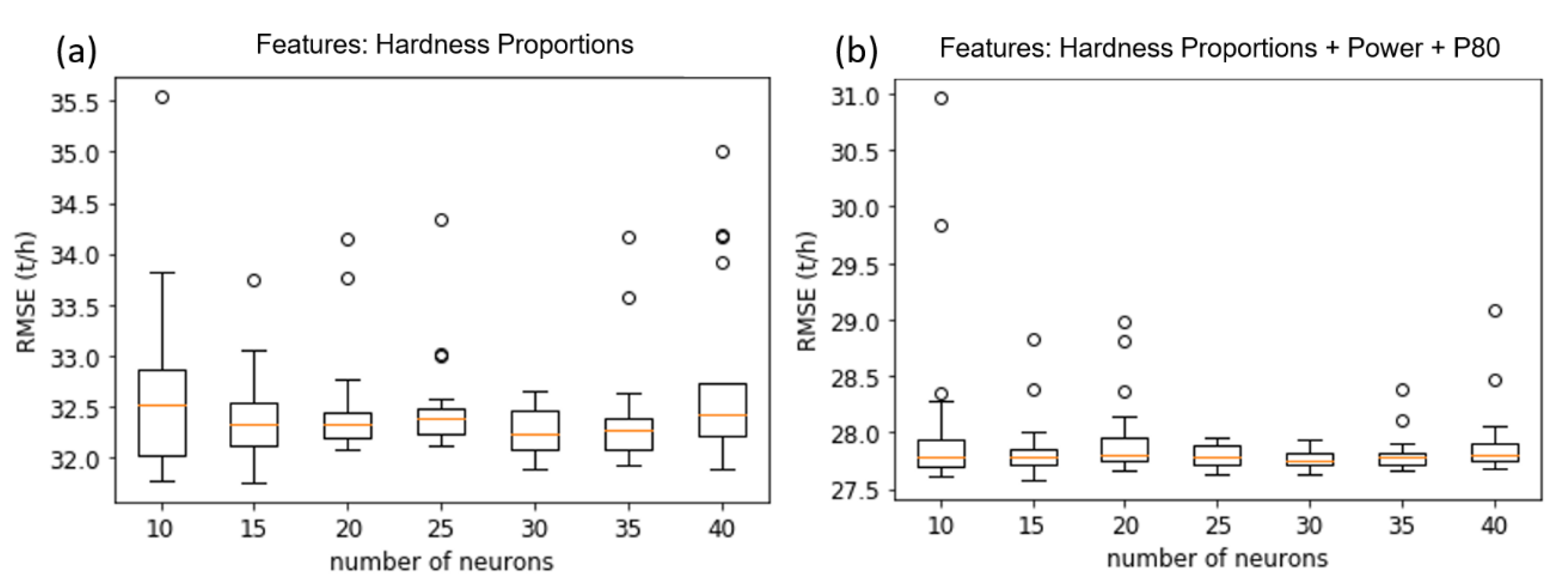
3.3. Network Architecture and Hyperparameter Search

In its implementation, the architecture of a feed-forward neural network requires the calibration of several hyperparameters. The hyperparameter setting is relevant to the evaluation process and robustness of the approach. Therefore, it becomes obvious to explore the hyperparameter space in order to find a stable region of this space [42]. However, due to the small size of the dataset (181 data points) and the need to test on the entire horizon (181 days) to extrapolate the overall performance of the proposed approach, the dataset cannot be split. Instead, k-fold cross-validation is used to measure the configuration quality, thus minimizing the information loss [43]. Different periods are used for different folds (20 folds) to simulate the more realistic scenario where a prediction is made over a new period. The network architecture is implemented in Python using the scikit-learn package [44]. The squared error between the observed throughput, y i ,   i = 1 , , N , and predicted throughput, y ^ i ,   i = 1 , , N , is chosen as the loss function to be minimized during training, and the rectified linear unit is chosen as activation function. The quasi-Newtonian L-BFGS algorithm [45] is used to minimize the loss function, which proved to converge more quickly on the small dataset compared to stochastic gradient methods. Finally, the root-mean-squared error (RMSE) is used for comparisons.
Early stopping of training is important to prevent overfitting in neural networks, and therefore, the number of training iterations is a hyperparameter that needs to be calibrated [46]. It was found that the validation error was minimal after five iterations. L2 regularization was tested but did not significantly increase generalization potential in this application.

Number of Layers and Neurons

Figure 3 shows a sensitivity analysis of the number of neurons for two selected feature sets. In Figure 3a, only hardness-related features are used, whereas Figure 3b includes more features. Given the stochastic processes involved during training, each network configuration is repeated 20 times using random initializations of weights. This procedure results in a sample of errors that are shown by boxplots.
Figure 3 shows that the average error and error variance reduce for both feature sets as the number of neurons increases. A plateau is reached at 25 to 30 neurons. This is expected since a too small number of neurons is not able to adequately map the underlying function. Note that this behavior can be observed independently of the number of layers. Two fully connected hidden layers are used in Figure 3a, whereas a single connected hidden layer was used for the sensitivity analysis in Figure 3b. For the best choice of layers, another sensitivity analysis is performed by varying the number of hidden layers from one to four. Figure 4 shows the results performed on the same selected feature sets.
Figure 4 indicates that one hidden layer delivers the most stable results on all tested feature sets. Although the addition of more layers can reduce the error in individual runs, as seen in Figure 4a, the network appears more prone to overfitting and the error variance increases. For larger feature sets (Figure 4b), overfitting appears to be exacerbated the more layers are used. The obtained results demonstrate the strength of parsimony of parameters (POP), as the model with the smallest size (i.e., one hidden layer) performs best.

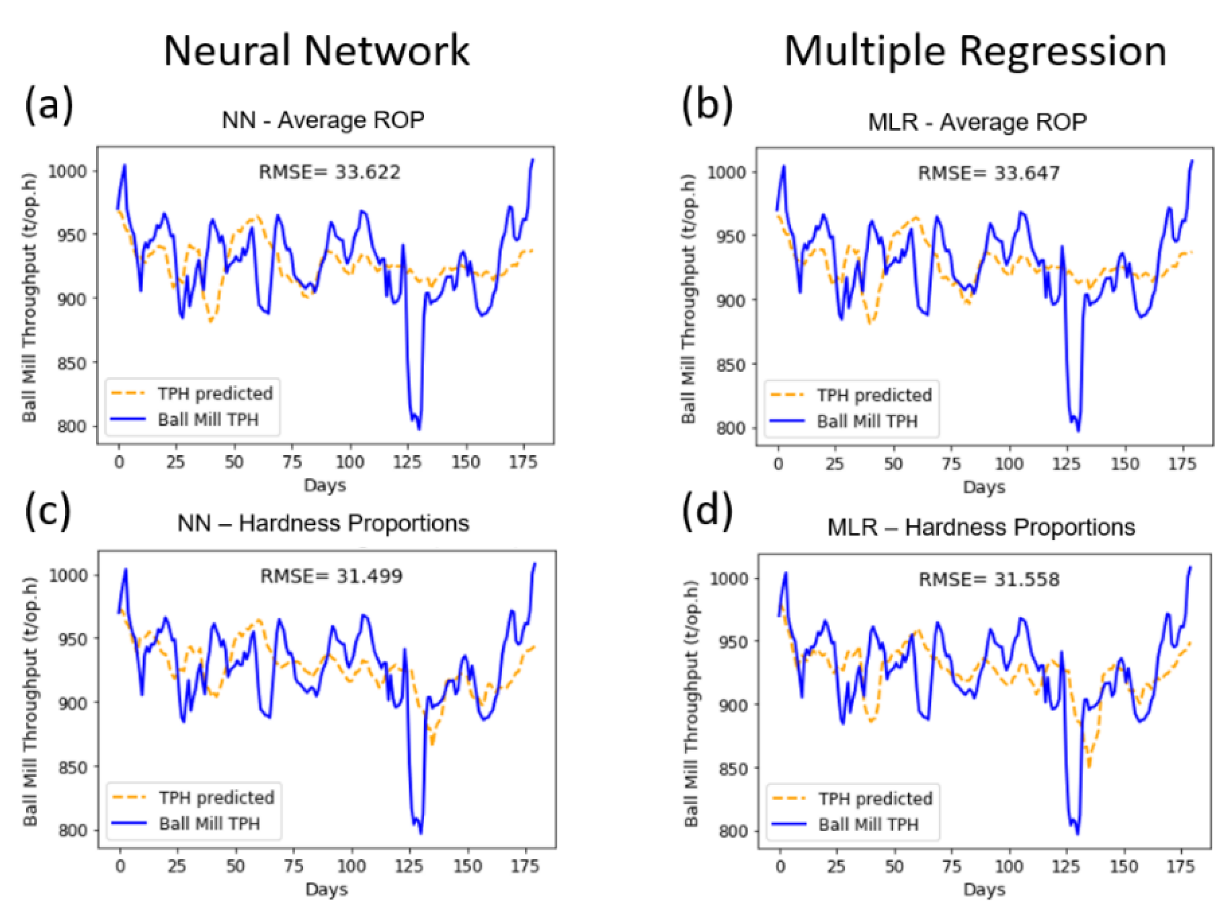
4. Results and Analysis

Section 4 is subdivided into two separate parts that aim to analyze the effects of different feature sets on throughput prediction, and then benchmark the presented neural network against a multiple regression model. Section 4.1 addresses the prediction of ball mill throughput using hardness-related variables only. In Section 4.2, pertinent comminution variables are added individually, and their effect on throughput prediction is evaluated.

4.1. Hardness-Related Variables (Effect of Non-Additivity)

This subsection aims to answer how different ways of informing about the hardness and grindability of the geological reserve using penetration rates from blasthole drilling perform for throughput prediction. Specifically, the prediction potential of the average rate of penetration (ROP) is compared to the prediction behavior of hardness proportions created using penetration rate intervals. Figure 5a shows a graphical comparison of ball mill throughput (left axis) and average ROP of the processed ore (right axis). Figure 5b,c illustrates the evolution in time of two distinct hardness proportions compared to throughput, and are discussed subsequently.
It can be seen in Figure 5a that average ROP follows ball mill throughput well in many periods of the observed time horizon. Together with the strong positive correlation reported in Table 2, the similar behavior of both variables in Figure 5a confirms the hypothesis that penetration rates recorded by drilling machines can contribute to informing the comminution performance and grindability of the processed ore. Next, this feature is tested using 20-fold cross-validation. The performance of average ROP as a single feature for throughput prediction is shown in Figure 6a (neural network) and Figure 6b (multiple regression).
When comparing Figure 6a,b, there appears to be no obvious advantages of the neural network compared to multiple regression, which can be explained by the fact that only one single feature is used. Although following the general trends of throughput in most of the observed time intervals, the results reveal weaknesses in predicting the right magnitudes of low and high throughputs. A possible explanation for this weakness can be found when considering penetration rates as a non-additive variable. Non-additivity is present if linear averages of a variable, for instance penetration rates of two separate rock entities, are different from the expected value of the combined (blended) sample. Thus, taking mathematical averages can be detrimental to such variables. Other well-known examples are metal recovery [47] and other variables representing product quality [48].
In fact, the feature ‘average ROP’ has gone through an averaging process twice. First, penetration rates are averaged within a mining block when changing the support from simulated grid nodes (point support) to mineable volumes (SMU) to reflect mine selectivity. This standard process is only innocuous for additive variables such as metal grades (at constant density). Second, a weighted average by tonnage of each truckload is calculated per day, accounting for all sources of material that are blended. For the alternative feature set of hardness proportions, penetration rates in point support are split into several categories using penetration rate intervals. This procedure avoids the averaging of harder and softer parts within the geological reserve. Instead, proportions of softer and harder material are preserved in the ore blends that are processed in the mill (compositional approach). A discussion of how to build hardness proportions and how many hardness categories are needed can be found in Both and Dimitrakopoulos [30].
Figure 5b,c illustrates the evolution of two distinct hardness proportions compared to TPH. Figure 5b shows the proportions of soft material arriving at the mill, informed by the percentage of high penetration rates (greater than 62 m/h) in the ore blend. Here, higher throughputs are expected to occur when more of this soft material arrives at the mill. Indeed, large proportions of softer material in Figure 5b coincide with high mill throughput, which is most visible for days 1–10 as well as for days 170–181 of the observed period. Figure 5c shows the proportions of harder material, which is reflected by penetration rates that fall in the interval of 29 to 32 m/h. Larger proportions of this material category should have a negative effect on throughput. Interestingly, Figure 5c shows that the lowest mill throughput (days 128–133) coincides with the peaking of the fractions of harder material. Conversely, the highest throughput is achieved when the proportions of this harder-to-penetrate material are the smallest.
The performance of hardness proportions for throughput prediction is shown in Figure 6c (neural network) and Figure 6d (multiple regression). The highs and lows of throughput are more closely predicted, leading to a reduction in the prediction error by 6.3% for both prediction models. This indicates that classification into hardness proportions is advantageous over using a single, continuous hardness variable. The difference between the neural network and the multiple regression model is relatively small.

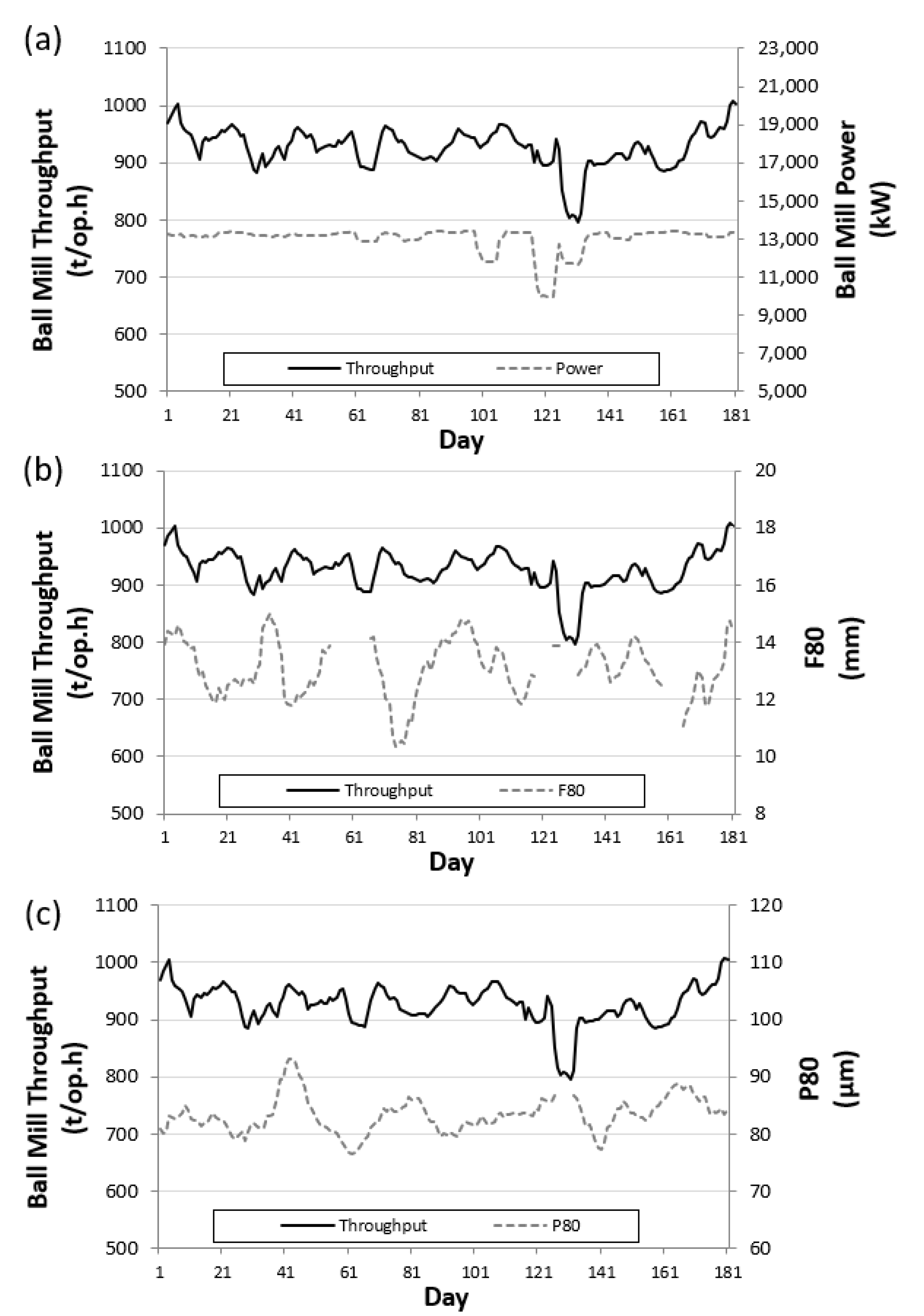
4.2. Effect of Comminution Variables on Prediction

Several comminution variables were identified as potential candidates to improve throughput prediction in Section 2 and Section 3. In this subsection, the hardness feature set comprising hardness categories is enhanced by one additional comminution variable at a time. To analyze the effects of the neural network, a comparison to a multiple linear regression model is provided for each experiment.

4.2.1. Ball Mill Power

The ball mill power measurements showed the potential to improve the prediction of ball mill throughput due to its proportional relationship to TPH in Bond’s law (Equation (1)) and its strong correlation in the present dataset shown in Table 2. Figure 7a shows a graphical comparison between the daily average power draw of the ball mill and TPH. Power draw stays mostly constant for the observed time horizon, including some distinctive drops in power in the second half of the observed time horizon. These power drops tend to occur at times when the mill throughput decreases as well. It is thus not surprising that adding ball mill power as a feature for throughput prediction especially enhances the periods of sharp throughput decrease, as shown in Figure 8a.
By comparing the predictive performance of the neural network (NN) with the performance of the multiple linear regression model (MLR) in Figure 8b, the superiority of the neural network becomes apparent. MLR overestimates the influence of ball mill power, seen in the sharp decrease in days 120–125. The neural network predicts closer to the true throughput, which can be noticed visually and statistically. Compared to the sole utilization of hardness proportions (Section 4.1), the RMSE decreases by 5.3% when using the neural network, whereas the error for MLR rises by 1.5%.

4.2.2. Particle Sizes

Compared to ball mill power measurements, particle size measurements indicate a low empirical correlation in the present dataset between particle sizes and TPH (Table 2). The theoretical relations to throughput (Equations (5), (8) and (9)) cannot be confirmed by visual analysis in Figure 7b,c alone. The graphs also show a large amount of missing data, especially for feed particle size (F80) measurements. No visible trends are recognizable.
By comparing the prediction behavior when adding particle sizes in Figure 8c–f, the following conclusions may be drawn. Adding F80 measurements seems to not significantly enhance throughput prediction in this case study since the RMSE decreases only marginally when using the NN (−0.6%, Figure 8c) and increases when using MLR (+1.4%, Figure 8d). The addition of product size measurements (P80) seems to have a positive effect on throughput prediction in this case study, which is noticeable for both prediction models. However, the NN prediction error (−6.5%) in Figure 8e reduces notably more than the MLR prediction error (−3.0%) in Figure 8f, showing the superiority of the NN when dealing with nonlinear features. The biggest gain in prediction accuracy can be obtained when using both well-performing features, power draw and P80, together. Here, the strengths of the neural network become most apparent, showing the lowest error in Figure 8g and a 10.6% error reduction compared to ore hardness only. The MLR also shows the lowest recorded error (−4.2%, Figure 8h), but the error decreases much less than the NN. To summarize, the more features are added, the better their interdependencies can be interpreted by NN.

5. Discussion

Next to the superior performance of hardness proportions combined with power draw and product size measurements, the results obtained above show that the use of neural networks can decrease the ball mill throughput-prediction error compared to using multiple regression. Short-term decision making, such as short-term mine production scheduling, can benefit from the demonstrated improvements in throughput prediction presented in this article. A conventional short-term production schedule for the Tropicana Gold mining complex is shown in Figure 9.
As can be seen in Figure 9, short-term extraction can take place in multiple pits and different mining areas within the pits in the same period of extraction, leading to blended material streams at the processing plant(s). As a recent development in short-term mine planning, the incorporation of a geometallurgical throughput-prediction model into short-term production scheduling has been demonstrated in Both and Dimitrakopoulos [30]. Instead of building predefined throughput estimates per mining block, the authors predict the ball mill throughput of blended materials using a multiple regression model, and use these predictions for short-term production scheduling in a stochastic optimization model. Figure 10 illustrates how the trained neural network in this article, together with comminution variables at the ball mill, can replace the multiple regression model for production scheduling optimization.
The stochastic constraint shown in Figure 10 ensures that for every period and simulated orebody scenario, the scheduled ore tonnage equals the tonnage resulting from the predicted hourly throughput and available mill hours. The deviation variables, d , t , s + and d , t , s , penalize deviations between the scheduled tonnage and realizable mill tonnage in the objective function of the mathematical program, which is discussed in detail in Both and Dimitrakopoulos [30]. The hardness proportions serving as input to the neural network represent the weighted hardness proportions of the materials to be scheduled together in a single short-term period. Furthermore, the planned power draw, as well as the planned feed and product particle sizes for the future scheduled materials, can now serve as input to the production scheduling optimization, since the neural network has been trained on these attributes. Note that nonlinear production-scheduling formulations combined with a metaheuristic solution method, such as simulated annealing, can handle these internal nonlinear computations in the optimization process, which have been developed for long-term and short-term planning [31,49].

6. Conclusions

This article shows a case study at the Tropicana Gold mining complex that demonstrates improvements of a geometallurgical throughput-prediction model using collected production data in mines and processing plants, combined with supervised machine learning. The key improvements over a previous publication are: (i) including and testing the influence of measurements in the comminution circuit that likely affect ball mill throughput rates in a nonlinear way, (ii) utilizing a supervised learning model in the form of a neural network to approximate nonlinear relationships between predictor and response variables, and (iii) testing if compositional approaches can account for non-additive geometallurgical variables better than average-type information. Finally, recommendations are given on how to integrate the prediction model into short-term production scheduling.
Results show that adding ball mill power draw and product particle size measurements can decrease the prediction error of throughput by 10.6% compared to throughput prediction using geological hardness variables only. This result can only be achieved with the trained neural network, whereas the linear regression model shows improvements of up to 4.2%. Available feed size measurements in the presented case study appear too imprecise to positively affect the throughput prediction. A neural network structure of one hidden layer comprising 30 neurons delivers the most stable predictions and shows the lowest error variance. However, the advantages of the neural network are partly offset by the more time-intensive hyperparameter search compared to the linear model, which is easy to apply and shows comparative performance in some cases.
Finally, hardness proportions decrease the prediction error compared to the use of averages of penetration rates. This underlines the importance of compositional approaches for non-additive geometallurgical variables. A key takeaway is that the shown compositional approach is not limited to ore hardness variables. Instead, it is conceivable to utilize compositional approaches for other non-additive (geometallurgical) variables as well.
Future work aims to create more data-driven prediction models of metallurgical responses in mining complexes using production data generated in the mines and processing plants. Next to the demonstrated prediction of comminution performance, the data-driven prediction of metal recovery, consumption of reagents, and other revenue and cost factors should be considered. The integration of these prediction models into decision-making processes, such as short-term production scheduling, is pertinent for meeting key production targets in mineral value chains.

Author Contributions

Conceptualization, C.B. and R.D.; methodology, C.B.; software, C.B.; validation, C.B. and R.D.; formal analysis, C.B.; investigation, C.B.; resources, R.D.; data curation, C.B.; writing—original draft preparation, C.B.; writing—review and editing, C.B. and R.D.; visualization, C.B.; supervision, R.D.; project administration, R.D.; funding acquisition, R.D. All authors have read and agreed to the published version of the manuscript.

Funding

This research was funded by the National Science and Engineering Research Council of Canada (NSERC) CRD Grant CRDPJ 500414-16, NSERC Discovery Grant 239019, and the COSMO mining industry consortium (AngloGold Ashanti, AngloAmerican, BHP, De Beers, IAMGOLD, Kinross, Newmont Mining and Vale).

Acknowledgments

Special thanks are in order to AngloGold Ashanti Limited and the Tropicana Gold Mine (AngloGold Ashanti Australia Ltd., 70% and manager, IGO Ltd., 30%), in particular Mark Kent, Tom Wambeke, Aaron Caswell, Johan Viljoen and Louis Cloete for providing the data used in this study and long-standing collaboration.

Conflicts of Interest

The authors declare no conflict of interest.

References

  1. Moradi Afrapoli, A.; Askari-Nasab, H. Mining Fleet Management Systems: A Review of Models and Algorithms. Int. J. Min. Reclam. Environ. 2017, 33, 42–60. [Google Scholar] [CrossRef]
  2. Rai, P.; Schunnesson, H.; Lindqvist, P.A.; Kumar, U. An Overview on Measurement-While-Drilling Technique and Its Scope in Excavation Industry. J. Inst. Eng. Ser. D 2015, 96, 57–66. [Google Scholar] [CrossRef]
  3. Lessard, J.; De Bakker, J.; McHugh, L. Development of Ore Sorting and Its Impact on Mineral Processing Economics. Miner. Eng. 2014, 65, 88–97. [Google Scholar] [CrossRef]
  4. Williams, S.R. A Historical Perspective of the Application and Success of Geometallurgical Methodologies. In Proceedings of the Second AusIMM International Geometallurgy Conference, Brisbane, Australia, 30 September—2 October 2013; AusIMM: Carlton, Australia, 2013; pp. 37–47. [Google Scholar]
  5. Dobby, G.; Bennett, C.; Kosick, G. Advances in SAG Circuit Design and Simulation Applied: The Mine Block Model. In Proceedings of the International Autogenous and Semi-Autogenous Grinding Technology—SAG 2001, Vancouver, BC, Canada, 30 September—3 October 2001; Volume 4, pp. 221–234. [Google Scholar]
  6. Bueno, M.; Foggiatto, B.; Lane, G. Geometallurgy Applied in Comminution to Minimize Design Risks. In Proceedings of the 6th International Conference Autogenous and Semi-Autogenous Grinding and High Pressure Grinding Roll Technology, Vancouver, BC, Canada, September 2015; University of British Columbia (UBC): Vancouver, BC, Canada, 2015; Volume 40, pp. 1–19. [Google Scholar]
  7. McKay, N.; Vann, J.; Ware, W.; Morley, W.; Hodkiewicz, P. Strategic and Tactical Geometallurgy—A Systematic Process to Add and Sustain Resource Value. In Proceedings of the Third AUSIMM International Geometallurgy Conference, Perth, Australia, 15–16 June 2016; AusIMM: Carlton, Australia; pp. 29–36. [Google Scholar]
  8. Mwanga, A.; Rosenkranz, J.; Lamberg, P. Testing of Ore Comminution Behavior in the Geometallurgical Context—A Review. Minerals 2015, 5, 276–297. [Google Scholar] [CrossRef] [Green Version]
  9. Bond, F.C. The Third Theory of Comminution. Trans. AIME Min. Eng. 1952, 193, 484–494. [Google Scholar]
  10. Bond, F.C. Crushing & Grinding Calculations Part 1. Br. Chem. Eng. 1961, 6, 378–385. [Google Scholar]
  11. Starkey, J.; Dobby, G. Application of the MinnovEX SAG Power Index at Five Canadian SAG Plants. Autogenous Semi Autogenous Grind. 1996, 345–360. [Google Scholar]
  12. Morrell, S. Predicting the Specific Energy of Autogenous and Semi-Autogenous Mills from Small Diameter Drill Core Samples. Miner. Eng. 2004, 17, 447–451. [Google Scholar] [CrossRef]
  13. Amelunxen, P.; Berrios, P.; Rodriguez, E. The SAG Grindability Index Test. Miner. Eng. 2014, 55, 42–51. [Google Scholar] [CrossRef]
  14. Dominy, S.C.; O’Connor, L.; Parbhakar-Fox, A.; Glass, H.J.; Purevgerel, S. Geometallurgy—A Route to More Resilient Mine Operations. Minerals 2018, 8, 560. [Google Scholar] [CrossRef] [Green Version]
  15. Flores, L. Hardness Model and Reconciliation of Throughput Models to Plant Results at Minera Escondida Ltda., Chile. SGS Miner. Serv. Tech. Bull. 2005, 5, 1–14. [Google Scholar]
  16. Bulled, D.; Leriche, T.; Blake, M.; Thompson, J.; Wilkie, T. Improved Production Forecasting through Geometallurgical Modeling at Iron Ore Company of Canada. In Proceedings of the 41st Annual Meeting of Canadian Mineral Processors, Ottawa, ON, Canada, 20–22 January 2009; pp. 279–295. [Google Scholar]
  17. Keeney, L.; Walters, S.G.; Kojovic, T. Geometallurgical Mapping and Modelling of Comminution Performance at the Cadia East Porphyry Deposit. In Proceedings of the First AusIMM International Geometallurgy Conference, Brisbane, Australia, 5–7 September 2011; AusIMM: Carlton, Australia, 2011; pp. 5–7. [Google Scholar]
  18. Alruiz, O.M.; Morrell, S.; Suazo, C.J.; Naranjo, A. A Novel Approach to the Geometallurgical Modelling of the Collahuasi Grinding Circuit. Miner. Eng. 2009, 22, 1060–1067. [Google Scholar] [CrossRef]
  19. Keeney, L.; Walters, S.G. A Methodology for Geometallurgical Mapping and Orebody Modelling. In Proceedings of the First AusIMM International Geometallurgy Conference, Brisbane, Australia, 5–7 September 2011; AusIMM: Carlton, Australia, 2011; pp. 217–225. [Google Scholar]
  20. Morales, N.; Seguel, S.; Cáceres, A.; Jélvez, E.; Alarcón, M. Incorporation of Geometallurgical Attributes and Geological Uncertainty into Long-Term Open-Pit Mine Planning. Minerals 2019, 9, 108. [Google Scholar] [CrossRef] [Green Version]
  21. Kumar, A.; Dimitrakopoulos, R. Application of Simultaneous Stochastic Optimization with Geometallurgical Decisions at a Copper–Gold Mining Complex. Min. Technol. Trans. Inst. Min. Metall. 2019, 128, 88–105. [Google Scholar] [CrossRef] [Green Version]
  22. Yan, D.; Eaton, R. Breakage Properties of Ore Blends. Miner. Eng. 1994, 7, 185–199. [Google Scholar] [CrossRef]
  23. Amelunxen, P. The Application of the SAG Power Index to Ore Body Hardness Characterization for the Design and Optimization of Autogenous Grinding Circuits. Master’s Thesis, McGill University, Montreal, QC, Canada, 2003. [Google Scholar]
  24. Garrido, M.; Ortiz, J.M.; Villaseca, F.; Kracht, W.; Townley, B.; Miranda, R. Change of Support Using Non-Additive Variables with Gibbs Sampler: Application to Metallurgical Recovery of Sulphide Ores. Comput. Geosci. 2019, 122, 68–76. [Google Scholar] [CrossRef]
  25. Deutsch, J.L.; Palmer, K.; Deutsch, C.V.; Szymanski, J.; Etsell, T.H. Spatial Modeling of Geometallurgical Properties: Techniques and a Case Study. Nat. Resour. Res. 2016, 25, 161–181. [Google Scholar] [CrossRef]
  26. Deutsch, C.V. Geostatistical Modelling of Geometallurgical Variables—Problems and Solutions. In Proceedings of the Second AusIMM International Geometallurgy Conference, Brisbane, Australia, 30 September–2 October 2013; AusIMM: Carlton, Australia, 2013; pp. 7–15. [Google Scholar]
  27. van den Boogaart, K.G.; Konsulke, S.; Tolosana-Delgado, R. Non-Linear Geostatistics for Geometallurgical Optimisation. In Proceedings of the Second AusIMM International Geometallurgy Conference, Brisbane, Australia, 30 September–2 October 2013; AusIMM: Carlton, Australia, 2013; pp. 253–257. [Google Scholar]
  28. Ortiz, J.M.; Kracht, W.; Pamparana, G.; Haas, J. Optimization of a SAG Mill Energy System: Integrating Rock Hardness, Solar Irradiation, Climate Change, and Demand-Side Management. Math. Geosci. 2020, 52, 355–379. [Google Scholar] [CrossRef]
  29. Kumar, A.; Dimitrakopoulos, R. Production Scheduling in Industrial Mining Complexes with Incoming New Information Using Tree Search and Deep Reinforcement Learning. Appl. Soft Comput. 2021, 110, 107644. [Google Scholar] [CrossRef]
  30. Both, C.; Dimitrakopoulos, R. Integrating Geometallurgical Ball Mill Throughput Predictions into Short-Term Stochastic Production Scheduling in Mining Complexes. Int. J. Min. Sci. Technol. 2021, 1–37, accepted. [Google Scholar]
  31. Goodfellow, R.C.; Dimitrakopoulos, R. Global Optimization of Open Pit Mining Complexes with Uncertainty. Appl. Soft. Comput. J. 2016, 40, 292–304. [Google Scholar] [CrossRef]
  32. Montiel, L.; Dimitrakopoulos, R. Optimizing Mining Complexes with Multiple Processing and Transportation Alternatives: An Uncertainty-Based Approach. Eur. J. Oper. Res. 2015, 247, 166–178. [Google Scholar] [CrossRef] [Green Version]
  33. Park, J.; Kim, K. Use of Drilling Performance to Improve Rock-Breakage Efficiencies: A Part of Mine-to-Mill Optimization Studies in a Hard-Rock Mine. Int. J. Min. Sci. Technol. 2020, 30, 179–188. [Google Scholar] [CrossRef]
  34. Vezhapparambu, V.; Eidsvik, J.; Ellefmo, S. Rock Classification Using Multivariate Analysis of Measurement While Drilling Data: Towards a Better Sampling Strategy. Minerals 2018, 8, 384. [Google Scholar] [CrossRef] [Green Version]
  35. Wambeke, T.; Elder, D.; Miller, A.; Benndorf, J.; Peattie, R. Real-Time Reconciliation of a Geometallurgical Model Based on Ball Mill Performance Measurements—A Pilot Study at the Tropicana Gold Mine. Min. Technol. 2018, 127, 1–16. [Google Scholar] [CrossRef] [Green Version]
  36. Horner, P.C.; Sherrell, F.W. The Application of Air-Flush Rotary Percussion Drilling Techniques in Site Investigation. Q. J. Eng. Geol. 1977, 10, 207–220. [Google Scholar] [CrossRef]
  37. Sugawara, J.; Yue, Z.; Tham, L.; Law, K.; Lee, C. Weathered Rock Characterization Using Drilling Parameters. Can. Geotech. J. 2003, 40, 661–668. [Google Scholar] [CrossRef] [Green Version]
  38. Yue, Z.Q.; Lee, C.F.; Law, K.T.; Tham, L.G. Automatic Monitoring of Rotary-Percussive Drilling for Ground Characterization-Illustrated by a Case Example in Hong Kong. Int. J. Rock Mech. Min. Sci. 2004, 41, 573–612. [Google Scholar] [CrossRef]
  39. Rosenblatt, F. The Perceptron: A Probabilistic Model for Information Storage and Organization in the Brain. Psychol. Rev. 1958, 65, 386–408. [Google Scholar] [CrossRef] [Green Version]
  40. Hornik, K.; Stichcombe, M.; White, H. Multilayer Feedforward Networks. Neural Netw. 1989, 2, 359–366. [Google Scholar] [CrossRef]
  41. Hornik, K. Approximation Capabilities of Multilayer Feedforward Networks. Neural Netw. 1991, 4, 251–257. [Google Scholar] [CrossRef]
  42. Bengio, Y.; Grandvalet, Y. No Unbiased Estimator of the Variance of K-Fold Cross-Validation. J. Mach. Learn. Res. 2004, 5, 1089–1105. [Google Scholar] [CrossRef]
  43. Hastie, T.; Tibshirani, R.; Friedman, J. The Elements of Statistical Learning. Bayesian Forecast. Dyn. Model. 2009, 1, 1–694. [Google Scholar] [CrossRef]
  44. Pedregosa, F.; Varoquaux, G.V.; Gramfort, A.; Michel, V.; Thirion, B.; Grisel, O.; Blondel, M.; Prettenhofer, P.; Weiss, R.; Dubourg, V.; et al. Journal of Machine Learning Research: Preface. J. Mach. Learn. Res. 2011, 12, 2825–2830. [Google Scholar]
  45. Liu, D.C.; Nocedal, J. On the Limited Memory BFGS Method for Large Scale Optimization. Math. Program. 1989, 45, 503–528. [Google Scholar] [CrossRef] [Green Version]
  46. Goodfellow, I.; Bengio, Y.; Courville, A. Deep Learning; MIT Press: Cambridge, MA, USA, 2016. [Google Scholar]
  47. Carrasco, P.; Chilès, J.-P.; Séguret, S. Additivity, Metallurgical Recovery, and Grade. In Proceedings of the 8th International Geostatistics Congress, Santiago, Chile, 1–5 December 2008; p. 10. [Google Scholar]
  48. Coward, S.; Vann, J.; Dunham, S.; Steward, M. The Primary-Response Framework for Geometallurgical Variables. In Proceedings of the Seventh International Mining Geology Conference Proceedings, Perth, Australia, 17–19 August 2009; AusIMM: Carlton, Australia, 2009; pp. 109–113. [Google Scholar]
  49. Both, C.; Dimitrakopoulos, R. Joint Stochastic Short-Term Production Scheduling and Fleet Management Optimization for Mining Complexes. Optim. Eng. 2020, 21, 1717–1743. [Google Scholar] [CrossRef] [Green Version]
Figure 1. Components of the Tropicana Gold mining complex and a heat map of drilling rate of penetration (ROP) retrieved from measurement while drilling (MWD).
Minerals 11 01257 g001
Figure 2. Material flow and utilized production data for ball mill throughput prediction in the Tropicana Gold mining complex.
Minerals 11 01257 g002
Figure 3. Comparison of the number of neurons for two selected feature sets: (a) hardness proportions and (b) hardness proportions, ball mill power and product particle size (P80).
Minerals 11 01257 g003
Figure 4. Comparison of the number of hidden layers for two selected feature sets: (a) hardness proportions and (b) hardness proportions, ball mill power and product particle size (P80).
Minerals 11 01257 g004
Figure 5. Moving average of ball mill throughput compared to moving average of (a) average rate of penetration (ROP), (b) proportions of softer material (high penetration rates in the interval >62 m/h), and (c) proportions of harder material (low penetration rates falling in the interval of 29–32 m/h).
Minerals 11 01257 g005
Figure 6. Ball mill throughput prediction (20-fold cross-validation) using (a) average ROP (NN), (b) average ROP (MLR), (c) hardness proportions (NN), and (d) penetration rate categories (MLR).
Minerals 11 01257 g006
Figure 7. Moving average (7 days) of ball mill throughput compared to moving average of (a) ball mill power (b) feed particle size: (F80), and (c) product particle size (P80).
Minerals 11 01257 g007
Figure 8. Ball mill throughput prediction (20-fold cross-validation) using as additional features: (a) ball mill power (NN), (b) ball mill power (MLR), (c) feed particle sizes (NN), (d) feed particle sizes (MLR) (e) product particle sizes (NN), (f) product particle sizes (MLR) (g) power and P80 (NN), (h) power and P80 (MLR)–RSME is compared in brackets to respective model predictions (neural network/multiple regression) using hardness features only.
Minerals 11 01257 g008
Figure 9. Example of a monthly short-term production schedule in the Tropicana Gold mining complex.
Minerals 11 01257 g009
Figure 10. Comparison of models for ball mill throughput prediction and integration into short-term production scheduling.
Minerals 11 01257 g010
Table 1. Univariate statistics of predictive variables (features) and ball mill throughput (response).
Average
ROP (m/h)
Ball Mill Power (kW)Ball Mill Utilization (%) P 80   ( μ m ) F 80   ( mm ) Ball Mill Throughput (t/op.h)
Minimum35.099960.776.510.3796.4
Mean41.413,0021.083.313.1926.5
Maximum53.613,4351.093.215.01007.9
Std. Dev.3.45685.90.0523.121.0034.8
Coeff. of Var.
(CV)
0.0830.0530.0530.0370.0770.038
Skewness0.88−3.01−3.030.57−0.36−1.07
Kurtosis1.209.269.300.94−0.133.05
Count181181181176153181
Table 2. Pearson’s correlation coefficient between predictor variables (geological, comminution-related) and ball mill throughput.
No.CategoryFeatureUnitPearson’s Correlation Coefficient to Ball Mill Throughput
A1Ore hardness using average pen-rate valuesAverage ROP(m/h)0.44
B1(Harder material)<26 m/h(%)−0.274
B2Ore hardness expressed by
proportions of
penetration rate
intervals
26–29 m/h(%)−0.370
B329–32 m/h(%)−0.525
B432–35 m/h(%)−0.361
B535–38 m/h(%)−0.416
B638–42 m/h(%)−0.318
B742–46 m/h(%)0.028
B846–53 m/h(%)0.356
B953–62 m/h(%)0.386
B10(Softer Material)>62 m/h(%)0.498
C1Measurements in the comminution circuitFeed size F80(mm)0.046
C2Product size P80(μm)0.063
C3Power(kW)0.382
C4Mill Utilization(%)0.374
Publisher’s Note: MDPI stays neutral with regard to jurisdictional claims in published maps and institutional affiliations.

