Automated Identification of Mineral Types and Grain Size Using Hyperspectral Imaging and Deep Learning for Mineral Processing

Abstract
:1. Introduction
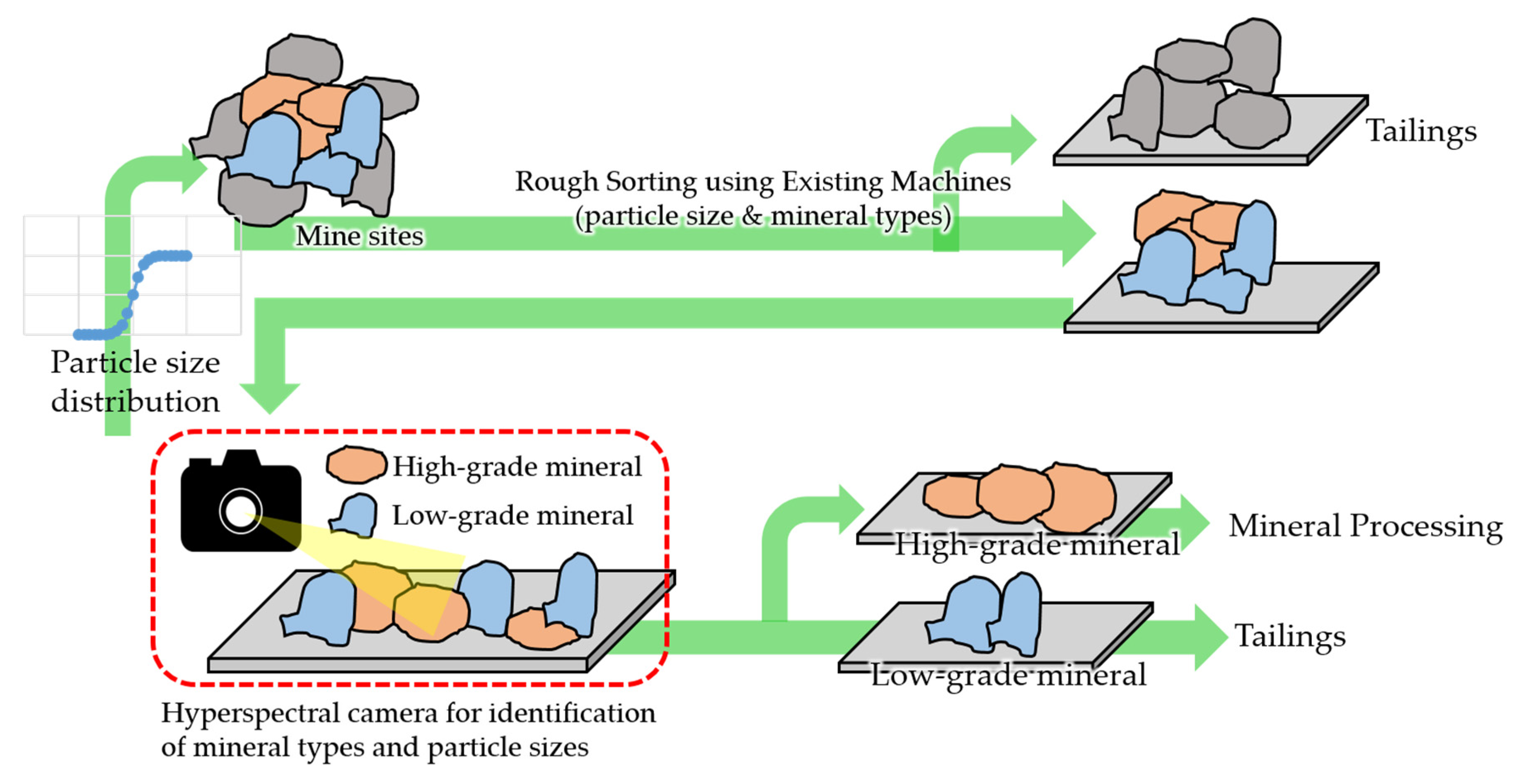
1.1. Background
1.2. Technics
2. Materials and Methods
2.1. Capturing RGB Images
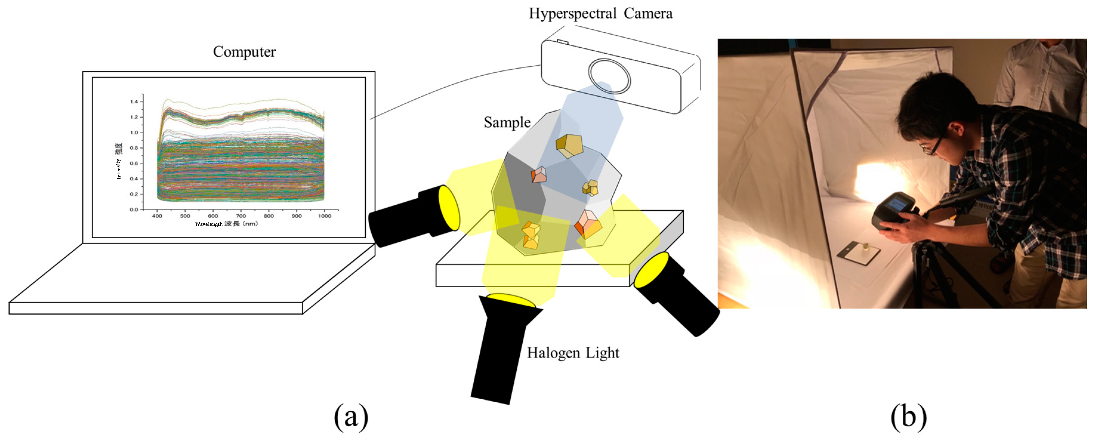
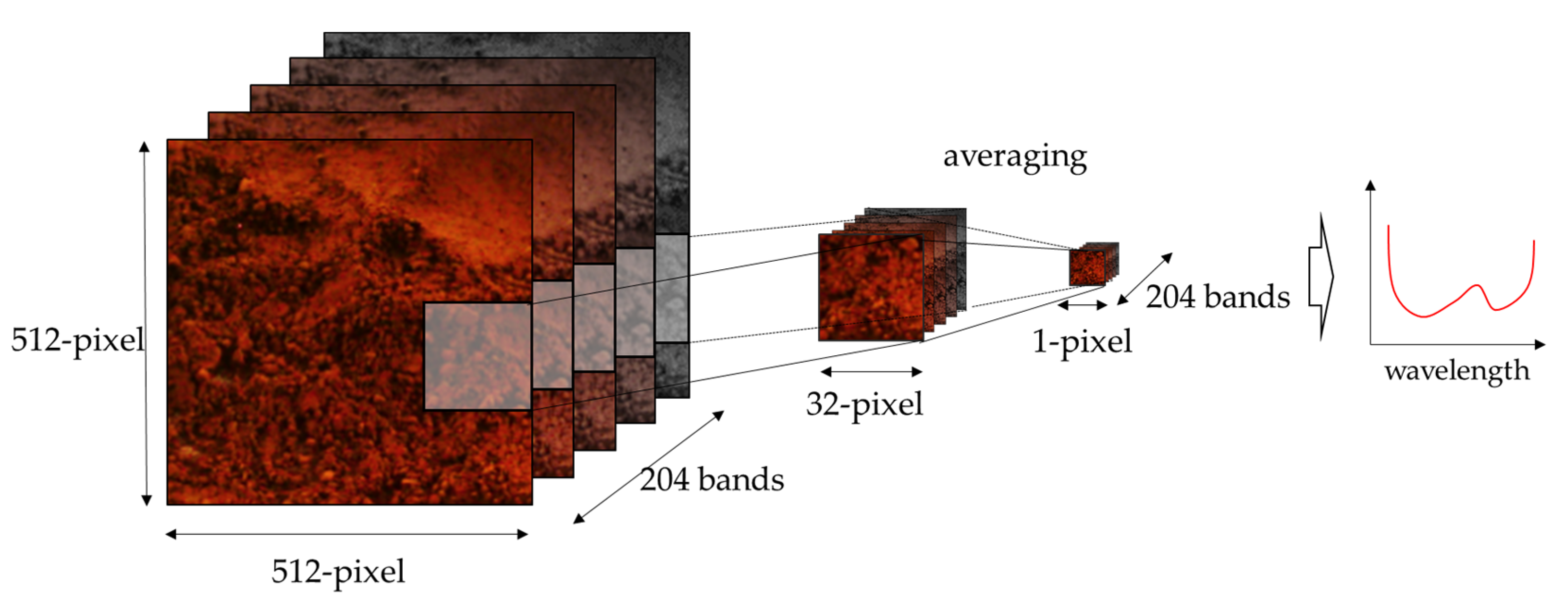
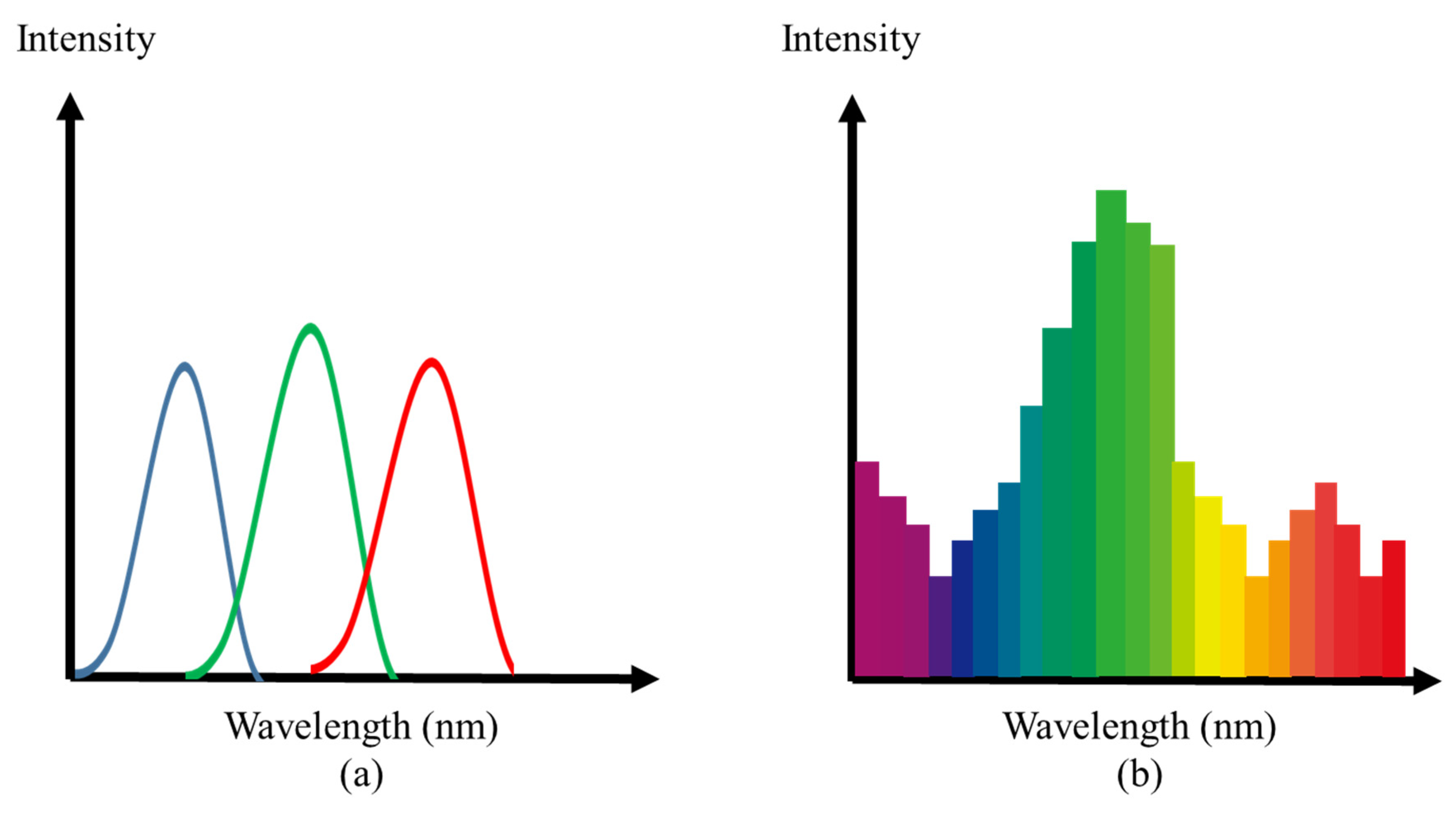
2.2. Capturing Hyperspectral Image
2.3. Experiment
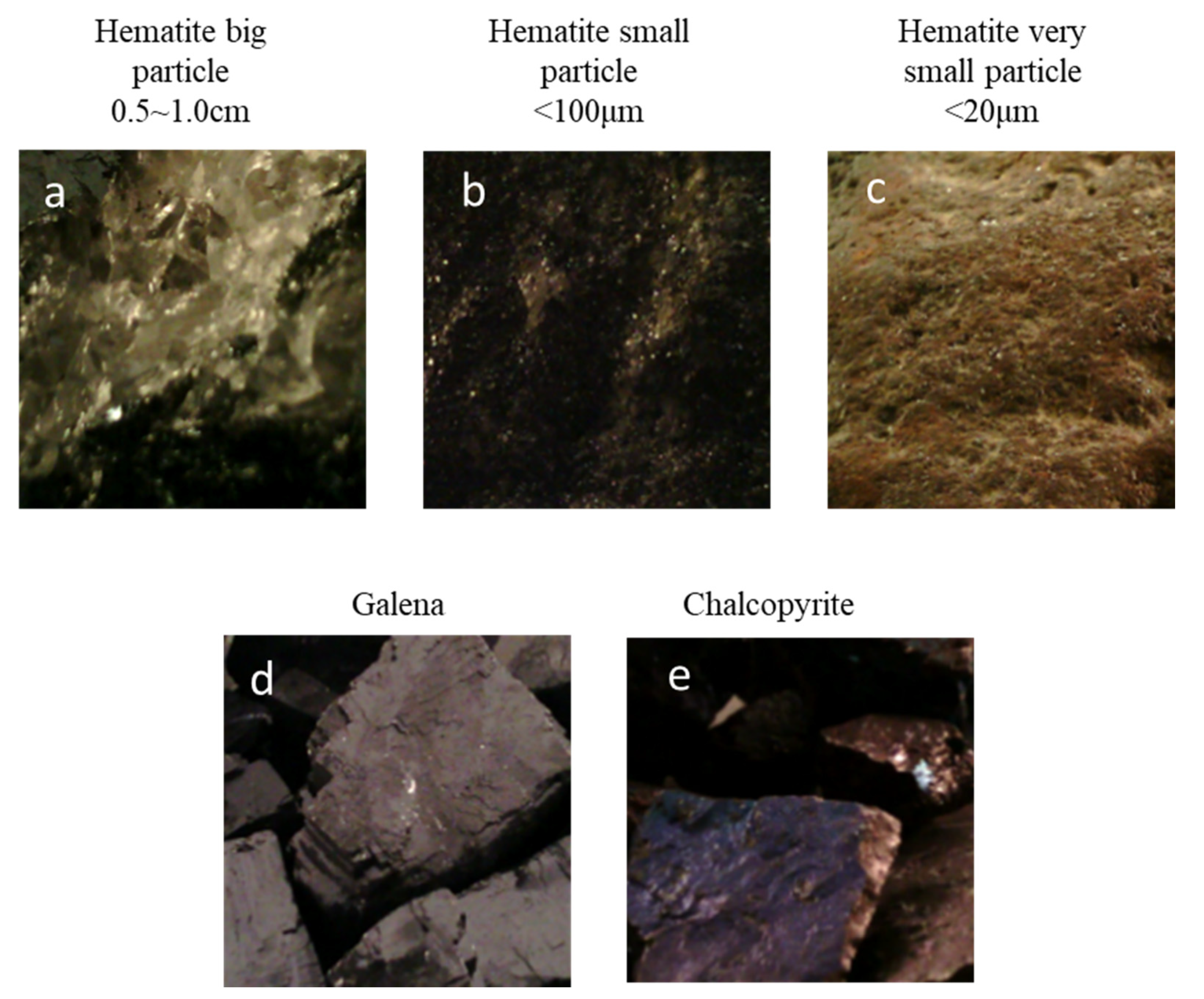
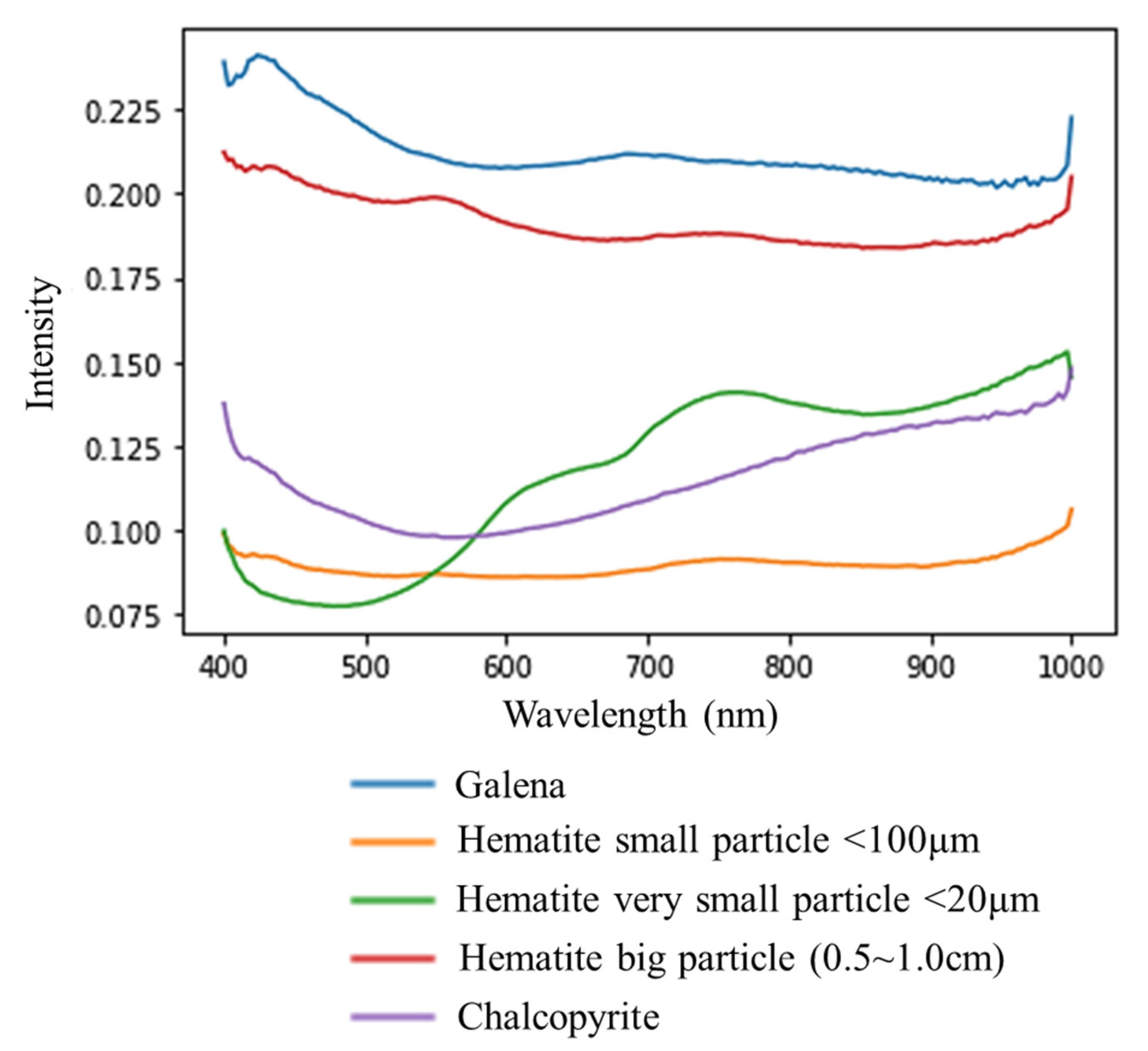
2.4. Obtained Images
3. Results
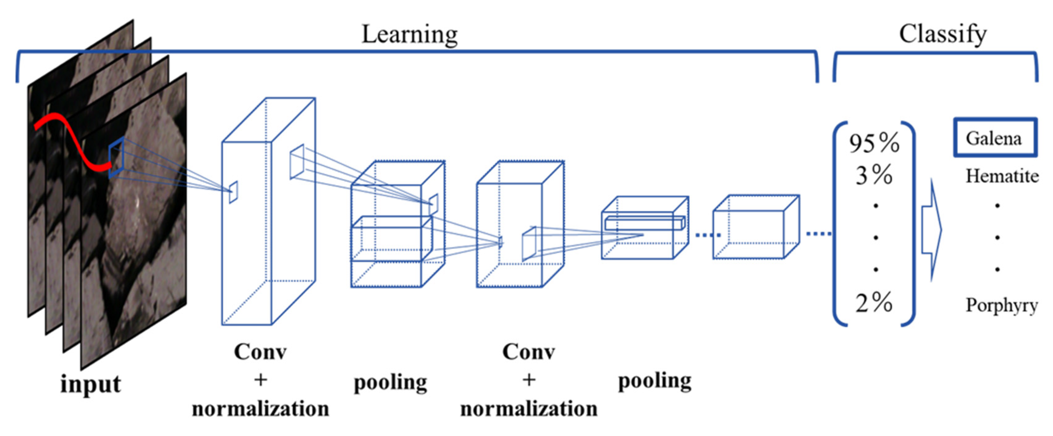
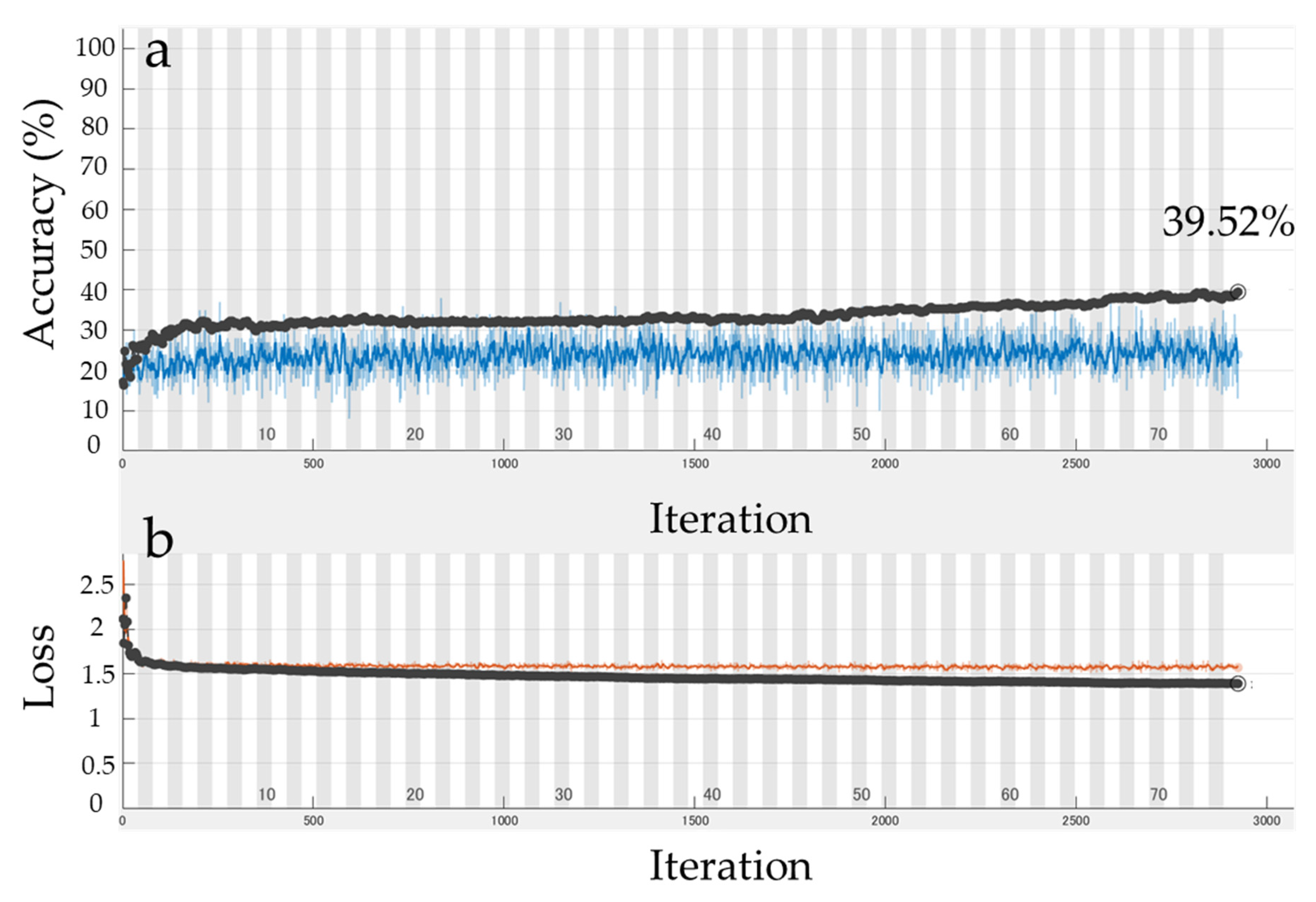
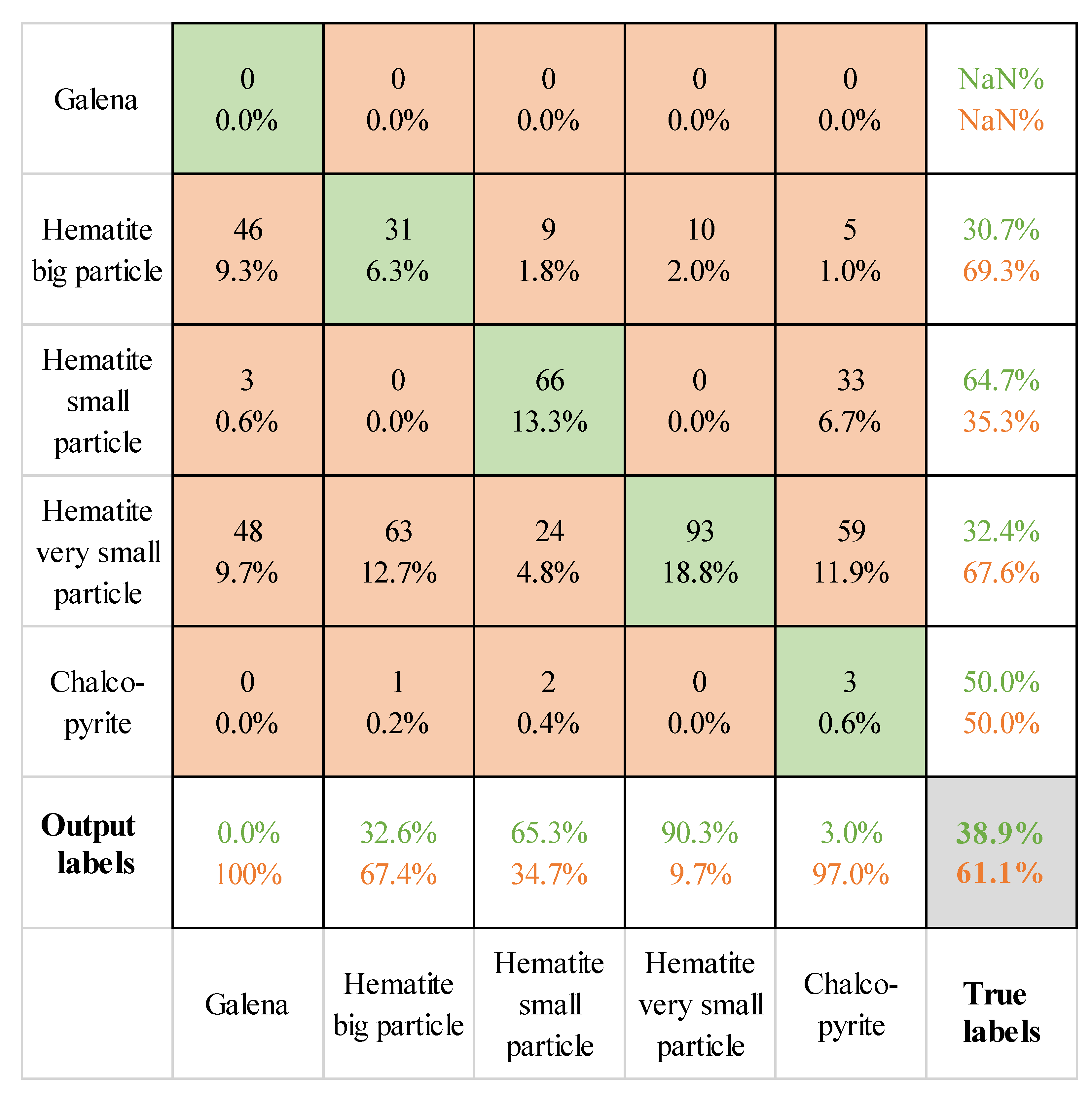
3.1. Deep Learning Analysis for RGB Images
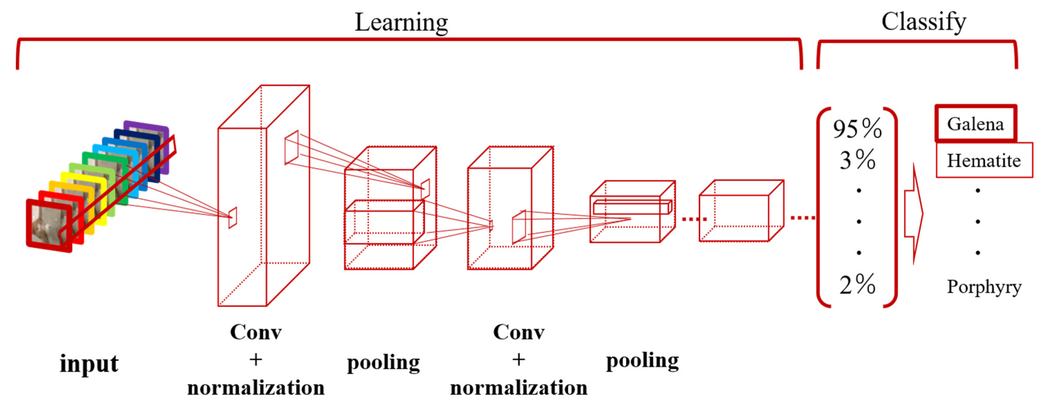
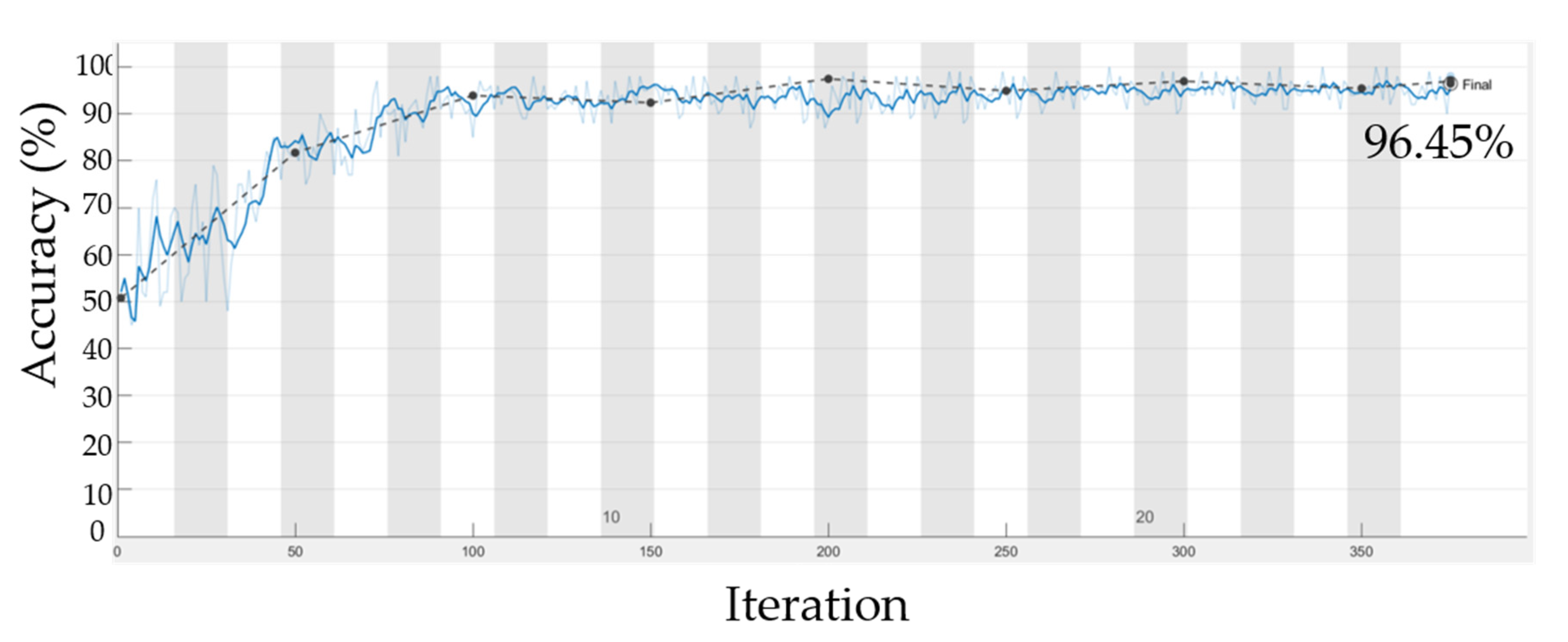
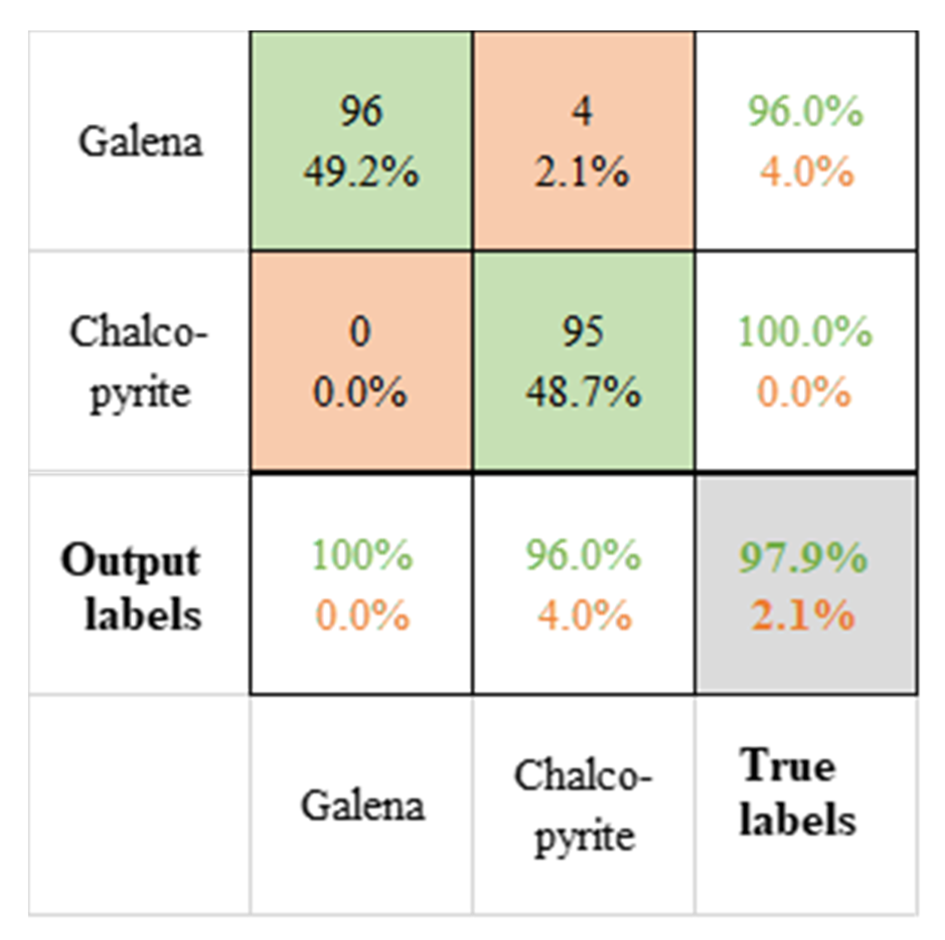
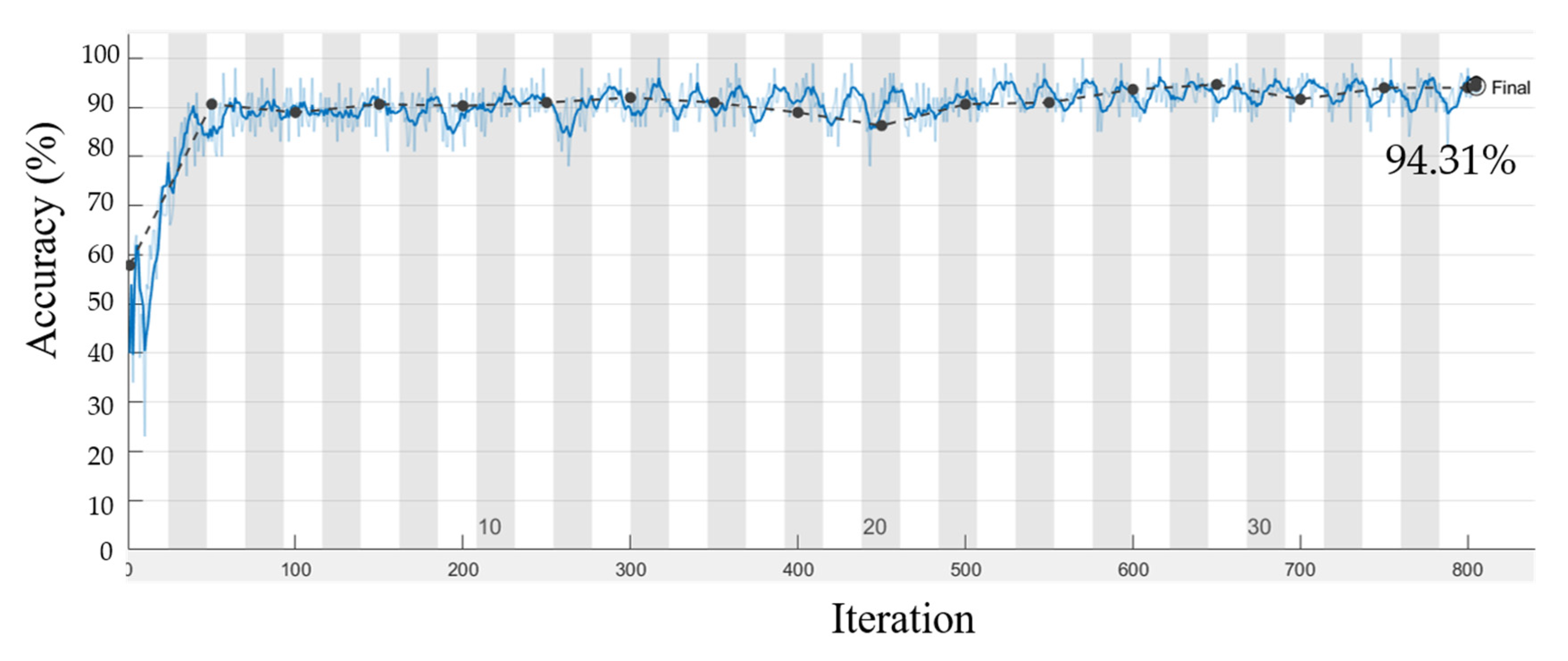
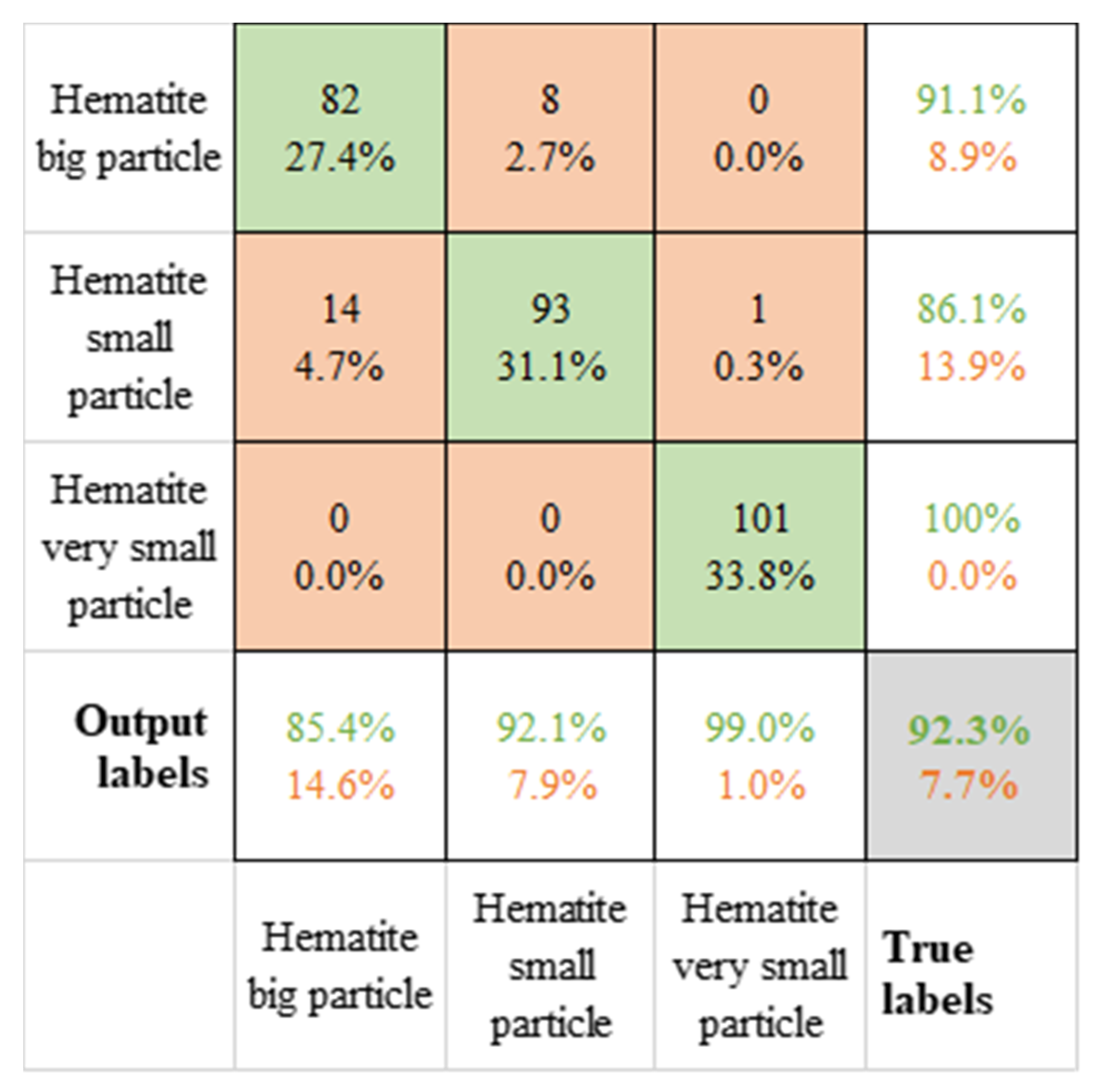
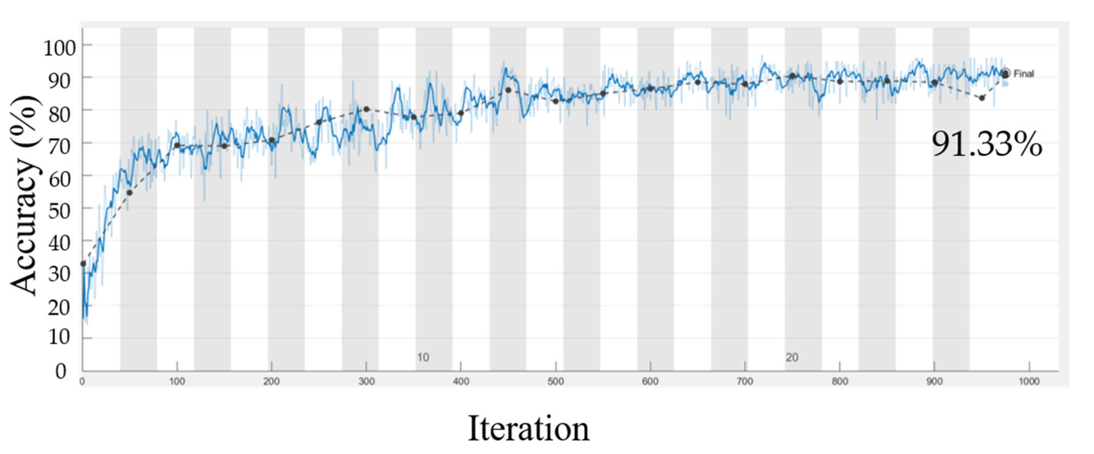
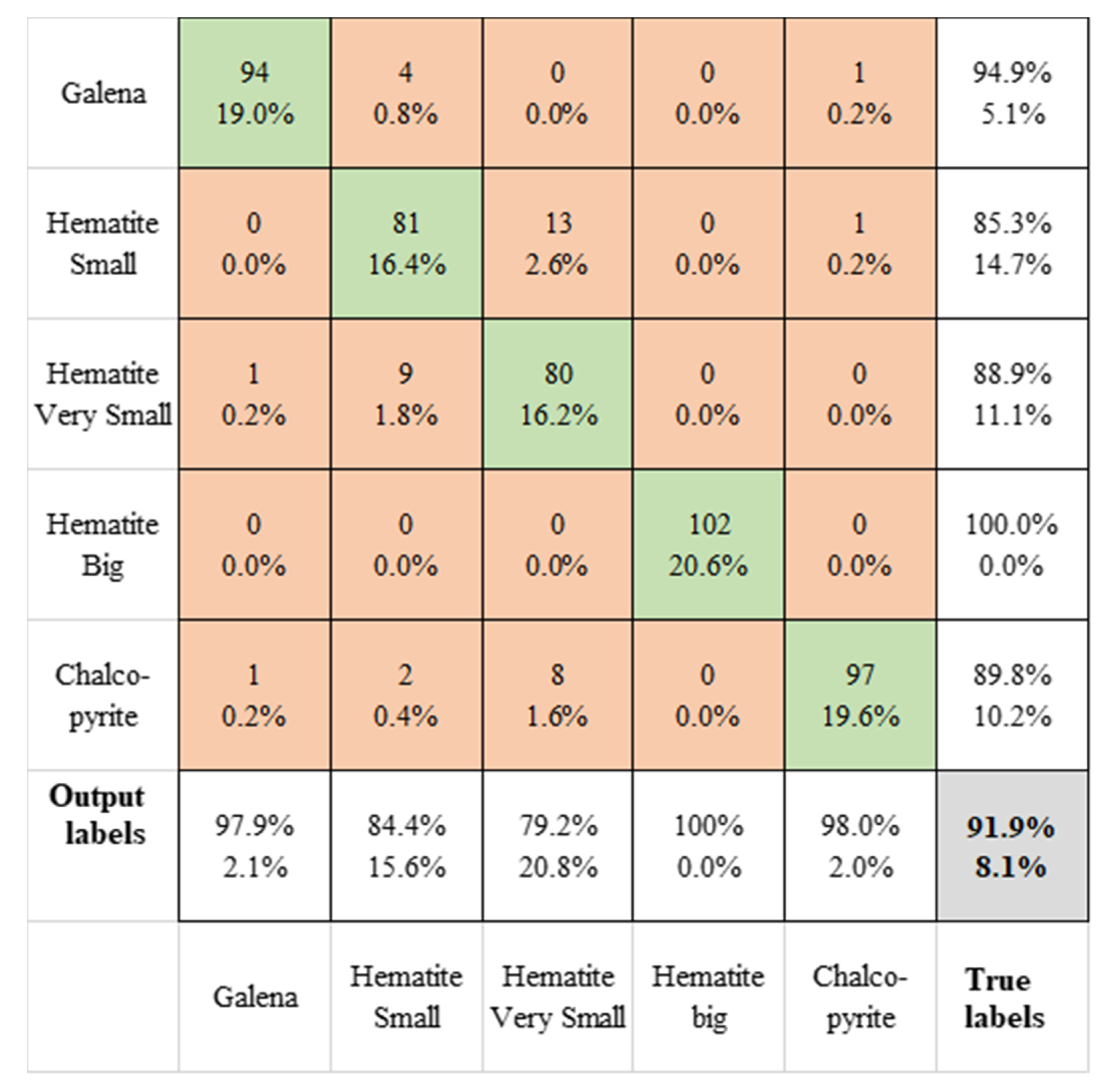
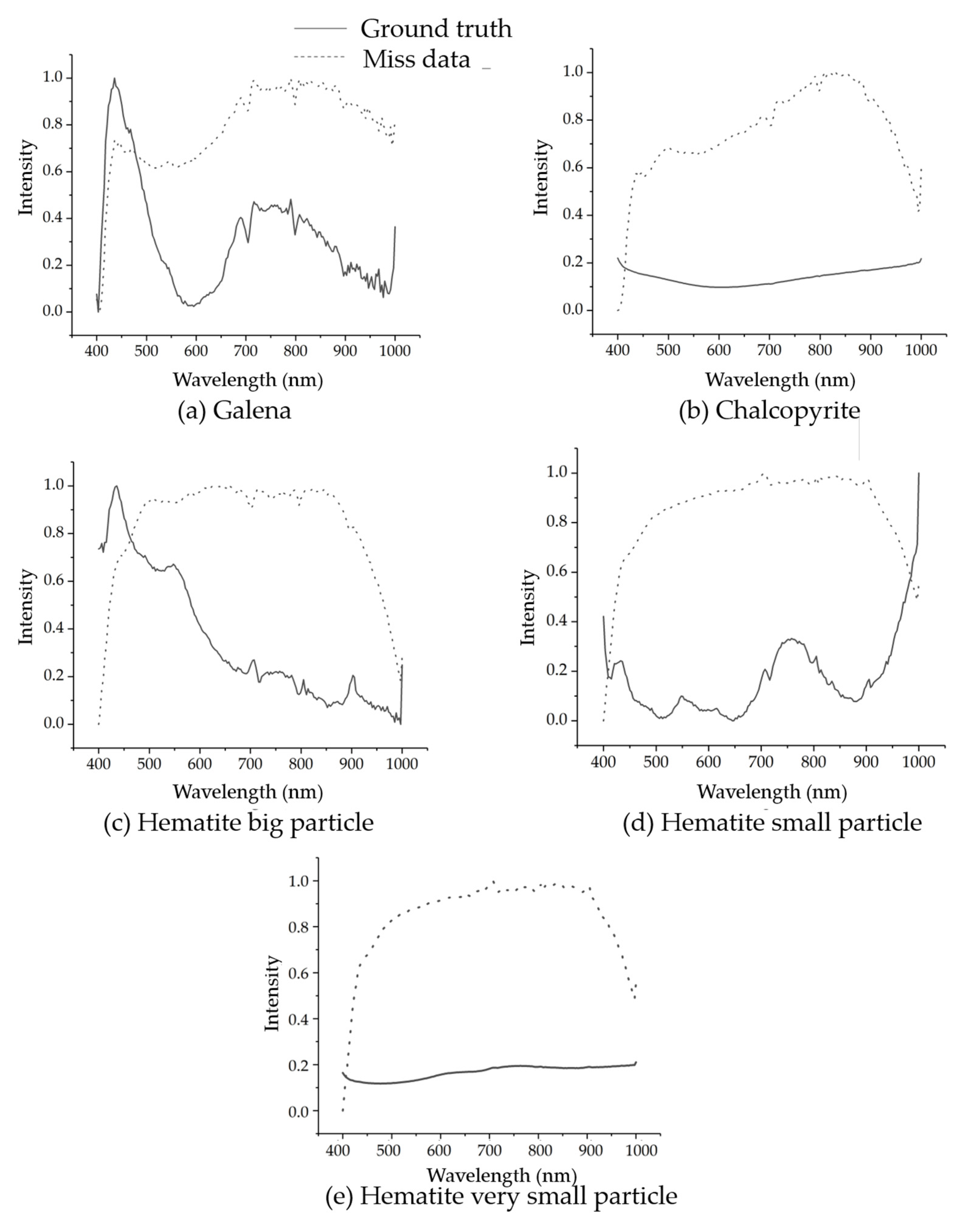
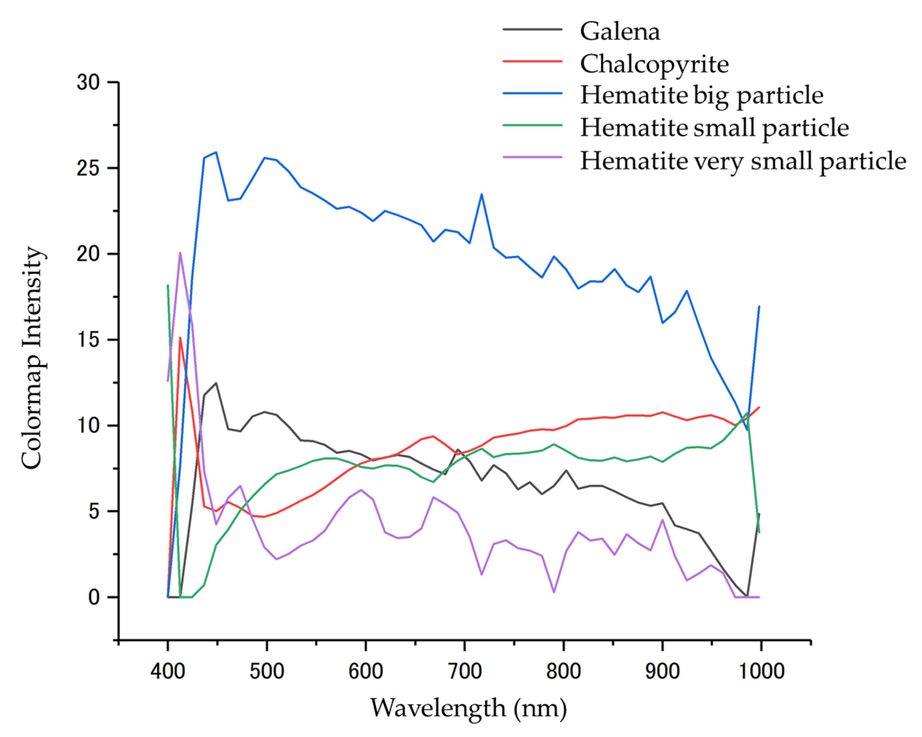
3.2. Deep Learning Analysis for Hyperspectral Data
4. Discussion
5. Conclusions
Author Contributions
Funding
Conflicts of Interest
References
- Perez, C.; Estévez, P.; Vera, P.; Castillo, L.; Aravena, C.; Schulz, D.; Medina, L. Ore grade estimation by feature selection and voting using boundary detection in digital image analysis. Int. J. Miner. Process. 2011, 101, 28–36. [Google Scholar] [CrossRef]
- Dumont, J.-A.; Lemos Gazire, M.; Robben, C. Sensor-based ore sorting methodology investigation applied to gold ores. In Procemin Geomet 2017; Gecamin: Santiago, Chile, 2017. [Google Scholar]
- Stone, A.M. Selection and sizing of ore sorting equipment. In Design and Installation of Concentration and Dewatering Circuits; Society of Mining Metallurgy and Exploration: New York, NY, USA, 1986. [Google Scholar]
- Han, B.; Altansukh, B.; Haga, K.; Stevanović, Z.; Jonović, R.; Avramović, L.; Urosević, D.; Takasaki, Y.; Masuda, N.; Ishiyama, D.; et al. Development of copper recovery process from flotation tailings by a combine method of high-pressure leaching-solvent extraction. J. Hazard. Mater. 2018, 352, 192–203. [Google Scholar] [CrossRef] [PubMed]
- Mokmeli, M. Pre feasibility study in hydrometallurgical treatment of low-grade chalcopyrite ores from Sarcheshmeh copper mine. Hydrometallurgy 2020, 191, 105215. [Google Scholar] [CrossRef]
- Schulz, B.; Merker, G.; Gutzmer, J. Automated SEM Mineral Liberation Analysis (MLA) with generically labelled EDX spectra in the Mineral processing of rare earth element ores. Minerals 2019, 9, 527. [Google Scholar] [CrossRef] [Green Version]
- Liu, C.; Li, M.; Zhang, Y.; Han, S.; Zhu, Y. An Enhanced rock mineral recognition method integrating a deep learning model and clustering algorithm. Minerals 2019, 9, 516. [Google Scholar] [CrossRef] [Green Version]
- Robben, C.; Wotruba, H. Sensor-based ore sorting technology in mining—Past, present and future. Minerals 2019, 9, 523. [Google Scholar] [CrossRef] [Green Version]
- Zhang, W.; Sun, W.; Hu, Y.; Cao, J.; Gao, Z. Selective flotation of pyrite from galena using chitosan with different molecular weights. Minerals 2019, 9, 549. [Google Scholar] [CrossRef] [Green Version]
- Sabins, F.F. Remote sensing for mineral exploration. Ore Geol. Rev. 1999, 14, 157–183. [Google Scholar] [CrossRef]
- Mezned, N.; Abdeljaoued, S.; Boussema, M.R. ASTER multispectral imagery for spectral unmixing based mine tailing cartography in the North of Tunesia. In Proceedings of the Remote Sensing and Photogrammetry Society Annual Conference, Newcastle upon Tyne, UK, 11–14 September 2007. [Google Scholar]
- Chabrillat, S.; Goetz, A.F.H.; Olsen, H.W. Field and Imaging spectrometry for indentification and mapping of expansive soils. In Imaging Spectrometry; Springer: Dordrecht, The Netherlands, 2002. [Google Scholar]
- Dominy, S.C.; O’Connor, L.; Parbhakar-Fox, A.; Glass, H.J.; Purevgerel, S. Geometallurgy—A Route to More Resilient Mine Operations. Minerals 2018, 8, 560. [Google Scholar] [CrossRef] [Green Version]
- Brough, C.P.; Warrender, R.; Bowell, R.J.; Barnes, A.; Parbhakar-Fox, A. The process mineralogy of mine wastes. Miner. Eng. 2013, 52, 125–135. [Google Scholar] [CrossRef]
- Pierre-Henri, K.; Jan, R. Sequential decision-making in mining and processing based on geometallurgical inputs. Miner. Eng. 2020, 149, 106262. [Google Scholar]
- Farooq, S.; Govil, H. Mapping regolith and gossan for mineral exploration in the Eastern Kumaon Himalaya, India using hyperion data and object oriented image classification. Adv. Space Res. 2014, 53, 1676–1685. [Google Scholar] [CrossRef]
- Sinaice, B.; Youhei, K.; Takeshi, S.; Jo, S.; Hibiki, Y.; Yutaka, I.; Shinji, U. Development of a differentiation and identification system for igneous rocks using hyper-spectral images and a convolutional neural network (CNN) system. In Proceedings of the MMIJ 2017, Sapporo, Japan, 26–28 September 2017. [Google Scholar]
- Zhang, L.; He, Z.; Liu, Y. Deep object recognition across domains based on adaptive extreme learning machine. Neurocomputing 2017, 239, 194–203. [Google Scholar] [CrossRef]
- Sathya, R.; Annamma, A. Comparison of supervised and unsupervised learning algorithms for pattern classification. IJARAI 2013, 2, 34–38. [Google Scholar] [CrossRef] [Green Version]
- Zhong, Z.; Jin, L.; Xie, Z. High performance offline handwritten Chinese character recognition using GoogLeNet and directional feature maps. ICDAR Tunis. 2015, pp. 846–850. Available online: https://arxiv.org/ftp/arxiv/papers/1505/1505.04925.pdf (accessed on 13 September 2020).
- Jo, S.; Youhei, K.; Syun, M.; Takeshi, S. Early diagnosis of rotary percussion drill bits using machine learning -In case of time-frequency contents as an input. In Proceedings of the MMIJ 2018, Fukuoka, Japan, 24–26 September 2018. [Google Scholar]
- Chen, X.; Guo, J.; Li, H. Implementation and practice of an integrated process to recover copper from low gade ore at Zijinshan mine. Hydrometallurgy 2020, 195, 105394. [Google Scholar] [CrossRef]
- Padilla, R.; Jerez, O.; Ruiz, M.C. Kinetic of the pressure leaching of enargite in FeSO4-H2SO4-O2 media. Hydrometallurgy 2015, 158, 49–55. [Google Scholar] [CrossRef]
- Szegedy, C.; Liu, W.; Jia, Y.; Sermanet, P.; Reed, S.; Anguelov, D.; Erhan, D.; Vanhoucke, V.; Rabinovich, A. Going deeper with convolutions. Cornell Univ. 2014, 1409, 1–9. [Google Scholar]
- Simonyan, K.; Zisserman, A. Very deep convolutional networks for large-scale image recognition. ICLR 2015 2015, 1409, 1556. [Google Scholar]


| Layers | Layer Size | Stride | Padding Size | Layers | Layer Size | Stride | Padding Size |
|---|---|---|---|---|---|---|---|
| ImageInputLayer | [1, 204] | - | - | Convolution2dLayer | [1, 3] | 1 | [0, 1] |
| Convolution2dLayer | [1, 3] | 1 | [0, 1] | Convolution2dLayer | [1, 3] | 1 | [0, 1] |
| Convolution2dLayer | [1, 3] | 1 | [0, 1] | BatchNormalizationLayer | - | - | - |
| BatchNormalizationLayer | - | - | - | ReluLayer | - | - | - |
| ReluLayer | - | - | - | MaxPooling2dLayer | [1, 2] | [1, 2] | - |
| MaxPooling2dLayer | [1, 2] | [0, 1] | FullyConnectedLayer | - | - | - | |
| Convolution2dLayer | [1, 3] | 1 | [0, 1] | FullyConnectedLayer | - | - | - |
| Convolution2dLayer | [1, 3] | 1 | [0, 1] | FullyConnectedLayer | - | - | - |
| BatchNormalizationLayer | - | - | - | SoftmaxLayer | - | - | - |
| ReluLayer | - | - | - | ClassificationLayer | - | - | - |
| MaxPooling2dLayer | [1, 2] | [1, 2] | - |
| RGB Images 16 × 16 × 3 Pixels | Training Data | Validation Data | Test Data | Total |
|---|---|---|---|---|
| Galena | 770 | 96 | 97 | 963 |
| Chalcopyrite | 770 | 97 | 97 | 994 |
| Hematite large particles | 765 | 95 | 96 | 956 |
| Hematite small particles | 806 | 101 | 101 | 1008 |
| Hematite very small particles | 819 | 103 | 102 | 1024 |
| Five Types of Minerals | |
|---|---|
| Final accuracy | 39.52% |
| Hyperspectral Data 1 × 1 × 204 Pixels | Training Data | Validation Data | Test Data | Total |
|---|---|---|---|---|
| Galena | 770 | 96 | 97 | 963 |
| Chalcopyrite | 770 | 97 | 97 | 994 |
| Hematite large particles | 765 | 95 | 96 | 956 |
| Hematite small particles | 806 | 101 | 101 | 1008 |
| Hematite very small particles | 819 | 103 | 102 | 1024 |
| Hyperspectral Data | RGB Images | |||
|---|---|---|---|---|
| Learning Options | Two Types of Minerals | Three Different Grain Sizes of Hematite | Five Types of Minerals | Five Types of Minerals |
| Optimizer | ADAM | ADAM | ADAM | SGDM |
| Mini Batch Size | 100 | 100 | 100 | 100 |
| Max Epochs | 25 | 50 | 100 | 75 |
| Elapsed time | 15 min | 61 min | 253 min | 94 min |
| Initial Learn Rate | 1.00E-04 | 1.00E-04 | 1.00E-04 | 1.00E-04 |
© 2020 by the authors. Licensee MDPI, Basel, Switzerland. This article is an open access article distributed under the terms and conditions of the Creative Commons Attribution (CC BY) license (http://creativecommons.org/licenses/by/4.0/).
Share and Cite
Okada, N.; Maekawa, Y.; Owada, N.; Haga, K.; Shibayama, A.; Kawamura, Y. Automated Identification of Mineral Types and Grain Size Using Hyperspectral Imaging and Deep Learning for Mineral Processing. Minerals 2020, 10, 809. https://doi.org/10.3390/min10090809
Okada N, Maekawa Y, Owada N, Haga K, Shibayama A, Kawamura Y. Automated Identification of Mineral Types and Grain Size Using Hyperspectral Imaging and Deep Learning for Mineral Processing. Minerals. 2020; 10(9):809. https://doi.org/10.3390/min10090809
Chicago/Turabian StyleOkada, Natsuo, Yohei Maekawa, Narihiro Owada, Kazutoshi Haga, Atsushi Shibayama, and Youhei Kawamura. 2020. "Automated Identification of Mineral Types and Grain Size Using Hyperspectral Imaging and Deep Learning for Mineral Processing" Minerals 10, no. 9: 809. https://doi.org/10.3390/min10090809