Article

3D Spatial Distribution of Arsenic in an Abandoned Mining Area: A Combined Geophysical and Geochemical Approach

by
Jesús Ruiz-Roso
1,
Mari Luz García-Lorenzo
1,*,
Pedro Castiñeiras
1,
Alfonso Muñoz-Martín
2 and
Elena Crespo-Feo
1
1
Facultad de Ciencias Geológicas, “Geochemistry: Exploration and Environment” UCM Research Group. Departamento de Mineralogía y Petrología, Universidad Complutense de Madrid, 28040 Madrid, Spain
2
Facultad de Ciencias Geológicas, “Tectonofísica Aplicada” UCM Research Group. Departamento de Geodinámica, Estratigrafía y Paleontología, Universidad Complutense de Madrid, 28040 Madrid, Spain
*
Author to whom correspondence should be addressed.
Minerals 2020, 10(12), 1130; https://doi.org/10.3390/min10121130
Submission received: 3 November 2020 / Revised: 1 December 2020 / Accepted: 8 December 2020 / Published: 15 December 2020
(This article belongs to the Special Issue Environmental Geochemistry of Mineral Deposits)

Abstract

:
Abandoned mine wastes, containing high sulfide contents, are of particular concern because of the formation of acid mine drainage (AMD), becoming an active and harmful point source of potentially toxic elements (PTEs) to the environment. A detailed evaluation of the chemical and mineralogical composition of mining wastes is necessary to determine effective remediation actions. Due to the high amount of generated wastes as a result of mining and processing activities, the cost and time consumed for this characterization are limiting. Hence, efficient tools could be applied to predict the composition of these wastes and their spatial distribution. This study aims to determine the physico-chemical characterization of wastes from mining activities using geochemical and geophysical techniques. The obtained results, both geochemical and geophysical, allow us to locate areas with a high potential risk of contamination by As in an economic and simple way, and enable us to design detailed geochemical sampling campaigns. In addition, the fact that there are conductive fractures in depth suggests the possible circulation of contaminants through them as well as the preferential lines of circulation.

1. Introduction

Arsenic is a natural component of the Earth’s crust. The arsenic concentrations in natural soils are low, the mean concentration in igneous rocks ranges from 1.5 to 3.0 mg kg−1, whereas in sedimentary rocks, it ranges from 1.7 to 400 mg kg−1 [1,2].
More than 300 As-bearing minerals are found in nature, the most abundant being arsenopyrite (FeAsS), commonly found in pegmatites, high-temperature gold-quartz, and tin veins, and also in contact with metamorphic sulfide deposits [1,3].
However, on certain occasions, the natural contents are increased due to various industrial activities, causing soil contamination. Among them, metal mining extraction is one of the sectors that produce this type of effects to a greater extent, by favoring the dispersion of potentially toxic elements (PTEs) contained in mining materials, both before the exploitation (geochemical anomalies) and after, by allowing the dispersion of PTEs.
Currently, mines are typically designed to mitigate their potential environmental impacts, but the extracted mineral deposits of old mines often remain where they were dumped outside after mining activity was stopped [4]. Mine wastes containing high sulfide concentrations are one of the most serious sources of environmental pollution of metal (oids) and other potentially toxic elements, which is due to the potential production of acid drainage of mine drainage (AMD) formed by the oxidation of sulfide mineral, commonly pyrite [5].
The principal source of arsenic is arsenical pyrite that undergoes oxidation releasing As(III) and As(V) to aquatic systems, according to simplified reactions [6]:
FeS2-x Asx (arsenical pyrite) + 3.5 O2 + H2O→Fe2+(aq) + 2SO42− + 2H+ + As5+/As3+
FeS2−xAsx (arsenical pyrite) + 14Fe3+(aq)+8H2O→15Fe2+(aq)+2SO42−(aq)+16H++As5+/As3+(aq)
AMD is produced when sulfide-bearing material comes into contact with oxygen and water Equation (1). As a result of this oxidation reaction, the pH decreases giving rise to the reaction Equation (2), where Fe3+ comes from the oxidation of ferrous iron (Fe2+) and partial dissolution of hematite/goethite.
As species are influenced by different geochemical factors, such as pH-Eh conditions, temperature, sulfate concentrations, and bacterial activity. Depending on these conditions, arsenic ions can remain in solution or undergo multiple sorption/desorption cycles during the formation of acid mine precipitates. Arsenic exists in the −3, 0, +3, and +5 oxidation states; however, arsenite (As (III) and arsenate (As (V)) are the most frequently found in waters [7,8].
An analysis of a site affected by PTEs requires a great deal of time, as well as the application of various analytical techniques, such as acid digestion, chemical simple extraction, mineralogical and textural composition. To add to that, to perform this characterization, it is necessary to collect and transport the samples to the place of analysis, making the procedure more expensive.
Cost-saving and faster alternatives useful for screening could be used as a complement of traditional laboratory analysis [9]. Among them, geophysical techniques are being applied in environmental studies to characterize contaminated sites, counting among their advantages that they are non-invasive techniques and that they allow one to obtain a high density of information at a low cost [10,11].
The objective of this study is to analyze the potential of electromagnetic techniques when examining the contamination of an old mining area in Guadalix de la Sierra (Madrid, Spain) potentially contaminated by arsenic. For this aim, an electromagnetic system in the frequency domain (FDEM) has been used and allows investigating the resistivity and phase component of soils until 3.3 m deep. Resistivity tomographic image reconstruction of soils has been made, and the obtained results have been compared with those obtained in the geochemical characterization, to determine the relationship between the geochemical and geophysical parameters. The results can help to locate areas of potential pollution, not detected in the geochemical analysis due to their lower spatial resolution, and to design new geochemical characterization campaigns.

2. Geological Setting

The Spanish Central System is part of the northern domain of the Central Iberian Zone of the Iberian Massif [12], and it has been classically divided into three sectors (Figure 1), from W to E: Gredos, Guadarrama, and Somosierra-Ayllón [13]. The study area is located in the SE limit between the Guadarrama and the Somosierra-Ayllón sectors. The Guadarrama sector is characterized by the presence of an alleged pre-Ordovician metasedimentary series composed of paragneiss, calc-silicate rocks, paramphibolite, and marble; Ordovician felsic igneous rocks metamorphosed into Augen gneisses during the Variscan orogen are also present, and late Variscan granitoids are abundant, especially to the West. Metamorphism varies between intermediate grade (Sil zone), nearby the limit with the Somosierra-Ayllón sector, and high grade (Sil+Kfs zone) to the West, with large areas close to anatexis.
The study area is mainly constituted by Augen gneisses (Figure 1) that are crosscut by dykes of varied composition: microdiorite, quartz, and felsic pegmatite. The mineralization is linked to the latter, which are 1–2 m thick and tens of meters long. Their orientation is roughly NE–SW, subvertical, and they are probably related to a late Variscan fracturing. The felsic pegmatite dykes are composed of quartz, K-feldspar (orthose), plagioclase, and abundant muscovite. The genesis of the Sn-W deposit has been interpreted as hydrothermal of high-temperature [16].
The quaternary cover is of minor importance and it consists of anthropic material from the mining activities and river deposits. The mining activities in the area began in the fifteenth century, as a silver ore, but the peak of activity took place in the middle eighteenth century and during the Second World War. They obtained first As from arsenopyrite (FeAsS), and then W from Mn-rich wolframite (hubnerite, MnWO4). Arsenopyrite is frequently altered to scorodite (FeAsO4·2H2O) and associated with columbite-(Fe) (FeNb2O6), sphalerite ((Zn,Fe)S), galena (PbS), matildite (AgBiS) and accessory uraninite (UO2) [16].
The experiment was conducted in abandoned mine exploitation located in the upper portion of a small sub-catchment of the Guadalix River (Madrid, Spain), which feeds into the Madrid Tertiary Detrital Aquifer, which supplies water to the population of Madrid. The site includes an abandoned smelting factory where arsenopyrite was processed for the extraction of wolfram during the Second World War. The mining wastes, which contain up to 19 g kg−1 of As and currently remain where they were dumped on the soil surface, are subject to weathering processes [4,17].

3. Materials and Methods

3.1. Geochemical Characterization: Data and Methods

Soil sampling has been designed to analyze the concentration and mobility of arsenic, and a systematic sampling (grid) was proposed, with 27 sampling points (Figure 2a,b).
Sampling was performed according to ISO 10381-1:2002 [18]. In each monitoring plot, five subsamples were collected from the top layer (0–20 cm) at the center and on the diagonal lines of the plot (1 × 1 m). Samples were collected with a shovel in each subplot, then mixed and homogenized and a subsample (about 2 kg) was taken.

3.1.1. Chemical Analysis

All samples were air-dried and sieved through a 2 mm screen. The pH and electrical conductivity (EC) were determined in a 1:5 (w/v) suspension of soil in pure, deionized water (Milli-Q; resistivity ≥ 18 MO hm).
Total PTEs content: The soils were first ground to a fine powder using a zirconium ball mill. Aliquots (0.1 g) of soil samples were placed in Teflon vessels, and a mixture of 5 ml concentrated HF (37%), 200 μL concentrated HNO3 (65%) and 5 mL of water was added. After digestion in a conventional microwave oven, the solutions were transferred to a volumetric flask, brought to 50 mL, and analyzed.
All collected samples were submitted to an acid extraction, simulating the effect of acid mine drainage in selected materials following the ISO 17586:2016 procedure [19].
The arsenic content was measured by atomic fluorescence spectrometry using an automated continuous flow hydride generation spectrometer (PSA Millenium Merlin 10055). The limit of quantification for the selected elements was 0.3 μg kg−1 for arsenic.
Accuracy and precision of the analytical procedures for As concentration was verified using the certified reference material SRM 2710 Montana Soil. The results were consistent with the certified values with errors of < 5%. Element concentration in procedure blanks and all reagents were always below the detection limit.
The analytical determinations were carried out in the University Complutense of Madrid (Spain) and the University of Castilla La Mancha (Spain).

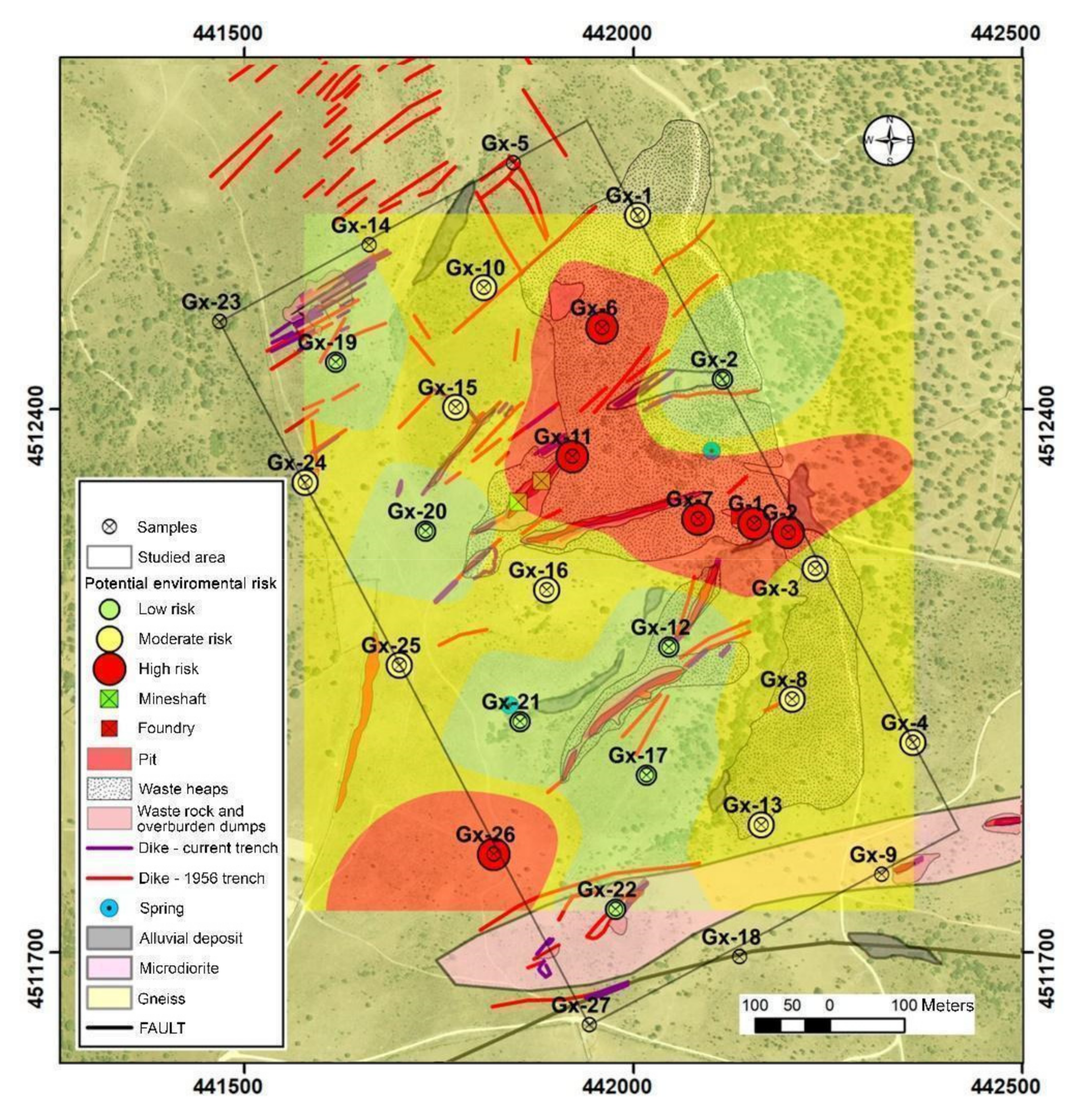
3.1.2. Assessment of Potential Environmental Risk

A significant number of indicators designed to approximate the quality of soils can be found in the literature. In our case, the assessment of sediment contamination level was performed by the quantification of the contamination factor (CF) and the acid mine drainage mobility indicator [20,21,22,23].
The contamination factor (CF) has been calculated as the ratio between the metal concentrations with its background values:
C F = C s o i l C b a c k g r o u n d
The criteria adopted to determine the extent of the contamination were as follows: no/low contamination (CF < 1), moderate (1 ≤ CF < 3), high (3 ≤ CF < 6), and very high (CF ≥ 6). The value 5.8 mg kg-1 was taken as a background element based on the reference [24].
In addition to the contamination factor, acid mine drainage mobility indicator was calculated to provide information of As mobilization in materials with a high probability of being affected by AMD. This indicator is calculated as the quotient between the arsenic concentration with its background values after the nitric extraction:
A M I n n = C s a m p l e   a f t e r   a c i d   e x t r a c t i o n C b a c k g r o u n d   a f t e r   a c i d   e x t r a c t i o n
Indicator values lower than 1 point to low mobility; values from 1 to 3 suggest moderate mobility; from 3 to 6, considerable mobility and higher than 6 very high mobility.

3.1.3. Geochemical Data Processing

To geologically and spatially contextualize the distribution of arsenic, geological maps were carried out together with environmental liabilities of mining using “Autocad 2011 (Autodesk)” and the ArcGIS software geographic information system.
To carry out the fieldwork with a sufficient degree of detail, it has been necessary to develop an ad hoc detailed mapping, taking into account that the best available scale is 1:25000, which was insufficient to map elements such veins or dumps, as their dimensions are less than 3–4 m. Thus, using the ArcGIS geographic information system and based on the PNOA digital terrain model (MDT05-LIDAR), two topographic plans with equidistant contour lines 30 and 50 cm were elaborated with which it was possible to visualize all the terrain features susceptible to map. A slope map was also prepared.
Spatial interpolation and geographical information system mapping techniques were employed to produce spatial distribution maps for the target elements. For this purpose, ArcGIS v.10.4 software (Esri, Redlands, CA, USA) was used. The sampling points, defined by a global positioning system (GPS), were integrated to create a database in which the coordinates and the value of the element concentrations for each point were included. For the spatial distribution of the As and Sb contents, five intervals were considered: (minimum–p25), (p25–p50), (p50–p75), (p75–p95) and (p95–maximum).

3.2. Geophysical Data and Methods

Once the geochemical characterization had been carried out, a field campaign was conducted to characterize the distribution of resistivities in the study area. Given the large surface to be investigated, the orography and the necessary penetration (< 4 m), the inductive EM system CMD-Explorer (GF Instruments) was selected. The equipment is a conductivity ground meter (CGM) consisting of three pairs of receiving (Rx) and transmitting (Tx) antennas mounted on a bar, which allows parameters to be obtained at three depths simultaneously. In this way, for each measurement point, the equipment obtains three values of apparent resistivity (ρap, Ω·m) and three values of in-phase component (in ppm) simultaneously at three depths. The value of the resistivity of rocks and soils (Ω · m) depends on their composition and the quantity and nature of the fluids they contain. Clay minerals have low resistivity (< 10 Ω·m), and resistivity decreases with alteration (weathering) of rocks and with the presence of fluids. Thus, resistivity is a parameter that allows distinguishing well between soils and surface, or remobilized deposits, from the fresh rock. Within the fresh rock, the resistivity allows identifying the hydraulically conductive zones, which, in this geological context, are fundamentally fractures [25,26].
The in-phase component is defined as the relative amount (in ppm) of the primary magnetic field and is directly related to the magnetic susceptibility of the measured material. This factor is especially useful for locating artificial metal objects such as cables or pipes. In this work, this parameter has been used as a quality criterion for the apparent resistivity values, using the resistivity values in the interpretation when the in-phase component values were stable.
The depth of penetration in conductivity meters (CGM) depends on the separation and orientation of coils and the operating frequency. In this case, the objective was to characterize potentially contaminated soils, which are poorly developed. For this reason, the “low” mode has been selected, which provides apparent resistivity values at 1.1 m, 2.2 m, and 3.3 m deep. In the NE sector of the study area, the “high” mode has also been used, which provides apparent resistivity values at depths of 2.2 m, 4.4 m, and 6.6 m, because in that area the soil thickness was potentially greater.
The acquisition was carried out in continuous mode with GPS positioning, with a measurement value every second, which allowed obtaining a high number of data in one day of exploration. The sampling trajectory was carried out through a zigzag route with NW-SE and NE-SW path lines (Figure 2b). In total, 32964 measurements were collected in “low” mode distributed in 5494 points in the study area (Figure 2b): 3 apparent resistivity data and 3 in-phase component data at each point, and 10122 measurements along 1687 measurement points in “high” mode. All this information has been referenced with UTM zone 30N (WGS84) coordinates and the IGN DEM elevation of 5 m horizontal resolution has been assigned to them. This large amount of information has been processed with the Oasis Montaj software.

3.2.1. Geophysical Data Processing

After data acquisition, quality control of the data (QC analysis) was performed, discarding less than 1% of them due to high errors (RMS> 10%), and unstable in-phase component values. Maps of apparent resistivity and maps of the in-phase component of the study area were made at the three depths measured with the LOW mode. To do so, the data have been filtered and interpolated using kriging with a linear variogram and a mesh pitch of 5 m.

3.2.2. Resistivity tomographic inversion

To obtain the resistivity structure in-depth, 7 longitudinal profiles have been sampled with regularized values every 5 m (Figure 2b). These data have been converted into the files necessary to carry out the tomographic inversion with the RES2DINV software [27,28,29]. The inversion of apparent resistivity values has been made using rectangular finite elements, and four nodes per element. The result of the inversion provides the real resistivity values of the subsoil at depth along the sections. In this way, the real resistivity values can be interpreted in terms of mineralogical composition, water content, degree of weathering, etc.

4. Results and Discussion

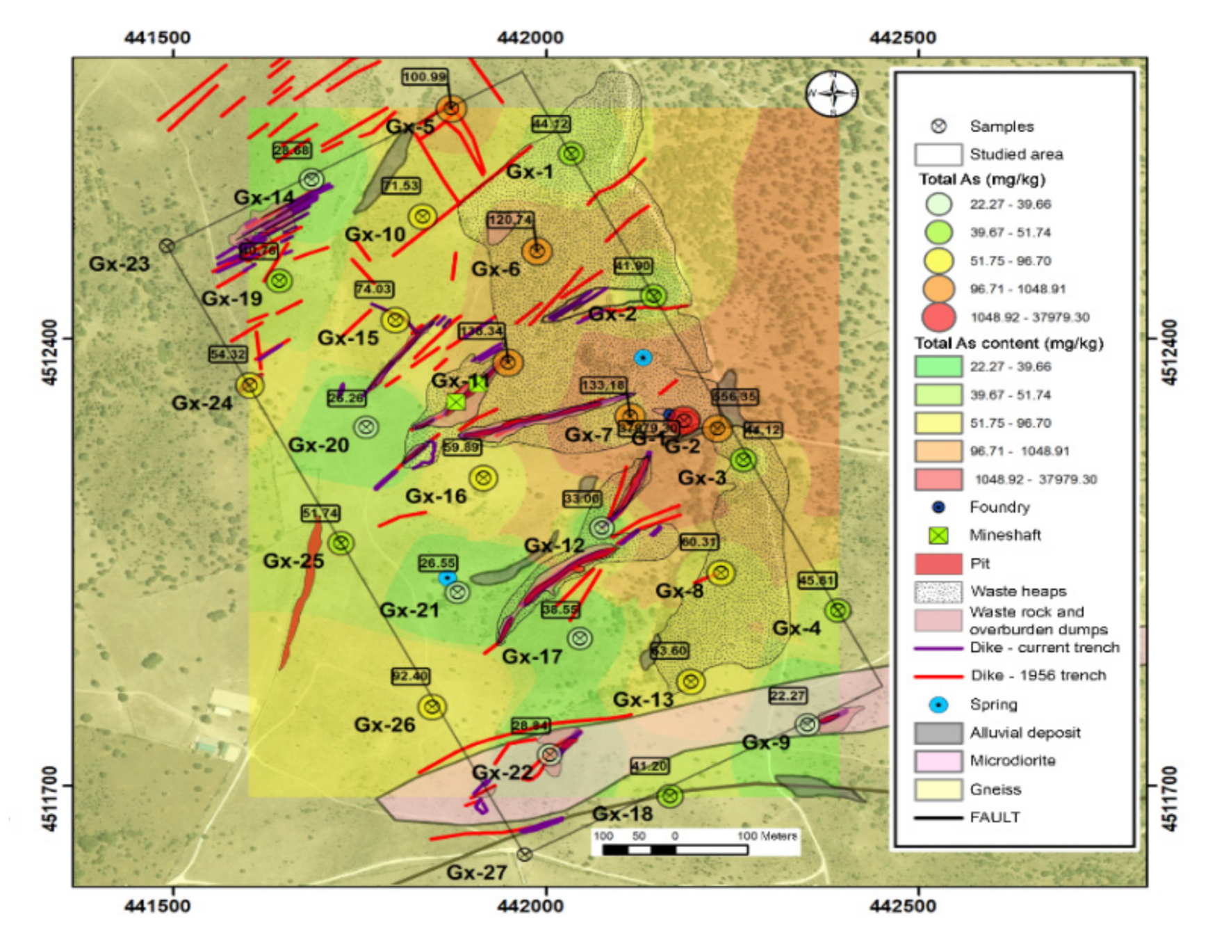
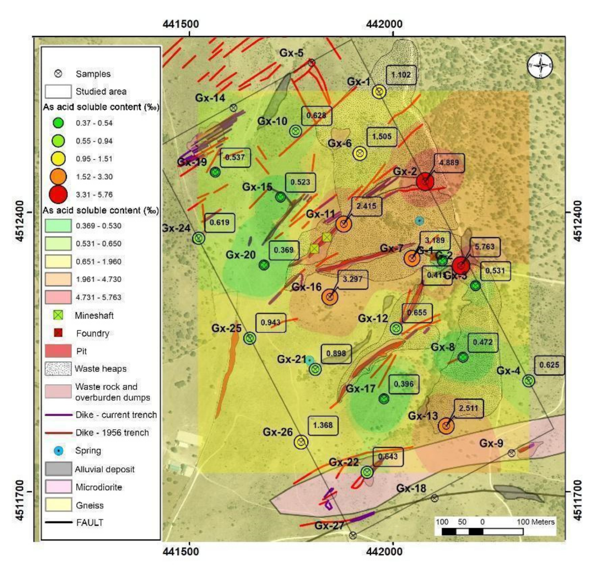
4.1. Geochemistry of Soil Samples

Soil samples show slightly acidic conditions, with an average pH value of 5 (Table 1). Figure 3 shows that the most acidic points coincide with the mine tailing dump and sediments downstream.
As regards the EC results (Table 1), soil samples show low electrical conductivity, with mean values of 780 µS cm−1, values of "normal soils", according to the American classification of soils (Soil Taxonomy), or not saline (EC < 2000 µS cm−1).
The average total arsenic content was 1482 mg kg−1, noting that there is a high variation in the content of this element, ranging from 22 mg kg−1 to 37969 mg kg−1 (Table 1).
The distribution of this element in the area shows that the higher concentrations of arsenic were found in areas occupied by dumps and fillings in the topographically low areas, where leachates can be washed away. On the other hand, in the higher areas and the intrusion of microdiorites, the arsenic concentration values are lower. Figure 4 summarizes the total arsenic content related to the environmental liabilities of mining.
Acid soluble contents suggest that arsenic leaching is low. The average value was 1.5‰ and the median was 0.65‰ (Table 1). The highest mobilization is found in G1 and GX02 with 5.7% and 4.9%, respectively. These points were located at an alluvial area and in the lower part of an anthropic fill.
The spatial representation of the results (Figure 5) shows that, on the whole, the arsenic, in the topographically lower parts, has the greater facility to be mobilized in an acidic medium, due to the presence of less resistant mineral phases. On the other hand, in the tailing dump, the extractable fraction is low because the arsenic is probably in the form of scorodite, which is poorly soluble under these conditions.
The contamination factor (CF) values for As are intermediate-high in almost all samples, regardless of their distance to the contamination sources. Even so, the highest values are found in areas close to tailing dumps. Furthermore, when the possible mobilization produced by mixing with acid drainage waters is assessed, the results obtained suggest a low potential risk for all samples. With the combination of the aforementioned factors, according to the matrix represented in Table 2, we obtain the qualitative assessment of environmental risk.
Our results are summarized in Figure 6 and suggest that the risk posed by these soils is moderate even if the degree of contamination is high, because the low mobility of arsenic prevents its dispersion. It is observed that the areas that present the greatest environmental risk are, in general, those covered by dumps and fillings from mining activity and, especially, those located downstream, highlighting the area of the smelter and attached dump and alluvial sediments from the stream that collects the drainage of these areas.

4.2. Geophysical Results

First, the distribution of apparent resistivity values (ρap) will be described by means of maps at the three depths of analysis (Figure 7). Then the results of the tomographic inversions are shown crossing the main resistivity anomalies (Figure 8).

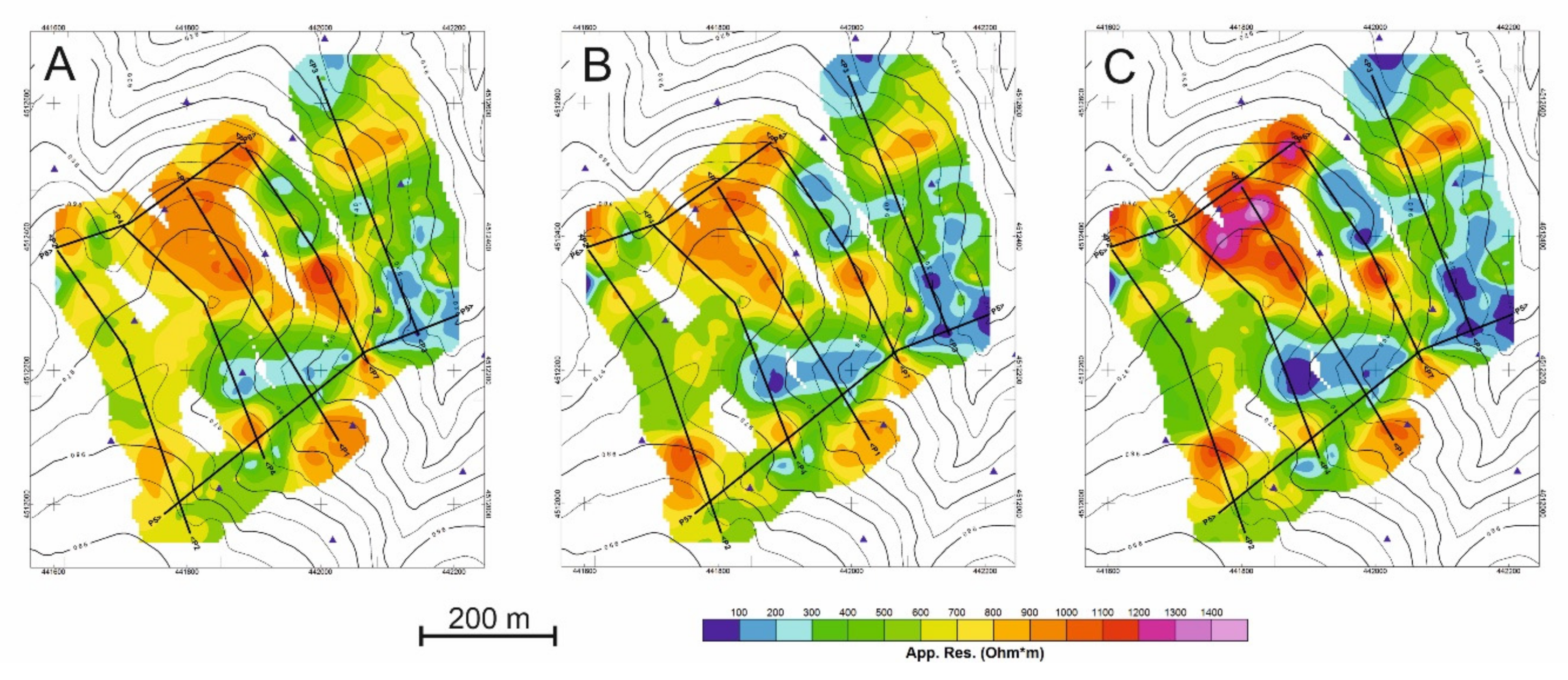
4.2.1. Apparent resistivity results
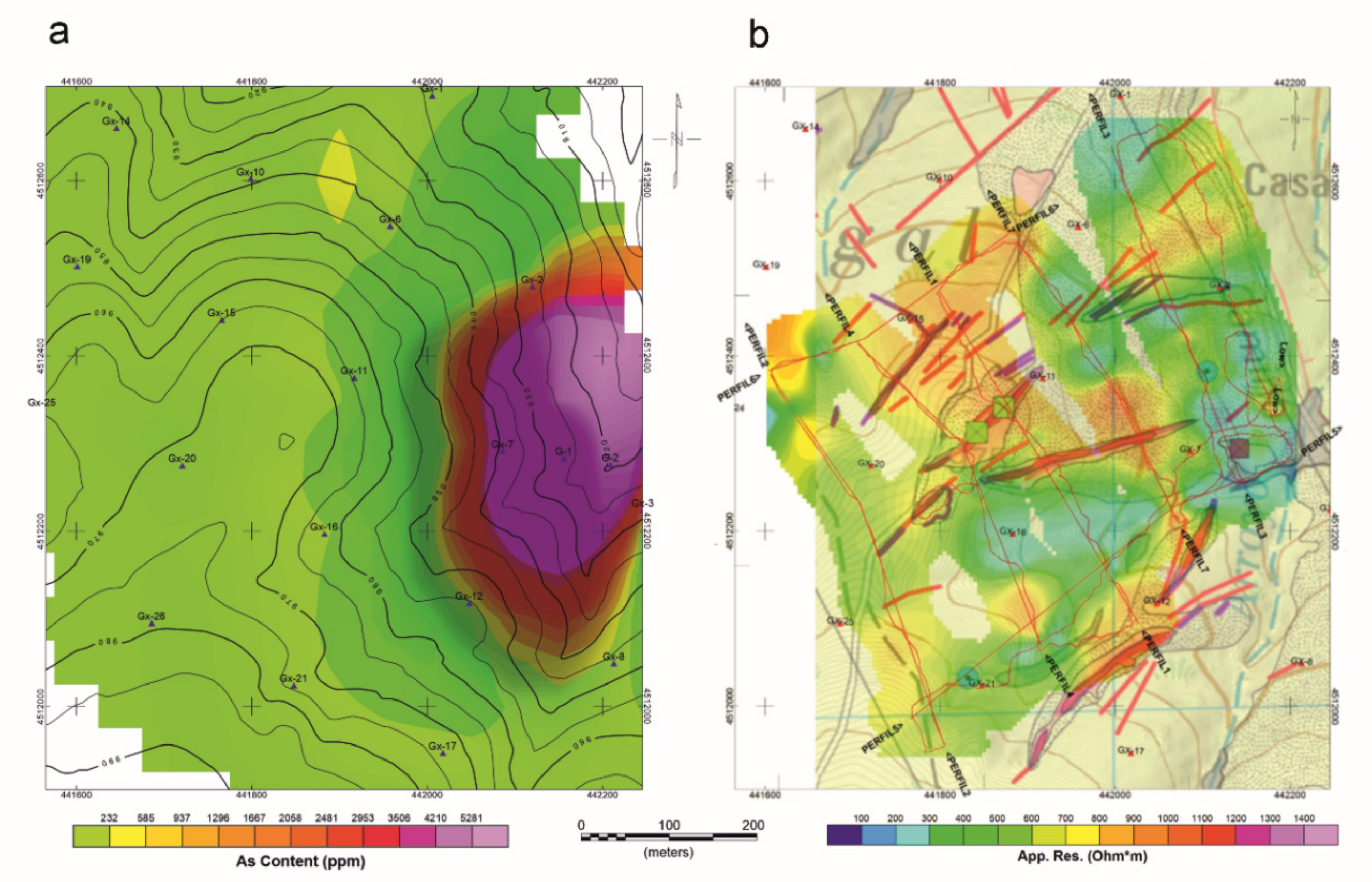
The distribution of the apparent resistivity values at the three depths of analysis is summarized in Figure 7.
The three resistivity maps show a similar pattern in the apparent resistivity distribution. Moreover, three groups of apparent resistivity values are distinguished (Figure 7).
(a)
The first group has values lower than 350 Ω m, reaching ρap values of 44 Ω·m. These values correspond to areas where clay and/or water are concentrated and coincide with the greatest development of natural soil, highly altered rock, and/or deposits resulting from anthropic activity. Its distribution extends in the ENE-WSW direction, which corresponds to a topographically depressed area, and in depth, this distribution is better defined with lower resistivity values.
(b)
The second group (ρap ranging from 350 to 750 Ω·m) indicates areas of intermediate apparent resistivity corresponding to weathered rock and/or soil.
(c)
The third group (ρap> 750 Ω·m), reaches values greater than 1500 Ω·m and corresponds to unaltered rock. These values are generally found in elevated areas with rocky outcrops with an ENE-WSW orientation but defined for lower resistivity value.
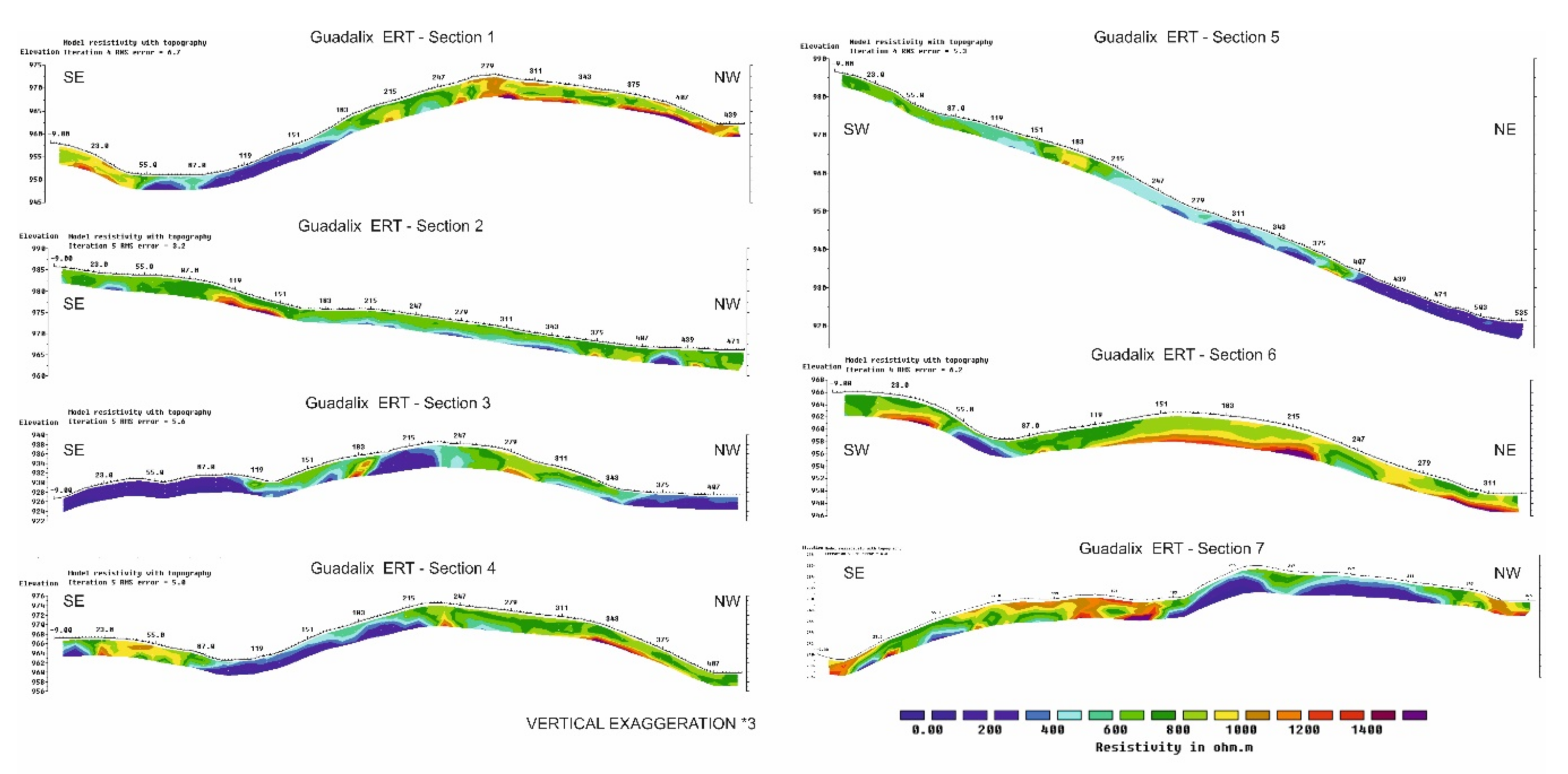
Once the apparent resistivity maps have been analyzed, seven cross-sections of the valley and the main mineralized zones were selected (Figure 8).
Along these sections, the apparent resistivity values at three depths were sampled every 5 m. Figure 9 shows the results of real depth resistivity obtained for the sections. Taking into account that the real resistivity values are always more contrasted than the apparent resistivity, which represents “average” values of the area irradiated by the EM field generated by the antenna, in real resistivity, three groups are distinguished:
(a)
The first group ranges from 0 to 400 Ω·m, indicating areas of high conductivity and therefore low resistivity. These characteristics correspond to soils with high amounts of clay and/or the presence of water. These areas are usually found in small valleys, where accumulations of arsenic leached by water can be found. In some cases, areas with low resistivity correspond to areas of fracture in the gneisses.
(b)
The second group shows intermediate resistivities, ranging from 400 to 800 Ω·m) and correspond to weathered microdiorites and/or more developed soils. They are usually located close to the surface and with an average thickness lower than two meters.
(c)
The third group shows high resistivity values (from 800 to 1400 Ω·m) which correspond to the presence of fresh rock (gneisses) as well as mineralized quartz dikes. They are usually found in the elevated areas and below the soils, although in some sections there are lateral contacts with conductive areas, probably fractures.

4.2.2. D resistivity distribution

For a better understanding of the spatial distribution of real resistivities, the results obtained from the tomographic inversion were interpolated to a 3D voxel model. This 3d model has an element size of 5 × 5 × 1 m and allows complete spatial visualization of resistivity values. The results of the model are summarized in Figure 10 and allow us to visualize a general trend ENE-WSW in the lower resistivity values.
These zones present a higher content of clay and/or water and are found along small valleys and fracture zones. In contrast, high resistivity values coincide with rock outcrops with very little or undeveloped soils. The spatial distribution follows the general ENE-WSW trend but dominating the most elevated areas.
Considering the geochemical and geophysical results together, the geochemical maps (Figure 11a and Figure 1b) show that high arsenic contents coincide with areas of very low resistivity, found in the foundry dump area. The topographically depressed zones (with strong structural control) with preferential direction ENE-WSW, show high potential natural accumulation of arsenic. These areas correspond to developed soils, anthropic accumulations, and fracture zones.

5. Conclusions

The analyzed area is contaminated by arsenic, as a result of the mining activity carried out in the zone. The highest concentrations of arsenic are located in topographically depressed areas, in anthropic deposits, and/or in highly developed soils.
The geophysical results allow us to obtain, clearly, the distribution of the anthropic surface deposits and soils, the fresh rock, as well as the conductive fracture zones.
This approach suggests that the application of geophysics and geochemistry provides valid support for the proper characterization of highly contaminated areas by PTEs.
In addition, the presence of conductive fractures in depth suggests the possible circulation of contaminants through them, as well as the preferred lines of circulation.
Furthermore, the results suggest that electrical resistivity tomography can be successfully adopted to define the extent of contaminated layers cost-effectively.
We argue that this information permits us to locate areas of the greater potential risk of contamination by As in an economic and simple economically and simply and to design geochemical sampling campaigns (Figure 11a,b).
Finally, it would be advisable to extend the study of arsenic contamination and potential mobilization of arsenic to the area of the reservoir for human supply using the proposed approach.

Author Contributions

Conceptualization, M.L.G.-L., E.C.-F., A.M.-M., P.C.; methodology, J.R.-R. and A.M.-M.; software, J.R.-R. and A.M.-M.; validation, M.L.G.-L., E.C.-F. and P.C.; formal analysis, M.L.G.-L., E.C.-F., P.C. and A.M.-M.; investigation, J.R.-R., M.L.G.-L., P.C., E.C.-F. and A.M.-M.; data curation, J.R.-R. and A.M.-M.; writing—original draft preparation, M.L.G.-L., P.C., E.C.-F. and A.M.-M.; writing—review and editing, M.L.G.-L., P.C., E.C.-F. and A.M.-M.; visualization, M.L.G.-L., P.C., E.C.-F. and A.M.-M.; supervision, M.L.G.-L.; P.C., E.C.-F. and A.M.-M. All authors have read and agreed to the published version of the manuscript.

Funding

This research received no external funding.

Acknowledgments

Comunidad de Madrid, CARESOIL-CM (S2013/MAE-2739).

Conflicts of Interest

The authors declare no conflict of interest.

References

  1. Paul, S.; Chakraborty, S.; Ali, N.; Ray, D. Arsenic distribution in environment and its bioremediation: A review. Int. J. Agric. Environ. Biotechnol. 2014, 8, 189. [Google Scholar] [CrossRef]
  2. Smith, E.; Naidu, R.; Alston, A. Arsenic in the Soil Environment: A Review. Adv. Agron. 1998, 64, 149–195. [Google Scholar] [CrossRef]
  3. Anthony, J.W.; Bideaux, R.A.; Bladh, K.W.; Nichols, M.C. Handbook of Mineralogy; Mineral Data Publishing: Tucson, AZ, USA, 2003. [Google Scholar]
  4. Gomez-Gonzalez, M.A.; Serrano, S.; Laborda, F.; Garrido, F. Spread and partitioning of arsenic in soils from a mine waste site in Madrid province (Spain). Sci. Total. Environ. 2014, 500, 23–33. [Google Scholar] [CrossRef] [PubMed]
  5. García-Lorenzo, M.L.; Marimón, J.; Navarro-Hervás, M.C.; Pérez-Sirvent, C.; Martínez-Sánchez, M.J.; Molina-Ruiz, J. Impact of acid mine drainages on surficial waters of an abandoned mining site. Environ. Sci. Pollut. Res. 2016, 23, 6014–6023. [Google Scholar] [CrossRef] [PubMed]
  6. Migaszewski, Z.M.; Gałuszka, A.; Dołęgowska, S. Arsenic in the Wiśniówka acid mine drainage area (south-central Poland) – Mineralogy, hydrogeochemistry, remediation. Chem. Geol. 2018, 493, 491–503. [Google Scholar] [CrossRef]
  7. Zawierucha, I.; Nowik-Zajac, A.; Malina, G. Selective Removal of As(V) Ions from Acid Mine Drainage Using Polymer Inclusion Membranes. Minerals 2020, 10, 909. [Google Scholar] [CrossRef]
  8. Tokoro, C.; Kadokura, M.; Kato, T. Mechanism of arsenate coprecipitation at the solid/liquid interface of ferrihydrite: A perspective review. Adv. Powder Technol. 2020, 31, 859–866. [Google Scholar] [CrossRef]
  9. Higueras, P.L.H.; Oyarzun, R.; Iraizoz, J.; Lorenzo, S.M.; Esbri, J.M.; Martinezcoronado, A. Low-cost geochemical surveys for environmental studies in developing countries: Testing a field portable XRF instrument under quasi-realistic conditions. J. Geochem. Explor. 2012, 113, 3–12. [Google Scholar] [CrossRef] [Green Version]
  10. Osinowo, O.O.; Falufosi, M.O.; Omiyale, E.O. Integrated electromagnetic (EM) and Electrical Resistivity Tomography (ERT) geophysical studies of environmental impact of Awotan dumpsite in Ibadan, southwestern Nigeria. J. Afr. Earth Sci. 2018, 140, 42–51. [Google Scholar] [CrossRef]
  11. Passaro, S.; Gherardi, S.; Romano, E.; Ausili, A.; Sesta, G.; Pierfranceschi, G.; Tamburrino, S.; Sprovieri, M. Coupled geophysics and geochemistry to record recent coastal changes of contaminated sites of the Bagnoli industrial area, Southern Italy. Estuarine, Coast. Shelf Sci. 2020, 246. [Google Scholar] [CrossRef]
  12. Villaseca, C.; Merino, E.; Oyarzun, R.; Orejana, D.; Perezsoba, C.; Chicharro, E. Contrasting chemical and isotopic signatures from Neoproterozoic metasedimentary rocks in the Central Iberian Zone (Spain) of pre-Variscan Europe: Implications for terrane analysis and Early Ordovician magmatic belts. Precambrian Res. 2014, 245, 131–145. [Google Scholar] [CrossRef]
  13. Capote, R.; Casquet, C.; Fernández Casals, M.J. La tectónica hercínica de cabalgamientos en el Sistema Central español. Cuad Geol Ibérica 1981, 7, 455–469. (in Spanish). [Google Scholar]
  14. Navidad, M.; Castiñeiras, P. Early Ordovician magmatism in the northern Central Iberian Zone (Iberian Massif): New U-Pb (SHRIMP) ages and isotopic Sr-Nd data. In Ordovician of the World; Gutiérrez-Marco, J.C., Rábano, I., García-Bellido, D., Eds.; IGME: Madrid, Spain, 2011; pp. 391–398. [Google Scholar]
  15. Pérez González, A.; Ruiz García, C.; Rodríguez Fernández, L.R. Torrelaguna Mapa Geológico de España, Escala 1:50000 1990, 509: 130 pp. (in Spanish). Available online: https://info.igme.es/cartografiadigital/geologica/Magna50Hoja.aspx?Id=509&language=es (accessed on 11 December 2020).
  16. González del Tánago Chanrai, J.; González del Tánago del Río, J. Minerales y Minas de Madrid; Consejería de Medio Ambiente: Mundi-Prensa, Madrid, 2002; 271p. (in Spanish) [Google Scholar]
  17. Recio-Vazquez, L.; Garcia-Guinea, J.; Carral, P.; Álvarez, A.M.; Garrido, F. Arsenic Mining Waste in the Catchment Area of the Madrid Detrital Aquifer (Spain). Water, Air, Soil Pollut. 2010, 214, 307–320. [Google Scholar] [CrossRef]
  18. ISO 10381-1: 2002. Soil Quality. Sampling. Part 1. Guidance on the Design of Sampling Programmes. Available online: https://www.aenor.com/normas-y-libros/buscador-de-normas/une/?c=N0039566 (accessed on 11 December 2020).
  19. ISO 17586: 2016. Soil Quality-Extraction of Trace Elements using Dilute Nitric Acid. Available online: https://www.iso.org/standard/60060.html#:~:text=ISO%2017586%3A2016%20specifies%20a,soils%20and%20soil%20like%20materials (accessed on 11 December 2020).
  20. García-Lorenzo, M.L.; Pérez-Sirvent, C.; Molina-Ruiz, J.; Martínez-Sánchez, M.J. Mobility indices for the assessment of metal contamination in soils affected by old mining activities. J. Geochem. Explor. 2014, 147, 117–129. [Google Scholar] [CrossRef]
  21. Li, J.; Kosugi, T.; Riya, S.; Hashimoto, Y.; Hou, H.; Terada, A.; Hosomi, M. Pollution potential leaching index as a tool to assess water leaching risk of arsenic in excavated urban soils. Ecotoxicol. Environ. Saf. 2018, 147, 72–79. [Google Scholar] [CrossRef] [PubMed]
  22. Usese, A.; Chukwu, O.L.; Rahman, M.M.; Naidu, R.; Islam, S.; Oyewo, E.O. Enrichment, contamination and geo-accumulation factors for assessing arsenic contamination in sediment of a Tropical Open Lagoon, Southwest Nigeria. Environ. Technol. Innov. 2017, 8, 126–131. [Google Scholar] [CrossRef]
  23. Ramírez-Pérez, A.; Álvarez-Vázquez, M. Ángel; De Uña-Álvarez, E.; De Blas, E. Environmental Assessment of Trace Metals in San Simon Bay Sediments (NW Iberian Peninsula). Minerals 2020, 10, 826. [Google Scholar] [CrossRef]
  24. Jiménez Ballesta, R.; Conde Bueno, P.; Martín Rubí, J.A.; García Giménez, R. Geochemical background levels and influence of the geological setting on pedogeochemical baseline concentrations of trace elements in selected soils of Castilla-La Mancha (Spain). Estudios Geológicos 2010, 66, 123–130. [Google Scholar] [CrossRef]
  25. Dentith, M.; Mudge, S.T. Geophysics for the Mineral Exploration Geoscientist; Cambridge University Press: Cambridge, England, UK, 2014. [Google Scholar]
  26. Reynolds, J.M. An Introduction to Applied and Environmental Geophysics; John Wiley and Sons: Hoboken, New Jersey, USA, 2011. [Google Scholar]
  27. Loke, M.; Barker, R. Rapid least-squares inversion of apparent resistivity pseudosections by a quasi-Newton method1. Geophys. Prospect. 1996, 44, 131–152. [Google Scholar] [CrossRef]
  28. Loke, M.H. Topographic modelling in resistivity imaging inversion. In Proceedings of the 62nd EAGE 968 Conference and Technical Exhibition, Glasgow, Scotland, England, UK, 29 May–2 June 2000. [Google Scholar]
  29. Loke, M.; E Chambers, J.; Rucker, D.F.; Kuras, O.; Wilkinson, P.B. Recent developments in the direct-current geoelectrical imaging method. J. Appl. Geophys. 2013, 95, 135–156. [Google Scholar] [CrossRef]
Figure 1. Geological sketch of the Spanish Central System (modified from [14] with the location of the study area and its geological map [15]. The coordinate system is ETRS89/UTM zone 30N (N-E). The position of the Central Iberian Zone (CIZ) in the Iberian Massif is shown in the upper part of the figure.
Minerals 10 01130 g001
Figure 2. (a) Geochemical sampling design. (b) Topographic map of the study area with the position of the data obtained with the CGM in Low mode (red) and in "high" mode (black line). The yellow points show the position where the tomographic inversions of the apparent resistivities have been made. The blue triangles correspond to the position of the geochemical samples.
Minerals 10 01130 g002
Figure 3. pH results in soil samples.
Minerals 10 01130 g003
Figure 4. Total arsenic content.
Minerals 10 01130 g004
Figure 5. Potential mobilizable arsenic content in acidic medium.
Minerals 10 01130 g005
Figure 6. Qualitative assessment of environmental risk results.
Minerals 10 01130 g006
Figure 7. Apparent resistivity (ρap) maps obtained at (A) 1.1 m depth, (B) 2.2 m depth, and (C) 3.3 m depth.
Minerals 10 01130 g007
Figure 8. Location of the profiles where the tomographic resistivity inversion has been conducted.
Minerals 10 01130 g008
Figure 9. Tomography resistivity inversion of the 7 sections represented in Figure 8. All sections have the same color scale and an ×3 vertical exaggeration.
Minerals 10 01130 g009
Figure 10. Spatial distribution of real resistivities obtained from tomography inversion. (a) ρ values > 700 Ω m, (b) ρ values < 500 Ω m.
Minerals 10 01130 g010
Figure 11. (a) Geochemical and (b) Geophysical results.
Minerals 10 01130 g011
Table 1. Geochemical results.
pHElectrical Conductivity (dS/m)Total Content (mg/kg)Acid Soluble As (µg/g)
G-12.812,60037,979.315.7
G-24.51954556.43.2
Gx-15.577744.10.05
Gx-25.798541.90.2
Gx-35.371944.10.02
Gx-44.9123045.80.03
Gx-55.2770101.00.2
Gx-65.2815120.70.3
Gx-75.2771133.20.4
Gx-85.169760.30.03
Gx-95.078822.30.2
Gx-104.874771.50.04
Gx-115.1752138.40.3
Gx-125.272933.00.02
Gx-134.882663.60.2
Gx-144.680928.70.2
Gx-154.769574.00.04
Gx-165.675259.90.2
Gx-174.773238.50.02
Gx-185.276041.20.35
Gx-195.178040.70.02
Gx-205.576026.30.01
Gx-214.878026.50.02
Gx-225.4128828.80.02
Gx-245.480754.30.03
Gx-254.878751.70.05
Gx-265.678092.40.1
Table 2. Environmental risk assessment criteria.
Mobility Index (AMI)
LowModerateHigh
Contamination factor (CF)LowVery lowLowModerate
ModerateLowModerateHigh
HighModerateHighVery high
Very highHighVery highExtreme
Publisher’sNote: MDPI stays neutral with regard to jurisdictional claims in published maps and institutional affiliations.

