An Automated Method to Generate and Evaluate Geochemical Tectonic Discrimination Diagrams Based on Topological Theory

Abstract

Discrimination diagrams can be used to distinguish different tectonic settings of igneous rocks. To improve the quality and efficiency of the design of discrimination diagrams, an automatic design and assessment method for discrimination diagrams is proposed based on topology theory. The method is aimed at programming the traditional process of discrimination diagram design, enabling computers to simulate the visual discrimination process. It thus automatically designs tectonic setting discrimination diagrams by investigating all possible combinations of geochemical elements. In the experiment, analyses of 3803 gabbro samples were collected from three tectonic settings, including island arc, ocean island, and mid-oceanic ridge. Using the proposed method, we found thousands of discrimination diagrams with fields overlapping less than 10%. By analyzing these diagrams, the most critical elements (or element ratio pairs) are identified. Based on the result, the feasibility of using gabbroic rocks to discriminate between tectonic settings is illustrated and four representative discrimination diagrams, including the La/Y–Nb/Ba diagram, Nb/Sc–Sc/Ba diagram, Ba/Nb–Ba/Sc diagram, and La/Na₂O–Nb/Ba diagram, are recommended for use. This research supports the view that gabbroic rocks can also be used to discriminate between different tectonic settings. The method could also be applied to other rock types.

1. Introduction

Discriminating among different types of tectonic settings from the chemical components of magmatic rocks is a common method in geochemistry [1,2]. In previous studies, basalts were usually taken as the subjects for analysis. This is because, in the mantle plume theory, basalts are produced from the rapid cooling of magma and thus contain the information about their tectonic settings [3,4]. Since the first discrimination diagram for basalt was proposed by Pearce [5,6], discrimination diagram theory has received increasing attention and undergone rapid development [7,8,9,10].

With the development of geochemistry, researchers began to direct their attention to other types of rocks or minerals and hoped to obtain more profound insights [11,12,13]. For example, Verma et al. [14] designed 15 multidimensional diagrams to discriminate acid rocks. Sánchez-Muñoz et al. [12] proposed a P–Fe diagram to discriminate feldspars. Verma et al. [15] presented a multidimensional scheme to classify the magma types of altered igneous rocks. Gabbro, a basic intrusive rock, is widespread in the Earth’s crust. The chemical composition of gabbroic rocks (except for cumulate gabbros) are similar to those of basalts [16,17,18]. However, the petrogenesis of gabbroic rocks is more complicated than that of basalts, and the existing discrimination diagrams for basalts cannot be applied to discriminate among the different tectonic settings of gabbroic rocks. Compared with basalts, gabbroic rocks are difficult to be used to design discrimination diagrams. It is difficult to determine the elements which are suitable for designing a discrimination diagram because of the complex differentiation processes of gabbroic rocks. Moreover, there are many different elements in rock samples, making it challenging to design discrimination diagrams by exhausting all combinations of geochemical elements.

In recent years, some researchers have proposed using confidence ellipses in statistics to improve the quality and design efficiency of discrimination diagrams [19,20,21]. Confidence ellipses can make the design and evaluation processes of discrimination diagrams programmable. However, technically speaking, it does not accord with facts to assume that the regions of sample points in a discrimination diagram are elliptical. In most of the discrimination diagrams, the areas of sample points are not elliptical and are not even symmetrical shapes. Another design method for discrimination diagrams is based on the probability distribution functions of samples [22]. However, the distribution types or the parameters (for kernel density estimation) must be adjusted artificially, making it difficult to automatically design, evaluate, and search discrimination diagrams. Moreover, the probability distribution function method is easily affected by oversampling, and its results may be quite different from the observed results. Thus, there is still no good method to investigate all possible combinations of geochemical elements.

In this research, an automatic analytical method for optimal discrimination diagrams of tectonic settings is presented based on topology theory. It aims to make the traditional process of designing discrimination diagrams through visual observation programmable, and then to automatically design and evaluate numerous discrimination diagrams testing all combinations of geochemical elements, and finally to determine the optimal diagrams and critical elements or element ratios. The key to the method is to use topology theory to simulate the visual observation process. In Section 2 of the paper, the methodology of the study is discussed. In Section 3, a number of gabbroic rock samples collected from the PetDB and GEOROC databases are introduced, and their tectonic settings are carefully checked. After data filtering, an experiment is conducted with the proposed method. In the experiment, 455,650 diagrams are automatically generated and evaluated. Thousands of useful discrimination diagrams are found. The preliminary results indicate that using the chemical elements of gabbroic rocks to discriminate among different tectonic settings is feasible. Four representative discrimination diagrams, including the La/Y–Nb/Ba diagram, Nb/Sc–Sc/Ba diagram, Ba/Nb–Ba/Sc diagram, and La/Na₂O–Nb/Ba diagram, are discussed in detail.

2. Methodology

2.1. Overall Framework

The presented method is illustrated in Figure 1. There are five main steps:

(1) Determine the elements and element ratios. Element ratios are the ratios of any two elements; for example, TiO₂ and SiO₂ can be combined as TiO₂/SiO₂ and SiO₂/TiO₂. An element ratio should be regarded as a new element.

(2) Select nonzero data: a rock sample analysis may not contain some specific elements or the values of specific elements are effectively 0 or infinite (for element ratios). In this case the sample is not used to generate the corresponding discrimination diagrams.

(3) Design discrimination diagrams: project each pair of elements (or element ratios) of rock samples on Cartesian coordinates. For each type of tectonic setting, draw the region of the sample points based on the Delaunay triangulation technology. In this step, both linear coordinates and logarithmic coordinates are considered (see Section 2.3, Section 2.4 and Section 2.5).

(4) Evaluate discrimination diagrams: evaluate the diagrams generated in step (3) with the indicator named overlap. For a discrimination diagram, if the overlap of two tectonic setting regions is large, the diagram is considered ineffective (see Section 2.6).

(5) Analyze statistics: determine the optimal discrimination diagrams that have low overlaps and identify the corresponding elements or element ratio pairs.

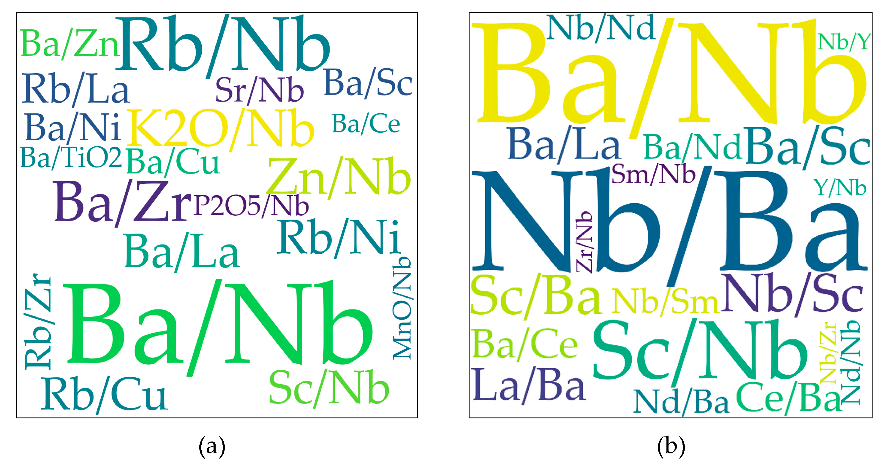
2.2. Element (or Element Ratio) Pairs

Our goal is to investigate all possible combinations of geochemical elements. Therefore, the first step is to combine the elements into element pairs and element ratio pairs. As mentioned in Section 2.1 (1), the element ratio pairs are treated as new elements for analysis. For example, if there are only three elements [a, b, c] in a rock, then 36 ($C_9^2$) element (element ratio) pairs can be generated from the set [a, b, c, a/b, a/c, b/a, b/c, c/a, c/b]. Inverse pairs such as (a/b, b/a) are discarded. Finally, 33 discrimination diagrams are designed and evaluated.

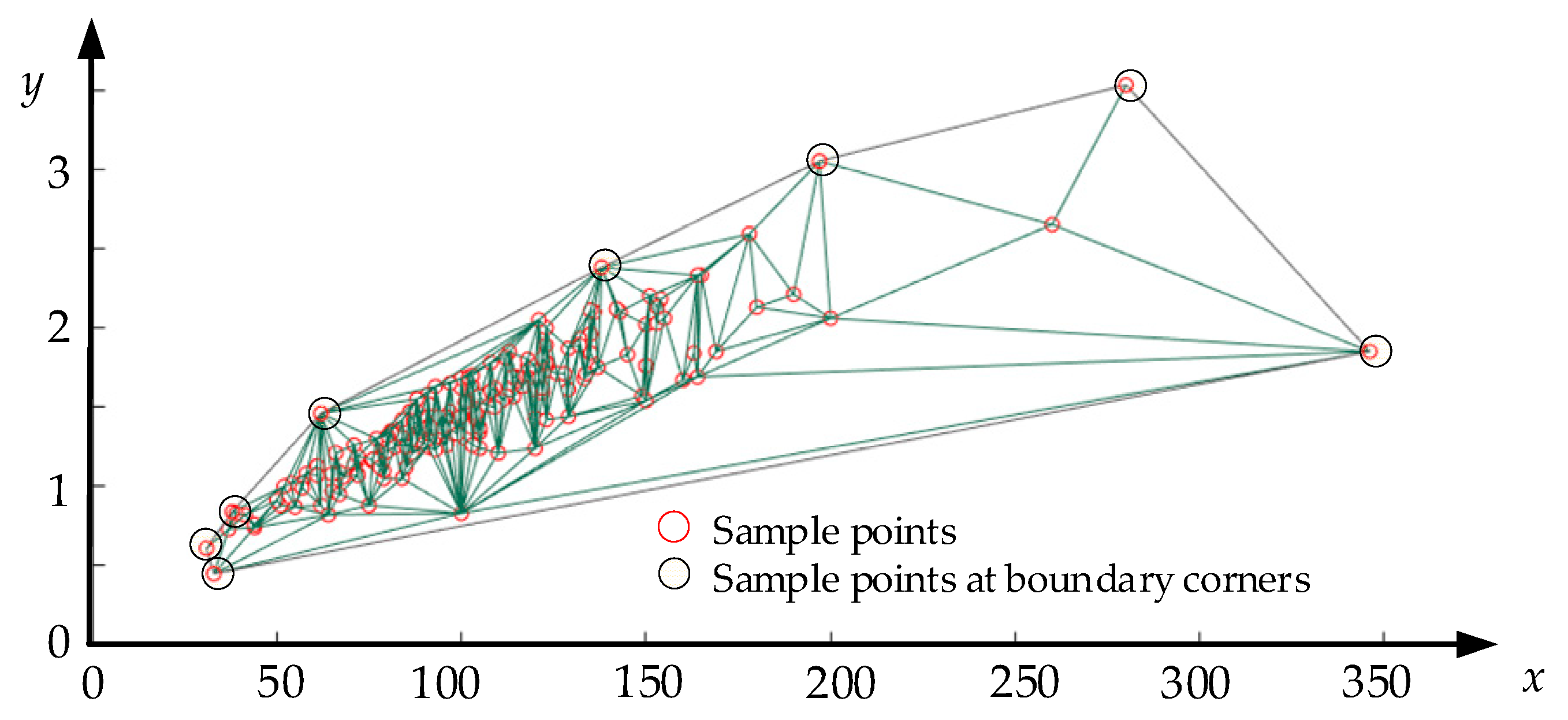
2.3. Delaunay Triangulation

Determining the region of samples means determining the region of the point cloud according to a specific confidence coefficient. For this purpose, Delaunay triangulation [23,24] is adopted. Delaunay triangulation is defined as a series of touching triangles that do not overlap with each other, and the region of the circumcircle of each triangle does not cover other triangles’ ices. Figure 2 shows an example of Delaunay triangulation. In this figure, all the points are interconnected by several dashed lines and then formed into a triangulation network. According to the Delaunay triangulation method, the connection mode of the points is unique, and a Delaunay triangulation always corresponds to a unique Voronoi polygon network [24], as shown in Figure 2.

The advantages of Delaunay triangulation are that it can present arbitrary shapes, make the triangles tend to equilateral triangles, and avoid generating “narrow” triangles as much as possible. The popular algorithms for generating Delaunay triangles include (1) a point-by-point insertion algorithm, (2) a triangle network growth algorithm, and (3) a divide-and-conquer algorithm. The first two algorithms are more popular than the third one because of their low computational overhead. Since there are many methods [25,26,27] explaining how to generate Delaunay triangulations, this process is not described in this paper.

Using Delaunay triangulation to determine the region of sample points can be illustrated in Figure 3. The region of a point cloud is a polygon (the outline of the triangulation network), and the boundary corner points are selected from the point cloud.

2.4. Coordinate Transformation of Samples

The coordinate transformation is the key to generating discrimination diagrams from the aspect of visual observation. This transformation consists of two parts: (1) coordinate transformation of different types of coordinates, and (2) coordinate transformation of multiscale coordinates.

2.4.1. Coordinate Transformation under Multiscale Coordinates

The importance of the ratio of the scale of the x-axis and the scale of the y-axis must be stressed because Delaunay triangulation is calculated based on Euclidean distances, and when the scale of the x-axis is different from the scale of the y-axis, the calculation process on a computer significantly differs from the results of visual observation. Taking Figure 4a as an example, the length of the x-axis is 0–10 and the length of the y-axis is 0–1. However, making the x-axis and the y-axis of equal length is convenient for visual observation. When designing a discrimination diagram, researchers tend to set the ratio of x-axis length and y-axis length as 1:1. For computers, however, the distribution of the points is illustrated in Figure 4b, and the Delaunay triangulation generated by these points is shown in Figure 4c. When projecting such a result onto custom coordinates, the result is shown in Figure 5a.

Most of the triangles in Figure 5a are clearly abnormal, and the confidence boundaries based on such a triangulation are not satisfactory for visual observation. Therefore, we propose to alter the scales of the points along the x or y direction to solve this problem:

$$\{\begin{array}{l}r=(y_{max}-y_{min})/(x_{max}-x_{min})\hfill \\ \begin{array}{ll}(x_i^{\prime },y_i^{\prime })=(r{x}_i,y_i)\hfill & i=1,2,\dots ,n\hfill \end{array}\hfill \end{array}$$

(1)

where, y_max and y_min are the maximum and minimum of the points along the y-axis and x_max and x_min are the maximum and minimum of the points along the x-axis. (x_i, y_i) is the original value of the ith point, and (x_i’, y_i’) is the zoomed valued of the ith point. By generating a Delaunay triangulation with the zoomed points, a set of connection rules for the points can be calculated. After this step, by connecting the original points according to these connection rules, a new triangulation can be made, as shown in Figure 5b. It is evident that Figure 5b is more consistent with the visual observation.

2.4.2. Coordinate Transformation under Linear and Logarithmic Coordinates

In geochemistry, two types of coordinate are usually used: linear coordinates and logarithmic coordinates [28]. As is well known, the visual effects vary with the types of coordinates, as shown in Figure 6. Therefore, when using computer vision technology to plot the sample points, it is necessary to take both linear and logarithmic coordinates into consideration. The method of coordinate transformation is as follows: (1) when using linear coordinates to design a discrimination diagram, the altered samples are directly projected onto a linear coordinate system, the boundary corner points are then determined using the algorithm in Section 2.5, and finally, the confidence region is established by connecting the corner points; (2) when using logarithmic coordinates for design, (a) a set of “pseudo samples” is generated by calculating the logarithms of the altered data, (b) the pseudo samples are projected onto a linear coordinate system, (c) the boundary corner points of the pseudo samples are set according to the algorithm in Section 2.5, and (d) the real samples that correspond to the pseudo boundary corner points are determined and connected to generate the confidence region.

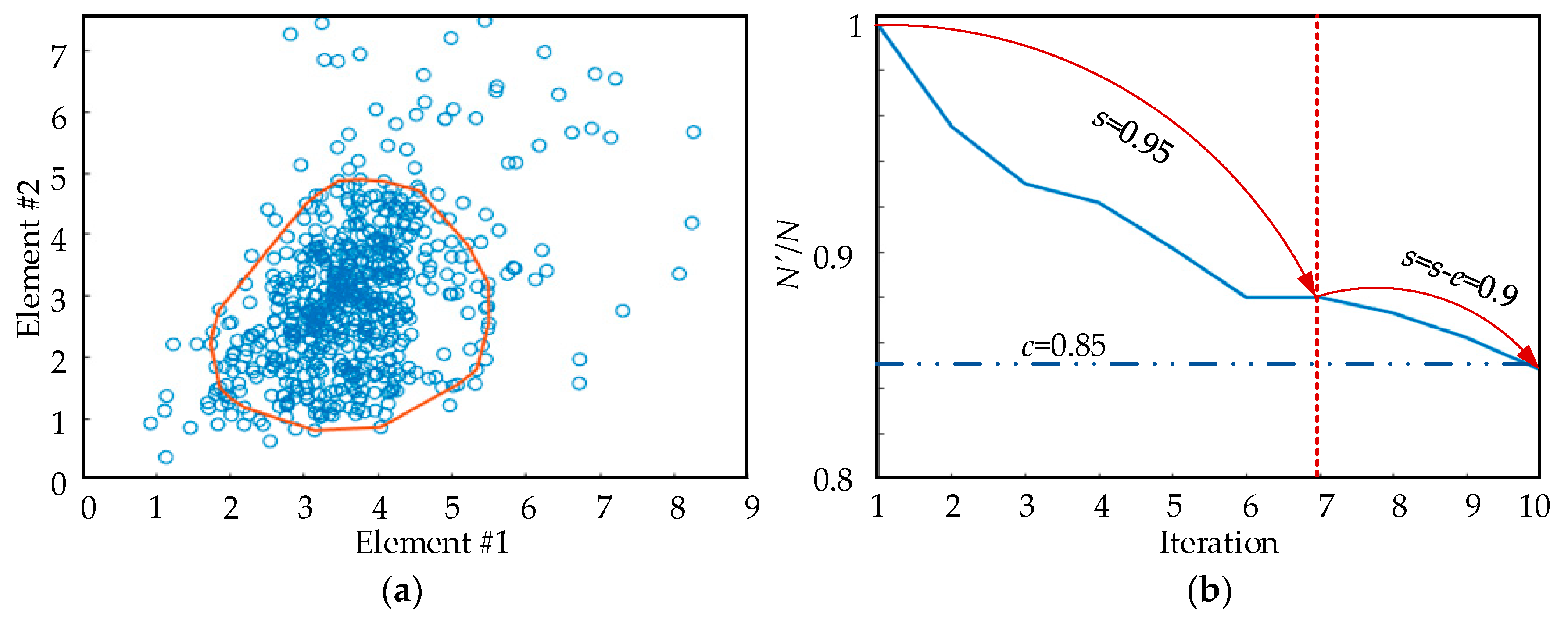
2.5. Confidence Region

When determining the region of sample points, the most important issue is how to determine the confidence coefficient and use the confidence coefficient to set a confidence region. In other words, it is necessary to select the normal points to generate a triangulation mesh and remove the abnormal (outlying) points. As Delaunay triangulation can maximize the minimum angle of a triangle, a data elimination method is proposed based on the size of triangles to filter out abnormal sample points and determine confidence regions. The flow chart is shown in Figure 7.

For a specific confidence coefficient, c, the algorithm removes the abnormal samples iteratively to make the proportion of remaining samples meet c. A reduction ratio, s, and an adjustment factor of the reduction ratio, e, are proposed to control the number of abnormal samples in each iteration. The value of s determines the number of triangles that are filtered out in every iteration, and the value of e is used to dynamically adjust the value of s to keep the algorithm from an endless loop.

After initializing the parameters, an initial Delaunay triangulation of the whole point cloud is first generated. As mentioned above, Delaunay triangulation tends to produce equilateral triangles as much as possible, and when there is an abnormal point, the corresponding triangle is large or spindly. By this rule, the abnormal points are removed by eliminating the large and spindly triangles. The strategy we take is to sort all the triangles by their longest lines from longest to shortest, and then remove the first (1 − s) × 100% triangles. This process leaves some points isolated from the triangulation network, and the isolated points are considered abnormal points that need to be removed. After removing the abnormal points, a new Delaunay triangulation is generated with the remaining points; then, all the points covered by this triangulation are identified as the remaining points of this iteration. If the number of remaining points, N’, is equal to or less than N × c, then N’ can meet the requirement of c. If not, the algorithm moves on to the next iteration.

It should be noted that the reduction ratio, s, should be close to 1. Therefore, when the algorithm meets the inequality N’ ≤ N × c, it can be considered that N’ = N × c and the boundary of the current Delaunay triangulation can be regarded as the boundary of the points under the confidence coefficient, c. The boundary is the connection of some specific sample points. In addition, when the N’ in an iteration equals the N’ in the last iteration, it means that s is too large to be used to filter the points. In this case, the adjustment factor of reduction ratio, e, is applied to reduce the value of s.

Figure 8 is an example of using the iteration algorithm to calculate the confidence field. The value of c is set to 0.85, the s is set to 0.95, and e is set to 0.05. In the first six iterations, the algorithm filters the points with the initial parameters. At the seventh iteration, it can be seen that the N’/N ratio does not decrease. Then, in the next iteration, the value of s is adjusted by e. Finally, the N’/N ratio reaches the confidence coefficient at the 10th iteration. It should be noted that, generally, the N’/N ratio does not exactly equal c but is an approximation because the number of samples is a discrete value.

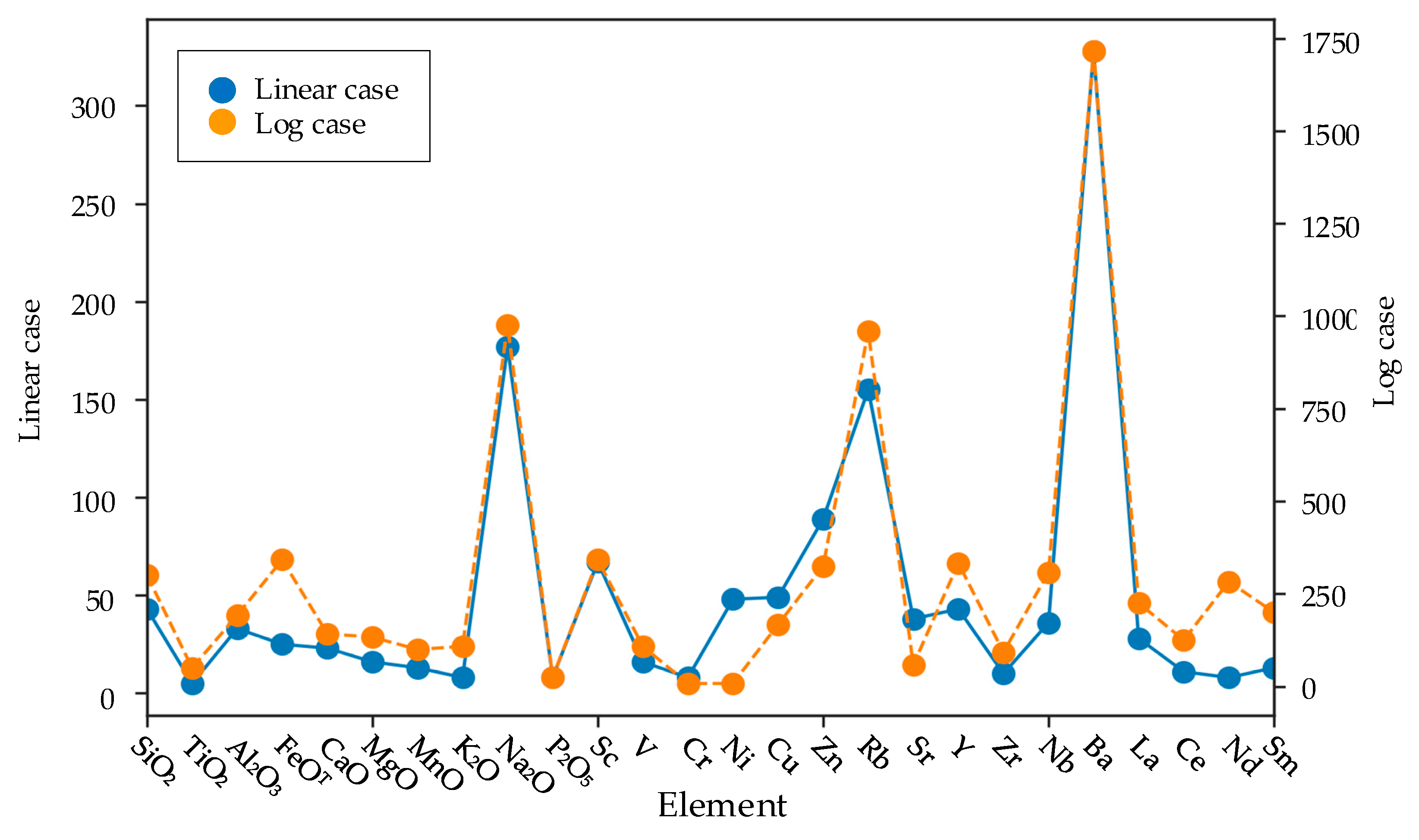
2.6. Evaluation of Discrimination Diagrams

The effectiveness of a discrimination diagram is evaluated by the overlap rate. Regardless of which type of coordinate system is used, low overlap represents high effectiveness. In this research, the overlap is defined as follows: suppose that there are n types of samples in a discrimination diagram; the overlap is given by:

$$\{\begin{array}{l}\begin{array}{cc}{\gamma }_i={\displaystyle \sum _{\begin{array}{c}j\in \left\{1,2,\dots ,n\right\}\\ j\ne i\end{array}}\frac{A(R_i\cap R_j)}{A(R_i)}},& i=1,2,\dots ,n\end{array}\hfill \\ \gamma =\frac{1}{n}{\displaystyle \sum _{k=1}^n{\gamma }_i}\hfill \end{array}$$

(2)

where R_i is the region of the ith type of samples, A(R_i) is the area of R_i, γ_i is the overlap rate of the region of the ith type of samples and other types of samples, and γ is the overlap rate of the whole discrimination diagram and is a value between [0,1]. Therefore, if the area of the overlap is large, the overlap rate is large.

3. Experiment and Analysis

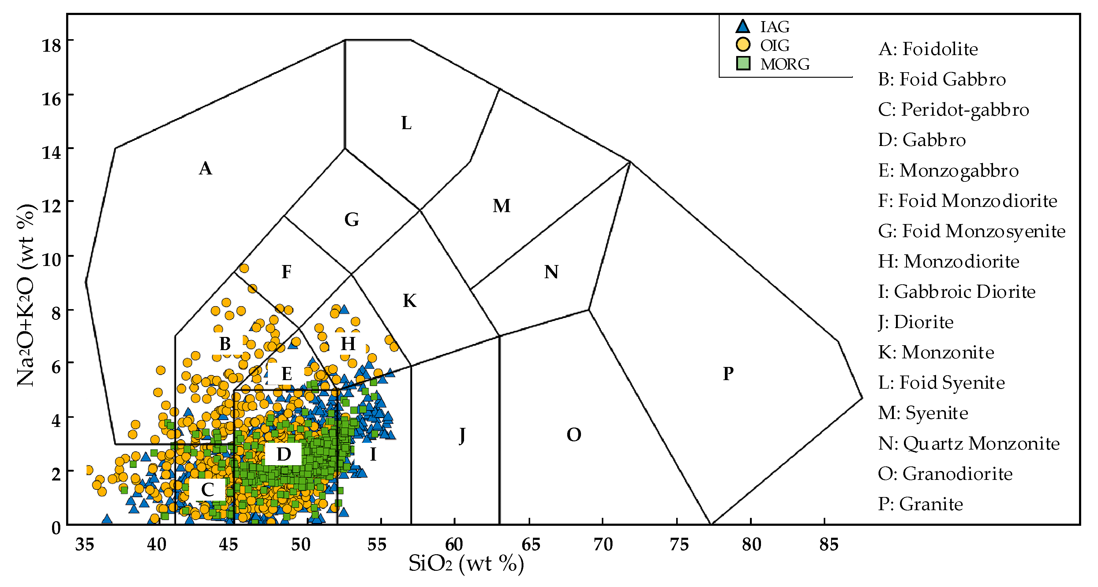
3.1. Data Collection and Preprocessing

The samples used in our experiment were 3803 gabbroic rock samples downloaded from PetDB [29] and GEOROC [30] databases. All the samples were divided into three types: island-arc gabbroic rocks (IAG), ocean-island gabbroic rocks (OIG), and mid-oceanic ridge gabbroic rocks (MORG). The distribution of the samples is illustrated in Figure 9. The numbers of IAG, OIG, and MORG were 743, 1668, and 837, respectively. Every sample contained data for 143 elements, including major elements, trace elements, and isotopes. The original data were filtered as follows.

First, all the data were transformed into the GEOROC format. Then, according to the names of the rock samples, the volcanic rocks, mantle xenoliths, dunite, dolerite, pyroxenite, sedimentary rocks, and metamorphic rocks were removed to ensure that remaining samples were gabbroic rocks, such as gabbro, anorthosite, norite, essexite, and troctolite. After this step, the samples with SiO₂ > 56 wt% or SiO₂ < 35 wt% were filtered out. Moreover, because the tectonic setting information for the samples was ambiguous (some samples were labeled with geomorphologic terms, for instance, seamount, submarine ridge, and convergent margin), we carefully checked all the samples according to the locations, longitudes and latitudes, and the analytical results provided by the contributors, and then divided them into the correct tectonic settings. In addition, it should be noted that we did not remove the cumulate gabbroic rocks, altered samples, or contaminated samples. Further, considering that there might be some uncertain influencing factors in the data set (for example, erroneous records), the box-plot approach was used to remove the outliers and ensure that the remainder of the samples accounted for 85% of the whole data set. Figure 10 shows the distributions of the remaining samples on the plutonic Total alkali–silica (TAS) diagram.

Some elements were not recorded for more than 40% of the samples, and we did not use them in the experiment. After filtering, 26 elements, including SiO₂, TiO₂, Al₂O₃, FeO^T, CaO, MgO, MnO, K₂O, Na₂O, P₂O₅, Sc, V, Cr, Ni, Cu, Zn, Rb, Sr, Y, Zr, Nb, Ba, La, Ce, Nd, and Sm were selected. The means and the standard deviations of the element contents for the three types of tectonic settings are presented in

Table 1. Mean element contents of island-arc gabbroic rocks (IAG), ocean-island gabbroic rocks (OIG), and mid-oceanic ridge gabbroic rocks (MORG) samples.

Basic Elements	IAG	OIG	MORG	Basic Elements	IAG	OIG	MORG
SiO2 (wt%)	47.9	46.5	49.6	Ni (ppm)	79.3	191	202
TiO2 (wt%)	0.933	2.17	0.812	Cu (ppm)	47.5	77.5	65.4
Al2O3 (wt%)	17.6	15.6	16.4	Zn (ppm)	77.0	75.0	52.7
FeOT (wt%)	9.10	9.78	6.81	Rb (ppm)	12.3	13.9	0.512
CaO (wt%)	11.4	12.1	12.0	Sr (ppm)	381	465	130
MgO (wt%)	8.11	8.70	9.64	Y (ppm)	15.3	19.2	15.7
MnO (wt%)	0.165	0.150	0.14	Zr (ppm)	44.4	111	31.3
K2O (wt%)	0.549	0.777	0.0762	Nb (ppm)	2.44	18.3	1.14
Na2O (wt%)	2.17	2.35	2.64	Ba (ppm)	157	181	9.59
P2O5 (wt%)	0.154	0.336	0.0890	La (ppm)	5.17	19.2	1.97
Sc (ppm)	39.1	28.1	33.9	Ce (ppm)	14.3	40.6	6.22
V (ppm)	261	269	177	Nd (ppm)	7.87	23.0	6.57
Cr (ppm)	272	468	300	Sm (ppm)	2.04	5.06	2.18

and

Table 2. Standard deviation of the element contents of IAG, OIG, and MORG samples.

Basic Elements	IAG	OIG	MORG	Basic Elements	IAG	OIG	MORG
SiO2 (wt%)	3.67	3.25	2.63	Ni (ppm)	91.5	211	277
TiO2 (wt%)	0.695	1.50	1.14	Cu (ppm)	35.1	71.2	39.0
Al2O3 (wt%)	3.83	4.60	3.09	Zn (ppm)	39.2	39.0	31.7
FeOT (wt%)	2.83	3.55	2.42	Rb (ppm)	17.9	19.5	0.570
CaO (wt%)	2.69	2.97	1.87	Sr (ppm)	243	345	44.8
MgO (wt%)	4.17	5.20	3.44	Y (ppm)	9.06	13.5	16.0
MnO (wt%)	0.0581	0.05	0.06	Zr (ppm)	38.7	110	38.3
K2O (wt%)	0.666	0.90	0.13	Nb (ppm)	2.83	22.7	2.33
Na2O (wt%)	1.05	1.20	0.85	Ba (ppm)	144	191	7.78
P2O5 (wt%)	0.163	0.43	0.25	La (ppm)	4.93	21.6	3.58
Sc (ppm)	21.5	12.5	13.2	Ce (ppm)	15.0	46.0	12.1
V (ppm)	124	156	125	Nd (ppm)	5.99	25.2	12.8
Cr (ppm)	418	600	363	Sm (ppm)	1.48	4.85	3.57

. In addition, the Mg# was calculated by Equation (3), and the result was 0.75.

$$\mathrm{Mg}\#=\frac{\mathrm{MgO}/40}{\mathrm{MgO}/40+\mathrm{Fe}{\mathrm{O}}^{\mathrm{T}}/72}$$

(3)

3.2. Designation and Evaluation of Discrimination Diagrams

Through permutations and combinations, 650 ($A_{26}^2$) element ratios were produced. Thus, there were 650 + 26 = 676 elements. Based on these elements, 227,825 ($C_{676}^2$ − 650/2) element (element ratio) pairs were found. Along with these pairs, there were two types of coordinate systems, so a total of 455,650 discrimination diagrams were designed and evaluated.

The parameters were set as follows: the confidence coefficient c was 85%, the reduction ratio s was 0.095, and the adjustment factor of the reduction ratio e was 0.01. The evaluation processes included four parts: (1) effectiveness of discriminating between IAG and non-IAG, (2) effectiveness of discriminating between OIG and non-OIG, (3) effectiveness of discriminating between MORG and non-MORG, and (4) effectiveness of discriminating among IAG, OIG, and MORG.

3.2.1. Discrimination Diagrams for IAG and Non-IAG

By analyzing all the overlap rates in all the discrimination diagrams, the effectiveness of discriminating between IAG and non-IAG was evaluated. The result showed that when using linear coordinates, there were 795 discrimination diagrams and that when using logarithmic coordinates, there were 260 discrimination diagrams whose overlap rates were less than 10%, and examples are shown in Figure 11.

Then, the word clouds of the top 20 elements (or element ratios) were produced according to their occurrence frequencies in the 795 linear discrimination diagrams and 260 logarithmic diagrams, as shown in Figure 12. It can be found from Figure 12a that Ba/Nb and Rb/Nb have the highest frequencies of occurrence in the linear diagrams, meaning that the two elements (including element ratios) have the most considerable effect on discriminating in linear cases. Similarly, Figure 12b indicates that Nb/Ba and Ba/Nb are the most important elements (including element ratios) for discriminating IAG and non-IAG using logarithmic coordinates.

For further analysis, we counted the frequencies of occurrence of the basic elements by decomposing all the element ratios, as shown in Figure 13. The result illustrates that Nb, Ba, Rb, La, and Sc have the highest frequencies in linear cases, meaning that these five elements contribute the most to the linear discrimination process; Ba, Nb, Sc, La, and Zn have the highest frequencies of occurrence in logarithmic cases, meaning that they are the most useful elements for logarithmic discrimination.

3.2.2. Discrimination Diagrams for OIG and Non-OIG

By analyzing all the overlap rates of OIG and non-OIG for all the discrimination diagrams, the effectiveness of discriminating between OIG and non-OIG was evaluated. With the proposed method, 276 linear discrimination diagrams and 82 logarithmic diagrams whose overlap was less than 1% were found. Examples are shown in Figure 14.

The word clouds of high-frequency elements (including element ratios) are illustrated in Figure 15. This figure indicates that Nb/Sc has a significant effect on discriminating between OIG and non-OIG for linear cases, and the element ratios comprised of Na₂O and Nb, Nb and Sm, Nb and Y are the most important elements (and element ratios) for logarithmic cases.

Moreover, by decomposing all the element ratios into basic elements, we find that Nb, Sc, Cu, La, and Ce have the highest frequencies in linear diagrams and that Nb, Sc, Sm, and Na₂O are the most significant basic elements in logarithmic diagrams, as shown in Figure 16.

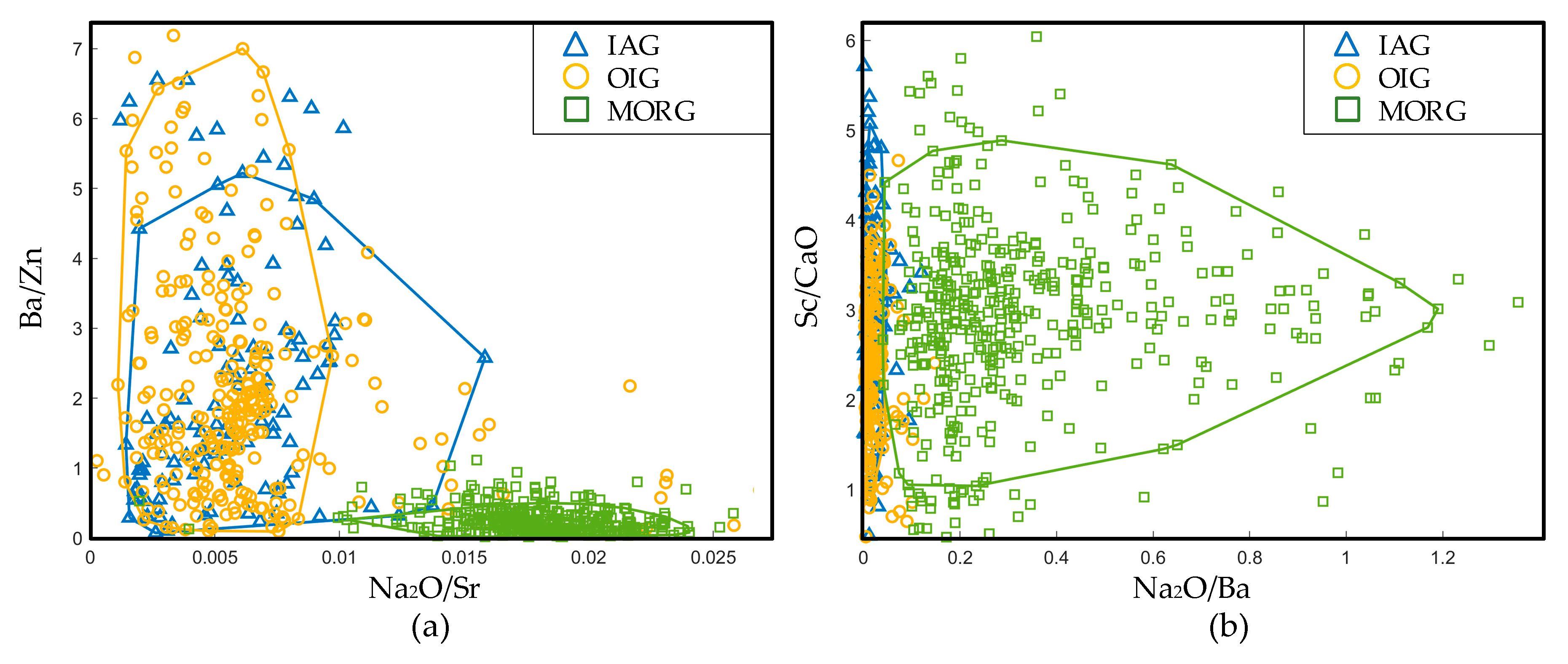
3.2.3. Discrimination Diagrams for MORG and Non-MORG

By analyzing the overlap rates of MORG and non-MORG fields in all the discrimination diagrams, the effectiveness of discriminating between MORG and non-MORG was evaluated. As a result, 276 linear discrimination diagrams and 1889 logarithmic discrimination diagrams whose overlap was less than 1% were found. Examples are shown in Figure 17.

The word cloud of the linear discrimination diagrams shows that Na₂O/Ba has the most significant effect on the discrimination process, as shown in Figure 18a; the word cloud of the logarithmic discrimination diagrams indicates that the element ratio pairs comprised by Na₂O and Ba, Na₂O and Rb are the most frequently occurring elements, as shown in Figure 18b.

In addition, Figure 19 indicates that Ba, Na₂O, Rb, Zn, and Sc contribute the most to linear discrimination, and that Ba, Na₂O, and Rb are the most effective elements in logarithmic discrimination.

3.2.4. Discrimination Diagrams for IAG–OIG–MORG

In this section, the discrimination diagrams that could discriminate among the three types of tectonic settings with overlaps of less than 10% were counted. The results showed that there are six acceptable linear discrimination diagrams and 124 acceptable logarithmic discrimination diagrams, and examples are shown in Figure 20.

Combining Figure 21 and Figure 22, it can be seen that (1) in linear cases, the element ratios of Nb and Sc are the most significant contributors and that Nb, Ba, and Sc are the most significant basic elements, while SiO₂, K₂O, Ni, Cu, La, and Ce also have certain effects on discrimination; (2) in logarithmic cases, the element ratios of Nb and Sc and of Ba and Sc contribute the most to the discrimination process and that Nb, Ba, and Sc are the most useful basic elements, while TiO₂, Al₂O₃, FeO^T, V, Cr, Ni, and Sr can slightly help to discriminate among different tectonic settings.

4. Discussion

4.1. The Use of Basalt in Discriminating among Different Tectonic Settings

Fundamental magmatic theory based on work with globally distributed basic rocks developed in the 1920s–1960s [32]. In the 1970s–1980s, because of results from marine geology and the implementation of deep-sea drilling projects and especially because of the establishment and improvement of the theory of plate tectonics, magmatic petrology (especially the basalt theory) developed rapidly [33]. In magmatic petrology, basic rocks are the most profoundly studied type of rock, and their data are available in great quantity with high quality. These studies established the foundation for the method and standard of using basalt to discriminate among different tectonic settings and significantly promoted the development of petrotectonics and geodynamics [33,34]. In the 1970s–1980s, with the rapid development of element analysis techniques, increasingly more major and trace elements could be precisely measured, which led to many theories and methods of discriminating among different tectonic settings with major and trace elements [35]. After Irvine and Barager [36] and Miyashiro [37] first designed several discrimination diagrams with some major elements, a group of scholars represented by Pearce summarized the relationship between the chemical components of basalts and tectonic settings based on statistical methods and proposed many discrimination diagrams [37,38,39,40,41,42,43,44,45,46,47,48,49,50,51,52,53]. All these achievements provided new approaches for research on plate tectonics and continental orogenic belts and pushed the studies of basalt to a peak. Designing a discrimination diagram requires a large number of samples. All the samples should be of high reliability and well-defined with their tectonic information. Therefore, using discrimination diagrams should be treated seriously [35,49].

Many studies show that the combination of elements of rock can reflect tectonic settings. Different tectonic settings correspond to diverse source and magmatic processes and different physicochemical conditions, thus leading to the variations among the combinations of elements (especially trace elements) of different tectonic settings. These studies provide the basis of designing discrimination diagrams with major and trace elements [35,49,54]. In a discrimination diagram, the regions of different tectonic settings are determined by many rock samples, and the samples should have been well-studied and clearly labeled with their tectonic information. Therefore, it is necessary to build a database for various rocks, especially for the well-studied and undisputed rock samples, to improve the discrimination diagrams. For example, the granite discrimination diagram proposed by Pearce et al. [27] is based on the trace element data of 600 precisely studied granite samples collected from a database of chemical elements of rocks.

4.2. Using Gabbroic Rocks in Discrimination Tasks?

In petrography, gabbroic rocks are composed of light-colored minerals such as plagioclase and the dark-colored minerals such as pyroxene, and olivine (and hornblende). The pyroxene includes clinopyroxene and orthopyroxene. If a gabbroic rock is composed of only plagioclase and orthopyroxene, it is a norite; if it is composed of only plagioclase and clinopyroxene, it is a narrowly defined as gabbro; if it is composed of only plagioclase and olivine, it is a troctolite; if it is mainly composed of plagioclase, it is an anorthosite [3,34]; if it is composed of plagioclase and hornblende, it may be a hornblende gabbro or a diorite according to the composition of the hornblende. Therefore, the gabbroic rocks sensu lato have a wide variety, and the chemical compositions of gabbroic rocks vary significantly. Thus, using gabbroic rocks to design discrimination diagrams is challenging.

As a kind of intrusive rock, gabbroic rocks exist in two forms: (1) cumulate gabbroic rocks that have a layered structure and (2) homogeneous gabbroic rocks that are composed of pyroxene and plagioclase, which result from residual magma. The compositions of cumulate gabbroic rocks are significantly different from those of basalts, while the compositions of homogeneous gabbroic rocks are generally similar to those of basalts [16,17]. As a gabbroic rock can be mainly composed of either cumulate rocks or residual magma, the compositions of gabbroic rocks are complex. The magmas that form gabbroic rocks may have experienced crystallization separation processes and mixing processes. Therefore, the basalt discrimination diagrams cannot always be applied to gabbroic rocks. Many researchers have studied the tectonic settings of gabbroic rocks with basalt discrimination diagrams; however, this application is not always suitable. Moreover, in the previous studies, there is no discrimination diagram specifically for gabbroic rocks.

It is evident that cumulate gabbros cannot be projected onto basalt diagrams because their compositions are distinctly different from those of basalts. For example, from the previous statistics, the average content of TiO₂ in MORB is 1.20–1.50%, the average content of TiO₂ in IAT is 0.80%, and the average content of TiO₂ is OIB more than 2.00% [31,47]. Generally, the content in TiO₂ of basalt is seldom less than 0.5%. Andesite is different, and its content of TiO₂ can be less than 0.5%. Moreover, the content of TiO₂ in boninite is less than 0.4% [55,56]. However, the content of TiO₂ in gabbroic rocks is generally low and can be as low as 0.2–0.3% [34]. This situation occurs because cumulate gabbroic rocks are mainly composed of cumulate minerals (olivine, pyroxene, and plagioclase) and interstitial melts that cool in the spaces between cumulate minerals, but these cumulate minerals do not contain Ti, and the Ti of gabbroic rocks mainly exists in the interstitial melts. However, the proportion of interstitial melt in gabbroic rock is uncertain, making the content of Ti decrease in varying degrees. If discriminating among different tectonic settings of gabbroic rocks with a basalt discrimination diagram based on Ti, all the gabbroic rock samples would be determined as island arc rocks, which is extremely unreasonable.

Some researchers think that homogeneous gabbroic rocks can be projected onto basalt discrimination diagrams because their compositions are similar to those of basalts [57,58], which is not entirely true. The texture characteristics of gabbroic rocks are that euhedral plagioclase and subhedral pyroxene form a eutectic texture, while some homogeneous gabbroic rocks are composed of euhedral plagioclase or euhedral pyroxene. Euhedral pyroxenes do not form a eutectic texture with euhedral plagioclase but form by magma accumulation. Moreover, if the Mg# values of homogeneous gabbroic rocks are more than 0.65–0.70, which is higher than the normal value in the primitive magma, the rocks may be cumulates [3,33,34].

Therefore, one should be careful in using basalt discrimination diagrams with gabbroic rock samples. If there is no alternative, it is better to use the fine gabbroic rocks on the boundary of a gabbroic mass in a sill. This is because the cooling rate at the boundary of gabbroic rocks is faster than those in other parts, and the magma may have solidified before fractional crystallization; thus, it may have maintained the primitive composition of the magma. Moreover, the boundary of a gabbroic mass may be easily contaminated by its surrounding rock, which affects the research.

Recently, Verma et al. [59], Agrawal et al. [60], and Verma and Agrawal [61] studied the tectonic settings of basic and ultrabasic rocks (eruptive rocks and intrusive rocks) collected from the global rock database and proposed 15 new multidimensional discrimination diagrams for a wide range of ultrabasic to basic magmas to infer their tectonic settings from linear discrimination analysis. These diagrams involve coherent statistical treatment of compositional data consisting of log-ratio transformation as a fundamental requirement for such data handling [62,63,64,65,66,67] and have achieved positive results. Figure 23 shows the results of projecting our samples onto the two diagrams proposed by Verma and Agrawal [61]. The only common critical element between the two diagrams and our analysis is Nb. It can be seen that these diagrams can barely distinguish IAG and MORG.

4.3. New Gabbroic Rock Discrimination Diagrams

As mentioned above, the compositions of magmas vary across tectonic settings. Basalts can retain more primitive characteristics of the magma because of their rapid cooling. Gabbroic rocks are easily affected by fractional crystallization, so they cannot be projected onto basalt discrimination diagrams. However, fractional crystallization cannot change all the compositions of magmas. Some elements, especially element ratios, can still maintain some characteristics of the primitive magma, and this fact is the basis of using gabbroic rocks to discriminate among tectonic settings. For example, one of the important characteristics of island arc basalt is Th > Ta [46,49], and in the fractional crystallization process, the crystallized minerals (olivine, pyroxene, and plagioclase) contain almost no Th and Ta. Therefore, the value of Th/Ta in the remaining rock mass and cumulates after fractional crystallization does not change substantially. As a result, a significant difference remains between the Th/Ta of island arc cumulates and the Th/Ta of ocean island cumulates. Whether homogeneous gabbroic rocks or cumulate gabbroic rocks, although the chemical composition can be changed, their tectonic settings cannot be changed. In other words, only the composition and structure of the magma can be changed. For instance, some basic geochemical characteristics of island arc cumulate gabbroic rocks remain regardless of how the structure of the magma changes. Similarly, ocean island gabbroic rocks and mid-oceanic ridge gabbroic rocks may retain the primitive information about their magma sources. Therefore, finding the differences among them is the breakthrough of using gabbroic rocks to distinguish different tectonic settings.

In this study, 3802 gabbroic rock samples were collected and filtered. Twenty-six basic elements were used for analyzing and designing discrimination diagrams. The effectiveness of the diagrams is summarized in

Table 3. Summary of the important elements in different types of discrimination diagrams.

Type of Coordinates	Type of Important Elements	IAG vs. Non-IAG	OIG vs. Non-OIG	MORG vs. Non-MORG	IAG–OIG–MORG
Linear	Elements or element ratios	Ba/Nb, Rb/Nb	Nb/Sc	Na2O/Ba	Sc/Nb, Nb/Sc
	Basic elements	Nb, Ba, Rb	Nb, Sc, Cu	Ba, Na2O, Rb	Nb, Ba, Sc
Logarithmic	Elements or elements	Nb/Ba, Ba/Nb	Na2O/Nb, Nb/Na2O, Nb/Sm, Sm/Nb	Na2O/Ba, Ba/Na2O, Na2O/Rb, Rb/Na2O	Sc/Nb, Nb/Sc, Sc/Ba, Ba/Sc
	Basic elements	Ba, Nb, Sc	Nb, Sc, Sm, Na2O	Ba, Na2O, Rb	Nb, Ba, Sc

. Through the proposed method, 455,650 discrimination diagrams were designed and evaluated. Thousands of effective diagrams were found, and some of them are displayed in Figure 11, Figure 14, Figure 17 and Figure 20. Finally, four exemplary diagrams that can discriminate among IAG, OIG, and MORG are presented. The main elements used in the four diagrams are La, Y, Nb, Ba, Sc, and Na.

4.3.1. La/Y–Nb/Ba Diagram

As illustrated in Figure 12, Nb/Ba is the most significant element in discriminating between IAG and non-IAG. Ba is a large ion lithophile element (LILE), is soluble in water, and generally originates from subduction zones; thus, it is enriched in island arc environments [34,40,41,48]. Nb is a high field strength element and is depleted in island arc environments [34,40,41]. Therefore, the Nb/Ba of IAG is less than the Nb/Ba of non-IAG. It can be calculated from Table 1 that the mean Nb/Ba of IAG is 0.008, the mean Nb/Ba of OIG is 0.091, and the mean Nb/Ba of MORG is 0.077. The value of IAG is one order of magnitude lower than the values of OIG and MORG. Therefore, Nb/Ba can differentiate IAG and non-IAG, as shown in Figure 24a. Due to the depletions in LREE in MORG, the enrichments in LREE in OIG, and the high contents of Y in MORG, there is a distinct difference between the La/Y of MORG and the La/Y of OIG. As a result, the La/Y–Nb/Ba diagram can effectively discriminate IAG, OIG, and MORG. It should also be noted that anorthosites may be an exception because plagioclase enrichment affects the Barium amount for its partition coefficient.

4.3.2. Nb/Sc–Sc/Ba Diagram

In previous studies, Sc has seldom been used for discrimination. Sc a rare earth element. It is a high field strength element and is similar to V, Ti, and Cr in characters. Due to the high distribution coefficient of Sc in pyroxene (Kd (cpx-basalt melt) = 1.31 [69]), in the fractional crystallization of magmas, Sc mainly enters pyroxene and is rarely present in olivine. In MORG, Sc is enriched (the mean is 30.6 × 10⁻⁶, Table 1), while in IAG and OIG, the contents of Sc are low (10–12 × 10⁻⁶, Table 1). This contrast might occur because gabbroic rocks are mainly composed of cumulates (mean Mg# = 0.75), so Sc enters the lattice of pyroxene and is removed by fractionation in island arc and ocean island systems. Ba is an incompatible element; the contents of Ba in IAG and OIG are high (Table 1), and that of MORG is extremely low (the contents of Ba in IAG, OIG, and MORG are 98 × 10⁻⁶, 140 × 10⁻⁶, and 7.7 × 10⁻⁶, respectively, Table 1). Therefore, in Figure 23b, the value of Sc/Ba in MORG is the highest (the mean is 4.0), while in IAG and OIG the values are 0.11 and 0.09, respectively. It follows that Sc/Ba can discriminate between MORG and non-MORG effectively, as shown in Figure 24b. Moreover, because of the depletion in Nb in IAG and the enrichment in Nb in OIG and the similar contents of Sc in IAG and OIG, Nb/Sc can easily distinguish IAG and OIG.

4.3.3. Ba/Nb–Ba/Sc Diagram

As explained above, the Sc/Ba value of MORG is small; therefore, the Ba/Sc value of MORG is large. In addition, IAG is rich in Ba and poor Nb, while OIG is rich in both Ba and Nb. Consequently, OIG and IAG can also be discriminated.

4.3.4. La/Na₂O–Nb/Ba Diagram

Na is a large ion lithophile element (LILE) and is mainly present in plagioclase. Due to fractional crystallization, the contents of Na₂O in cumulate rocks are generally low. The contents of Na₂O in IAG, OIG, and MORG are also found to be similar. Therefore, the differences between La/Na₂O values of IAG, OIG, and MORG are mainly dependent on the values of La. In Figure 24d, La/Na₂O is mainly used to distinguish between OIG and MORG. OIG is rich in La, while MORG is poor in La. Consequently, La/Na₂O can discriminate between the two tectonic settings. IAG is extremely low in Nb and rich in Ba; thus, the Nb/Ba value of IAG is significantly higher than the Nb/Ba value of OIG and MORG. As a result, the La/Na₂O–Nb/Ba diagram also has good performance in discriminating among IAG, OIG, and MORG.

5. Conclusions

In this research, an automatic method for designing and evaluating discrimination diagrams is presented based on topology theory. In the method, the sample points below a certain confidence level are filtered from the whole dataset with the Delaunay triangulation technique; then, the confidence field is determined by extracting the boundary of these points. To simulate the visual observation process of designing diagrams manually, the necessity of coordinate transformation is discussed, and several rules of coordinate transformation are proposed. Moreover, an evaluation method for the effectiveness of discrimination diagrams is proposed with the concept of overlap. Based on the above factors, a highly automated method is set up. The significant advantage of this method is that it allows researchers to determine the optimal discrimination diagrams in an exhaustive way and provides an evaluation criterion for the effectiveness of discrimination diagrams, allowing researchers to analyze geochemical problems from the perspective of big data.

In the experiment, gabbroic rock samples were taken as subjects. The proposed method is applied to a set of gabbro rock samples collected from the PetDB and GEOROC global rock databases, and very satisfactory results are obtained. Although some explanations are provided in this paper, the research is elementary, and further work is needed. For example, how Sc behaves in different tectonic settings is unclear. Despite the insufficient explanation, the results of this research are credible because the study is global, and the samples contain almost all the cases of different tectonic settings (with the exception of continental gabbros).

Four gabbroic rock discrimination diagrams are recommended. These diagrams are suitable for all types of gabbroic rocks: cumulate gabbro or homogeneous gabbro, altered or fresh gabbro, and contaminated gabbro mixed with other components. Certainly, these results need to be further tested in practice, and we hope that other discoveries can be made to improve the analysis of gabbroic geochemistry and discrimination diagrams.

References

1. Wang, P.; Glover, L., III. A tectonics test of the most commonly used geochemical discriminant diagrams and patterns. Earth-Sci. Rev. 1992, 33, 111–131. [Google Scholar] [CrossRef]
2. Song, S.; Niu, Y.; Su, L.; Xia, X. Tectonics of the north Qilian orogen, NW China. Gondwana Res. 2013, 23, 1378–1401. [Google Scholar] [CrossRef]
3. Wilson, M. Igneous Petrogenesis; Springer: Dordrecht, The Netherlands, 1989; 466p. [Google Scholar]
4. Xia, L.; Li, X.M. Basalt geochemistry as a diagnostic indicator of tectonic setting. Gondwana Res. 2019, 65, 43–67. [Google Scholar] [CrossRef]
5. Pearce, J.A.; Cann, J.R. Ophiolite origin investigated by discriminant analysis using Ti, Zr and Y. Earth Planet. Sci. Lett. 1971, 12, 339–349. [Google Scholar] [CrossRef]
6. Pearce, J.A.; Cann, J.R. Tectonic setting of basic volcanic rocks determined using trace element analyses. Earth Planet. Sci. Lett. 1973, 19, 290–300. [Google Scholar] [CrossRef]
7. Pearce, J.A.; Norry, M.J. Petrogenetic implications of Ti, Zr, Y, and Nb variations in volcanic rocks. Contrib. Mineral. Petrol. 1979, 69, 33–47. [Google Scholar] [CrossRef]
8. Roser, B.P.; Korsch, R.J. Determination of Tectonic Setting of Sandstone-Mudstone Suites Using SiO2 Content and K2O/Na2O Ratio. J. Geol. 1986, 94, 635–650. [Google Scholar] [CrossRef]
9. Pearce, J.A.; Peate, D.W. Tectonic implications of the composition of volcanic arc magmas. Annu. Rev. Earth Planet. Sci. 1995, 23, 251–286. [Google Scholar] [CrossRef]
10. Vermeesch, P. Tectonic discrimination diagrams revisited. Geochem. Geophys. Geosystems 2013, 7, 1–55. [Google Scholar] [CrossRef]
11. Jankovics, M.É.; Taracsák, Z.; Dobosi, G.; Embey-Isztin, A.; Batki, A.; Harangi, S.; Hauzenberger, C.A. Clinopyroxene with diverse origins in alkaline basalts from the western Pannonian Basin: Implications from trace element characteristics. Lithos 2016, 262, 120–134. [Google Scholar] [CrossRef]
12. Sánchez-Muñoz, L.; Müller, A.; Andrés, S.L.; Martin, R.F.; Modreski, P.J.; Moura, O.J.M.D. The P–Fe diagram for K-feldspars: A preliminary approach in the discrimination of pegmatites. Lithos 2016, 272, 116–127. [Google Scholar] [CrossRef] [Green Version]
13. Zhang, X.; Zhao, G.; Eizenhöfer, P.R.; Sun, M.; Han, Y.; Hou, W.; Xu, B. Varying contents of sources affect tectonic-setting discrimination of sediments: A case study from permian sandstones in the eastern tianshan, Northwestern China. J. Geol. 2017, 125, 299–316. [Google Scholar] [CrossRef] [Green Version]
14. Verma, S.P.; Pandarinath, K.; Verma, S.K.; Agrawal, S. Fifteen new discriminant-function-based multi-dimensional robust diagrams for acid rocks and their application to Precambrian rocks. Lithos 2013, 168, 113–123. [Google Scholar] [CrossRef]
15. Verma, S.P.; Rivera-Gómez, M.A.; Díaz-González, L.; Pandarinath, K.; Amezcua-Valdez, A.; Rosales-Rivera, M.; Verma, S.K.; Quiroz-Ruiz, A.; Armstrong-Altrin, J.S. Multidimensional classification of magma types for altered igneous rocks and application to their tectonomagmatic discrimination and igneous provenance of siliciclastic sediments. Lithos 2017, 278, 321–330. [Google Scholar] [CrossRef]
16. Stepanova, A.V.; Stepanov, V.S.; Larionov, A.N.; Azimov, P.Y.; Egorova, S.V.; Larionova, Y.O. 2.5 Ga gabbro–anorthosites in the Belomorian Province, Fennoscandian Shield: Petrology and tectonic setting. Petrology 2017, 25, 566–591. [Google Scholar] [CrossRef]
17. Yamasaki, T.; Nanayama, F. Enriched mid–ocean ridge basalt–type geochemistry of basalts and gabbros from the Nikoro Group, Tokoro Belt, Hokkaido, Japan. J. Mineral. Petrol. Sci. 2017, 112, 311–323. [Google Scholar] [CrossRef] [Green Version]
18. Gavryushkina, O.A.; Kruk, N.N.; Semenov, I.V.; Vladimirov, A.G.; Kuibida, Y.V.; Serov, P.A. Petrogenesis of Permian-Triassic intraplate gabbro–granitic rocks in the Russian Altai. Lithos 2018, 326, 71–89. [Google Scholar] [CrossRef]
19. Liu, X.L.; Zhang, Q.; Li, W.C.; Yang, F.C.; Zhao, Y.; Li, Z.; Chen, W.F. Applicability of large-ion lithophile and high field strength element basalt discrimination diagrams. Int. J. Digit. Earth 2018, 11, 752–760. [Google Scholar] [CrossRef]
20. Jiao, S.; Zhang, Q.; Zhou, Y.; Chen, W.; Liu, X.; Gopalakrishnan, G. Progress and challenges of big data research on petrology and geochemistry. Solid Earth Sci. 2018, 3, 105–114. [Google Scholar] [CrossRef]
21. Di, P.F.; Chen, W.F.; Zhang, Q.; Wang, J.R.; Tang, Q.Y.; Jiao, S.T. Comparison of global N-MORB and E-MORB classification schemes. Acta Petrol. Sin. 2018, 34, 264–274. [Google Scholar]
22. Snow, C.A. A reevaluation of tectonic discrimination diagrams and a new probabilistic approach using large geochemical databases: Moving beyond binary and ternary plots. J. Geophys. Res. Solid Earth 2006, 111. [Google Scholar] [CrossRef] [Green Version]
23. Delaunay, B. Sur la sphère vide. Izv. Akad. Nauk SSSR Otd. Mat. Estestv. Nauk 1934, 7, 1–2. [Google Scholar]
24. Lee, D.T.; Schachter, B.J. Two algorithms for constructing a Delaunay triangulation. Int. J. Comput. Inf. Sci. 1980, 9, 219–242. [Google Scholar] [CrossRef]
25. Edelsbrunner, H.; Tan, T.S.; Waupotitsch, R. An O (n2 log n) time algorithm for the minmax angle triangulation. SIAM J. Sci. Stat. Comput. 1992, 13, 994–1008. [Google Scholar] [CrossRef] [Green Version]
26. Cao, T.T.; Edelsbrunner, H.; Tan, T.S. Proof of correctness of the digital Delaunay triangulation algorithm. Comput. Geom. Theory Appl. 2015, 48, 507–519. [Google Scholar] [CrossRef]
27. Su, T.; Wang, W.; Lv, Z.; Wu, W.; Li, X. Rapid Delaunay triangulation for randomly distributed point cloud data using adaptive Hilbert curve. Comput. Graph. 2016, 54, 65–74. [Google Scholar] [CrossRef]
28. Buccianti, A.; Mateu-Figueras, G.; Pawlowsky-Glahn, V. Frequency distributions and natural laws in geochemistry. Geol. Soc. Lond. Spec. Publ. 2006, 264, 175–189. [Google Scholar] [CrossRef] [Green Version]
29. PetDB Search: Find & Select Samples & Data. Available online: https://search.earthchem.org/ (accessed on 8 January 2020).
30. Geochemistry of Rocks of the Oceans and Continents. Available online: http://georoc.mpch-mainz.gwdg.de/georoc/ (accessed on 8 January 2020).
31. Middlemost, E.A.K. Naming materials in the magma/igneous rock system. Earth Sci. Rev. 1994, 37, 215–224. [Google Scholar] [CrossRef]
32. Bowen, N.L. The Evolution of Igneous Rocks; Princeton University Press: New York, NY, USA, 1928; 334p. [Google Scholar]
33. Best, M.G.; Christiansen, E.H. Igneous Petrology; Blackwell Science: Oxford, UK, 2001; 458p. [Google Scholar]
34. Wager, L.R.; Brown, G.M. Layered Igneous Rocks; Oliver and Boyd: Edinburgh, UK; Oliver and Boyd: London, UK, 1968; 588p. [Google Scholar]
35. Rollison, H.R. Using Geochemical Data: Evaluation, Presentation, Interpretation; Routledge: London, UK, 1993; 384p. [Google Scholar]
36. Irvine, T.N.; Baragar, W.R.A. A guide to the chemical classification of the common volcanic rocks. Can. J. Earth Sci. 1971, 8, 523–548. [Google Scholar] [CrossRef]
37. Miyashiro, A. The Troodos ophiolitic complex was probably formed in an island arc. Earth Planet. Sci. Lett. 1973, 19, 218–224. [Google Scholar] [CrossRef]
38. Glassley, W. Geochemistry and tectonics of the Crescent volcanic rocks, Olympic Peninsula, Washington. Geol. Soc. Am. Bull. 1974, 85, 785–794. [Google Scholar] [CrossRef]
39. Pearce, J.A. Basalt geochemistry used to investigate past tectonic environments on Cyprus. Tectonophysics 1975, 25, 41–67. [Google Scholar] [CrossRef]
40. Pearce, J.A. Statistical analysis of major element patterns in basalts. J. Pet. 1976, 17, 15–43. [Google Scholar] [CrossRef]
41. Pearce, J.A. Trace element characteristics of lavas from destructive plate boundaries. Andesites 1982, 8, 525–548. [Google Scholar]
42. Pearce, J.A. Role of the Subcontinental Lithosphere in Magma Genesis at Active Continental Margins. In Continental Basalt and Mantle Xenoliths, Nantwich, England; Hawkesworth, C.J., Norry, M.J., Eds.; Shiva Publications: Chandigarh, India, 1983; pp. 230–249. [Google Scholar]
43. Pearce, J.A. Supra-Subduction Zone Ophiolites: The Search for Modern Analogues. In Ophiolite Concept and the Evolution of Geological Thought: Geological Society of America Special Paper; Dilek, Y., Newcomb, S., Eds.; Geological Society of America: Boulder, CO, USA, 2003; Volume 373, pp. 269–293. [Google Scholar]
44. Pearce, T.H.; Gorman, B.E.; Birkett, T.C. The relationship between major element chemistry and tectonic environment of basic and intermediate volcanic rocks. Earth Planet. Sci. Lett. 1977, 36, 121–132. [Google Scholar] [CrossRef]
45. Wood, D.A.; Joron, J.L.; Treuil, M. A re-appraisal of the use of trace elements to classify and discriminate between magma series erupted in different tectonic settings. Earth Planet. Sci. Lett. 1979, 45, 326–336. [Google Scholar] [CrossRef]
46. Wood, D.A. The application of a Th–Hf–Ta diagram to problems of tectonomagmatic classification and to establishing the nature of crustal contamination of basaltic lavas of the British Tertiary Volcanic Province. Earth Planet Sci. Lett. 1980, 50, 11–30. [Google Scholar] [CrossRef]
47. Capedri, S.; Venturelli, G.; Bocchi, G.; Dostal, J.; Garuti, G.; Rossi, A. The geochemistry and petrogenesis of an ophiolitic sequence from Pindos, Greece. Contrib. Mineral. Petrol. 1980, 74, 189–200. [Google Scholar] [CrossRef]
48. Mullen, E.D. MnO–TiO2–P2O5: A minor element discriminant for basaltic rocks of oceanic environments and its implications for petrogenesis. Earth Planet. Sci. Lett. 1983, 62, 53–62. [Google Scholar] [CrossRef]
49. Pearce, J.A.; Lippard, S.J.; Roberts, S. Characteristics and tectonic significance of supra-subduction zone ophiolites. Geol. Soc. Lond. Spec. Publ. 1984, 16, 77–94. [Google Scholar] [CrossRef]
50. Harris, N.B.W.; Pearce, J.A.; Tindle, A.G. Geochemical characteristics of collision-zone magmatism. Geol. Soc. Lond. Spec. Publ. 1986, 19, 67–81. [Google Scholar] [CrossRef]
51. Meschede, M. A method of discriminating between different types of mid-ocean ridge basalts and continental tholeiites with the Nb, Zr, Y diagram. Chem. Geol. 1986, 56, 207–218. [Google Scholar] [CrossRef]
52. Workman, R.K.; Hart, S.R. Major and trace element composition of the depleted MORB mantle (DMM). Earth Planet. Sci. Lett. 2005, 231, 53–72. [Google Scholar] [CrossRef]
53. Galoyan, G.; Rolland, Y.; Sosson, M.; Corsini, M.; Melkonyan, R. Evidence for superposed MORB, oceanic plateau and volcanic arc series in the Lesser Caucasus (Stepanavan, Armenia). C. R. Geosci. 2007, 339, 482–492. [Google Scholar] [CrossRef]
54. Zhao, Z.H. How to use the trace element diagrams to discriminate tectonic settings. Geotecton. Metallog. 2007, 31, 92–103. [Google Scholar]
55. Hickey, R.L.; Frey, F.A. Geochemical characteristics of boninite series volcanics: Implications for their source. Geochim. Cosmochim. Acta 1982, 46, 2099–2115. [Google Scholar] [CrossRef]
56. Crawford, A.J.; Falloon, T.J.; Green, D.H. Classification, Petrogenesis and Tectonic Settings of Boninites. In Boninite; Crawford, A.J., Ed.; Unwin Hyman: London, UK, 1989; pp. 1–49. [Google Scholar]
57. Kocaka, K.; Isıka, F.; Arslanb, M.; Zedef, V. Petrological and source region characteristics of ophiolitic hornblende gabbros from the Aksaray and Kayseri regions, central Anatolian crystalline complex, Turkey. J. Asian Earth Sci. 2005, 25, 883–891. [Google Scholar] [CrossRef]
58. Pollock, J.C.; Hibbard, J.P. Geochemistry and tectonic significance of the Stony Mountain gabbro, North Carolina: Implications for the Early Paleozoic evolution of Carolinia. Gondwana Res. 2010, 17, 500–515. [Google Scholar] [CrossRef]
59. Verma, S.P.; Guevara, M.; Agrawal, S. Discriminating four tectonic settings: Five new geochemical diagrams for basic and ultrabasic volcanic rocks based on log-ratio transformation of major-element data. J. Earth Syst. Sci. 2006, 115, 485–528. [Google Scholar] [CrossRef] [Green Version]
60. Agrawal, S.; Guevara, M.; Verma, S.P. Tectonic discrimination of basic and ultrabasic rocks through log-transformed ratios of immobile trace elements. Int. Geol. Rev. 2008, 50, 1057–1079. [Google Scholar] [CrossRef]
61. Verma, S.P.; Agrawal, S. New tectonic discrimination diagrams for basic and ultrabasic volcanic rocks through log-transformed ratios of high field strength elements and implications for petrogenetic processes. Rev. Mex. Cienc. Geológicas 2011, 28, 24–44. [Google Scholar]
62. Verma, S.P.; Torres-Alvarado, I.S.; Sotelo-Rodríguez, Z.T. SINCLAS: Standard igneous norm and volcanic rock classification system. Comput. Geosci. 2002, 28, 711–715. [Google Scholar] [CrossRef]
63. Egozcue, J.J.; Pawlowsky-Glahn, V.; Mateu-Figueras, G.; Barcelo-Vidal, C. Isometric logratio transformations for compositional data analysis. Math. Geol. 2003, 35, 279–300. [Google Scholar] [CrossRef]
64. Pawlowsky-Glahn, V.; Egozcue, J.J. Compositional data and their analysis: An introduction. Geol. Soc. Lond. Spec. Publ. 2006, 264, 1–10. [Google Scholar] [CrossRef] [Green Version]
65. Verma, S.P. Statistical evaluation of bivariate, ternary and discriminant function tectonomagmatic discrimination diagrams. Turk. J. Earth Sci. 2010, 19, 185–238. [Google Scholar]
66. Buccianti, A. Is compositional data analysis a way to see beyond the illusion? Comput. Geosci. 2013, 50, 165–173. [Google Scholar] [CrossRef] [Green Version]
67. Parent, S.É.; Parent, L.E.; Egozcue, J.J.; Rozane, D.E.; Hernandes, A.; Lapointe, L.; Hebert-Gentile, V.; Naess, K.; Marchand, S.; Lafond, J.; et al. The plant ionome revisited by the nutrient balance concept. Front. Plant Sci. 2013, 4, 39. [Google Scholar] [CrossRef] [Green Version]
68. Aitchison, J. The statistical analysis of compositional data. J. R. Stat. Soc. Ser. B 1982, 44, 139–160. [Google Scholar] [CrossRef]
69. Hart, S.R.; Dunn, T. Experimental cpx/melt partitioning of 24 trace elements. Contrib. Mineral. Petrol. 1993, 113, 1–8. [Google Scholar] [CrossRef]
Figure 1. Illustration of the proposed method.
Minerals 10 00062 g001
Figure 2. Example of Delaunay triangulation. The dashed line network is the Delaunay triangulation, and the colored polygon network is the Voronoi polygon.
Minerals 10 00062 g002
Figure 3. Using Delaunay triangulation to determine the area containing sample points.
Minerals 10 00062 g003
Figure 4. Distributions of sample points when the length of the x-axis and the length of the y-axis are not of the same order of magnitude. (a) Manually projecting a set of points onto a Cartesian coordinate system; (b) Status of the points in the operation process of a computer; (c) Delaunay triangulation without coordinate transformation.
Minerals 10 00062 g004
Figure 5. Delaunay triangulations generated before and after scale zooming. (a) Delaunay triangulation without coordinate transformation; (b) Delaunay triangulation with coordinate transformation.
Minerals 10 00062 g005
Figure 6. Generating boundaries of sample points with a linear coordinate and a logarithmic coordinate (the confidence coefficient is 0.85). (a) Sample points and boundary using linear coordinate; (b) Sample points and boundary using logarithmic coordinate.
Minerals 10 00062 g006
Figure 7. The process of selecting points according to the confidence coefficient.
Minerals 10 00062 g007
Figure 8. Example of using the iteration algorithm to calculate the confidence field. (a) Confidence field of a set of points; (b) Iteration process of determining the confidence field.
Minerals 10 00062 g008
Figure 9. Distribution of gabbroic rock samples.
Minerals 10 00062 g009
Figure 10. Plutonic TAS diagram (the boundaries are from Middlemost [31]).
Minerals 10 00062 g010
Figure 11. Discrimination diagrams for IAG and non-IAG. All four diagrams have a 0.85 confidence region. (a,b) are in linear coordinates; (c,d) are in logarithmic coordinates.
Minerals 10 00062 g011
Figure 12. Word clouds of the top 20 important elements (or element ratios) for IAG and non-IAG discrimination diagrams. (a) is for linear coordinates; (b) is for logarithmic coordinates.
Minerals 10 00062 g012
Figure 13. Statistics of the frequency of occurrence of the 26 basic elements in useful IAG and non-IAG discrimination diagrams.
Minerals 10 00062 g013
Figure 14. Discrimination diagrams for OIG and non-OIG. All four diagrams have a 0.85 confidence region. (a,b) are in linear coordinates; (c,d) are in logarithmic coordinates.
Minerals 10 00062 g014
Figure 15. Word clouds of the top 20 important elements (or element ratios) for OIG and non-OIG discrimination diagrams. (a) is for linear coordinates; (b) is for logarithmic coordinates.
Minerals 10 00062 g015
Figure 16. Statistics of the frequency of occurrence of the 26 basic elements in useful OIG and non-OIG discrimination diagrams.
Minerals 10 00062 g016
Figure 17. Discrimination diagrams for MORG and non-MORG. All four diagrams have a 0.85 confidence region. (a,b) are in linear coordinates; (c,d) are in logarithmic coordinates.
Minerals 10 00062 g017aMinerals 10 00062 g017b
Figure 18. Word clouds of the top 20 important elements (or element ratios) for MORG and non-MORG discrimination diagrams. (a) is for linear coordinates; (b) is for logarithmic coordinates.
Minerals 10 00062 g018
Figure 19. Statistics of the frequency of occurrence of the 26 basic elements in useful MORG and non-MORG discrimination diagrams.
Minerals 10 00062 g019
Figure 20. IAG–OIG–MORG discrimination diagrams. All four diagrams have a 0.85 confidence region. (a,b) are in linear coordinates; (c,d) are in logarithmic coordinates.
Minerals 10 00062 g020
Figure 21. Word clouds of the top 20 important elements (or element ratios) for IAG–OIG–MORG discrimination diagrams. (a) is for linear coordinates; (b) is for logarithmic coordinates.
Minerals 10 00062 g021
Figure 22. Statistics of the frequency of occurrence of the 26 basic elements in useful IAG–OIG–MORG discrimination diagrams.
Minerals 10 00062 g022
Figure 23. Basic and ultrabasic discrimination diagrams [61]. In (a), the DF1 = −0.6611 × ln (Nb/(TiO2)adj) + 2.2926 × ln(V/(TiO2)adj) + 1.6774 × ln (Y/(TiO2)adj) +1.0916 × ln (Zr/(TiO2)adj) + 21.3603, and the DF2 = 0.4702 × ln (Nb/(TiO2)adj) + 3.7649 × ln (V/(TiO2)adj) − 3.911 × ln (Y/(TiO2)adj) + 2.2697 × ln (Zr/(TiO2)adj) + 4.8487; in (b), DF1 = −0.2646 × ln(Nb/(TiO2)adj) + 2.0491 × ln(V/TiO2)adj) + 3.4565 × ln(Y/TiO2)adj) + 0.8573 × ln(Zr/(TiO2)adj) + 32.9472, DF2 = 0.01874 × ln(Nb/(TiO2)adj) + 4.0937 × ln(V/(TiO2)adj) – 4.8550 × ln(Y/(TiO2)adj) + 2.9900 × ln(Zr/(TiO2)adj) + 0.1995. The subscript adj means adjust. The adjustment of the oxides refers to [68].
Minerals 10 00062 g023
Figure 24. Recommended discrimination diagrams for gabbroic rocks. All four diagrams have 0.85 confidence regions. (a) Nb/Ba–La/Y diagram; (b) Sc/Ba–Nb/Sc diagram; (c) Ba/Sc–Ba/Nb diagram; (d) Nb/Ba–La/Na2O diagram.
Minerals 10 00062 g024