Exact and Numerical Solutions of a Spatially-Distributed Mathematical Model for Fluid and Solute Transport in Peritoneal Dialysis

Abstract

The nonlinear mathematical model for solute and fluid transport induced by the osmotic pressure of glucose and albumin with the dependence of several parameters on the hydrostatic pressure is described. In particular, the fractional space available for macromolecules (albumin was used as a typical example) and fractional fluid void volume were assumed to be different functions of hydrostatic pressure. In order to find non-uniform steady-state solutions analytically, some mathematical restrictions on the model parameters were applied. Exact formulae (involving hypergeometric functions) for the density of fluid flux from blood to tissue and the fluid flux across tissues were constructed. In order to justify the applicability of the analytical results obtained, a wide range of numerical simulations were performed. It was found that the analytical formulae can describe with good approximation the fluid and solute transport (especially the rate of ultrafiltration) for a wide range of values of the model parameters.

1. Introduction

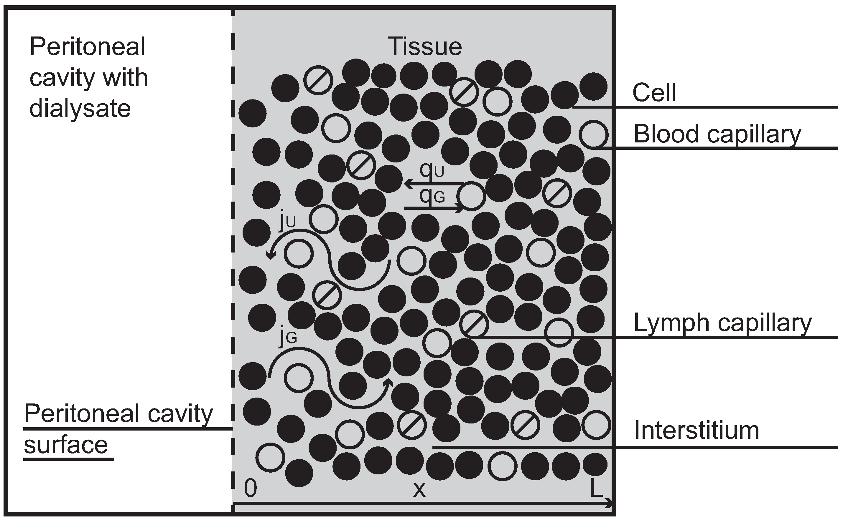
Peritoneal dialysis is a life saving treatment for chronic patients with end stage renal disease [1]. The peritoneal cavity, an empty space that separates bowels, abdominal muscles and other organs in the abdominal cavity, is applied as a container for dialysis fluid, which is infused there through a permanent catheter and left in the cavity for a few hours. During this time small metabolites (urea, creatinine) and large molecules (e.g., albumin) diffuse from blood that perfuses the tissue layers close to the peritoneal cavity to the dialysis fluid, and finally are removed together with the drained fluid. The treatment cycle (infusion, dwell, drainage) is repeated several times every day. The peritoneal transport occurs between dialysis fluid in the peritoneal cavity and blood passing down the capillaries in the tissue surrounding the peritoneal cavity (see Figure 1, in which a symmetrical structure of the tissue with respect to the cavity is assumed). Typically, many solutes are transported from blood to dialyzate, but some solutes such as for example an osmotic agent (glucose), which is present in a high concentration in dialysis fluid, are transported in the opposite direction, i.e., to the blood.

To the best of our knowledge, the first mathematical models for solute and fluid transport during peritoneal dialysis were proposed in the 1980s [2,3,4]. However, a rigorous mathematical description of fluid and solute transport between blood and dialysis fluid in the peritoneal cavity is still not formulated fully yet (in spite of the well-known basic physical laws for such transport) because of the complexity of the peritoneal transport. Recent mathematical and numerical studies introduced new concepts on peritoneal transport and yielded a better description of particular processes such as pure water transport, combined osmotic fluid flow and small solute transport, or water and proteins transport [5,6,7,8,9,10].

In [11], a new mathematical model for fluid and solute transport in peritoneal dialysis was constructed, which addresses the problem of a combined description of ultrafiltration to the peritoneal cavity, absorption of the osmotic agent (glucose) from the peritoneal cavity and the leakage of macromolecules (albumin) from the blood to the peritoneal cavity. The model is based on a three-component nonlinear system of two-dimensional partial differential equations for fluid, glucose and albumin transport with the relevant boundary and initial conditions. Under some assumptions the model was simplified in order to obtain exact formulae for spatially non-uniform steady-state solutions. As the result, the exact formulae for the fluid fluxes from blood to the tissue and across the tissue are constructed. It should be stressed that the analytical results presented in [11] were derived for the simplest profiles of the fractional fluid void volume ν (i.e., the volume occupied by the fluid in the interstitium while the rest of the tissue being cells and macromolecules is not allowed for fluid transport), namely ν is either a constant or a linear function with respect to the space variable x.

Here we go essentially further. Because experimental data (see, e.g., [12]) show that the fractional fluid void volume depends on the hydrostatic pressure in a nonlinear way, one should assume nonlinear profiles for ν. Moreover, the transportation of macromolecules (albumin is a typical example) essentially differs from the water and glucose transportation because of their large size. Usually it is taken into account by introducing a constant coefficient α in order to show that only a part of the fractional fluid void volume is accessible for such macromolecules. To avoid such a simplification, we introduce so-called fractional albumin volume ${\nu }_A$, which (like ν) depends on the hydrostatic pressure; however, it is not assumed that ${\nu }_A=\alpha \nu$, as in previous studies [9,11].

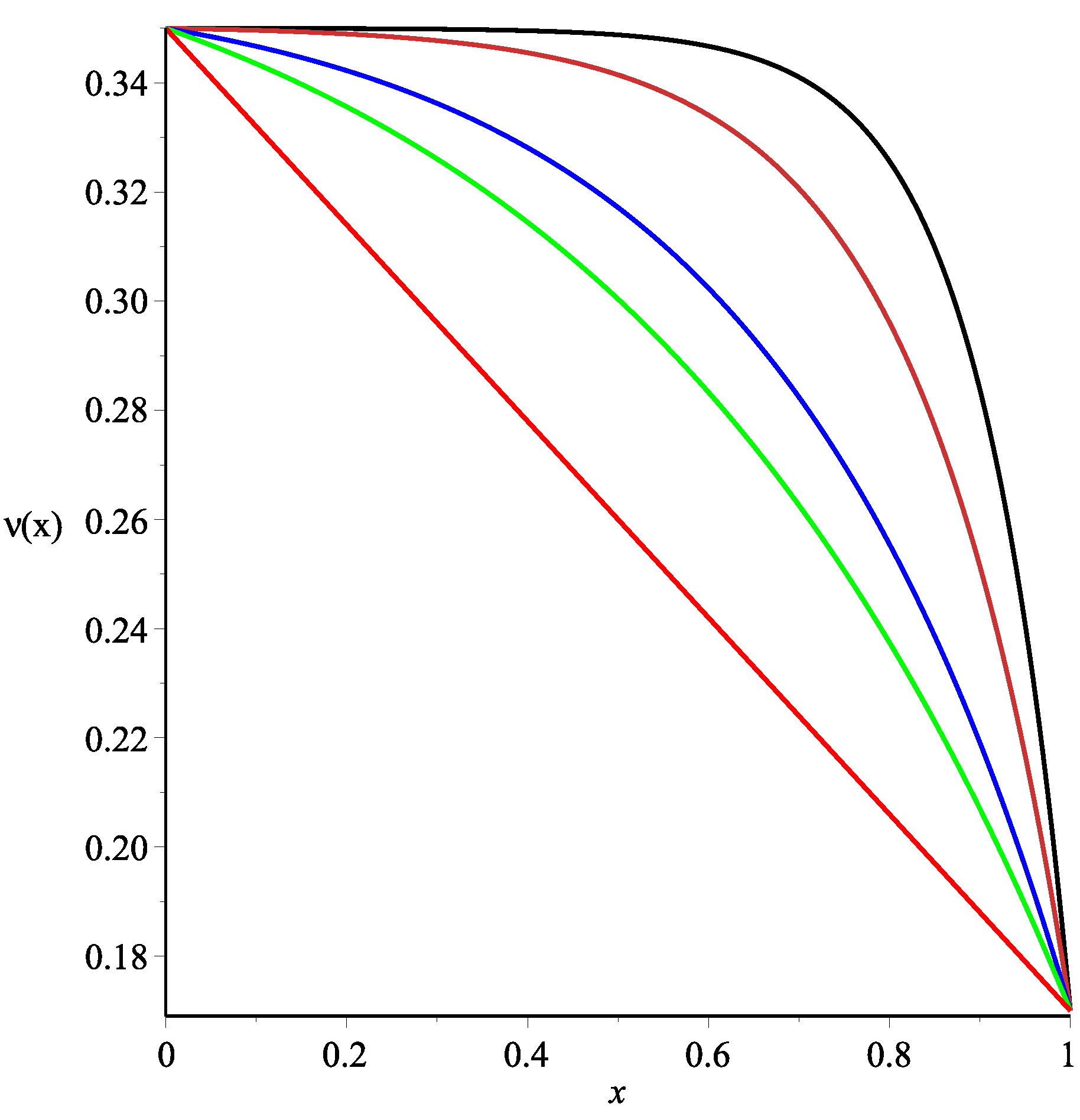
In order to obtain some analytical formulae, we used some correctly-specified profiles ${\nu }_A$ and ν, taking into account that both functions should be convex upwards along the main part of tissue (or at least in a vicinity of the point $x=0$ where the most intensive transport occurs, see Figure 2). Thus, exponential profiles for these functions were used because they are much closer to the profiles arising in experimental data than those studied in [11]. Under the same assumptions as in [11], new exact formulae (involving hypergeometric functions) for the fluid fluxes from blood to the tissue and across the tissue are constructed.

Analytical results are supplemented by numerical simulations for finding the albumin concentration and the albumin clearance for the real experimental data. As a result, we have shown that the albumin concentration within the tissue essentially depends on the function representing the fractional albumin volume ${\nu }_A$.

The obtained analytical results are compared to those obtained in [11] and checked for their applicability for the description of transport during peritoneal dialysis. In particular, using numerical simulations we established how the exact solutions found under pure mathematical assumptions differ from numerical ones obtained without any additional assumptions. As a result, it is shown that the analytical formulae obtained can describe the fluid and solute transport (especially the rate of ultrafiltration) for a wide range of values of parameters arising in the model.

The paper is organized as follows. In Section 2, an extended mathematical model of glucose and albumin transport in peritoneal dialysis is presented. In Section 3, new non-uniform steady-state solutions of the model are constructed and their properties are investigated. In Section 4, these solutions are tested for the real parameters that were taken from the references devoted to clinical treatments of peritoneal dialysis. The results are compared to those derived via analytical formulae in [11] and with numerical simulations obtained in [5,9,10]. Finally, we present some conclusions in the last section.

2. Mathematical Model

Here we present an extended version of the model of fluid and solute transport in peritoneal dialysis derived previously in [11]. The model was developed in one spatial dimension with $x=0$ representing the boundary of the peritoneal cavity and $x=L$ representing the end of the tissue surrounding the peritoneal cavity (see Figure 1). The model assumes the symmetrical structure of the surrounding tissue with respect to the cavity and the homogenous spreading of the source within the whole tissue as an approximation to the discrete structure of blood and lymphatic capillaries. The model also assumes that solutes are transported only within the interstitial fluid. Here we extend the model in order to take into account the possible dependence of several parameters on the hydrostatic pressure.

The mathematical description of transport processes within the tissue is based on the conservation law expressing a local balance of fluid volume and solute mass. For incompressible fluid, the change of volume may occur only due to the elasticity of the tissue. The fractional fluid void volume, i.e., the volume occupied by the fluid in the interstitium expressed per unit volume of the whole tissue, is denoted by $\nu (t,x)$, and its time evolution is described as:

$$\frac{\partial \nu }{\partial t}=-\frac{\partial j_U}{\partial x}+q_U-q_l$$

(1)

where $j_U(t,x)$ is the volumetric fluid flux across the tissue (ultrafiltration), $q_U(t,x)$ is the density of volumetric fluid flux from blood capillaries to the tissue, and $q_l>0$ is a known function, which depends on the hydrostatic pressure $P(t,x)$ and is the density of volumetric fluid flux from the tissue to the lymphatic vessels. Typically the function $q_l\left(P\right)$ is assumed to be linear [9] or a positive constant [11].

The equation that describes the local changes of glucose amount in the tissue, $\nu C_G$, is:

$$\frac{\partial \left(\nu C_G\right)}{\partial t}=-\frac{\partial j_G}{\partial x}+q_G,$$

(2)

where $C_G(t,x)$ is the glucose concentration in the tissue, $j_G(t,x)$ is the glucose flux through the tissue, and $q_G(t,x)$ is the density of the glucose flux from blood.

The equation that describes the local changes of albumin amount in the tissue, ${\nu }_A{C}_A$, has the form:

$$\frac{\partial \left({\nu }_A{C}_A\right)}{\partial t}=-\frac{\partial j_A}{\partial x}+q_A,$$

(3)

where $C_A(t,x)$, $j_A(t,x)$ and $q_A(t,x)$ correspond to the albumin concentration, albumin flux through the tissue and albumin flux from blood, respectively. Here the function ${\nu }_A(t,x)$ is introduced, which is called the fractional albumin volume. The function ${\nu }_A$ takes into account an obvious fact that only a part of the fractional fluid void volume ν is accessible for albumin because its molecular size is much larger than the glucose molecular size [7,9], so that ${\nu }_A<\nu$ for $\forall (t,x)\in {\mathbb{R}}^{+}\times (0,L)$. Usually it is assumed that ${\nu }_A=\alpha \nu$ ($\alpha <1$). However, we believe that it is an essential simplification. In fact, by introducing the coefficient $\alpha <1$, one simply assumes that, having any minimal $\nu ={\nu }_{min}$, a part of tissue is still accessible for such macromolecules. However, it is obvious that there exists a critical value of ν, for which only glucose and small metabolites are transported within tissue, while large molecules are completely blocked, i.e., $\alpha \approx 0$. On the other hand, $\alpha \approx 1$ provided the fractional void volume is sufficiently large, i.e., $\nu \approx {\nu }_{max}$. Thus, we replace $\alpha \nu$ by the function ${\nu }_A$.

In order to specify the fluxes arising in Equations (1)–(3), we assume that the osmotic pressure of glucose and the oncotic (this terminology is often used instead of “osmotic” for large proteins) pressure of albumin are described by the van’t Hoff law. Thus, the volumetric fluid flux across the tissue is generated by hydrostatic, osmotic and oncotic pressure gradients:

$$j_U=-\nu K\frac{\partial P}{\partial x}+{\sigma }_{TG}\nu KRT\frac{\partial C_G}{\partial x}+{\sigma }_{TA}\nu KRT\frac{\partial C_A}{\partial x},$$

(4)

where K is the hydraulic conductivity of the tissue that is assumed constant for simplicity(K may also depend on the pressure P), R is the gas constant, T is absolute temperature, and ${\sigma }_{TG}$ and ${\sigma }_{TA}$ are the Staverman reflection coefficients for glucose and albumin in the tissue, respectively. The density of fluid flux from blood to the tissue is generated, according to the Starling law, by the hydrostatic, osmotic and oncotic pressure differences between blood and tissue:

$$q_U=L_{p}a(P_B-P)-L_{p}a{\sigma }_{G}RT(C_{GB}-C_G)-L_{p}a{\sigma }_{A}RT(C_{AB}-C_A),$$

(5)

where $P(t,x)$ is the hydrostatic pressure, $L_{p}a$ is the hydraulic conductance of the capillary wall, $P_B$ is the hydrostatic pressure of blood, $C_{GB}$ and $C_{AB}$ are the glucose and albumin concentrations in blood, and ${\sigma }_G$ and ${\sigma }_A$ are the Staverman reflection coefficients for glucose and albumin in the capillary wall, respectively.

The glucose flux across the tissue is composed of a diffusive component (proportional to the glucose concentration gradient) and a convective component (proportional to glucose concentration and fluid flux):

$$j_G=-\nu D_G\frac{\partial C_G}{\partial x}+S_{TG}{C}_G{j}_U.$$

(6)

where $D_G$ is the diffusivity of glucose in the tissue, $S_{TG}=1-{\sigma }_{TG}$ is the sieving coefficients of glucose in the tissue [13].

The density of glucose flux between blood and the tissue consists of three components, namely a diffusive component (proportional to the difference of the glucose concentration in blood, $C_{GB}$, and the glucose concentration in the tissue, $C_G$), a convective component (proportional to the density of fluid flow from the blood to the tissue, $q_U$) and a component that represents lymphatic absorption of solutes (proportional to the density of volumetric lymph flux, $q_l$):

$$q_G=p_{G}a(C_{GB}-C_G)+S_G{q}_U{C}_G-q_l{C}_G.$$

(7)

where $p_{G}a$ is the diffusive permeability of the capillary wall for glucose and $S_G=1-{\sigma }_G$ is the sieving coefficients of glucose in the capillary wall.

In a similar way, the albumin flux across the tissue, $j_A(t,x)$, and the density of albumin flux to the tissue, $q_A(t,x)$, can be described as:

$$j_A=-{\nu }_A{D}_A\frac{\partial C_A}{\partial x}+S_{TA}{C}_A{j}_U,$$

(8)

$$q_A=p_{A}a(C_{AB}-C_A)+S_A{q}_U{C}_A-q_l{C}_A,$$

(9)

where $S_{TA}=1-{\sigma }_{TA}$ and $S_A=1-{\sigma }_A$ are the sieving coefficient of albumin in the tissue and in the capillary wall, respectively, $D_A$ is the diffusivity of albumin in the tissue, and $p_{A}a$ is the diffusive permeability of the capillary wall for albumin.

Equations (1)–(3) together with Equations (4)–(9) for flows form a system of three nonlinear second-order partial differential equations with five variables: $\nu ,{\nu }_A,P,C_G$ and $C_A$. Therefore, two additional equations are needed in order to construct a well defined model. Using data from experimental studies (see for the details [8]), we can obtain a constitutive equation describing how the fractional fluid void volume ν depends on interstitial pressure, P. In the general case, this equation has the form:

$$\nu =F\left(P\right),$$

(10)

where F is a monotonically non-decreasing bounded function with the limits: $F\to {\nu }_{min}$ if $P\to P_{min}$ and $F\to {\nu }_{max}$ if $P\to P_{max}$ (particularly, one may take $P_{min}=-\infty ,P_{max}=\infty$). Here ${\nu }_{min}<{\nu }_{max}$ and ${\nu }_{max}<1$ are empirically measured constants. In the case of the fractional void volume for albumin ${\nu }_A$, we propose to use the similar formulae:

$${\nu }_A=F_A\left(P\right),$$

(11)

where $F_A$ is another monotonically non-decreasing bounded function with the limits: $F_A\to {\nu }_{Amin}$ if $P\to P_{min}$ and $F_A\to {\nu }_{Amax}$ if $P\to P_{max}$. Obviously ${\nu }_{Amin}\le {\nu }_{min}$ and ${\nu }_{Amax}\le {\nu }_{max}$.

Finally, boundary and initial conditions can be defined as follows. Since experimental data and theoretical studies suggest that intraperitoneal pressure $P_D$, glucose $C_{GD}$ and albumin $C_{AD}$ concentrations in the peritoneal cavity are constant for some time period (see for the details [8,9,10]), the constant Dirichlet conditions for the tissue layer in contact with the peritoneal cavity:

$$x=0:P=P_D,C_G=C_{GD},C_A=C_{AD}$$

(12)

can be taken. Boundary conditions on another boundary of the tissue layer of the width L are the zero flux conditions

$$x=L:\frac{\partial P}{\partial x}=0,\frac{\partial C_G}{\partial x}=0,\frac{\partial C_A}{\partial x}=0.$$

(13)

i.e., the tissue is impermeable at $x=L$.

The initial conditions describe equilibrium within the tissue without any contact with dialysis fluid:

$$t=0:P=P^{*},C_G=C_G^{*},C_A=C_A^{*},$$

(14)

where $P^{*},C_G^{*},$ and $C_A^{*}$ are some non-negative values, which have been specified in [11].

Note that Equations (1)–(11) can be: united into three nonlinear partial differential equations (PDEs) for hydrostatic pressure $P(t,x)$, glucose concentration $C_G(t,x)$ and albumin concentration $C_A(t,x)$. Thus, these three PDEs together with boundary and initial Conditions (12)–(14) form a nonlinear boundary-value problem.

3. Non-Uniform Steady-State Solutions of the Model

The time needed to approach the steady state is of the order of minutes for small solutes, such as glucose. One increases for much larger solutes, especially for albumin. However, if we take into account that patients are on continuously repeated treatment and that there are a few exchanges of dialysis fluid per day, the transport system for large molecules after many exchanges is also close to the steady state (see more detailed discussion e.g., in [14]). Thus, the solutions for the steady state of the system should be considered as good approximations for real conditions in the tissue in this clinical setting.

Firstly, we note that there is a special steady state of the tissue in its physiological state without dialysis, and, therefore, no transport to the peritoneal cavity occurs. In this case, the boundary conditions at $x=0$ given by Equation (12) are replaced by zero Neumann conditions, and the steady-state solution can be easily found by solving the equations

$$q_U-q_l=0,q_G=0,q_A=0.$$

(15)

This is a system of algebraic equations and in order to solve one, we only need to specify the function $q_l\left(P\right)$. In the general case, one obtains the spatially uniform steady-state concentrations of glucose and albumin in the form:

$$\begin{array}{c}{C}_G^{*}=\frac{p_{G}a}{p_{G}a+{\sigma }_G{q}_l\left(P\right)}{C}_{GB},\hfill \\ C_A^{*}=\frac{p_{A}a}{p_{A}a+{\sigma }_A{q}_l\left(P\right)}{C}_{AB},\hfill \end{array}$$

(16)

where the hydrostatic pressure is a solution of the transcendent equation:

$$P-P_B+\frac{1}{L_{p}a}{q}_l\left(P\right)=RT\left(\frac{{\sigma }_G^2{q}_l\left(P\right)}{p_{G}a+{\sigma }_G{q}_l\left(P\right)}+\frac{{\sigma }_A^2{q}_l\left(P\right)}{p_{A}a+{\sigma }_A{q}_l\left(P\right)}\right).$$

(17)

The equation can be explicitly solved for the simplest functions $q_l\left(P\right)$ only. For example, a cubic equation is obtained in the case of the linear function $q_l=q_{l0}+q_{l0}P$; hence their roots can be derived. Notably, setting $q_l=0$, Equations (16)–(17) produce the constant steady-state

$$C_G^{*}=C_{GB},C_A^{*}=C_{AB},P^{*}=P_B,$$

(18)

which one expects to get without any mathematical modeling.

However, a constant steady-state solution cannot describe fluid and solute transport in peritoneal dialysis. Having in mind constructing non-uniform steady-state solutions, we transform the nonlinear boundary-value problem presented above to an equivalent form by introducing non-dimensional independent and dependent variables (except for ν and ${\nu }_A$, those are non-dimensional variables) of the form

$$x^{*}=\frac{x}{L},t^{*}=\frac{K{P}_{D}t}{L^2},$$

(19)

$$p(t^{*},x^{*})=\frac{P}{P_D},u(t^{*},x^{*})=\frac{C_G-C_{GB}}{C_{GD}-G_{GB}},w(t^{*},x^{*})=\frac{C_A}{C_{GD}-G_{GB}}.$$

(20)

Thus, after rather simple calculations and taking into account Equations (4), (6) and (8), one obtains Equations (1)–(3) in the form (hereafter upper index * is omitted):

$$\begin{array}{c}c\frac{\partial \nu }{\partial t}=\frac{\partial }{\partial x}\left(\frac{\nu \partial p}{\partial x}\right)-t_0{\sigma }_1\frac{\partial }{\partial x}\left(\frac{\nu \partial u}{\partial x}\right)-t_0{\sigma }_2\frac{\partial }{\partial x}\left(\frac{\nu \partial w}{\partial x}\right)+t_0(q_U-q_l),\end{array}$$

(21)

$$\begin{array}{c}\frac{\partial \left(\nu u\right)}{\partial t}+{\sigma }_{TG}{u}_0\frac{\partial \nu }{\partial t}=d_1{t}_0\frac{\partial }{\partial x}\left(\frac{\nu \partial u}{\partial x}\right)+S_{TG}\frac{\partial }{\partial x}\left(\frac{u\nu \partial p}{\partial x}\right)\hfill \\ -S_{TG}{t}_0{\sigma }_1\frac{\partial }{\partial x}\left(\frac{u\nu \partial u}{\partial x}\right)-S_{TG}{t}_0{\sigma }_2\frac{\partial }{\partial x}\left(\frac{u\nu \partial w}{\partial x}\right)\hfill \\ +t_0(S_{G}u+u_0(S_G-S_{TG}))q_U-t_0{b}_{1}u-t_0{\sigma }_{TG}{u}_0{q}_l,\hfill \end{array}$$

(22)

$$\begin{array}{c}\frac{\partial \left({\nu }_{A}w\right)}{\partial t}=d_2{t}_0\frac{\partial }{\partial x}\left(\frac{{\nu }_A\partial w}{\partial x}\right)+S_{TA}\frac{\partial }{\partial x}\left(\frac{w\nu \partial p}{\partial x}\right)\hfill \\ -S_{TA}{t}_0{\sigma }_1\frac{\partial }{\partial x}\left(\frac{w\nu \partial u}{\partial x}\right)-S_{TA}{t}_0{\sigma }_2\frac{\partial }{\partial x}\left(\frac{w\nu \partial w}{\partial x}\right)\hfill \\ +t_0{S}_{A}w{q}_U-t_0{b}_{2}w-t_0{w}_0(b_2-q_l),\hfill \end{array}$$

(23)

where

$$\begin{array}{c}{q}_U=\beta \left(\frac{1}{t_0}(p_0-p)+\frac{{\sigma }_G{\sigma }_1}{{\sigma }_{TG}}u+\frac{{\sigma }_A{\sigma }_2}{{\sigma }_{TA}}(w-w_0)\right),\beta =\frac{L_{p}a{L}^2}{K},\hfill \\ {\sigma }_1={\sigma }_{TG}KRT\frac{C_{GD}-G_{GB}}{L^2},{\sigma }_2={\sigma }_{TA}KRT\frac{C_{GD}-G_{GB}}{L^2},\hfill \\ d_1=\frac{D_G}{L^2},d_2=\frac{D_A}{L^2},\hfill \\ b_1=p_{G}a+q_l,b_2=p_{A}a+q_l,\hfill \\ u_0=\frac{C_{GB}}{C_{GD}-G_{GB}},w_0=\frac{C_{AB}}{C_{GD}-G_{GB}},p_0=\frac{P_B}{P_D}\hfill \\ t_0=\frac{L^2}{K{P}_D},w^{*}=w-w_0,\hfill \end{array}$$

(24)

Now we want to find the steady-state solutions of Equations (21)–(23) satisfying the boundary Conditions (12)–(13). They take the form:

$$x=0:p=1,u=1,w=\frac{C_{AD}}{C_{GD}-G_{GB}}$$

(25)

$$x=1:\frac{\partial p}{\partial x}=0,\frac{\partial u}{\partial x}=0,\frac{\partial w}{\partial x}=0.$$

(26)

for the non-dimensional variables. In order to find the steady-state solutions, Equations (21)–(23) should be reduced to the system of ordinary differential equations (ODEs):

$$\frac{1}{t_0}\frac{d}{dx}\left(\frac{\nu dp}{dx}\right)-{\sigma }_1\frac{d}{dx}\left(\frac{\nu du}{dx}\right)-{\sigma }_2\frac{d}{dx}\left(\frac{\nu dw}{dx}\right)+q_U-q_l=0,$$

(27)

$$\begin{array}{cc}& d_1\frac{d}{dx}\left(\frac{\nu du}{dx}\right)+\frac{S_{TG}}{t_0}\frac{d}{dx}\left(\frac{u\nu dp}{dx}\right)-S_{TG}{\sigma }_1\frac{d}{dx}\left(\frac{u\nu du}{dx}\right)\hfill \\ & -S_{TG}{\sigma }_2\frac{d}{dx}\left(\frac{u\nu dw}{dx}\right)+(S_{G}u+u_0(S_G-S_{TG}))q_U-b_{1}u-{\sigma }_{TG}{u}_0{q}_l=0,\hfill \end{array}$$

(28)

$$\begin{array}{cc}& d_2\frac{d}{dx}\left(\frac{{\nu }_{A}dw}{dx}\right)+\frac{S_{TA}}{t_0}\frac{d}{dx}\left(\frac{(w-w_0)\nu dp}{dx}\right)-S_{TA}{\sigma }_1\frac{d}{dx}\left(\frac{(w-w_0)\nu du}{dx}\right)\hfill \\ & -S_{TA}{\sigma }_2\frac{d}{dx}\left(\frac{(w-w_0)\nu dw}{dx}\right)+(S_{A}w-S_{TA}{w}_0)q_U-b_2(w-w_0)-{\sigma }_{TA}{w}_0{q}_l=0.\hfill \end{array}$$

(29)

Unfortunately, the non-linear system of ODEs Equations (27)–(29) is still very complex and cannot be integrated in the case of arbitrary coefficients, i.e., it seems to be impossible to find non-uniform steady-state solutions. Thus, one may look for the correctly-specified coefficients, for which this system can be simplified. It was noted in [11] that the relations:

$$S_A=S_{TA},S_G=S_{TG}$$

(30)

lead to an essential (this means that automatically ${\sigma }_G={\sigma }_{TG},{\sigma }_A={\sigma }_{TA}$) simplification of this system. Using Assumption (30), one arrives at the semi-coupled system of ODEs:

$$\frac{1}{\beta }\frac{d}{dx}\left(\nu \frac{d{q}_U}{dx}\right)=q_U-q_l$$

(31)

$$j_U=\frac{L}{\beta }\frac{d{q}_U}{dx}$$

(32)

to find the functions $q_U$ and $j_U$ provided the functions ν and $q_l$ are known. Since the functions $q_U$ and $j_U$ are expressed via $p,u$ and w and its first-order derivatives, boundary Conditions (25)–(26) take the form:

$$x=0:q_U=\beta \left(\frac{1}{t_0}(p_0-1)+{\sigma }_1+{\sigma }_2\frac{C_{AD}-C_{AB}}{C_{GD}-G_{GB}}\right)$$

(33)

$$x=1:\frac{\partial q_U}{\partial x}=0,j_U=0.$$

(34)

However ν and $q_l$ depend on the pressure $p\left(x\right)$, which is also unknown function, and therefore we need to to use the function F from Formula (10). Since the function $F\left(p\right(x\left)\right)$ is decreasing (with respect to x!) provided $p\left(x\right)$ is a spatially non-uniform steady-state solution, the function $\nu \left(x\right)$ is also a decreasing function from $\nu \left(0\right)={\nu }_{max}$ till $\nu \left(1\right)={\nu }_{min}$. Therefore, fixing an appropriate function $\nu \left(x\right)$ and finding the function $q_l\left(p\right)=F^{-1}\left(\nu \left(x\right)\right)$ ($F^{-1}$ is an inverse function to F), one obtains ODE (31) in the form:

$$\frac{1}{\beta }\frac{d}{dx}\left(\nu \left(x\right)\frac{d{q}_U}{dx}\right)=q_U-F^{-1}\left(\nu \left(x\right)\right)$$

(35)

The simplest case occurs when $q_l=constant$ and the function is the linear function of the form

$$\nu \left(p\left(x\right)\right)\equiv \nu \left(x\right)={\nu }_{max}-({\nu }_{max}-{\nu }_{min})x,x\in [0,1].$$

(36)

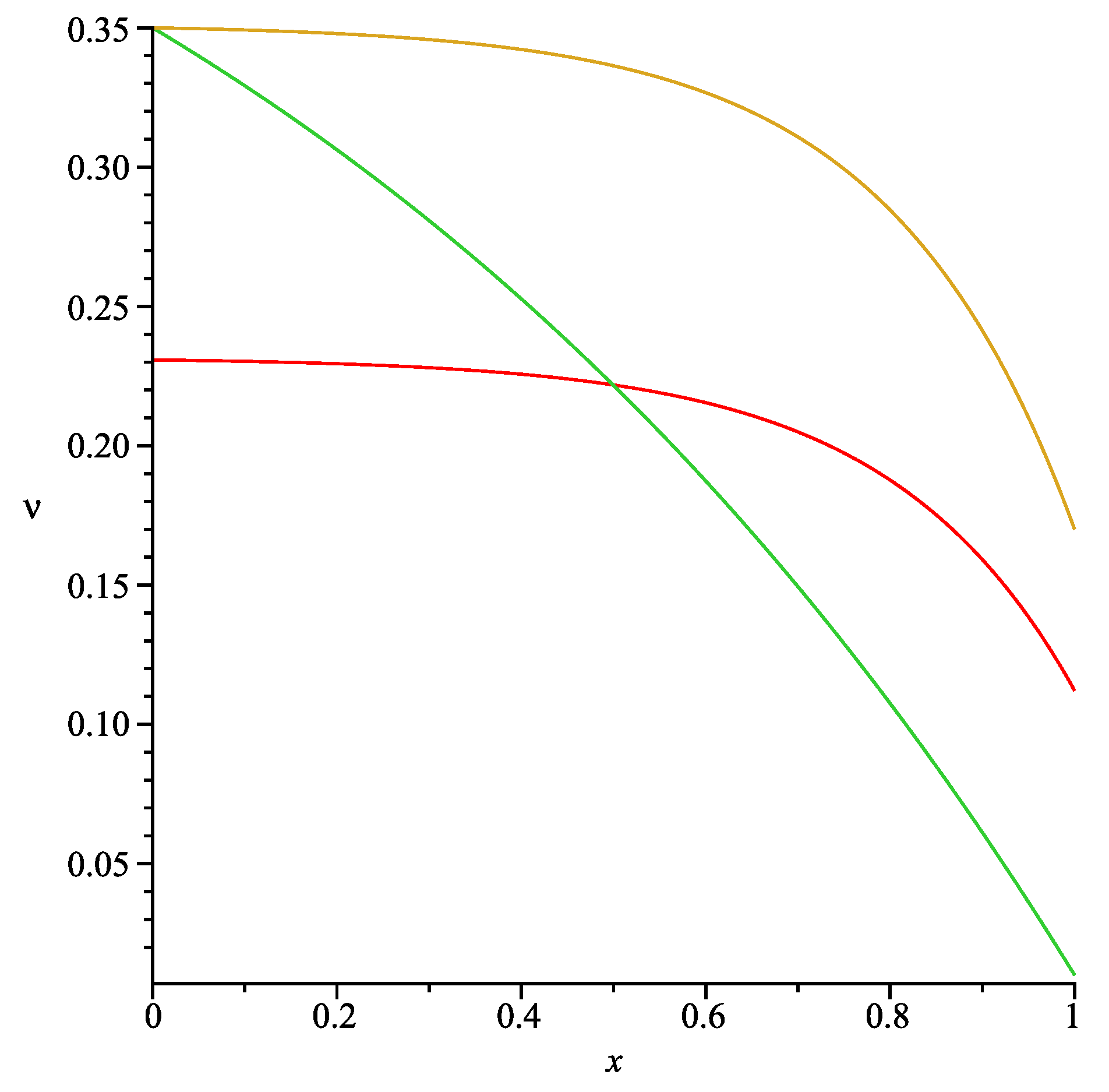
This case was examined in [11]. While the assumption about the constant density $q_l$ of flux from the tissue to the lymphatic vessels is quite reasonable, experimental data say that the function $\nu \left(x\right)$ describing the fractional fluid void volume is more complicated. In particular, this function should be convex upwards (at least in a vicinity of the point $x=0$). Here we consider exponential profiles for $\nu \left(x\right)$ of the form:

$$\nu \left(x\right)={\nu }_0-{\nu }_1{e}^{\alpha x}$$

(37)

where

$${\nu }_0=\frac{{\nu }_{max}{e}^{\alpha }-{\nu }_{min}}{e^{\alpha }-1},{\nu }_1=\frac{{\nu }_{max}-{\nu }_{min}}{e^{\alpha }-1}$$

in order to obtain ${\nu }_{min}$ and ${\nu }_{max}$ for $x=1$ and $x=0$ respectively. Obviously Formula (37) produces a wide range of profiles depending on values of the positive parameter α (see Figure 2).

Substituting (37) into (31), we obtain the linear second-order ODE with variable coefficients:

$$({\nu }_0-{\nu }_1{e}^{\alpha x})\frac{d^{2}q}{d{x}^2}-\alpha {\nu }_1{e}^{\alpha x}\frac{dq}{dx}-\beta q=0,$$

(38)

where $q=q_U-q_l$.

Here we obtain two forms of its solutions in explicit form. The first one can be expressed via elementary functions while the second involves hypergeometric functions.

Let us construct the first one, which can be derived for a specific value of the parameter α only. In fact, a particular solution of Equation (38) has been found in the form $q_{part}=e^{-\alpha x},$ provided α is the solution of the transcendental equation:

$${\alpha }^2\frac{{\nu }_{max}}{\beta }=\frac{e^{\alpha }-1}{e^{\alpha }-\frac{{\nu }_{min}}{{\nu }_{max}}}.$$

(39)

In particular, using the parameter values presented in

Table 1. Parameters of the model used for numerical analysis of peritoneal transport. The values of parameters are taken from (Waniewski et al. 2007; Stachowska-Pietka et al. 2007); Cherniha et al. 2014).

Parameter Name	Parameter Symbol, Value and Unit
Minimal fractional void volume	${\nu }_{min}=0.17$
Maximal fractional void volume	${\nu }_{max}=0.35$
Staverman reflection coefficient for glucose	${\sigma }_{TG}$ varies from 0 to $0.05$
Sieving coefficient of glucose in tissue	$S_{TG}=1-{\sigma }_{TG}$
Staverman reflection coefficient for albumin	${\sigma }_{TA}$ varies from $0.05$ to $0.5$
Sieving coefficient of albumin in tissue	$S_{TA}=1-{\sigma }_{TA}$
Hydraulic permeability of tissue	$K=5.14·{10}^{-5}$ $c{m}^2·mi{n}^{-1}·mmH{g}^{-1}$
Gas constant times temperature	$RT=18·{10}^3$ $mmHg·mmo{l}^{-1}·mL$
Width of tissue layer	$L=1.0$ $cm$
Hydraulic permeability of capillary wall	$L_{P}a=$
times density of capillary surface area	$7.3·{10}^{-5}$ $mi{n}^{-1}·mmH{g}^{-1}$
Volumetric fluid flux to lymphatic vessels	$q_l=0.26·{10}^{-4}$ $mi{n}^{-1}$
Diffusivity of glucose in tissue divided by ${\nu }_{min}$	$D_G=12.11·{10}^{-5}$ $c{m}^2·mi{n}^{-1}$
Diffusivity of albumin in tissue divided by ${\nu }_{min}$	$D_A=1.62·{10}^{-5}$ $c{m}^2·mi{n}^{-1}$
Permeability of capillary wall for glucose	$p_{G}a=$
times density of capillary surface area	$3.4·{10}^{-2}$ $mi{n}^{-1}$
Permeability of capillary wall for albumin	$p_{A}a=$
times density of capillary surface area	$6·{10}^{-5}$ $mi{n}^{-1}$
Glucose concentration in blood	$C_{GB}=6·{10}^{-3}$ $mmol·m{L}^{-1}$
Albumin concentration in blood	$C_{AB}=0.6·{10}^{-3}$ $mmol·m{L}^{-1}$
Glucose concentration in dialysate	$C_{GD}=180·{10}^{-3}$ $mmol·m{L}^{-1}$
Albumin concentration in dialysate	$C_{AD}=0$
Hydrostatic pressure of blood	$P_B=15$ $mmHg$
Hydrostatic pressure of dialysate	$P_D$ varies from 3 to 12 $mmHg$

(see Section 4), we have calculated that $\alpha \approx 1.93$. Using this particular solution, we obtain the general solution:

$$q_U=c_1{e}^{-\alpha x}+c_2({\nu }_0{e}^{-\alpha x}ln\left({\nu }_0-{\nu }_1{e}^{\alpha x})+{\nu }_1\right)+q_l.$$

(40)

via the well-known formula.

Substituting (40) into (32), the fluid flux:

$$j_U=-\frac{{\nu }_0-{\nu }_1{e}^{\alpha x}}{\beta }\left(c_1\alpha e^{-\alpha x}+c_2{\nu }_0\alpha \left(e^{-\alpha x}ln({\nu }_0-{\nu }_1{e}^{\alpha x})+\frac{{\nu }_1}{{\nu }_0-{\nu }_1{e}^{\alpha x}}\right)\right)$$

(41)

has been calculated. The constants $c_1$ and $c_2$ can be specified using the boundary Conditions (33)–(34), namely:

$$c_1=\kappa \frac{q_0-q_l}{\kappa +{\nu }_{0}ln({\nu }_o-{\nu }_1)+{\nu }_1},c_2=\frac{q_0-q_l}{\kappa +{\nu }_{0}ln({\nu }_o-{\nu }_1)+{\nu }_1},$$

(42)

where:

$$q_0=\beta \left(\frac{1}{t_0}(p_0-1)+{\sigma }_1+{\sigma }_2(1-w_0)\right),$$

$$\kappa =-{\nu }_{0}ln({\nu }_0-{\nu }_1{e}^{\alpha })-\frac{{\nu }_0{\nu }_1{e}^{\alpha }}{{\nu }_0-{\nu }_1{e}^{\alpha }}.$$

The exact solution of Equation (38) for an arbitrary value of the parameter α can be found as follows. The transformation (see e.g., [15]) $\xi =-{\nu }_1{e}^{\alpha x}$, $\omega =q{\xi }^{-k}$, where k is the root of the quadratic equation ${\nu }_0{\alpha }^2{k}^2-\beta =0$, leads to the equation:

$$\xi (\xi +{\nu }_0){\omega }_{\xi \xi }^{\prime \prime }+(2(k+1)\xi +{\nu }_0(2k+1))w_{\xi }^{\prime }+k(k+1)\omega =0.$$

(43)

The substitution $\xi =-{\nu }_{0}z$ leads to the hypergeometric equation:

$$z(z-1){\omega }_{zz}^{\prime \prime }+((2k+2)z-(2k+1)){\omega }_z^{\prime }+k(k+1)\omega =0.$$

(44)

It is well-known that the general solution of Equation (44) has the form:

$$\begin{array}{c}\hfill \omega =c_{1}F(k,k+1,2k+1;z)+c_2{z}^{-2k}F(-k,-k+1,-2k+1;z),\end{array}$$

(45)

where $F(·,·,·;·)$ is the hypergeometric function. Turning back to the original notations, we obtain the following formula for the density of fluid flux from blood to the tissue:

$$\begin{array}{cc}\hfill q_U& =c_1{e}^{k\alpha x}F\left(k,k+1,2k+1;\frac{{\nu }_1}{{\nu }_0}{e}^{\alpha x}\right)\hfill \\ & +c_2{e}^{-k\alpha x}F\left(-k,-k+1,-2k+1;\frac{{\nu }_1}{{\nu }_0}{e}^{\alpha x}\right)+q_l,\hfill \end{array}$$

(46)

where $k=\frac{1}{\alpha }\sqrt{\frac{L_{p}a{L}^2}{K{\nu }_0}}.$

Substituting (46) into (32) and using the known properties of hypergeometric functions (see e.g., [16]), the fluid flux of the form:

$$\begin{array}{cc}\hfill j_U& =\frac{K\nu }{L_{p}aL}\left(c_1\right(k\alpha e^{k\alpha x}F(k,k+1,2k+1;\frac{{\nu }_1}{{\nu }_0}{e}^{\alpha x})\hfill \\ & +\frac{{\nu }_1}{{\nu }_0}\frac{k(k+1)}{2k+1}\alpha e^{(k+1)\alpha x}F(k+1,k+2,2k+2;\frac{{\nu }_1}{{\nu }_0}{e}^{\alpha x}))\hfill \\ & +c_2(-k\alpha e^{-k\alpha x}F(-k,-k+1,-2k+1;\frac{{\nu }_1}{{\nu }_0}{e}^{\alpha x})\hfill \\ & +\frac{{\nu }_1}{{\nu }_0}\frac{-k(-k+1)}{-2k+1}\alpha e^{(-k+1)\alpha x}F(-k+1,-k+2,-2k+2;\frac{{\nu }_1}{{\nu }_0}{e}^{\alpha x})\left)\right)\hfill \end{array}$$

(47)

is obtained. Hereafter, the following notations are used:

$$\begin{array}{cc}& f_1=F(k,k+1,2k+1;\frac{{\nu }_1}{{\nu }_0})\hfill \\ & f_2=F(-k,-k+1,-2k+1;\frac{{\nu }_1}{{\nu }_0})\hfill \\ & f_3=F(k,k+1,2k+1;\frac{{\nu }_1}{{\nu }_0}{e}^{\alpha })\hfill \end{array}\begin{array}{cc}& f_4=F(k+1,k+2,2k+2;\frac{{\nu }_1}{{\nu }_0}{e}^{\alpha })\hfill \\ & f_5=F(-k,-k+1,-2k+1;\frac{{\nu }_1}{{\nu }_0}{e}^{\alpha })\hfill \\ & f_6=F(-k+1,-k+2,-2k+2;\frac{{\nu }_1}{{\nu }_0}{e}^{\alpha })\hfill \end{array}$$

(48)

$$\begin{array}{cc}& h_1=k\alpha e^{-k\alpha x}{f}_3+\frac{{\nu }_1}{{\nu }_0}\frac{k(-k+1)}{-2k+1}\alpha e^{(-k+1)\alpha }{f}_4\hfill \\ & h_2=k\alpha e^{k\alpha x}{f}_5+\frac{{\nu }_1}{{\nu }_0}\frac{k(k+1)}{2k+1}\alpha e^{(k+1)\alpha }{f}_6\hfill \end{array}$$

(49)

Unknown constants $c_1$ and $c_2$ can be specified using the boundary Conditions (33)–(34); hence the formulae:

$$c_1=\frac{h_1(q_0-q_l)}{h_1{f}_1+h_2{f}_2},c_2=\frac{h_2(q_0-q_l)}{h_1{f}_1+h_2{f}_2}$$

(50)

were obtained.

Thus, we have found the formulae for $q_U$ and $j_U$, which present the exact solution of ODEs (26) and (32) and the boundary Conditions (33)–(34). In other words, the exact formulae for non-uniform steady-state solutions describing the fluid flux across the tissue, $j_U$, and the fluid flux from blood to the tissue, $q_U$, during peritoneal dialysis are constructed.

Having these formulae, the concentrations of glucose and albumin in the tissue can be found by solving linear second-order ODEs:

$$d_1\frac{d}{dx}\left(({\nu }_0-{\nu }_1{e}^{\alpha x})\frac{du}{dx}\right)-\frac{S_G}{L}{j}_U\left(x\right)\frac{du}{dx}-(p_{G}a+{\sigma }_G{q}_l)u-{\sigma }_G{u}_0{q}_l=0,$$

(51)

$$d_2\frac{d}{dx}\left({\nu }_A\left(x\right)\frac{dw}{dx}\right)-\frac{S_A}{L}{j}_U\left(x\right)\frac{dw}{dx}-(p_{A}a+{\sigma }_A{q}_l)w+p_{A}a{w}_0=0,$$

(52)

taking into account the boundary Conditions (25)–(26). Here the function ${\nu }_A$ should be prescribed according to (11) (see Section 5 for details); the functions $q_U$ and $j_U$ are defined by Formula (40) and (41). Note that Equations (51)–(52) can be easily constructed using ODEs (28)–(29), restrictions (30) and relations (31)–(32), i.e., these ODEs have the same structure for arbitrary given functions $q_U$ and $j_U$.

Finally, hydrostatic pressure $p\left(x\right)$ is easily obtained provided the glucose concentration $u\left(x\right)$ and the albumin concentration $w\left(x\right)$ are known using the first Formula in (24).

4. Numerical Results and Their Application for Peritoneal Dialysis without the Albumin Transport

Here we present numerical results based on the formulae derived in Section 3. Our aims are to compare the results with those obtained earlier and to check whether they are applicable for describing the fluid-glucose-albumin transport in peritoneal dialysis. The parameters used in the formulae were mostly taken from [11] and are presented in Table 1.

In order to compare the numerical results obtained here with those for osmotic peritoneal transport derived earlier, in which albumin transport was not considered, we neglect the oncotic pressure as a driving fluid force across the tissue, i.e., we put the Staverman reflection coefficients for albumin ${\sigma }_{TA}={\sigma }_A=0$. This means that the fluid flux across the tissue, $j_U$, and the fluid flux from blood to the tissue, $q_U$ (see Formulae (4) and (5)), do not depend on the albumin concentration, i.e., $C_A=C_{AB}=0$. Especially we pay attention to the fluid flux $j_U(t,0)$ (ultrafiltration flow ), which describes the net exchange of fluid between the tissue and the peritoneal cavity across the peritoneal surface and therefore shows the efficiency of removal of water during peritoneal dialysis. The assessment of ultrafiltration flow is very important from a practical point of view because low values of this flow in some patients indicate that some problems with osmotic fluid removal have occurred, which may finally result in the failure of the therapy [17]. Note that the ultrafiltration flow values calculated below under restrictions ${\sigma }_{TA}=0$ will be larger than without this restriction (the sign of the last term in (4) is opposite to the previous one because oncotic and osmotic pressures act in the opposite directions).

Because of the unsolved problem of the values for Staverman reflection coefficients, which cannot be directly measured (see [18] for details), we concentrated on the coefficient ${\sigma }_G$, namely to establish how peritoneal transport depends on values of ${\sigma }_G$. All of the other parameters were fixed and are listed in Table 1. However, taking into account that the hydrostatic pressure of dialyzate $P_D$ may essentially vary (depending on individual characteristics of patients), we have done also numerical simulations in order to estimate the impact of this parameter.

Having the function $q_U$ and the function $j_U$, the concentration of glucose u in the tissue can be found by numerically solving the linear ODE (51) , finally the hydrostatic pressure p is obtained using the first formula in (24).

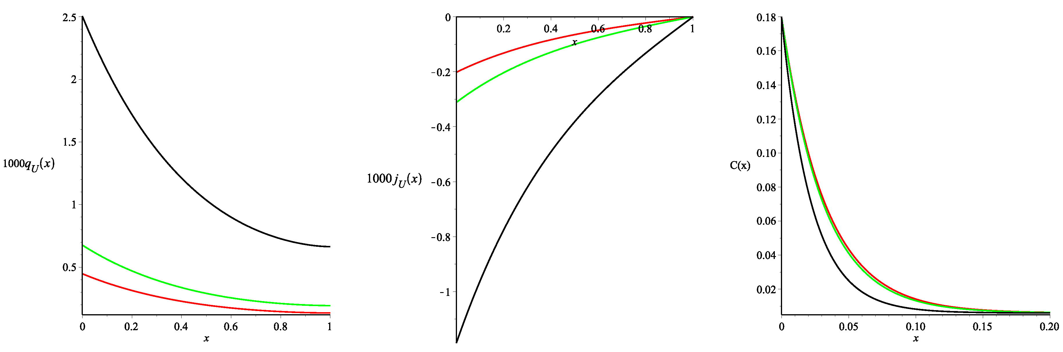
The results are presented in Figure 3 (all of the curves presented in the paper were constructed using the package Maple 17). As one may note three different values of the Staverman reflection coefficient ${\sigma }_G$ were used. Figure 3 presents the spatial distributions of the steady-state density of the fluid flux from blood to the tissue $q_U$ and the fluid flux across the tissue $j_U$, calculated using Formulae (46)–(50). Negative values of $j_U$ indicate that the net fluid flux occurs across the tissue towards the peritoneal cavity. Therefore it corresponds to the water removal by ultrafiltration. The monotonically decreasing (with the distance from the peritoneal surface) function $q_U\left(x\right)$ and the monotonically increasing function $j_U\left(x\right)$ are in agreement with the experimental data and previously obtained numerical results for the models that took into account only the glucose transport (see for the details [5,10] and the references cited therein).

Moreover, we noted that the values of the fluxes $q_U$ and $j_U$ obtained here slightly differ from those obtained in [11] for the same parameters and the linear profile (36). In particular, using the value of the fluid flux $j_U$ at the point $x=0$, one may calculate the ultrafiltration flow. Total fluid outflow from the tissue to the cavity (ultrafiltration), calculated assuming that the surface area of the contact between dialysis fluid and peritoneum is equal to $5\times {10}^3$ cm${}^2$ (a typical value for this surface [19]), is $1.0$, $1.6$ and $6.0$ mL/min for the the Staverman reflection coefficients $0.001$, $0.002$ and $0.01$, respectively. Thus, the ultrafiltration is about $5\%$ higher than the one obtained in [11]. Obviously, this difference is a consequence of the profile change for the fractional void volume (see Figure 2).

Figure 3 also presents the spatial distributions of the glucose concentration in the tissue (see the right picture) depending on the values of ${\sigma }_{TG}$. The interstitial glucose concentration $C_G$ decreases rapidly with the distance from the peritoneal surface to the constant steady-state value of $C_G^{*}$ (see Formula (15) in [11]) independently of the ${\sigma }_{TG}$ values. This remains in agreement with the previous results obtained in [5,11].

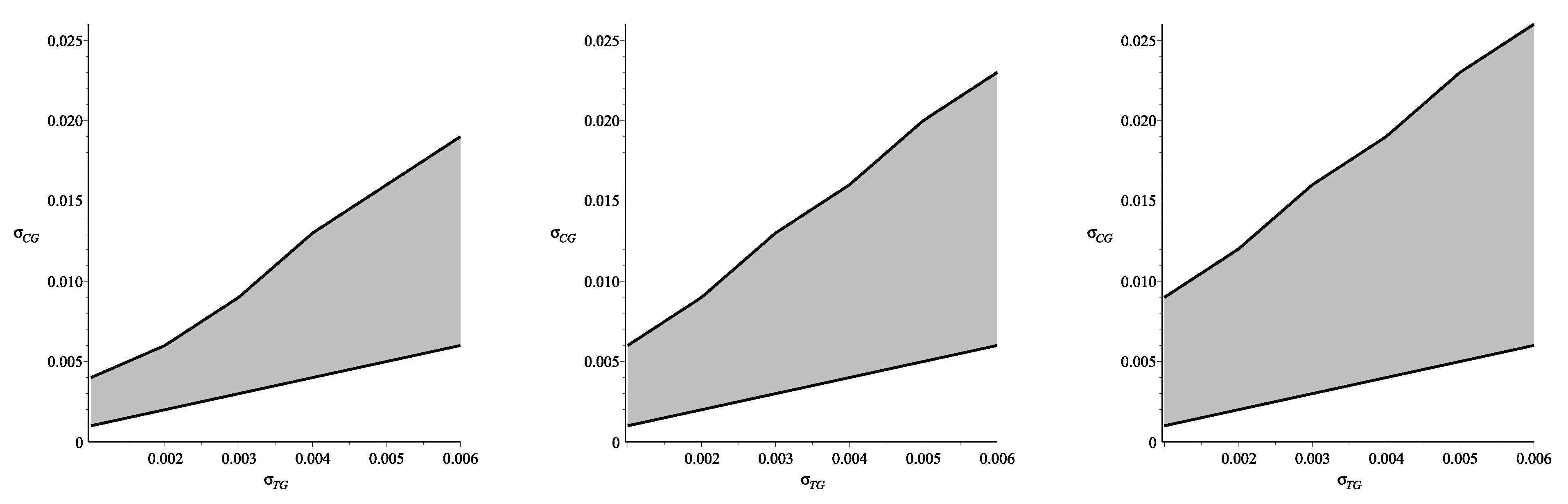
Because the assumption about the equality of the reflection coefficients in the tissue and in the capillary wall, which demonstrates an interesting specific symmetry in the equations, can be too restrictive for practical applications of the derived formulae, one needs to provide some additional justification. As it follows from the biophysical interpretation of these coefficients, the inequality ${\sigma }_{TG}<{\sigma }_{CG}$ takes place instead of (30). Having this in mind, we have done numerical simulations in order to define a domain, in which the formulae obtained can be applied for the calculation of ultrafiltration during peritoneal dialysis. In order to define this domain we have calculated $q_U$ and $j_U$ using the values of parameters from Table 1, however without restrictions (30). 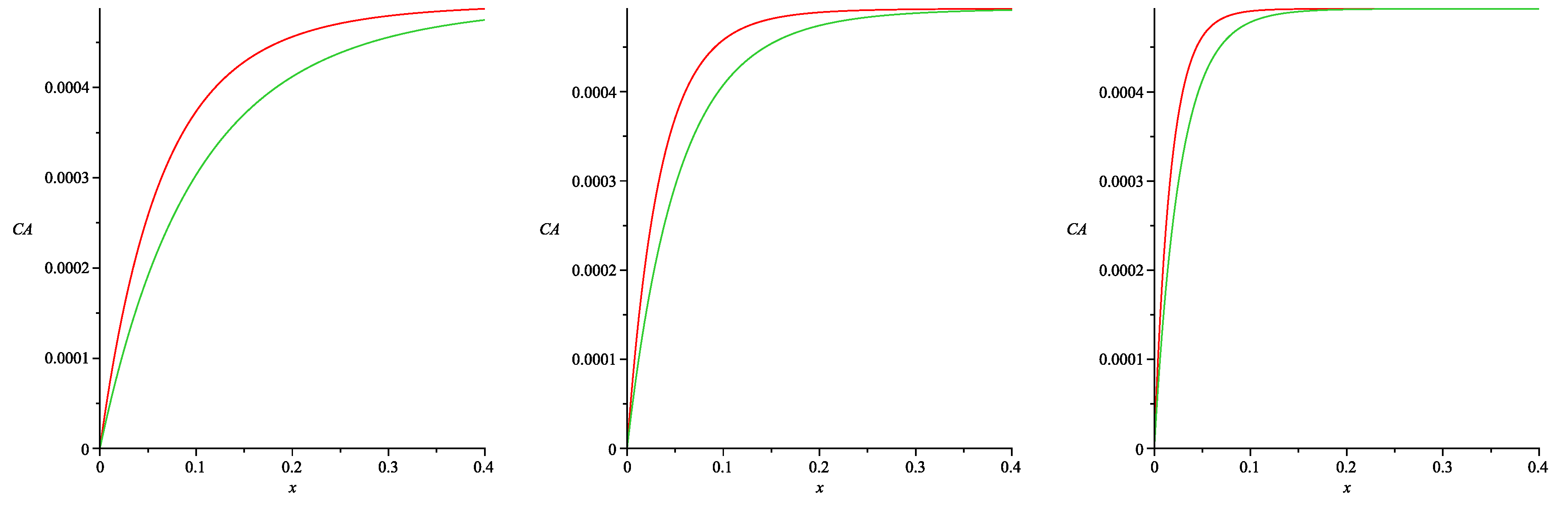The results are partly presented in Figure 4.

The phase plane for the variables ${\sigma }_{TG}$ and ${\sigma }_{CG}$ pictured in Figure 4(left) shows the domain, in which the difference between ultrafiltration derived via Formulae (47)–(50) and one calculated without restrictions (30) by numerical simulations is less than $10\%$ (it was assumed that such exactness is reasonable for practical applications). The phase planes pictured in Figure 4(center, right) show how this domain depends on dialyzate pressures, which usually vary from 3 mmHg–12 mmHg. The phase plane in center shows the domain obtained for the dialyzate pressure $P_D=7.5$ mmHg, while the plane on the right presents the domain for the lowest admissible pressure $P_D=3$ mmHg. Thus, one may conclude that the assumption about the equality of the reflection coefficients in the tissue and in the capillary wall provides good approximation for the case of nonequal coefficients if their values are within the respective domains. However, depending on the values of the dialyzate pressure these domains can be either larger (for low pressures) or smaller (for high pressures).

5. Numerical Results and Their Application for Peritoneal Dialysis

Here we present numerical results based on the formulae derived in Section 3 under the condition that the albumin transport plays an important role in the transport process between the tissue and the peritoneal cavity. Our aims are to estimate the role the fractional albumin volume ${\nu }_A$ in this process (when the stationary phase occurs i.e., the steady-state solutions describe the fluid-solute transport) and to compare the results obtained with some experimental data. In order to do this, we fix the following large value of the Staverman reflection coefficients for albumin: ${\sigma }_{TA}={\sigma }_A=0.5$.

As was explained in Section 2, we assume that the function ${\nu }_A$ depends on the space variable x in a more complicated way than it is usually assumed, i.e., ${\nu }_A=\gamma \nu$ ($\gamma <1$) [9,11]. Here we take:

$${\nu }_A\left(x\right)={\nu }_{A0}-{\nu }_{A1}{e}^{{\alpha }_{A}x}$$

(53)

where:

$${\nu }_{A0}=\frac{{\nu }_{Amax}{e}^{{\alpha }_A}-{\nu }_{Amin}}{e^{{\alpha }_A}-1},{\nu }_{A1}=\frac{{\nu }_{Amax}-{\nu }_{Amin}}{e^{{\alpha }_A}-1}$$

in order to obtain ${\nu }_{Amin}$ and ${\nu }_{Amax}$ for $x=1$ and $x=0$, respectively. The fractional fluid void volume $\nu \left(x\right)$ is still assumed of the form (37). In the numerical results presented here, we take ${\alpha }_A=1$, $\alpha =5$, ${\nu }_{Amin}=0.01$, ${\nu }_{Amax}={\nu }_{max}$. This means that a critical value of ν, for which only glucose and small metabolites are transported within tissue, while large molecules are completely blocked, is close to ${\nu }_{min}$, while the fractional void volume $\nu ={\nu }_{max}$ is sufficiently large in order to allow the albumin transport in the same way as small metabolites are transported.

We remind the reader that the standard assumption is ${\nu }_A=\gamma \nu$ ($\gamma <1$). Now we want to show that the results obtained for two different ways of the function ${\nu }_A$ prescription can be essentially different.

First of all, we need to specify the constant γ, because the coefficients arising in (53) are already given. Taking into account that the formulae for ${\nu }_A$ and ν reflect the tissue elasticity (during peritoneal transport), the part of the whole tissue allowing the albumin transportation should be a fixed number, hence ${\int }_0^L{\nu }_A\left(x\right)dx=constant$. Thus, using Formulae (37) and (53), the correctly-specified value γ should be calculated as follows:

$$\gamma =\frac{I_1}{I_2},I_1={\int }_0^L{\nu }_A\left(x\right)dx,I_2={\int }_0^L\nu \left(x\right)dx,$$

(54)

and, as a result, one obtains $\gamma \approx 2/3$. The graphs of the functions given by Formulae (37), (53) and ${\nu }_A=\frac{2}{3}\nu$ is presented in Figure 5. All of the other parameters were fixed and are listed in Table 1.

Because of the reasons explained in Section 4, we concentrated on different values of the coefficient ${\sigma }_G$. Namely, we want to establish how the albumin concentration and the albumin clearance from the tissue depend on the values of ${\sigma }_{TG}$ and the profile of ${\nu }_A$. It should be noted that the fluid flux from blood to the tissue $q_U$ and the fluid flux across the tissue $j_U$ do not depend on the albumin transport parameters (see Formulae (40)–(41)); hence these fluxes can be still found in the same way as above (see Section 4).

Figure 6 presents the spatial distributions of the albumin concentration in the tissue depending on the values of ${\sigma }_{TG}$. These curves were obtained by the numerical simulation of ODE (52) with the boundary Conditions (25)–(26). The interstitial albumin concentration $C_A$ increases rapidly with the distance from the peritoneal surface to the constant steady-state value of $C_A^{*}$ (see Formula (15) in [11]). One easily notes that the albumin concentration is essentially smaller in the case of ${\nu }_A$ (53) than in the case ${\nu }_A=\frac{2}{3}\nu$, provided the values of ${\sigma }_{TG}$ are small. This essential difference occurs in the tissue layer, which has the width $0.1-0.4$ $cm$ (depending on the ${\sigma }_G$ value). However, both profiles of the albumin concentration practically coincide for large values of ${\sigma }_{TG}\ge 0.01$. Analogous simulations have been done for a wide range of parameters arising in Formulae (37), (53) and (54), and the results were similar. Thus, we conclude that the fractional albumin volume ${\nu }_A$ cannot be assumed as a linear function of ν (at least for small values of the Staverman reflection coefficients for glucose and large ones for albumin).

The albumin clearance is an important characteristic of dialysis and the rate of the albumin clearance is defined by the albumin flux across the tissue, $j_A(t,x)$. This rate can be calculated in a similar way to the total fluid outflow (ultrafiltration), and

$$C{l}_A=\frac{5·{10}^3\left|j_A\left(0\right)\right|}{C_{AB}},\left[C{l}_A\right]=mL/min$$

where $5·{10}^3$ $c{m}^2$ is the surface area of the contact between dialysis fluid and peritoneum [9], and the function $j_A\left(x\right)$ is defined by (8) and is negative (similarly to $j_U\left(0\right)$) at a vicinity of point $x=0$ (the albumin concentration $C_A\left(x\right)$ and the fluid flux $j_U\left(x\right)$ are already known).

The albumin clearance rates $C{l}_A$ and the ultrafiltration rates $Uf$ for different values of the coefficient ${\sigma }_G$ are presented in

Table 2. The albumin clearance and ultrafiltration in peritoneal dialysis. All of the values of the parameters are taken from Table 1 and ${\sigma }_A={\sigma }_{TA}=0.5$.

Staverman Reflection	Ultrafiltration	Albumin
Coefficients ${\sigma }_G={\sigma }_{\mathrm{TG}}$	$Uf$	Clearance ${Cl}_A$
0.001	$0.12$ $mL/min$	$0.10$ $mL/min$
0.002	$0.61$ $mL/min$	$0.24$ $mL/min$
0.003	$1.155$ $mL/min$	$0.44$ $mL/min$
0.005	$2.24$ $mL/min$	$0.88$ $mL/min$
0.010	$4.97$ $mL/min$	$1.99$ $mL/min$
0.015	$7.69$ $mL/min$	$3.11$ $mL/min$

. As it is well-known from experimental data $C{l}_A<Uf$, so that the results are plausible. Moreover, the albumin clearance rates $C{l}_A$ are growing when the coefficient ${\sigma }_G$ is increasing, and this again corresponds to the experimental data. However, one notes that the values of $C{l}_A$ are too high comparing to some experimental data [20], in which the rates $C{l}_A=0.05-0.10$$mL/min$ were measured. We assume that there are two main reasons leading to the above contradiction: (i) the fractional albumin volume ${\nu }_A$ can be essentially smaller than the one presented in Figure 5; (ii) the mathematical assumption(30) is too restrictive. In order to examine these reasons, one needs to do many numerical simulations and to provide a detailed analysis of the results obtained. We plan to do this in a forthcoming paper.

6. Conclusions

In this paper, the mathematical model for fluid transport in peritoneal dialysis, which was proposed in [11], was further studied and generalized. The model is based on a three-component nonlinear system of two-dimensional partial differential equations and the relevant boundary and initial conditions.

In order to show that the transportation of macromolecules (albumin is a typical example) essentially differs from the water and glucose transportation because of their large size we have introduced a new notion, fractional albumin volume ${\nu }_A$, which (like ν) depends on the hydrostatic pressure P; however, it is not assumed that ${\nu }_A=\alpha \nu$, as in previous studies. It should be noted that such a generalization means that so called effective diffusivities $\nu D_G$ and ${\nu }_A{D}_A$ are some independent functions of the hydrostatic pressure (generally speaking, the diffusivities $D_G$ and $D_A$ can also be some functions of the pressure P).

To find non-uniform steady-state solutions, the model was reduced to the boundary-value problem for a non-linear ODE system. It turns out that the system obtained can be essentially simplified under assumptions (30) about the equality of the Staverman reflection coefficients in the tissue and in the capillary wall, which demonstrates an interesting specific symmetry in the governing equations of the model. In order to obtain exact solutions in an explicit form, the exponential profiles for the fractional fluid void volume were used, which are much closer to the profiles arising in experimental data than the linear profiles used in [11]. As a result, the exact formulae (involving both elementary and hypergeometric functions) for the density of fluid flux from blood to the tissue and the fluid flux across the tissue were constructed.

New analytical results are compared to those obtained earlier and checked for their applicability for the description of transport during peritoneal dialysis. In Section 4, we have done this assuming the water and glucose transport and neglecting the albumin transport. In particular, we have shown that values of ultrafiltration calculated using new formulae are higher than those obtained earlier (for the same parameters but for linear profiles for the fractional fluid void volume ν); therefore they seem to be more plausible. However, one cannot directly compare these ultrafiltration values with experimental data because the Staverman reflection coefficients cannot be directly measured.

Using numerical simulations we established how the exact solutions found under pure mathematical assumption (about the equality of the Staverman reflection coefficients) differ from those numerically constructed without this assumption. In particular, we have shown that the assumption about this equality leads to the correct values of ultrafiltration provided these coefficients belong to a correctly-specified domain. Moreover, it was proven that the size of the domain essentially depends on the values of dialyzate pressure. Thus, the exact solutions obtained can be applied for a wide range of parameters arising in experimental data for peritoneal transport.

In Section 5, the albumin transport was taken into account using very high values of the Staverman reflection coefficients for albumin. This means that the albumin transport is an important component in solute transport. We have shown that the albumin concentration profiles are essentially different if one calculates those by a standard way, i.e., assuming that ${\nu }_A=\gamma \nu$ ($\gamma <1$), and by the introduction of the notion of the fractional albumin volume, i.e., the function ${\nu }_A$ does not depend linearly on ν, but is defined by the Formula (11). The relevant simulations have been done for different values of the Staverman reflection coefficients. As a result, one may claim that the above mentioned profiles coincide only for large values of ${\sigma }_{TG}$.

We have also calculated the albumin clearance $C{l}_A$ and the ultrafiltration rates $Uf$ (two very important characteristics of the peritoneal dialysis) in order to estimate the applicability of the results. The results obtained are qualitatively plausible, however quantitative rates of the albumin clearance are essentially higher than those arising in experimental studies. We aim to study possible reasons elsewhere.