Article

Investigating the Performance of a Fractal Ultrasonic Transducer Under Varying System Conditions

by
Euan Barlow
1,2,*,
Ebrahem A. Algehyne
1 and
Anthony J. Mulholland
1
1
Department of Mathematics and Statistics, University of Strathclyde, 26 Richmond Street, Glasgow G1 1XH, UK
2
Department of Management Science, University of Strathclyde, 199 Cathedral Street, Glasgow G4 0QU, UK
*
Author to whom correspondence should be addressed.
Symmetry 2016, 8(6), 43; https://doi.org/10.3390/sym8060043
Submission received: 22 January 2016 / Revised: 17 May 2016 / Accepted: 31 May 2016 / Published: 6 June 2016
(This article belongs to the Special Issue Symmetry and Fractals)

Abstract

:
As applications become more widespread there is an ever-increasing need to improve the accuracy of ultrasound transducers, in order to detect at much finer resolutions. In comparison with naturally occurring ultrasound systems the man-made systems have much poorer accuracy, and the scope for improvement has somewhat plateaued as existing transducer designs have been iteratively improved over many years. The desire to bridge the gap between the man-made and naturally occurring systems has led to recent investigation of transducers with a more complex geometry, in order to replicate the complex structure of the natural systems. These transducers have structures representing fractal geometries, and these have been shown to be capable of delivering improved performance in comparison with standard transducer designs. This paper undertakes a detailed investigation of the comparative performance of a standard transducer design, and a transducer based on a fractal geometry. By considering how these performances vary with respect to the key system parameters, a robust assessment of the fractal transducer performance is provided.

Graphical Abstract

1. Introduction

Ultrasonic sensors are used for imaging in various fields of science and engineering, ranging from fetal scanners [1,2,3,4,5] to non-destructive testing and evaluation of nuclear power stations [6,7,8]. Ultrasound transducers are the components which generate and detect sound waves, converting electrical energy to mechanical energy (and vice versa) through vibrations induced on the transducer [9]. The standard design for ultrasonic transducers, referred to here as the homogeneous or Euclidean design, consists of one or more components configured in a periodic array [9,10]. Due to their regular geometry, these transducers can attain strong resonating performance at the harmonics of the transducer; however, the range of frequencies around each harmonic which have strong sensitivity—the bandwidth—can be limited. In contrast, many natural ultrasound systems can transmit and receive ultrasound over a wide range of resonating frequencies, with species such as bats and flies endowed with extremely sensitive transmission and reception sensitivities over exceptional bandwidths [11,12,13,14]. It is noteworthy that these naturally occurring transduction systems display complex geometries.
The structure of the paper is as follows: in Section 2, fractal transducers are introduced and the mathematical model which describes the performance of these transducers is summarised in Section 3, Section 4.1 investigates the performance of both the standard and fractal sensors as the material parameters are varied, Section 4.2 investigates the performances over a range of geometrical design parameters, Section 4.3 combines these to examine the transducer performance over a range of design and material parameters, with discussion and conclusions provided in Section 4.4 and Section 5, respectively.

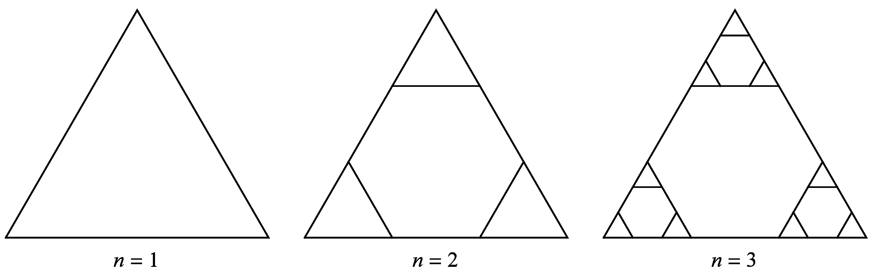
2. Fractal Transducer Design

The desire to bridge the gap between man-made and natural ultrasound systems has motivated the investigation of fractal transducers [15,16]. Piezoelectric transducers produce sound waves through vibrations of the piezoelectric materials from which they are composed. Whereas the homogeneous geometry of the standard (Euclidean) device is characterised by a single length scale, the natural systems exhibit a wide range of intricate geometries and often have resonators over a range of length scales, providing the natural systems with a far broader frequency range [11,12,13,14,17]. Fractals are mathematical structures constructed by iteratively repeating a governing geometrical pattern at each scale [18,19]. Fractals therefore consist of a range of length scales, and provide a natural framework to approximate the complex geometry of a natural ultrasound system. The Sierpinski gasket is a classical example of a self-similar fractal, where the repeating pattern consists of four equilateral triangles inside a larger equilateral triangle at each scale of this structure [20]. The Sierpinski gasket lattice (see Figure 1) is the lattice counterpart of the Sierpinski gasket [21,22], and provides a structure which is amenable to analysis. The performance of a fractal transducer with a geometry based on the Sierpinski gasket lattice has been investigated previously [16], and the performance of this device compared with a standard (Euclidean) device [23].

3. Mathematical Model for the Fractal Transducer

Algehyne and Mulholland [23] derive and interrogate the governing equations for a transducer with geometry defined by the Sierpinski gasket lattice. These derivations stem from consideration of the general tensor equations for the lattice, which provides a 3D framework to model the global dynamics of this transducer. This enables investigation of the transverse modes of the device, where the electric field operates within the plane of the lattice and the displacement acts out of this plane. The Sierpinski gasket lattice transducer is similar to a 1-3 connectivity composite transducer although for simplicity it is composed of one material and the second phase, which is normally a polymer, is just void space. The device has a single electrode on its top surface and a single electrode on its bottom surface. It is therefore modelled as a one dimensional single element sensor; the internal microstructure being homogenised using a renormalisation approach. The resulting characteristics of each mode of transducer operation are given in the form of analytical expressions, which enables rapid calculation of the transducer performance.
The full process which gives rise to the analytical forms of the Sierpinski gasket lattice transducer operating characteristics is detailed in Algehyne and Mulholland [23] and is omitted here for brevity; however, the approach is summarised here for completeness. The wave velocity in the piezoelectrically stiffened material can be expressed as c T = μ T / ρ T , where μ T = c 44 ( 1 + e 24 2 / ( ε 11 c 44 ) ) is the piezoelectrically stiffened shear modulus, ρ T is the density in the piezoelectric material, and c 44 , e 24 , and ε 11 are, respectively, elements of the stiffness tensor, the piezoelectric tensor and the permittivity tensor in the constitutive piezoelectric equations [24]. The ratio of the cross-sectional area of each edge of the Sierpinski gasket transducer to the length of the edge is denoted by ξ at each generation level, the capacitance of the transducer is then C 0 = ξ ε 11 / ( 2 n 1 ) and the parameter q = q ( n ) = i 2 π ( c T ( 2 n 1 ) / L ) 1 f is the scaled frequency f at fractal generation level n. The electrical load parameters a = Z P / ( Z 0 + Z P ) and b = Z 0 Z P / ( Z 0 + Z P ) combine the parallel electrical impedance load, Z P , and the series electrical impedance load, Z 0 . The mechanical impedance is given by Z L = ρ L c L ξ L / ( 2 n 1 ) for the load on the front face of the transducer, Z B = ρ B c B ξ L / ( 2 n 1 ) for the backing material, and Z T = ρ T c T ξ L / ( 2 n 1 ) for the transducer. The density is denoted ρ and the wave velocity is denoted c, with the subscripts L, B and T representing the front load, backing layer and piezoelectric material of the transducer, respectively.
A finite element methodology is employed by Algehyne and Mulholland [23], which gives rise to the Green’s transfer matrix, G, representing the Laplace transform of the vertex displacement throughout the Sierpinski gasket lattice when a unit impulse is applied. Exploiting the symmetries of the lattice reduces the Green’s transfer matrix to the pivotal elements
G 11 ( n ) = G ^ i i ( n ) + 2 G ^ j k ( n ) γ ^ m G 1 N ( n ) 1 G ^ i i ( n ) γ ^ 1 ,
G 1 N ( n ) = G ^ j k ( n ) ( 1 G ^ i i ( n ) γ ^ 1 ) ( 1 γ ^ m ( G ^ i i ( n ) + G ^ j k ( n ) ) ) 2 ( G ^ j k ( n ) ) 2 γ ^ 1 γ ^ m ,
G N N ( n ) = G ^ i i ( n ) + G ^ j k ( n ) γ ^ 1 G 1 N ( n ) + G ^ j k ( n ) γ ^ m G m N ( n ) 1 G ^ i i ( n ) γ ^ m ,
and
G m N ( n ) = G ^ j k ( n ) ( 1 + γ ^ 1 G 1 N ( n ) ( 1 + γ ^ m ( G ^ j k ( n ) G ^ i i ( n ) ) ) ) ( G ^ i i ( n ) γ ^ m 1 + G ^ j k ( n ) γ ^ m ) ( G ^ i i ( n ) γ ^ m 1 G ^ j k ( n ) γ ^ m ) ,
for any i , j , k { 1 , m , N } such that j k , where N = 3 n is the total number of vertices in the Sierpinski gasket lattice of generation level n, and m represents the vertex labelled ( N + 1 ) / 2 . The non-dimensional parameter γ ^ j ( n ) = η j ( n ) γ j , where
γ j = ( 1 q Z B Z T ) 1 , j = 1 ( 1 q Z L Z T ) 1 , j = m or N 0 otherwise
and
η j ( n ) = 4 3 2 15 q 2 , j = 1 1 + 1 3 ( 2 n + 1 1 ) + 11 15 × 2 n 30 2 n + 1 1 q 2 , j = m or N .
This methodology is then employed as the basis for a renormalisation approach [21,25,26,27,28], and the recursive relations required to populate Equation (1)–Equation (4) are defined as
G ^ i i ( n + 1 ) = G ^ i i ( n ) + 2 β 2 ( G ^ j k ( n ) ) 2 ( G ^ i i ( n ) + β ( G ^ i i ( n ) ) 2 β ( G ^ j k ( n ) ) 2 ) ( 1 + β G ^ i i ( n ) + β G ^ j k ( n ) ) ( 1 β 2 ( G ^ i i ( n ) ) 2 β G ^ j k ( n ) + β 2 ( G ^ j k ( n ) ) 2 ) ,
and
G ^ j k ( n + 1 ) = β ( G ^ j k ( n ) ) 2 ( 1 + β G ^ i i ( n ) β G ^ j k ( n ) ) ( 1 + β G ^ i i ( n ) + β G ^ j k ( n ) ) ( 1 β 2 ( G ^ i i ( n ) ) 2 β G ^ j k ( n ) + β 2 ( G ^ j k ( n ) ) 2 ) ,
for i , j , k { 1 , m , N } such that j k . The matrix G ^ ( n ) = ( A ^ ( n ) ) 1 , and at the first generation level A ^ i j ( 1 ) = α if i = j and β otherwise, where α = 4 + ( 8 q 2 / 5 ) and β = 2 / 3 + 11 q 2 / 30 .
A one dimensional spatial domain is added to the model at the top electrode (the front face) of the fractal design transducer in order to model the presence of a mechanical load. In a similar way another domain is added at the other electrode to model the transducer backing material. In transmission mode a voltage is applied to the transducer across the electrodes and the resulting displacement of the device produces a force in the front face mechanical load. The ratio of that force to the applied voltage is the transmission sensitivity. In reception mode an incoming mechanical wave is modelled in the front face mechanical load which then causes the transducer to vibrate. The ratio of the resulting voltage that is generated across the electrodes to this applied force is defined as the reception sensitivity. Both of these sensitivities are functions of the frequency of the applied voltage/force and so the associated sensitivity spectra can be plotted. Note that a similar approach is taken for the model of the standard (Euclidean) transducer. Algehyne and Mulholland [23] demonstrate for the fractal transducer design that the non-dimensionalised transmission sensitivity ψ is given by
ψ ( f ; n ) = F V / ζ C 0 = a Z L ( Z E + b ) μ T ξ C 0 K ( n ) ,
and the non-dimensionalised reception sensitivity ϕ is given by
ϕ ( f ; n ) = V F ( e 24 L ) = 2 ζ e 24 L σ 2 ξ μ T 1 ζ 2 a Z T ( σ 1 + σ 2 ) ( Z E + b ) q μ T 2 ξ 2 a Z T ( Z E + b ) q μ T ξ C 0 1 ,
where F is the force on the boundary of the transducer, V is the applied voltage and ζ = e 24 / ε 11 . In Equation (9) and Equation (10), the electrical impedance, Z E , is given by
Z E ( f ; n ) = Z T C 0 q μ T ξ 1 + ζ 2 C 0 μ T ξ ( σ 1 + σ 2 ) ,
with
K ( n ) = 1 q Z L Z T 1 η 1 ( n ) 1 q Z B Z T 1 G m 1 ( n ) + η m ( n ) 1 q Z L Z T 1 ( G m m ( n ) + G m N ( n ) ) + 1 ,
σ 1 = 1 q ( Z B / Z T ) 1 η 1 ( n ) ( G N 1 ( n ) G 11 ( n ) ) ,
and
σ 2 = 1 q ( Z L / Z T ) 1 η m ( n ) ( G N m ( n ) G N N ( n ) + 2 G 1 N ( n ) ) .
In Equation (9) the electrical impedance of the transducer ( Z E ) has to be of a similar order of magnitude as the lumped circuit electrical impedance b. Tuning the electrical circuit in this way ensures that there is efficient transfer of electrical energy to the device when it is operating in transmission mode. The electrical impedance is affected by the structure of the fractal geometry via the terms σ 1 and σ 2 that appear in Equation (11). Therefore, the second term in the brackets in Equation (11) has to be of order one. For a given piezoelectric material the material parameters are fixed but there remains freedom in the design parameters ξ and A r (which affects the capacitance C 0 ) to create this desired balance. When it is operating in reception mode, this tuning of the electrical impedances in the circuit ensures that the circuit is then sensitive to the changes in the electrical impedance of the transducer due to the mechanical vibrations. In Equation (10) both terms inside the large brackets must be of order one so that the vibrations of the device (conveyed by the terms σ 1 and σ 2 in Equation (13) and Equation (14)) have a marked effect upon the reception sensitivity. It is a relatively simple matter to identify a sensible choice of these parameters to design a sensitive transducer.
As outlined in Section 1, the motivation for investigating fractal transducers is to improve the operational performance of man-made transducers by providing higher amplitude sensitivities and a wider frequency range at which the transducer can attain high sensitivity. In Algehyne and Mulholland [23] the performance of a fractal ultrasonic transducer with geometry based on the Sierpinski gasket lattice at generation level 3 was compared with a standard (Euclidean) homogeneous design. By appropriate choices of the design parameters a fair comparison can be made between the fractal and the standard transducer design. This comparison focuses on the behaviour of the transducers around the thickness mode of operation. The standard design consists of a rectangular block of piezoelectric material of vertical thickness L that is polarised in this vertical direction. This is then electroded top and bottom where the area of each electrode is A r . A well-established linear systems model (one dimensional model) is used to predict the operating characteristics of this device [9,10] and so the length scale L dictates the resulting resonance frequency. Normally such transducers are 1-3 connectivity composites but to keep the analysis as simple as possible a single phase of piezoelectric material is used in this paper. The fractal device consists of a Sierpinski Gasket whose overall side length is also L. Positioning the electrodes as discussed above ensures that the distance between the electrodes for this device is also L, and that the area of each electrode footprint is A r . The device is composed of a single piezoelectric material whose polarisation is again aligned with the electrodes, and the renormalisation approach [21,25,26,27,28] as outlined above derives a one-dimensional model to predict the behaviour of this fractal device.
The models for the fractal transducer and the standard (Euclidean) transducer are therefore both one dimensional in space, and since both devices are resonating structures of thickness L then this length scale dictates the frequency at which the devices operate most efficiently. In three dimensions there will be some cross-talk between the pillars that make up the Sierpinksi gasket design and so there will be motion in all three directions and not just in the thickness direction; however, the one-dimensional transducer model will only capture this motion in a single direction. Additionally, since the transducer models are one dimensional then the acoustic field in the spatial domain at the front face of the transducers is one dimensional. As such the models presented in this paper cannot comment on the directivity pattern of the beam that each device creates. The same material was used for the front face material for both the fractal and the standard design; loss was not incorporated into this material model. A lossy material was used for the backing material and again the same material parameters were used for both designs.
Figure 2 and Figure 3 demonstrate the comparative performance of each type of transducer in transmission and reception modes of operation, for the piezoelectric material PZT-5H and with equivalent design characteristics. The fractal transducer design is shown to produce the desired behaviour with multiple resonance frequencies in each mode, ranging from approximately 2.3–2.9 MHz for the transmission mode. It is clear that the fractal transducer achieves a higher maximum amplitude for both transmission and reception modes of transducer operation; however, the spiked peaks evident in the fractal transducer sensitivity spectrum for each operating mode result in poorer bandwidth performance.
It is also of interest to examine the pulse-echo mode of transducer operation, where a single device transmits a signal and then receives the response. The amplitude at a given frequency for this mode of operation is defined here as the minimum of the transmission amplitude and the reception amplitude, where each sensitivity amplitude is normalised with respect to the maximum amplitude recorded in that mode of operation. The pulse-echo sensitivity at frequency f for Sierpinski gasket lattice transducer at fractal generation level n is then defined as
θ ( f ; n ) = min ψ ( f ; n ) max f ( ψ ( f ; n ) ) , ϕ ( f ; n ) max f ( ϕ ( f ; n ) ) .
Figure 4 compares the performance of each type of transducer in pulse-echo mode of operation, where both transducers are normalised (the denominators in Equation (15)) with respect to the maximum amplitude of the fractal transducer sensitivity. The transducer performance in pulse-echo mode is shown to be comparable to the performances displayed in Figure 2 and Figure 3, with the fractal transducer achieving a larger maximum amplitude and more peaks of high performance than the standard (Euclidean) transducer.

4. Investigating the Robustness of Transducer Performance

For fractal transducers to be widely utilised by the ultrasonic community further evidence of the efficacy of these devices is required, and the advantages of employing a fractal transducer design in place of a standard transducer design must be demonstrated beyond the single scenario portrayed in Figure 2, Figure 3 and Figure 4. This paper provides an investigation of transducer performance under a range of scenarios. In the first instance, the transducer performance is investigated as the material parameters are varied from the values given in Algehyne and Mulholland [23]; see Section 4.1. In Section 4.2 the second stream of investigation explores the impact on the transducer performance as the design parameters are varied. This investigation therefore explores the situation where the maximum performance is desired from a transducer which is constructed from a pre-selected (and accurately characterised) piezoelectric material. Section 4.3 goes on to combine both scenarios to investigate the performance of various alternatives for the design of each transducer when the piezoelectric material parameters span a range of values. Finally, discussion is provided in Section 4.4.
In the investigations which follow, the generation level of the Sierpinski gasket lattice transducer is set to three to provide a level of intricacy which could realistically be manufactured, and the piezoelectric material PZT-5H is considered to be the material of each transducer as this is commercially available and widely used in practice [30]. The performance of each transducer is measured in terms of the maximum gain (sensitivity), and the bandwidth to obtain a detailed understanding of the different aspects of the transducers performance. The maximum gain indicates the strongest possible response of the transducer and the bandwidth indicates the range of frequencies around this gain at which the transducer can still achieve acceptable performance. To ensure that a fair comparison was made between the two different designs (and indeed between different parameter settings within a single style of design) the decibel level at which the bandwidth was calculated at was kept fixed. This approach therefore mimics the real life situation whereby a transducer operator wants to know the range of frequencies that the transducer can operate at; that is, the frequencies at which it has a higher sensitivity than the noise level. The analytical expressions derived by Algehyne and Mulholland [23] for the sensitivity of the fractal transducer in transmission and reception modes, given by Equation (9) and Equation (10), enable rapid calculation of the transducer performance, and provide a means to perform detailed analysis under the various parameter settings in tractable computation time.

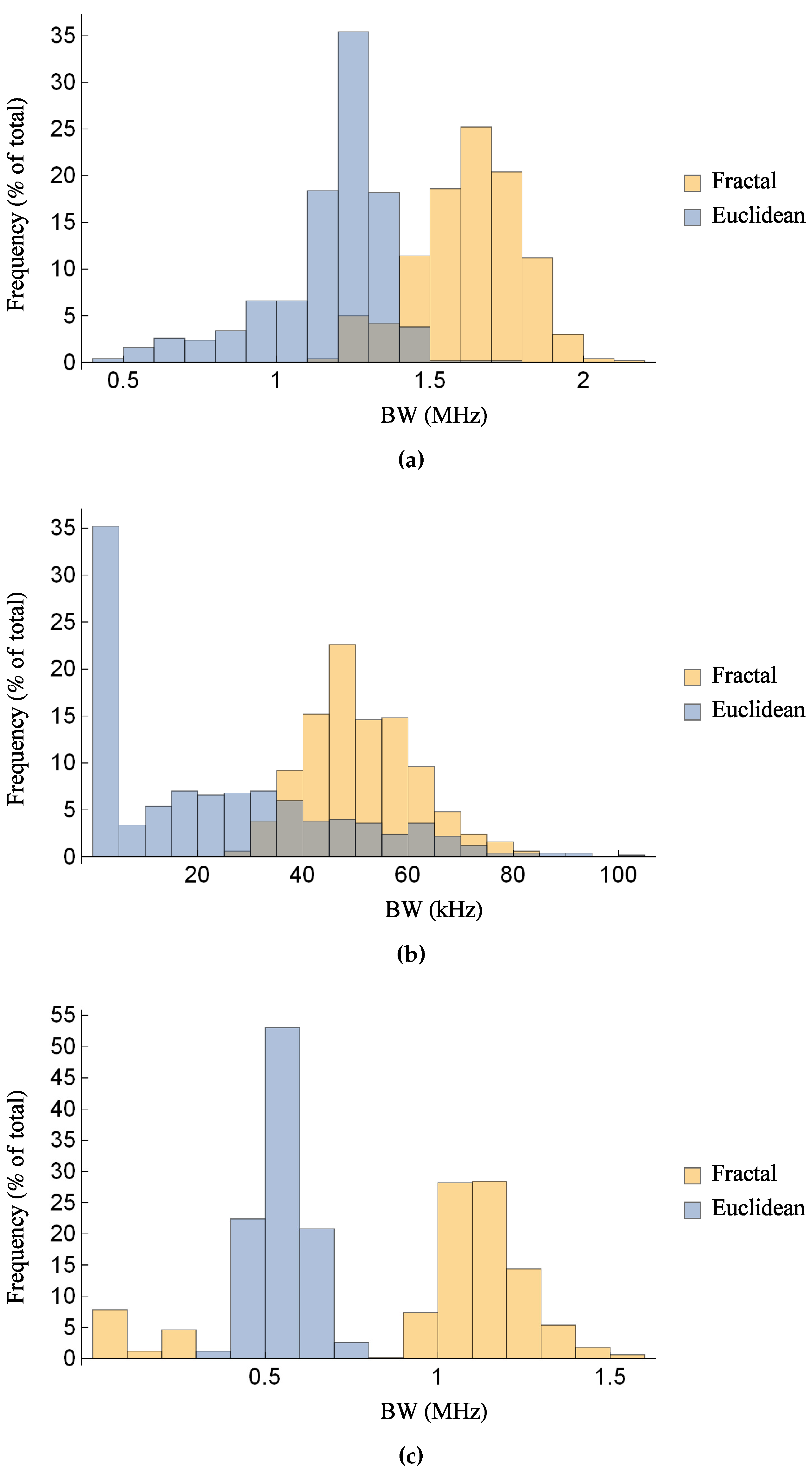
4.1. Transducer Performance with Uncertainty in the Key Material Parameters

This section explores the impact of uncertainty in the material parameter values on transducer performance. It can be seen from Section 3 that the piezoelectric material can be described by six parameters of interest. We denote this set of material parameters as p M = { c 44 , e 24 , ε 11 , ρ T , Z P , Z 0 } , and define P M as the corresponding set where each element is treated as a random variable. The expected values of this set, E [ P M ] , are defined as being equivalent to the corresponding advertised parameter values for the piezoelectric material PZT-5H, and are shown in Table 1. Each element of P M is modelled as a normal distribution with mean value equivalent to the corresponding value of E [ P M ] , and for consistency the standard deviation is set to 10% of the mean value of each parameter.
In Figure 5 and Figure 6 all parameters in the set of material parameters are treated as random variables, such that the set of material parameters are defined as p M = P M . The transmission, reception and pulse-echo sensitivities for the fractal transducer and the standard Euclidean transducer are compared for both performance measures discussed above. It is clear from Figure 2, Figure 3 and Figure 4 that the level of the noise threshold will have a substantial impact on transducer performance, and so a range of noise levels are investigated. The response of each transducer is simulated for 500 realisations of the uncertain material parameters, and the distribution of performance values from these simulations are presented as a box plot.
Figure 5 demonstrates that the fractal transducer achieves a higher maximum gain in transmission, reception and pulse-echo modes. As can be expected, there is relatively little variation between the responses at different noise floor levels. The median value for the gain of the fractal transducer (the line in the middle of each rectangle) is consistently 30%–40% above that for the standard Euclidean transducer. In comparison with the regular response pattern of the standard Euclidean design, the complex pattern for the fractal transducer shown in Figure 2, Figure 3 and Figure 4 gives rise to substantially more uncertainty (indicated by the larger length of the rectangles) regarding the maximum gain that is attained; however, the range of values observed for the fractal transducer (indicated by the vertical lines) is clearly superior to the range observed for the standard Euclidean design. Figure 6 compares the bandwidth range achieved by each transducer for transmission, reception and pulse-echo modes and various levels of noise threshold. The median bandwidth obtained by the fractal transducer is consistently higher than the standard Euclidean design in transmission mode. The degree of uncertainty in the bandwidth performance is generally comparable between both types of transducer, and the bandwidths decrease with increasing noise floor level as expected. A similar situation is shown for pulse-echo mode, with the fractal transducer consistently obtaining higher median bandwidths than the standard Euclidean design. In this case the standard Euclidean design shows less uncertainty in the bandwidth performance than the fractal transducer, however, the inter-quartile range of bandwidths (indicated by the frequencies which each rectangle spans) covers substantially higher frequencies for the fractal transducer, indicating that in the majority of cases the fractal transducer has obtained a superior bandwidth. In reception mode, however, the standard Euclidean design outperforms the fractal design in terms of median bandwidth at low noise levels with a larger distribution of performance values.
These investigations are continued in Figure 7 and Figure 8, where a more detailed comparison between the two transducer designs is provided by focusing on a single level of noise threshold. From Figure 6a,b, the bandwidths of both transducers in both transmission and reception modes of operation are roughly comparable for a noise floor level of 30 dB (see Figure 2), and this is therefore used as the level for the noise threshold in Figure 7a,b and Figure 8a,b. For the pulse-echo mode a noise floor level of 45 dB is used for the comparison as both transducers obtain reasonable bandwidth at this threshold, with performance starting to degrade (through more uncertain bandwidth performance) at higher noise floor levels, as shown in Figure 6c. As with Figure 5 and Figure 6, all material parameters in the set p M are treated as random variables. The transducers are examined in each mode of operation, and the distribution of the two performance measures over 500 simulations is shown in each case. For the levels of noise threshold investigated, the fractal transducer consistently outperforms the standard Euclidean design for each performance measure in each mode of operation. For the maximum gain, the fractal transducer exhibits a larger range over higher values in Figure 7a,b (transmission and reception modes, respectively), and higher values over a tighter range in Figure 7c (pulse-echo mode). In particular the standard (Euclidean) design achieves a relatively low gain in transmission mode and pulse-echo mode. In terms of bandwidth, Figure 8a,b demonstrate that the fractal transducer has a smaller range in both transmission and reception modes of operation, and covers higher bandwidth values. Furthermore, the distribution of bandwidth values for the standard Euclidean design is almost uniform in each case (discounting a peak at the lowest frequency-bin in the histogram), indicating that there is comparable probability of achieving any level of bandwidth in the range shown. Figure 8c shows that in pulse-echo mode the fractal transducer design obtains higher bandwidths than the standard Euclidean design in the majority of cases; however, in approximately 10% of cases the fractal transducer obtains a comparatively low bandwidth.

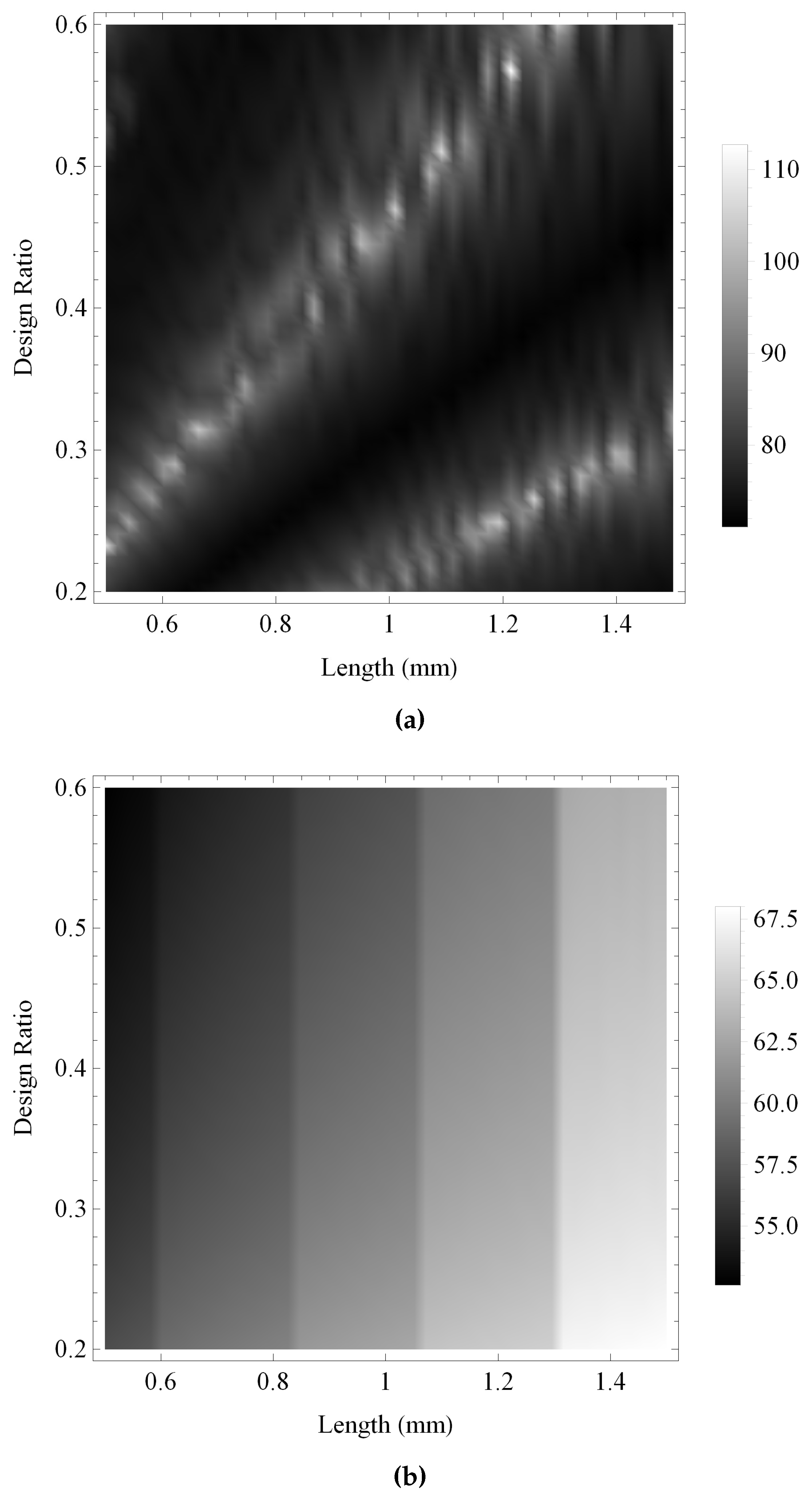
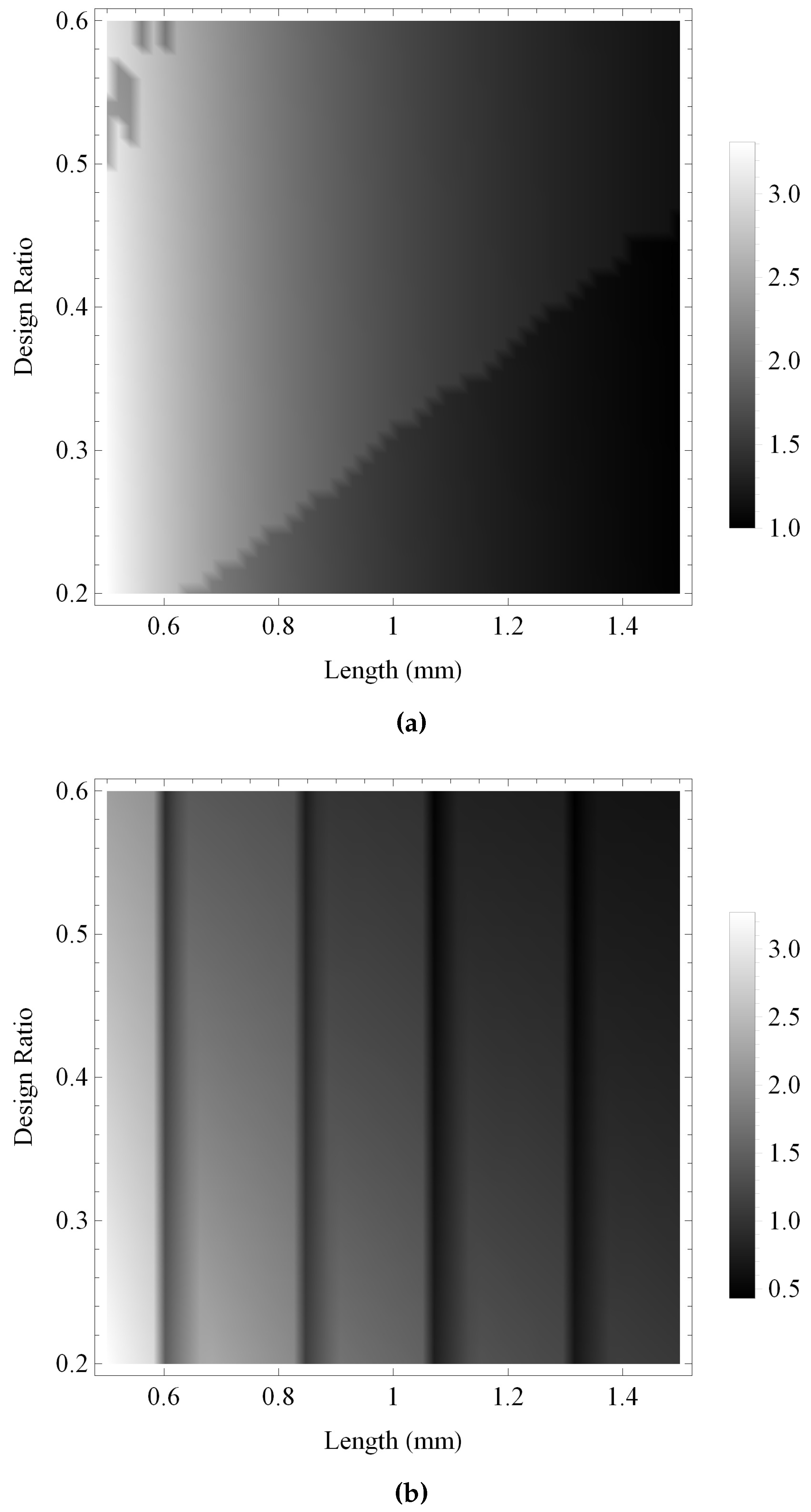
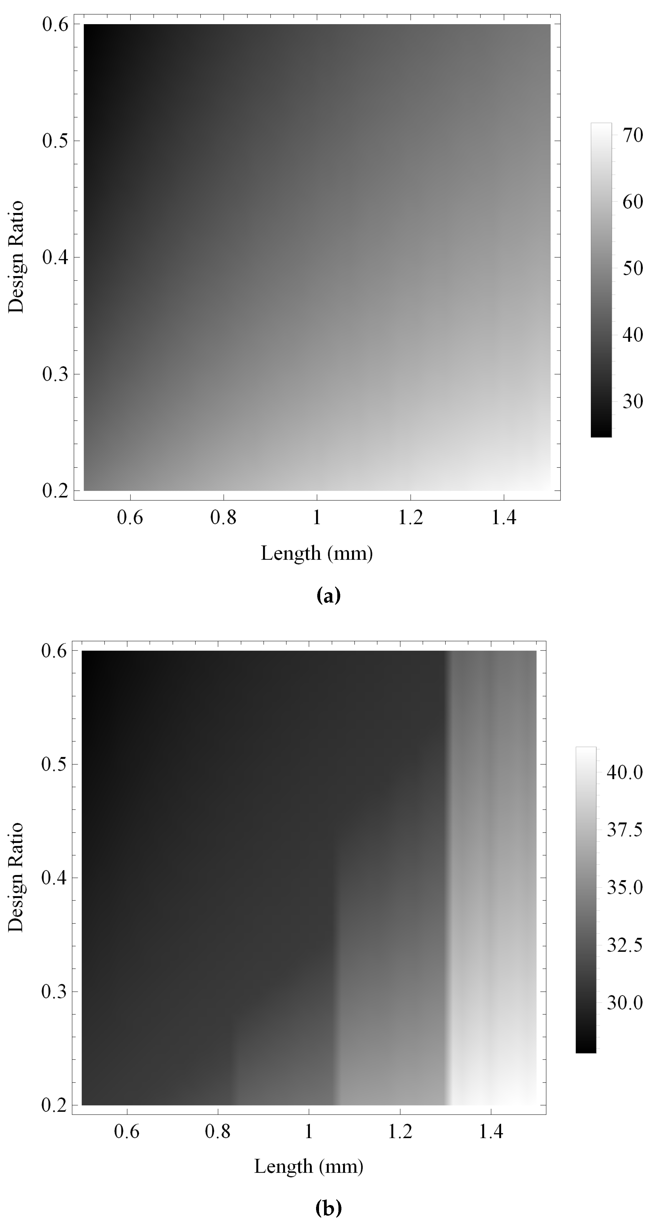
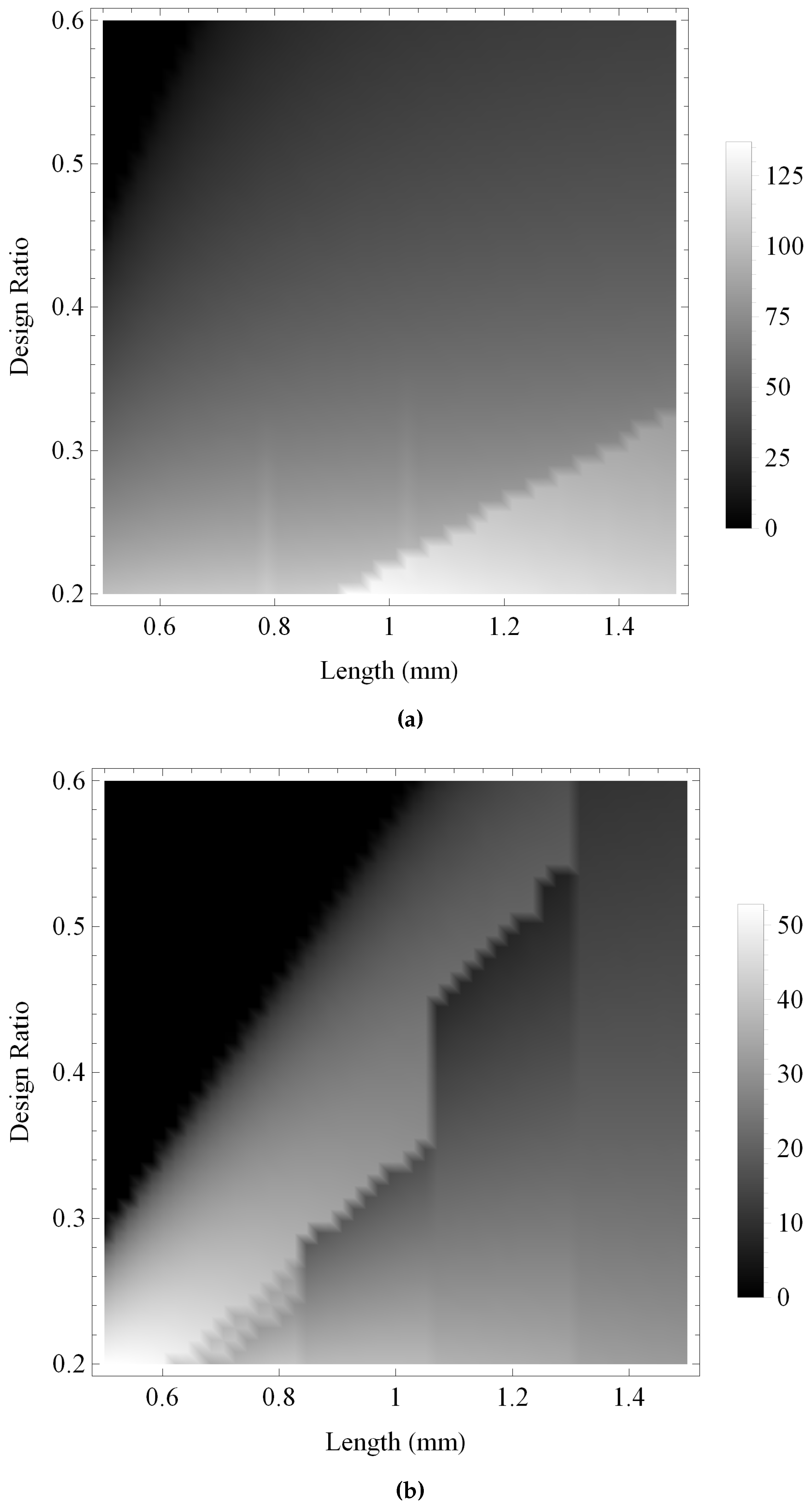
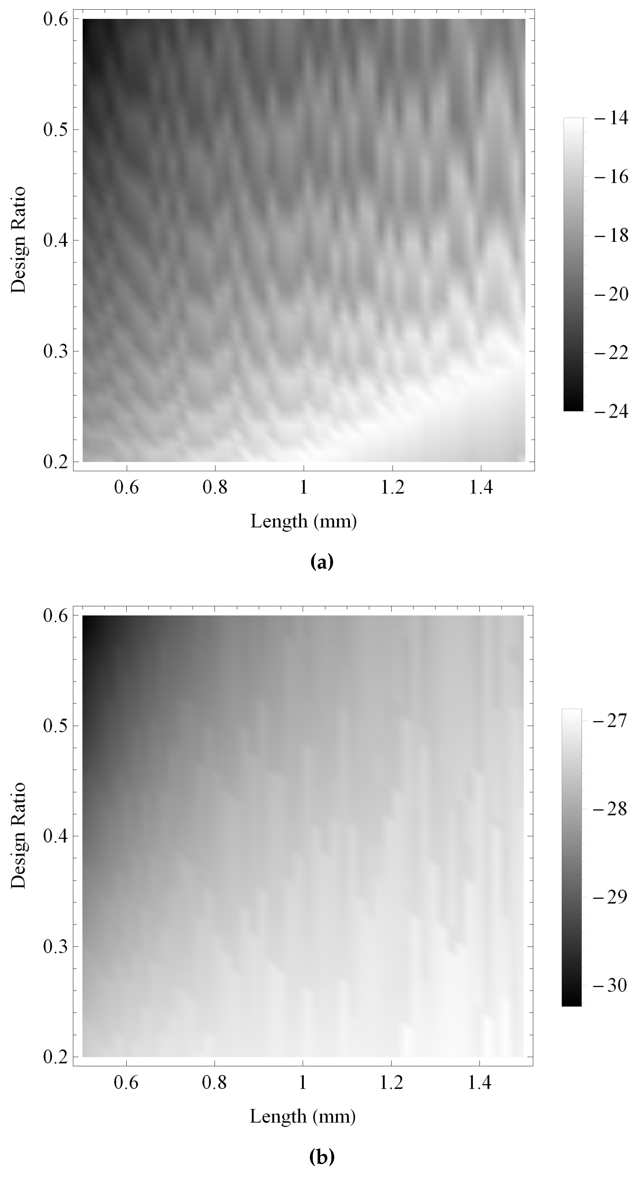
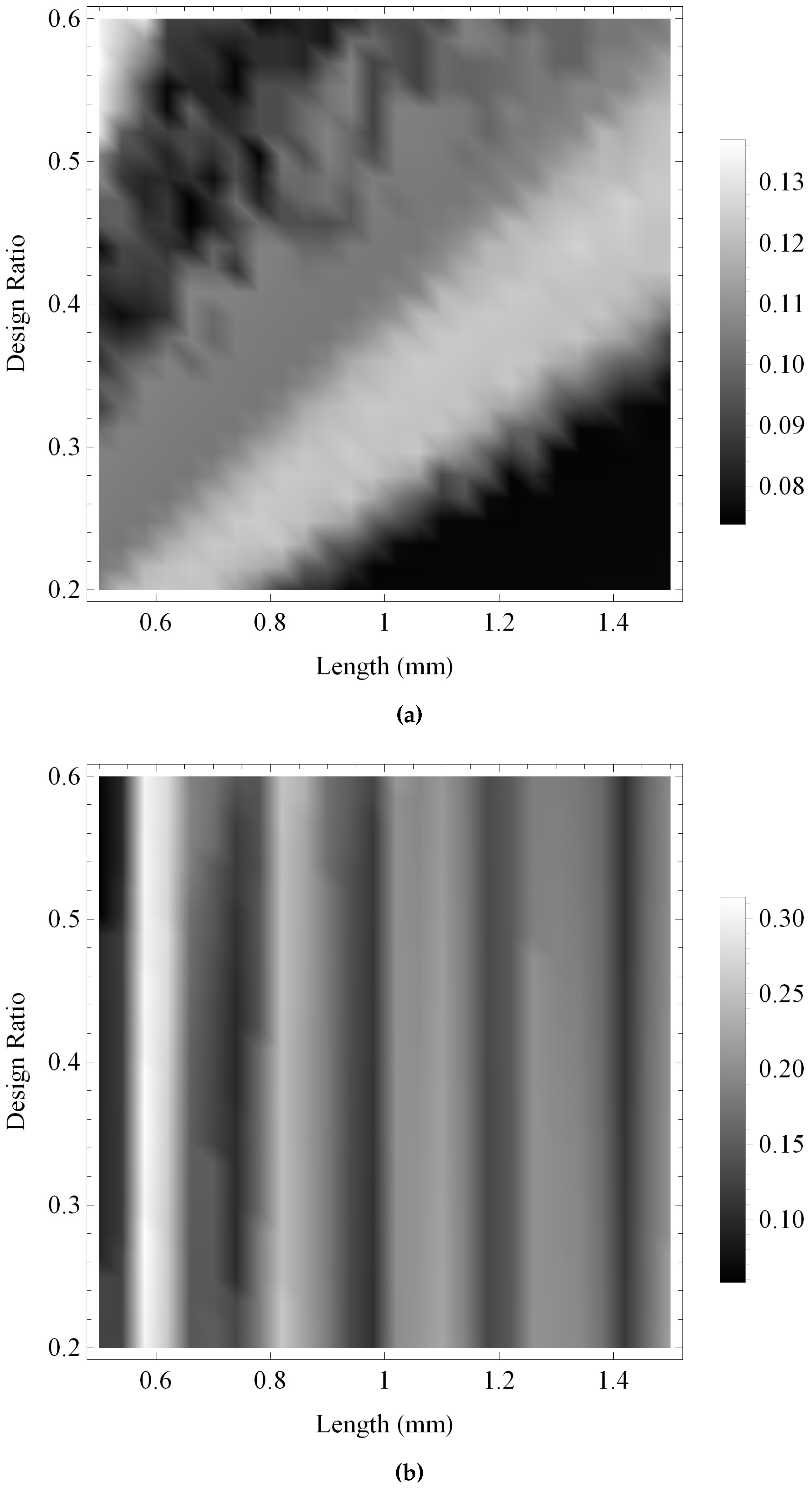
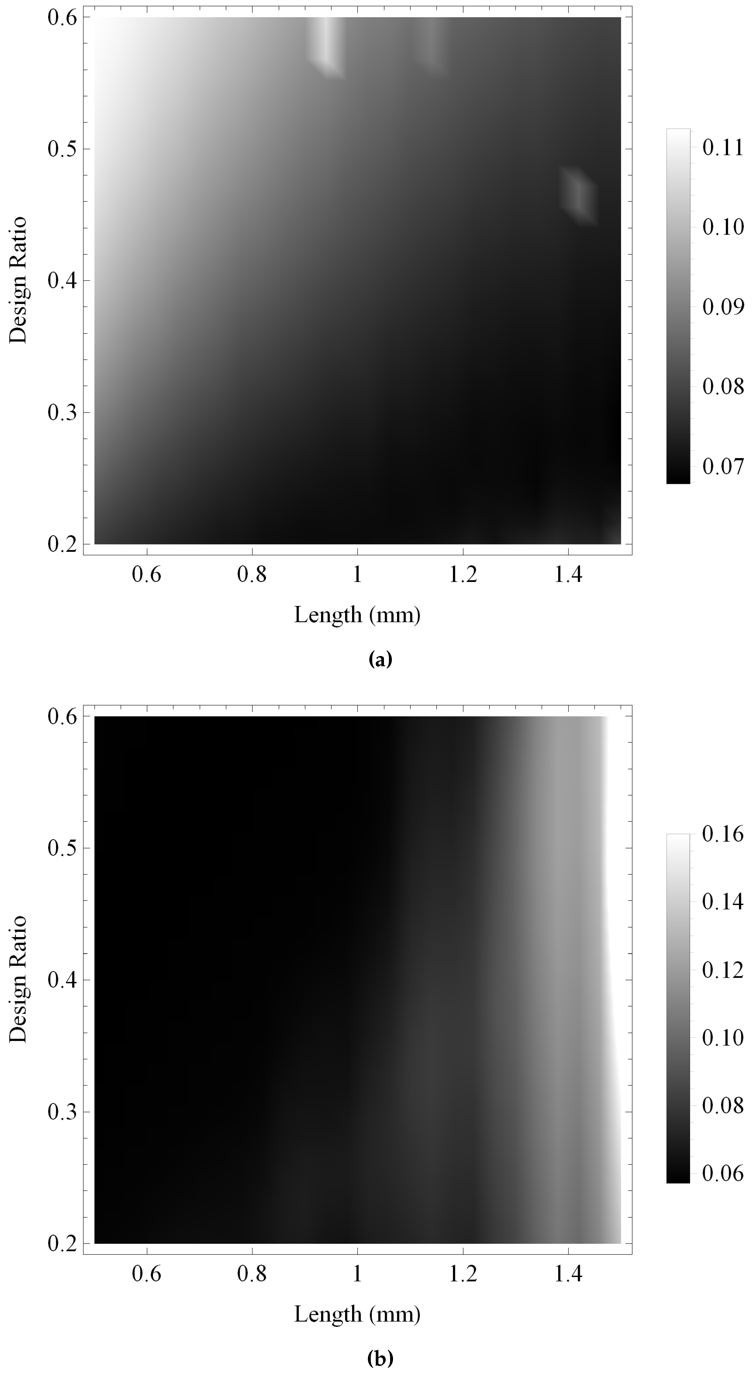
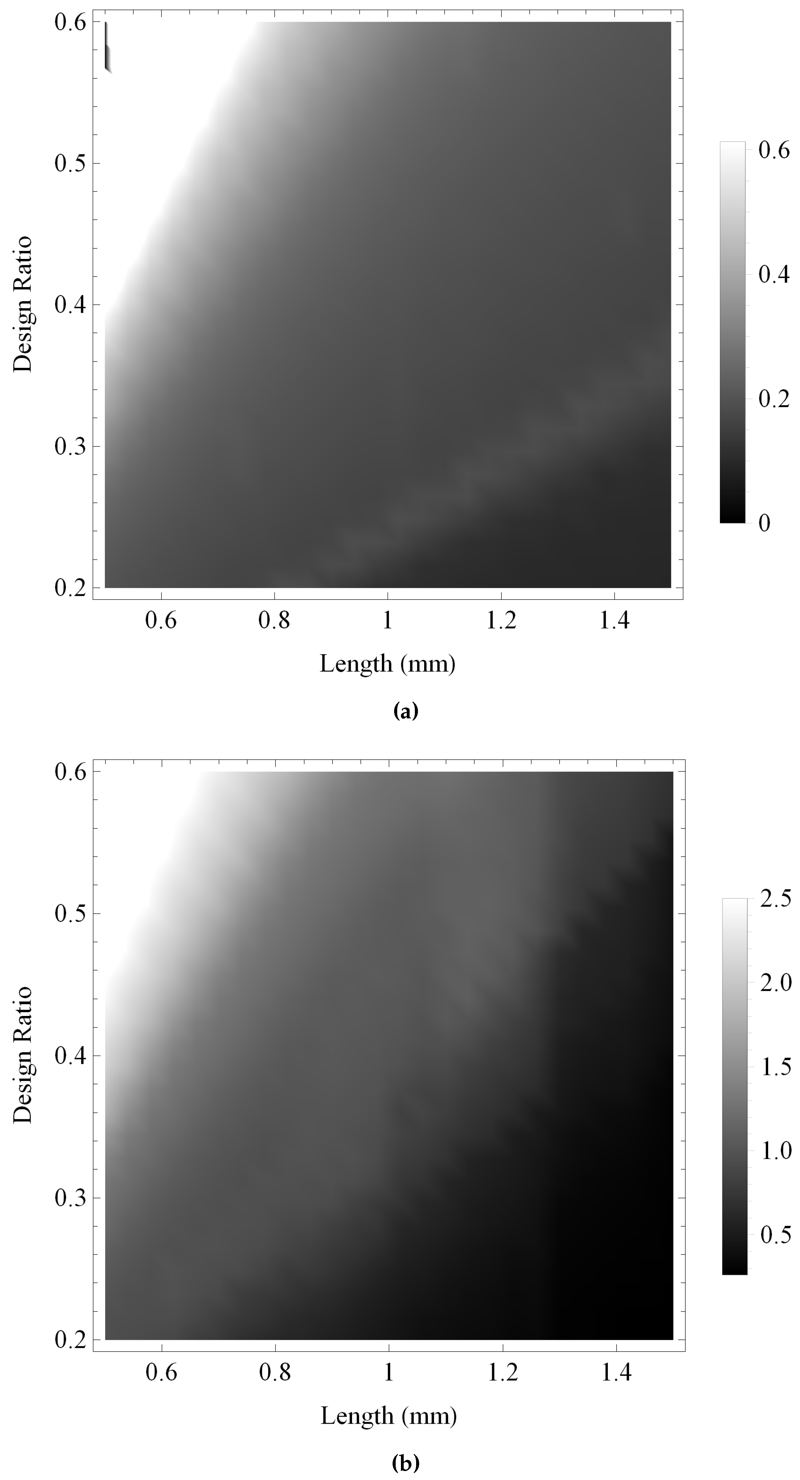
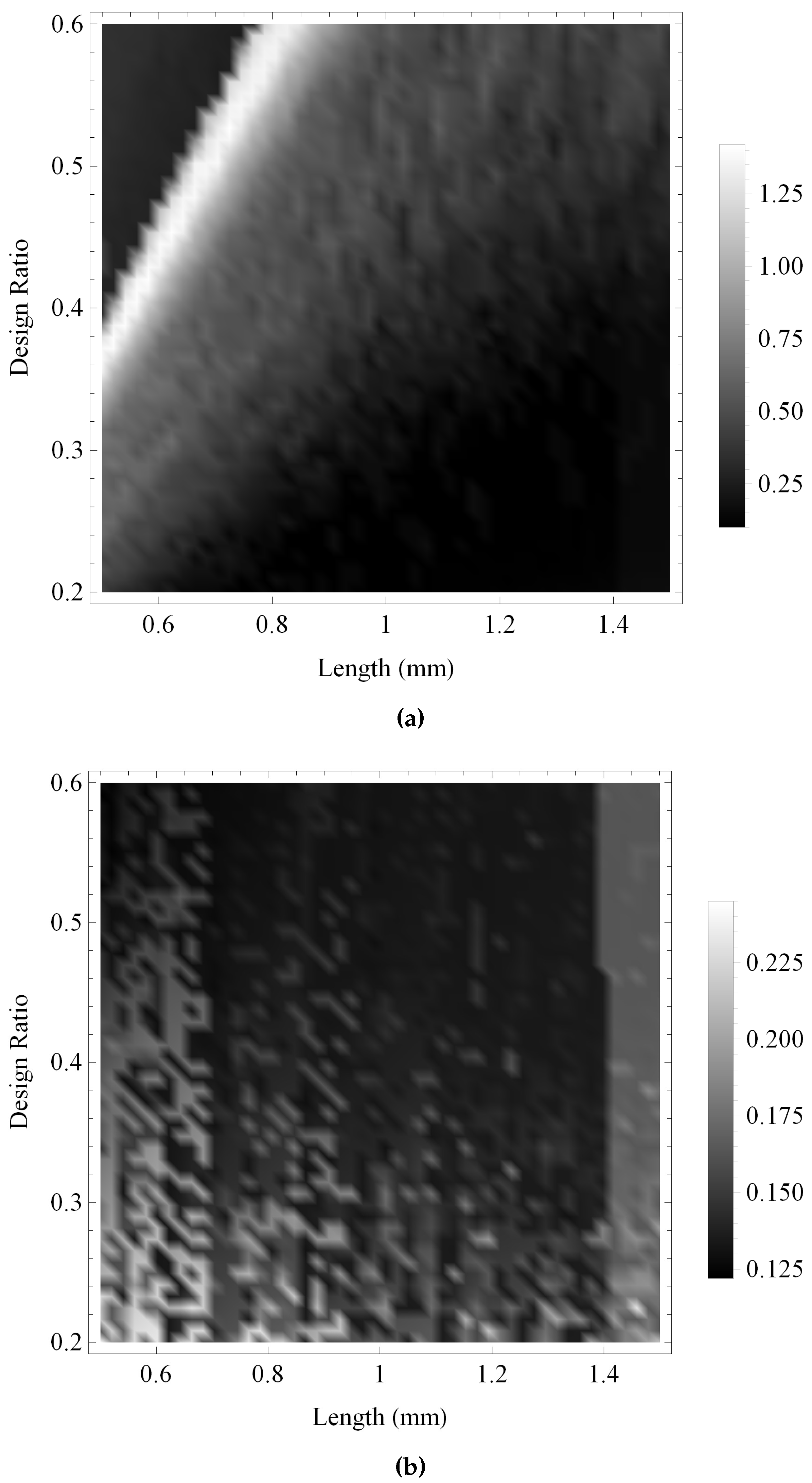
4.2. Transducer Performance under Various Design Regimes

The second stream of investigation is identifying the best geometrical design parameters available for the transducer, for a fixed set of material parameters. Both the fractal and the standard Euclidean transducers can be characterised by two key design parameters: the side length of the transducer, L, and the design ratio, ξ. In Figure 9 and Figure 10, the transmission sensitivity performance of both the fractal and the standard Euclidean transducers are calculated across ranges of these key design parameters. Each design parameter is explored over a range of ± 50 % of the baseline value in steps of 2%, where the baseline value is defined in Table 1. Performance is again measured using two metrics: maximum gain and the bandwidth of frequency responses above a fixed noise threshold. In Figure 9a, the maximum gain obtained by the fractal transducer in each design configuration is calculated, and a response surface is shown. There are two ridges of relatively high performance, with a main ridge extending from lower values of L and ξ to higher values of L and ξ, and a smaller ridge with L and ξ increasing from a region of mid-high L values and low ξ values. Numerous peaks along each ridge of high performance indicate focused regions of extremely high performance. The maximum gain of the standard Euclidean transducer is shown in Figure 9b to gradually decrease as the value of ξ increases, and steadily increase as L increases subject to several step changes in performance. In Figure 10, the bandwidth of the fractal transducer is shown to be relatively insensitive to changes in the design ratio, ξ, whereas the standard Euclidean transducer shows a gradual decrease in bandwidth with increasing ξ. Both types of transducer demonstrate an overall decrease in bandwidth with increasing side length, L; however, the standard Euclidean transducer shows distinct bands of higher performance separated by troughs of low performance.
Both performance measures of the reception sensitivity for the fractal and the standard Euclidean transducers are compared in Figure 11 and Figure 12. In Figure 11 the maximum gain of the reception sensitivity is shown for the fractal and standard Euclidean transducers. Both cases are relatively similar, demonstrating that the gain is lowest for higher values of L and lower values of ξ, and that the gain increases as L increases and as ξ decreases. The fractal transducer exhibits a reasonably smooth variation with both L and ξ, whereas the standard Euclidean transducer exhibits little variation in the region of higher ξ and lower L, with the banded step-like structure evident in Figure 9b and Figure 10b becoming increasingly observable for lower ξ and higher L. The bandwidth of the reception sensitivity for the fractal transducer is shown in Figure 12a, and has similar structure as shown in Figure 11a for the maximum gain. Three distinct regions of bandwidth are shown for the standard Euclidean transducer, with the same regions of lower performance and higher performance as shown in Figure 11b, but with an additional ridge at the intersection of the lower and higher performance regions exhibiting the highest bandwidth values.
Figure 13 and Figure 14 show the maximum gain and the bandwidth, respectively, of the pulse-echo sensitivity for the fractal and the standard Euclidean transducers. As with previous investigations, the maximum gain obtained by the fractal transducer is shown to be consistently larger than the standard (Euclidean) transducer in Figure 13, displaying an intricate performance surface with numerous regions of high performance throughout the design space and a general trend of higher performance towards regions of lower ξ and higher L. The bandwidth performance for the standard (Euclidean) design is shown in Figure 14b to be relatively consistent throughout the design space, with regions of highest performance for lower values of L. In comparison, the fractal transducer is shown to obtain higher bandwidths throughout the majority of the design space, with highest performance for lower L and ξ and two bands of comparatively lower performance in regions of lower L and higher ξ.

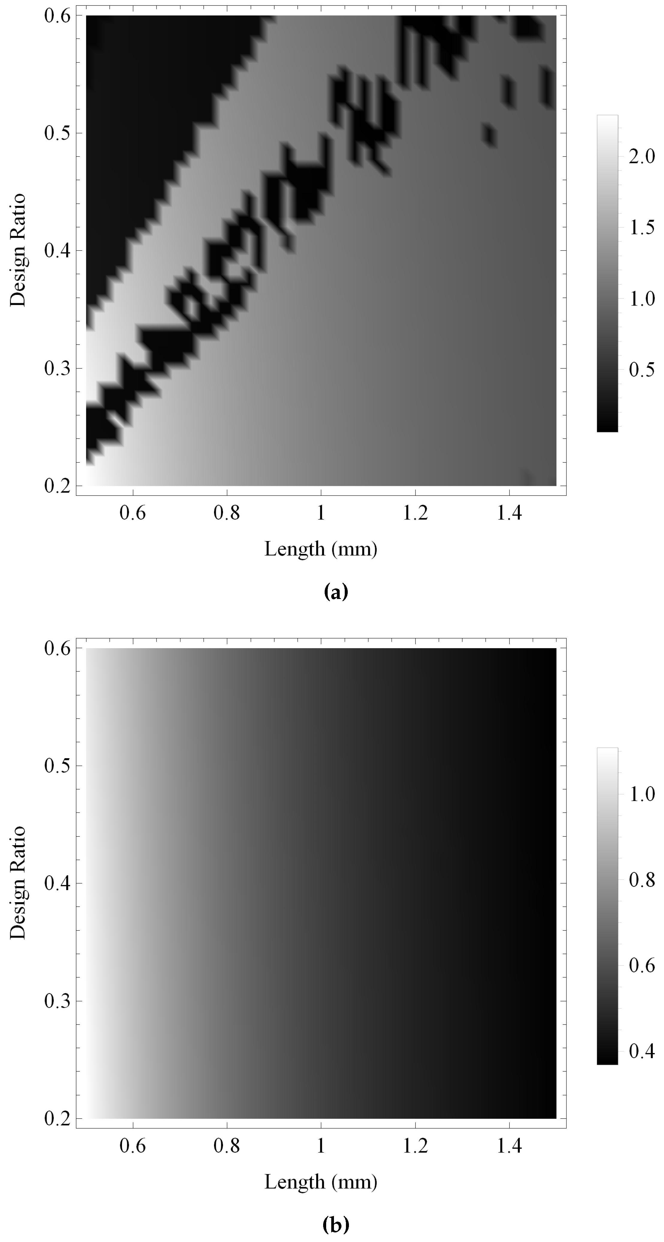
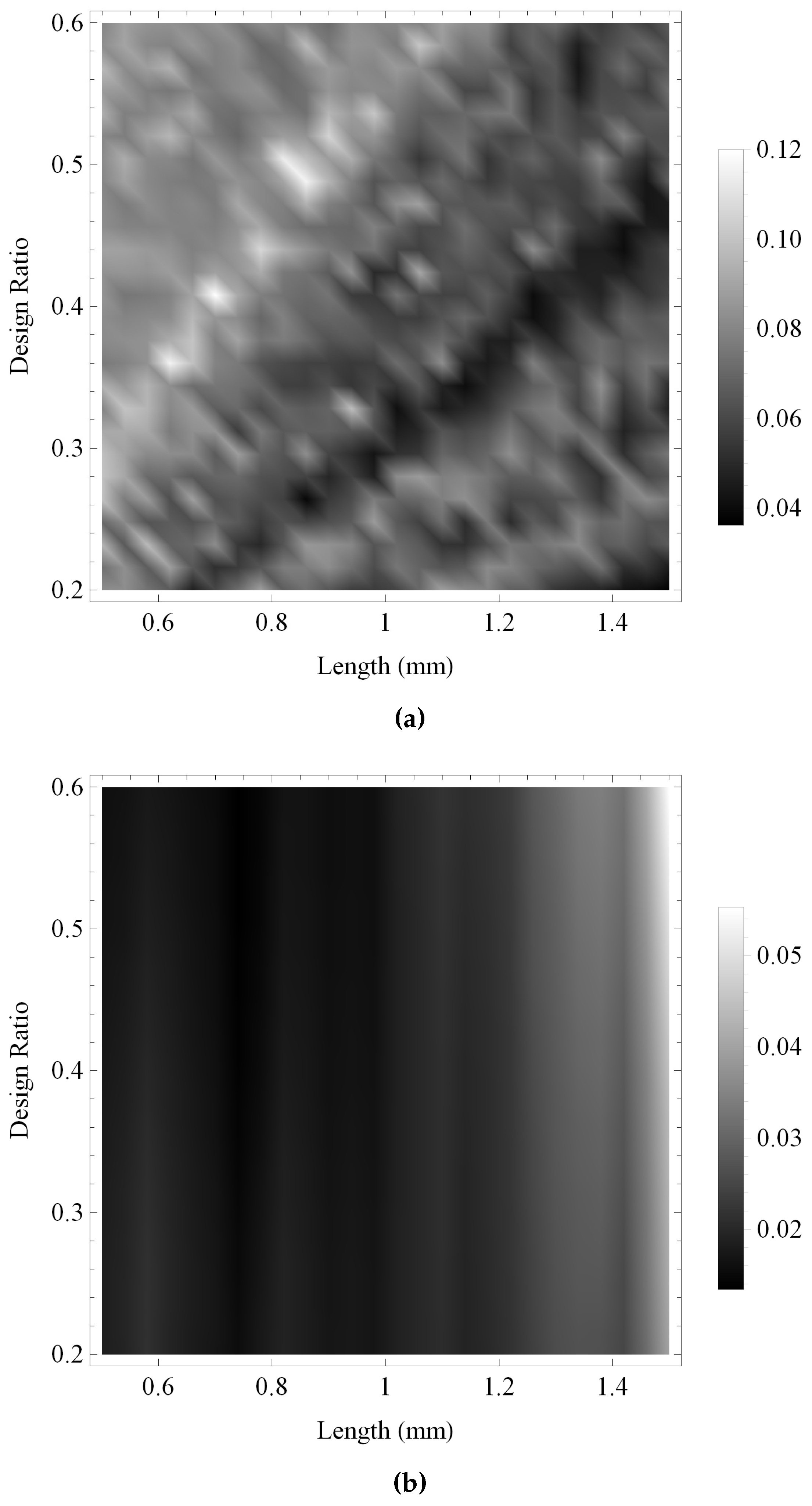
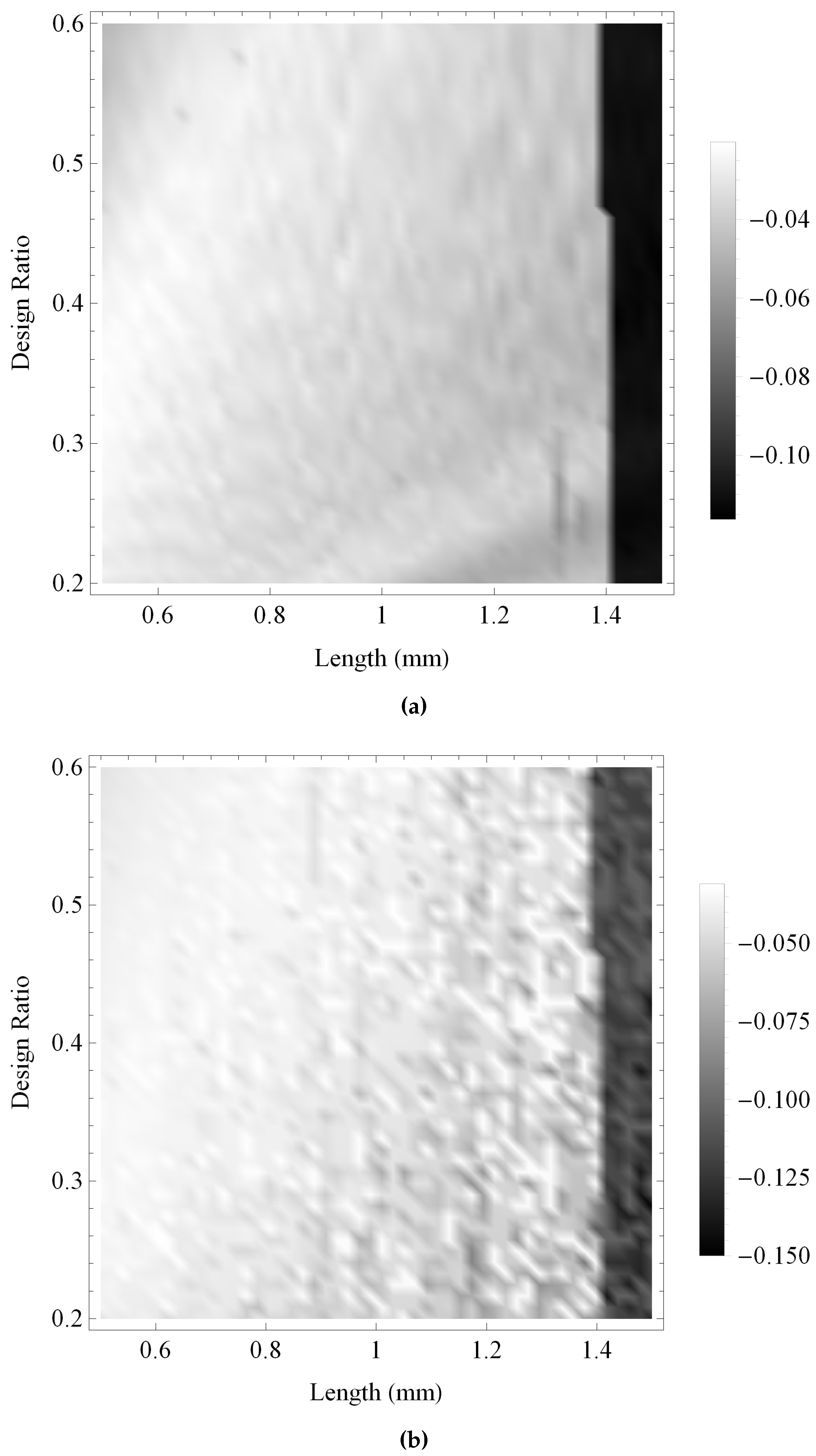
4.3. Transducer Performance under Various Design Regimes with Uncertainty in Material Parameter Values

The scenarios considered in Section 4.1 and Section 4.2 are combined here, to consider the problem of optimising the transducer performance with uncertain material and geometric design parameters. The key piezoelectric material parameters are defined as in Section 4.1, with each parameter described by a normal distribution centered on the expected value with a standard deviation of 10% of this value. The key design parameters are defined as in Section 4.2, with each parameter varied across a range extending from 50% less than the baseline value to 50% more than the baseline value. The results are shown in Figure 15, Figure 16, Figure 17, Figure 18, Figure 19 and Figure 20, where the performance of each transducer design is measured for 100 realisations of the key material parameters for the two performance metrics in transmission, reception and pulse-echo modes. These figures show the coefficient of variation—defined as the standard deviation divided by the mean—and provide a normalised measure of the uncertainty in transducer performance, with greater absolute values indicating greater uncertainty. In each case, the mean of a particular performance measure in a particular mode of operation for each transducer is comparable to that shown in the corresponding figures in Section 4.2.
In Figure 15 the maximum gain in transmission mode of the fractal transducer and the standard Euclidean transducer are examined. Both transducers demonstrate relatively low levels of variability in performance, with deviations of approximately 12% and 5% of the mean value for the fractal transducer and the standard Euclidean transducer, respectively. In each case the level of uncertainty has a complex behaviour throughout the space of design configurations and does not match directly with performance, although the highest performance regions are generally associated with the highest uncertainty.
In Figure 16 the bandwidth achieved by both transducers in transmission mode is compared. As with Figure 15, the regions of higher uncertainty do not map directly onto regions of higher performance, with a complex uncertainty structure displayed by both transducers. In each case the level of uncertainty has increased from Figure 15, and the fractal transducer has reduced uncertainty at up to 13% of the mean value in comparison with up to 30% of the mean value for the standard Euclidean transducer. Both transducers display relatively low uncertainty in regions of high bandwidth.
The levels of uncertainty in the maximum gain achieved by both transducers in reception mode are compared in Figure 17. In this case, the uncertainty in the standard Euclidean transducer response generally follows the behaviour of the performance with highest levels of uncertainty (at approximately 13% of the mean value) at the regions of highest performance. The fractal transducer exhibits a maximum uncertainty of approximately 8% of the mean value; however, the behaviour of the uncertainty surface is in contrast to the behaviour of the performance surface, and there is approximately 5% deviation from the mean value at the regions of highest performance.
In Figure 18 the uncertainty in the bandwidth performance of each transducer in reception mode is compared. There are regions of extremely high uncertainty for both transducers, where the skewed distribution of the bandwidth values results in extremely large coefficients of variation. These large uncertainties arise in regions where the amplitude of the gain is less than the noise floor level, and therefore no bandwidth is recorded, for the majority of realisations of the material parameter values. A small number of these realisations produce a gain marginally above the noise floor level, however, and a small number of non-zero bandwidths are therefore recorded and skew the resulting mean bandwidth values. To aid the display of these results, Figure 18a,b have both been thresholded at a coefficient of variation of one; however the maximum coefficient of variation is over seven in each case. For the fractal transducer the regions of high uncertainty are associated with the regions of extremely low bandwidth, and there is comparatively low uncertainty throughout the higher performance regions. In contrast, the regions of high uncertainty are widespread for the standard Euclidean transducer and coincide with regions of higher performance.
Figure 19 compares the level of uncertainty in the maximum gain for both transducers in pulse-echo mode. In each case, the level of uncertainty is approximately 5% of the mean value for the majority of transducer designs; however, both the fractal and the standard Euclidean transducer are shown to have a region of comparatively high uncertainty (at approximately 10% of the mean value) for L greater than approximately 1.4 mm. In Figure 20 the levels of uncertainty in the bandwidth are compared for pulse-echo mode of operation. For the standard Euclidean transducer this is shown to be relatively consistent, at approximately 15% of the mean bandwidth for the majority of transducer designs. The fractal transducer is shown to have a ridge of comparatively high uncertainty cutting through the upper left quadrant of Figure 20a. This ridge coincides with regions of lowest performance in terms of bandwidth, and further investigation reveals that this level of uncertainty can be attributed to a number of material parameter realisations achieving substantially larger bandwidths than is the norm for these transducer designs.

4.4. Discussion of Transducer Performance

The results of Section 4.1, where the design parameters are fixed and there is uncertainty in the material parameter values, demonstrate that the fractal transducer is consistently predicted to produce a high-level of performance. This performance is ultimately shown to be superior to the performance of the standard Euclidean transducer with respect to each performance measure. The significance of these results is that the fractal transducer is shown to robustly deliver a superior performance to the standard Euclidean transducer.
In Section 4.2 the material parameters are fixed at their expected values and a range of design configurations are examined, with both the fractal and the standard Euclidean transducers yielding interesting performance surfaces. The fractal transducer demonstrates substantially larger regions of high performance with respect to both gain and bandwidth than the standard Euclidean transducer. In designing a transducer, experimentalists would therefore have greater likelihood of producing a high-performance transducer by adopting a fractal design.
The problem of designing a transducer when the material properties of the piezoelectric material are uncertain is considered in Section 4.3. In the majority of cases the standard Euclidean transducer exhibits higher levels of uncertainty in performance and the extent of overlap between high uncertainty and high performance is more prevalent, in comparison with the fractal transducer. The only exception is for the maximum gain in transmission mode where both transducers show comparatively low uncertainty, and the uncertainty related to the standard Euclidean transducer performance is lower than that of the fractal transducer. The significance of these results is that the regions of high performance for the fractal transducer are more resilient to uncertainties in the material parameters, when compared with the standard Euclidean transducer.
The results of Section 4.1, Section 4.2 and Section 4.3 show that the fractal transducer can be expected to consistently produce a superior level of performance in comparison with the standard Euclidean transducer, and that this high performance is robust to changes in material properties and is achievable for a wide range of design configurations. These transducers therefore have the potential to deliver a step-change in transducer performance, and can lead to substantially more accurate ultrasound systems.

5. Conclusions

An investigation into the performance of ultrasonic transducers has been presented, with comparison between a standard (Euclidean) transducer design with a homogeneous structure, and a transducer design inspired by the high-performance ultrasound systems observed naturally in species such as bats and moths. Fractal geometry has recently been considered as a mechanism to mimic the complex and intricate structure of these natural ultrasound systems, and this work builds upon the work of Algehyne and Mulholland [23] who derived analytical expressions for the response of a fractal transducer. Utilising these analytical expressions provides an assessment of the transducer performance, and enables a large number of scenarios to be investigated in a tractable computing time. This makes it possible to ascertain the robustness of this performance as the system parameters vary.
Two situations which arise in the real-world development of transducers are considered: in the first situation the values of the key parameters which describe the piezoelectric material of the transducer are varied, and in the second situation the key design parameters of the transducer are varied in order to obtain the optimal transducer performance. The investigations of the first situation are presented as an interrogation of transducers constructed from one particular piezoelectric material (PZT-5H); however, these investigations could additionally be used to guide experimentalists in the design of novel high-performance piezoelectric materials by identifying the material parameter values that maximise the transducer response and are most robust to uncertainty. The second situation is a natural stage of the design process, where a transducer will be designed to provide the best possible performance. Transducers for which high performance is only attained for small ranges of design parameters are more challenging to optimise, and as a result the performance of these transducers can be more variable.
The fractal transducer is shown to outperform the standard (Euclidean) transducer. The fractal transducer is demonstrated to consistently achieve higher levels of performance over large ranges of the design variables, and has more resilience to uncertainties in the material parameters, particularly in the regions of high performance. As a result, the fractal transducer is shown to have the potential to bridge the gap between the current capability of man-made transducers and naturally occurring systems, and could give rise to a new generation of accurate and resilient transducer designs.

Acknowledgments

This work was supported by the Engineering and Physical Sciences Research Council, grant reference EP/I033424/1. Additionally, the authors gratefully acknowledge the support given by the Ministry of Higher Education, University of Tabuk in Saudi Arabia and the Royal Embassy of Saudi Arabia in UK.

Author Contributions

A.J.M. conceived and directed the program of work; A.J.M. and E.B. designed the investigations; E.A.A. developed the SG transducer model and wrote the computer code to simulate its transmission/reception sensitivities; E.B. wrote the computer code to perform Monte Carlo simulations of the transducer model, performed the simulation investigations, and analysed the plots that portray the outputs from these investigations; A.J.M. provided the physical interpretation and contextualisation of these outputs; E.B., A.J.M. and E.A.A. wrote the paper.

Conflicts of Interest

The authors declare no conflict of interest.

Abbreviations

The following abbreviations are used in this manuscript:
A ^ ( 1 ) Matrix used to construct G ^ ( 1 )
A r Cross-sectional area of each edge of the Sierpinski gasket transducer (m 2 )
a Z P / ( Z 0 + Z P ) (ratio of electrical impedances in the circuit (non-dimensional))
b Z 0 Z P / ( Z 0 + Z P ) (ratio of electrical impedances in the circuit (Ω))
C 0 The capacitance of the transducer (F)
c 44 An element of the stiffness tensor of the piezoelectric material (N·m 2 )
c T The (piezoelectrically stiffened) wave velocity in the SG ( n ) ( 3 ) lattice (m·s 1 )
c L Wave speed in the front load (m·s 1 )
c B Wave speed in the backing layer (m·s 1 )
e 24 An element of the piezoelectric tensor of the piezoelectric material (C·m 2 or N·V 1 ·m 1 )
fThe natural frequency
G j i ( n ) The Green’s transfer matrix given by Equation (1)–Equation (4) (non-dimensional)
G ^ ( n ) Recursive relations utilised for the renormalisation approach, given by Equation (7) and Equation (8) (non-dimensional)
hLength of each edge of the Sierpinski gasket transducer (m)
K ( n ) Non-dimensionalised parameter given by Equation (12)
LThickness of transducer (m)
mThe vertex labelled ( N + 1 ) / 2
N = 3 n The total number of vertices in the SG ( n ) ( 3 ) lattice
nThe fractal generation level
qScaled frequency
Z B Mechanical impedance of backing layer (N·s·m 1 )
Z L Mechanical impedance of the front load (N·s·m 1 )
Z T Mechanical impedance of the transducer (N·s·m 1 )
Z P Parallel circuit electrical impedance load (Ω)
Z 0 Series circuit electrical impedance load (Ω)
Z E ( f ; n ) Electrical impedance of the SG ( n ) ( 3 ) lattice given by Equation (11) (Ω)
αNon-dimensionalised parameter equal to 4 + ( 8 q 2 / 5 )
βNon-dimensionalised parameter equal to 2 / 3 + 11 q 2 / 30
γ j Non-dimensionalised parameter given by Equation (5)
γ ^ j ( n ) Non-dimensionalised parameter equal to η j ( n ) γ j
ε 11 Element of the permittivity tensor of the piezoelectric material (F·m 1 )
ζ e 24 / ε 11 (V·m 1 )
η j ( n ) Non-dimensionalised parameter given by Equation (6)
μ T The (piezoelectrically stiffened) shear modulus (N·m 2 )
ξ A r / h (m)
ρ B Density of the backing layer (kg·m 3 )
ρ L Density of the front load (kg·m 3 )
ρ T The density of the piezoelectric material (kg·m 3 )
σ 1 Non-dimensionalised parameter given by Equation (13)
σ 2 Non-dimensionalised parameter given by Equation (14)
ϕ ( f ; n ) 
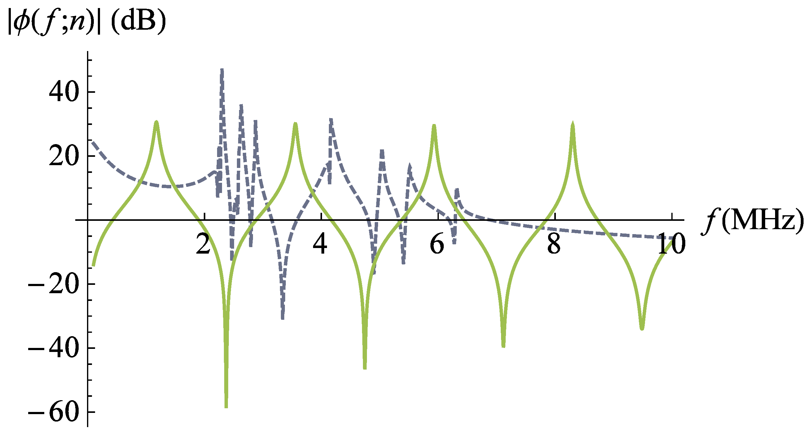
The non-dimensionalised reception sensitivity given by Equation (10)
ψ ( f ; n ) 
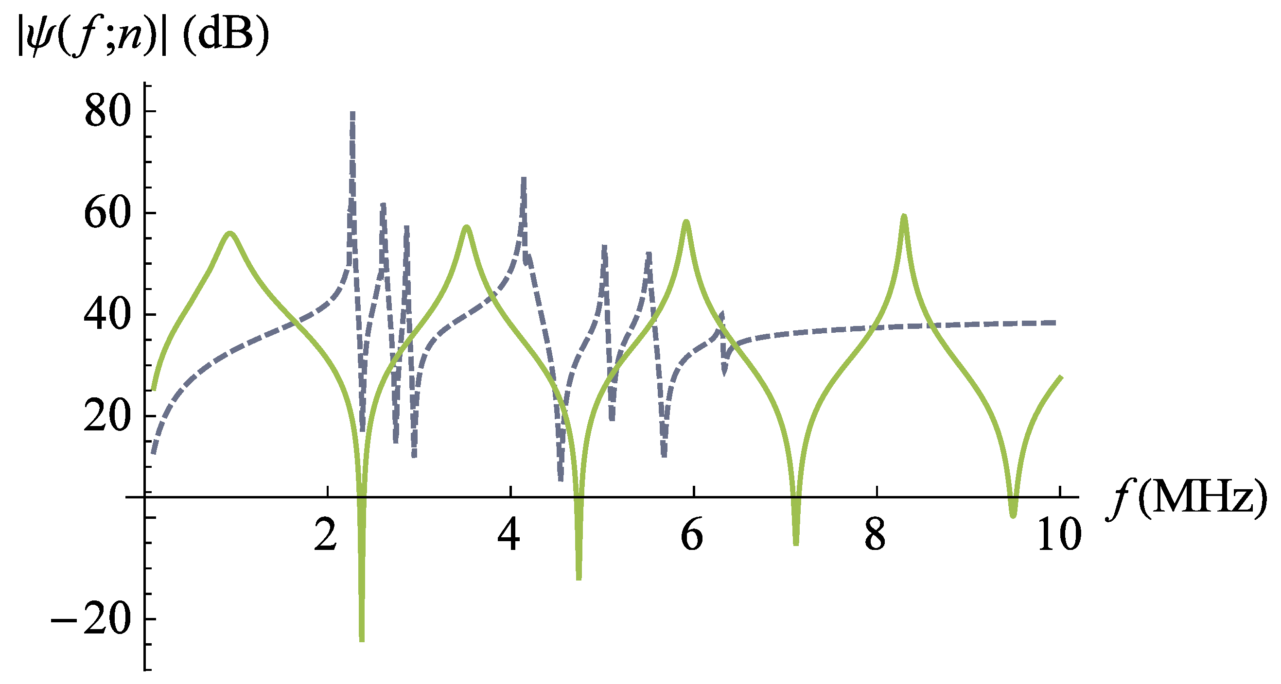
The non-dimensionalised transmission sensitivity given by Equation (9)

References

  1. Alfirevic, Z.; Stampalija, T.; Medley, N. Fetal and umbilical Doppler ultrasound in normal pregnancy. Cochrane Database Syst. Rev. 2015, 4, CD001450. [Google Scholar] [PubMed]
  2. Bricker, L.; Medley, N.; Pratt, J.J. Routine ultrasound in late pregnancy (after 24 weeks’ gestation). Cochrane Database Syst. Rev. 2015, 6, CD001451. [Google Scholar] [PubMed]
  3. Constantine, S.; Wilkinson, C. Double trouble: The importance of reporting chorionicity and amnionicity in twin pregnancy ultrasound reports. J. Med. Imag. Radiat. Oncol. 2015, 59, 66–69. [Google Scholar] [CrossRef] [PubMed]
  4. Richardson, A.; Gallos, I.; Dobson, S.; Campbell, B.; Coomarasamy, A.; Raine-Fenning, N. Accuracy of first trimester ultrasound features for diagnosis of tubal ectopic pregnancy in the absence of an obvious extra-uterine embryo: A systematic review and meta-analysis. Ultrasound Obstet. Gynecol. 2015, 47, 28–37. [Google Scholar] [CrossRef] [PubMed]
  5. Siafarikas, F.; Stær-Jensen, J.; Hilde, G.; Bø, K.; Ellström Engh, M. The levator ani muscle during pregnancy and major levator ani muscle defects diagnosed postpartum: A three-and four-dimensional transperineal ultrasound study. BJOG Int. J. Obstet. Gynaecol. 2015, 122, 1083–1091. [Google Scholar] [CrossRef] [PubMed]
  6. Cheong, Y.M.; Lee, D.H.; Jung, H.K. Ultrasonic guided wave parameters for detection of axial cracks in feeder pipes of PHWR nuclear power plants. Ultrasonics 2004, 42, 883–888. [Google Scholar] [CrossRef] [PubMed]
  7. Rose, J.; Ditri, J.J.; Pilarski, A.; Rajana, K.; Carr, F. A guided wave inspection technique for nuclear steam generator tubing. NDT E Int. 1994, 27, 307–310. [Google Scholar] [CrossRef]
  8. Yang, J.; Lee, H.; Lim, H.J.; Kim, N.; Yeo, H.; Sohn, H. Development of a fiber-guided laser ultrasonic system resilient to high temperature and gamma radiation for nuclear power plant pipe monitoring. Meas. Sci. Technol. 2013, 24, 085003. [Google Scholar] [CrossRef]
  9. Hayward, G.; MacLeod, C.; Durrani, T. A systems model of the thickness mode piezoelectric transducer. J. Acoust. Soc. Am. 1984, 76, 369–382. [Google Scholar] [CrossRef]
  10. Hayward, G. A systems feedback representation of piezoelectric transducer operational impedance. Ultrasonics 1984, 22, 153–162. [Google Scholar] [CrossRef]
  11. Miles, R.; Hoy, R. The development of a biologically-inspired directional microphone for hearing aids. Audiol. Neurotol. 2006, 11, 86–94. [Google Scholar] [CrossRef] [PubMed]
  12. Müller, R. A numerical study of the role of the tragus in the big brown bat. J. Acoust. Soc. Am. 2004, 116, 3701–3712. [Google Scholar] [CrossRef] [PubMed]
  13. Müller, R.; Lu, H.; Zhang, S.; Peremans, H. A helical biosonar scanning pattern in the Chinese Noctule, Nyctalus plancyi. J. Acoust. Soc. Am. 2006, 119, 4083–4092. [Google Scholar] [CrossRef] [PubMed]
  14. Robert, D.; Göpfert, M.C. Novel schemes for hearing and orientation in insects. Curr. Opin. Neurobiol. 2002, 12, 715–720. [Google Scholar] [CrossRef]
  15. Orr, L.A.; Mulholland, A.J.; O’Leary, R.L.; Parr, A.; Pethrick, R.A.; Hayward, G. Theoretical modelling of frequency dependent elastic loss in composite piezoelectric transducers. Ultrasonics 2007, 47, 130–137. [Google Scholar] [CrossRef] [PubMed] [Green Version]
  16. Mulholland, A.; Walker, A. Piezoelectric ultrasonic transducers with fractal geometry. Fractals 2011, 19, 469–479. [Google Scholar] [CrossRef]
  17. Eberl, D.F.; Hardy, R.W.; Kernan, M.J. Genetically similar transduction mechanisms for touch and hearing in Drosophila. J. Neurosci. 2000, 20, 5981–5988. [Google Scholar] [PubMed]
  18. Falconer, K. Fractal Geometry: Mathematical Foundations and Applications; John Wiley and Sons: Chichester, UK, 2004. [Google Scholar]
  19. Kigami, J. Analysis on Fractals; Cambridge University Press: Cambridge, UK, 2001; Volume 143. [Google Scholar]
  20. Falconer, K.J.; Hu, J. Nonlinear diffusion equations on unbounded fractal domains. J. Math. Anal. Appl. 2001, 256, 606–624. [Google Scholar] [CrossRef]
  21. Schwalm, W.A.; Schwalm, M.K. Extension theory for lattice Green functions. Phys. Rev. B 1988, 37, 9524. [Google Scholar] [CrossRef]
  22. Mulholland, A.J. Bounds on the Hausdorff dimension of a renormalisation map arising from an excitable reaction-diffusion system on a fractal lattice. Chaos Solitons Fractals 2008, 35, 274–284. [Google Scholar] [CrossRef] [Green Version]
  23. Algehyne, E.A.; Mulholland, A.J. A finite element approach to modelling fractal ultrasonic transducers. IMA J. Appl. Math. 2015, 80, 1684–1702. [Google Scholar] [CrossRef]
  24. Yang, J. The Mechanics of Piezoelectric Structures; World Scientific: Singapore, Singapore, 2006; Volume 170. [Google Scholar]
  25. Giona, M. Transport phenomena in fractal and heterogeneous media input/output renormalization and exact results. Chaos Solitons Fractals 1996, 7, 1371–1396. [Google Scholar] [CrossRef]
  26. Giona, M.; Schwalm, W.A.; Schwalm, M.K.; Adrover, A. Exact solution of linear transport equations in fractal media I. Renormalization analysis and general theory. Chem. Eng. Sci. 1996, 51, 4717–4729. [Google Scholar] [CrossRef]
  27. Abdulbake, J.; Mulholland, A.J.; Gomatam, J. A renormalization approach to reaction-diffusion processes on fractals. Fractals 2003, 11, 315–330. [Google Scholar] [CrossRef]
  28. Abdulbake, J.; Mulholland, A.J.; Gomatam, J. Existence and stability of reaction diffusion waves on a fractal lattice. Chaos Solitons Fractals 2004, 20, 799–814. [Google Scholar] [CrossRef]
  29. Auld, B.A. Acoustic Fields and Waves in Solids; John Wiley and Sons: New York, NY, USA, 1973; Volume 1. [Google Scholar]
  30. Erturk, A.; Inman, D.J. Piezoelectric Energy Harvesting; John Wiley and Sons: Chichester, UK, 2011. [Google Scholar]
Figure 1. The first few generations of the Sierpinski gasket lattice S G ( 3 ) .
Symmetry 08 00043 g001
Figure 2. Non-dimensionalised transmission sensitivity (Equation (9)) versus frequency for the S G ( 3 ) lattice transducer at fractal generation level n = 3 (dashed line). The non-dimensionalised transmission sensitivity of the standard (Euclidean) transducer is plotted for comparison (full line). Parameter values are given in Auld [29] for PZT-5H.
Symmetry 08 00043 g002
Figure 3. Non-dimensionalised reception sensitivity (Equation (10)) versus frequency for the S G ( 3 ) lattice transducer at fractal generation level n = 3 (dashed line). The non-dimensionalised reception sensitivity of the standard (Euclidean) transducer is plotted for comparison (full line). Parameter values are given in Auld [29] for PZT-5H.
Symmetry 08 00043 g003
Figure 4. Non-dimensionalised pulse-echo sensitivity (Equation (15)) versus frequency for the S G ( 3 ) lattice transducer at fractal generation level n = 3 (dashed line). The non-dimensionalised pulse-echo sensitivity of the standard (Euclidean) transducer is plotted for comparison (full line). Parameter values are given in Auld [29] for PZT-5H.
Symmetry 08 00043 g004
Figure 5. Comparison of the distribution of the maximum gain at various noise levels for the Sierpinski gasket lattice transducer at fractal generation level n = 3 and the standard (Euclidean) transducer, as all key material parameters are subjected to a random perturbation: (a) for the transmission sensitivity; (b) for the reception sensitivity; and (c) for the pulse-echo sensitivity. Parameter values are given in Auld [29] for PZT-5H.
Symmetry 08 00043 g005
Figure 6. Comparison of the distribution of the bandwidth at various noise levels for the Sierpinski gasket lattice transducer at fractal generation level n = 3 and the standard (Euclidean) transducer, as all key material parameters are subjected to a random perturbation: (a) for the transmission sensitivity; (b) for the reception sensitivity; and (c) for the pulse-echo sensitivity. Parameter values are given in Auld [29] for PZT-5H.
Symmetry 08 00043 g006
Figure 7. Comparison of the distribution of the maximum gain between the Sierpinski gasket lattice transducer at fractal generation level n = 3 and the standard (Euclidean) transducer, as the key material parameters are subjected to a random perturbation: (a) for the transmission sensitivity at a noise level of 30 dB; (b) for the reception sensitivity at a noise level of 30 dB; (c) for the pulse-echo sensitivity at a noise level of 45 dB. Parameter values are given in Auld [29] for PZT-5H.
Symmetry 08 00043 g007
Figure 8. Comparison of the distribution of the bandwidth between the Sierpinski gasket lattice transducer at fractal generation level n = 3 and the standard (Euclidean) transducer, as the key material parameters are subjected to a random perturbation: (a) for the transmission sensitivity at a noise level of 30 dB; (b) for the reception sensitivity at a noise level of 30 dB; and (c) for the pulse-echo sensitivity at a noise level of 45 dB. Parameter values are given in Auld [29] for PZT-5H.
Symmetry 08 00043 g008
Figure 9. Variation of the maximum gain for the transmission sensitivities calculated over ranges of the design parameters ξ and L: (a) the Sierpinski gasket lattice transducer at fractal generation level n = 3 ; and (b) the standard (Euclidean) transducer. Parameter values are given in Auld [29] for PZT-5H.
Symmetry 08 00043 g009
Figure 10. Variation of the bandwidth (MHz) for the transmission sensitivities at a noise level of 30 dB, calculated over ranges of the design parameters ξ and L: (a) the Sierpinski gasket lattice transducer at fractal generation level n = 3 ; and (b) the standard (Euclidean) transducer. Parameter values are given in Auld [29] for PZT-5H.
Symmetry 08 00043 g010
Figure 11. Variation of the maximum gain for the reception sensitivities calculated over ranges of the design parameters ξ and L: (a) the Sierpinski gasket lattice transducer at fractal generation level n = 3 ; and (b) the standard (Euclidean) transducer. Parameter values are given in Auld [29] for PZT-5H.
Symmetry 08 00043 g011
Figure 12. Variation of the bandwith (kHz) for the reception sensitivities at a noise level of 30 dB, calculated over ranges of the design parameters ξ and L: (a) the Sierpinski gasket lattice transducer at fractal generation level n = 3 ; and (b) the standard (Euclidean) transducer. Parameter values are given in Auld [29] for PZT-5H.
Symmetry 08 00043 g012
Figure 13. Variation of the maximum gain for the pulse-echo sensitivities calculated over ranges of the design parameters ξ and L: (a) the Sierpinski gasket lattice transducer at fractal generation level n = 3 ; and (b) the standard (Euclidean) transducer. Parameter values are given in Auld [29] for PZT-5H.
Symmetry 08 00043 g013
Figure 14. Variation of the bandwith (kHz) for the pulse-echo sensitivities at a noise level of 45 dB, calculated over ranges of the design parameters ξ and L: (a) the Sierpinski gasket lattice transducer at fractal generation level n = 3 ; and (b) the standard (Euclidean) transducer. Parameter values are given in Auld [29] for PZT-5H.
Symmetry 08 00043 g014
Figure 15. Coefficient of variation of the maximum gain for the transmission sensitivities at a noise level of 30 dB over ranges of the design parameter values as all key material parameters are subjected to a random perturbation: (a) the Sierpinski gasket lattice transducer at fractal generation level n = 3 ; and (b) the standard (Euclidean) transducer. Parameter values are given in Auld [29] for PZT-5H.
Symmetry 08 00043 g015
Figure 16. Coefficient of variation of the bandwidth for the transmission sensitivities at a noise level of 30 dB over ranges of the design parameter values as all key material parameters are subjected to a random perturbation: (a) the Sierpinski gasket lattice transducer at fractal generation level n = 3 ; and (b) the standard (Euclidean) transducer. Parameter values are given in Auld [29] for PZT-5H.
Symmetry 08 00043 g016
Figure 17. Coefficient of variation of the maximum gain for the reception sensitivities at a noise level of 30 dB over ranges of the design parameter values as all key material parameters are subjected to a random perturbation: (a) the Sierpinski gasket lattice transducer at fractal generation level n = 3 ; and (b) the standard (Euclidean) transducer. Parameter values are given in Auld [29] for PZT-5H.
Symmetry 08 00043 g017
Figure 18. Coefficient of variation of the bandwidth for the reception sensitivities at a noise level of 30 dB over ranges of the design parameter values as all key material parameters are subjected to a random perturbation: (a) the Sierpinski gasket lattice transducer at fractal generation level n = 3 ; and (b) the standard (Euclidean) transducer. Parameter values are given in Auld [29] for PZT-5H.
Symmetry 08 00043 g018
Figure 19. Coefficient of variation of the maximum gain for the pulse-echo sensitivities at a noise level of 45 dB over ranges of the design parameter values as all key material parameters are subjected to a random perturbation: (a) the Sierpinski gasket lattice transducer at fractal generation level n = 3 ; and (b) the standard (Euclidean) transducer. Parameter values are given in Auld [29] for PZT-5H.
Symmetry 08 00043 g019
Figure 20. Coefficient of variation of the bandwidth for the pulse-echo sensitivities at a noise level of 45 dB over ranges of the design parameter values as all key material parameters are subjected to a random perturbation: (a) the Sierpinski gasket lattice transducer at fractal generation level n = 3 ; and (b) the standard (Euclidean) transducer. Parameter values are given in Auld [29] for PZT-5H.
Symmetry 08 00043 g020
Table 1. Expected parameter values for PZT-5H (see Auld [29]), and geometrical parameters for the transducer design.
Parameter descriptionSymbolMagnitudeDimensions
Element of the stiffness tensor c 44 2 . 3 × 10 10 N·m 2
Element of the piezoelectric tensor e 24 17C·m 2
Element of the permittivity tensor ε 11 1 . 51 × 10 8 C (V·m) 1
Density of the piezoelectric material ρ T 7500kg·m 3
Parallel electrical impedance load Z P 1000Ω
Series electrical impedance load Z 0 50Ω
Length of transducerL1mm
Ratio of cross-sectional area to edge lengthξ0.4m

