Article

Breaking a Combinatorial Symmetry Resolves the Paradox of Einstein-Podolsky-Rosen and Bell

1
Institute of Physics II, University of Cologne, 50923 Cologne, Germany
2
Center for Advanced Study, University of Illinois, Urbana, IL 61801, USA
*
Author to whom correspondence should be addressed.
Symmetry 2024, 16(3), 255; https://doi.org/10.3390/sym16030255
Submission received: 23 January 2024 / Revised: 15 February 2024 / Accepted: 17 February 2024 / Published: 20 February 2024
(This article belongs to the Topic Mathematical Modeling)

Abstract

:
We present a Monte Carlo model of Einstein–Podolsky–Rosen experiments that may be implemented on two independent computers and resembles the measurements of the Clauser–Aspect–Zeilinger-type which are performed in two distant stations S A and S B . Our computer model is local deterministic because we show that a theorist in station S B is able to conceive the products of the measurement outcomes of both stations, conditional to any possible equipment configuration in station S A . We show that the Monte Carlo model violates Bell-type inequalities and approaches the results of quantum theory for certain relationships between the number of measurements performed and the number of possible different physical properties of the entangled photon pairs. These relationships are clearly linked to Vorob’ev cyclicities, which always enforce Bell-type inequalities. The realization of this cyclicity depends, however, on combinatorial symmetry considerations that, in turn, depend on the mathematical properties of Einstein’s elements of physical reality. Because these mathematical properties have never been investigated and, therefore, may be free to be chosen in the models for all published experiments, Einstein’s physics does not contradict the experimental findings, instantaneous influences at a distance are put into question and the paradox of Einstein–Podolsky–Rosen and Bell is, thus, resolved.

1. Introduction

We assume that the reader is familiar with the Einstein–Bohr debate about the existence of elements of physical reality that Einstein–Podolsky–Rosen (EPRB) [1] held responsible for correlations between distant quantum experiments as opposed to influences at a distance, which are currently [2] thought to be the basis for the quantum correlation (entanglement) by a majority of physicists.
Kocher and Commins [3] have presented the first experiments that used preparations of photon pairs and involved measurements of their correlated polarizations. Their results, taken at face value [4], have demonstrated significant correlations and, thus, according to EPR, pointed to the involvement of elements of physical reality.
The groups of Aspect, Zeilinger and others subsequently presented more elaborate measurements of correlated photon pairs that involved the fast switching between two polarizer angles in each measurement station (see [2]). This switching ensured that the stations could not exchange information with each other in the moment of measurement because of their spatial distance. The identification of the correlated pairs of single photons was achieved with synchronized clocks, one in each station. These measurements reproduced approximately the quantum results and violated the inequalities of Bell [5] and Clauser–Horne–Shimony–Holt (CHSH) [6], whose claim was that they were consistent with Einstein’s ideas about elements of physical reality. Thus, there arose the paradox that any theory that claimed to exclusively use Einstein’s separation principle as the physical reason for its inequalities violated the actual experiments. The majority of physicists deduced from this fact that the nature of reality must be different to Einstein’s framework of thought and influences faster than the speed of light (at least multiple times faster) must be involved in quantum correlation measurements.
The purpose of our Monte Carlo simulation is to show that factors other than instantaneous influences lead to violations of the Bell–CHSH inequalities. While some of these factors have been recognized in past publications (see [7] and references therein, as well as [8]), the Monte Carlo approach provides a detailed account of the magnitude and importance of these effects and their relations to novel combinatorial symmetry considerations. This detailed account appears to shift the weight back to Einstein’s original suggestion involving elements of physical reality and to their experimental discovery by Kocher and Commins [3].

2. The Monte Carlo (MC) Model

2.1. Bell’s Model Functions

We use Bell’s functions A and B to simulate the measurement outcomes at the time t s in the two respective stations S A and S B . The subscript s denotes a measurement number.
The domain of these functions consists of two variables: j = a ,   a describes the polarizer angles in station S A and j = b ,   b in station S B . The second variable describes the photon-pair properties that we denote by λ s , which we simulate by a random number generator giving numbers 1 λ s + 1 (this is in analogy to the Fundamental Model of Probability theory [9]). The outcomes of the measurements are determined by two detectors on each side. It is customary to simulate the outcome of one detector in S A by A = + 1 and call this outcome “horizontal” and that of the other by A = 1 and call the outcome “vertical”. As usual, we assume complete anti-correlation, meaning that for equal polarizer angles we always have opposite detector clicks and corresponding function values of B . In general, we deal with function outcomes such as A a , λ 9 = + 1 and B b ,   λ 9 = 1 for the simulation of photon pair number 9 .
The correlation between photon pairs is modelled by using the same λ s as input for the function A in SA and B in SB. Remember that the photon pairs are linked in the actual Aspect-type experiments by synchronized clocks that indicate the measurement time t s , which may also represent two different times t s in station S A and t s in S B , respectively. It is important to note that at any such measurement time (times), there exists only one corresponding pair of polarizer angles and our model reflects this fact.

2.2. Deviations from Bell’s Model

We have already deviated from the path that Bell and CHSH took in their respective theories by using the technique of the Fundamental Model of Probability theory which permits every λ s to be simulated by a different number of the real interval [0, 1]. We have only replaced this interval by the interval [−1, +1] and have chosen λ s using an excellent random number generator. We also deviate from Bell–CHSH through one more important procedure. We do not simulate the single outcomes of measurements A and B separately but are only interested in simulating the product A B and to make sure that the marginal averages vanish such that < A > < B > 0 . For this purpose, we imagine a theoretician Charly helping the experimenter Bob in station S B . Using the present value of λ s at time t s , Charly calculates the value of B and all possible values of A for any polarizer angle that Alice may choose in station S A . Both Alice and Bob only measure the outcomes and the theorist Charly is only interested in the products A B , not the outcomes themselves. When all is done, Charly performs a Monte Carlo simulation and looks at all the function outcomes with the four possible polarizer angles for all λ s and t s and checks his simulation against the actual averages. Charly finds that his simulation may violate the Bell–CHSH inequalities and approach the measurements of Alice and Bob (as well as all results of quantum mechanics for this experiment) if he chooses
A j ,   λ s = s i g n λ s
Furthermore,
A j ,   λ s B j , λ s = + 1
if and only if
λ s > 0.5   cos 2 ( j j ) + 1 .
We assume the necessity and appropriateness of a space–time (or space and time) system commensurate with Einstein’s relativity that is based on the proposition that physical events may only be judged or explained relative to each other and that this judgement is limited by a given speed of information transfer, which is, for our purposes, the speed of light in vacuo. As a consequence, it is only the relative outcomes that may be theorized upon by Charly (in our case the product A B ) and his theory must be based on elements of physical reality whose nature and properties Charly must pretend to know at least to some extent. Furthermore, all his theoretical guesses about correlations to other events separated in space–time (or space and time), must be conditional to the actual totality of equipment configurations that are used for each event in question. Assuming the validity of the use of a space–time system, these configurations may be marked by clock times (as they are in Aspect-type experiments) and retrieved after all measurements are done, while Charly can only perform the calculations assuming any possible given configurations and that he can retrieve the actual time-correlated equipment configurations later, in order to justify his theory. Obviously, all of these assumptions are made by us in complete analogy to those in the theory of relativity.
Bohr and his school were doubtful of the validity of Einstein’s space–time system in the realm of quantum mechanics. They did acknowledge the fact that correlated experiments did need some additional explanations that would avoid the notion of instantaneous influences at a distance, which was repulsive to them. Bohr’s work on “complementarity” and “contextuality” is well known. Many researchers have used contextuality commensurate with Bohr’s notion, including some extensions, in order to exorcise instantaneous influences. Kupczynski has presented several extensive reviews that describe these efforts (see, for example, reference 15 in reference [7] of this present manuscript).
Bell and his followers based their work on different ideas about what a proper “local” theory must look like and derived, using a variety of assumptions, their celebrated inequalities.
We leave it to the attentive reader to decide which theory deserves the predicate of being “local” and proceed within our Einstein-type space and time (space–time) model. However, whatever predicate the reader likes to give our approach, we emphasize that we certainly involve no instantaneous influence that transfers something related to the single outcome values between the stations. Conditional to the given polarizer angle in station S A , all of Charly’s function values are entirely determined by λ s and Bob’s local choice of j . Note that Alice may independently choose whatever polarizer angle she pleases and the value of the function A depends only on the sign of λ s . This fact is the reason for our claim that the model may be implemented on two independent computers that have clocks to measure t s after receiving λ s . We note in passing that Charly’s law of nature (Equations (1) and (2)) are of the Malus law type, only with the stations on different sides of the source (see also [10]).
These deviations from Bell’s model, in addition to the quantum result, were not considered possible, because it is generally assumed that any local-deterministic model must obey the Bell–CHSH inequalities. This latter assumption is, however, incorrect. It has been shown by Vorob’ev [11] that a topological–combinatorial cyclicity is necessary and sufficient to guarantee the validity of Bell–CHSH-type inequalities. Vorob’ev’s work is mathematically involved and was not known to Bell and CHSH. It has also not been appreciated by most researchers in this area that the Vorob’ev cyclicity is introduced in the Bell–CHSH type derivations by rather innocuous assumptions. For example, Mermin’s derivations that use a small number of elements of reality [12] automatically include the cyclicity, not because of Mermin’s local determinism, but because of the use of the small number (as we will see any countable number is sufficient to introduce the cyclicity).
The complications of Vorob’ev’s work have, as mentioned, prevented a broad understanding. We found, however, that the most important features may be made clear by standard computer simulations of the Monte Carlo type. We present these simulations and their relation to the cyclicity and Bell-type theorems in the next sections, particularly in Section 3.1 and Section 3.2.

2.3. Implementation of the MC-Model

The implementation of MC-model for 4 N CHSH-measurements with the four polarizer settings a , b ,   a ,   b ,   ( a , b ) and ( a , b ) using M different values of the λ s is then given by the following procedure:
We first relabel the λ s by λ i n , where i = 1 denotes the polarizer pair ( a , b ) , i = 2   ( a , b ) , i = 3   ( a , b ) and i = 4 denotes ( a , b ) and n is the measurement number with the given polarizer pair. Second, because this is the deterministic basis for the derivation of the Bell- and CHSH-inequalities, we assume that identical λ i n as well as identical polarizer settings j or j lead to identical measurement outcomes.
The concrete implementation then is as follows:
  • Select M values of λ i n from [−1, 1] using a random number generator and store the values in an array L 1 ,   ,   M   ϵ   1 ,   1 .
  • Generate 4 arrays A a ( 1 ,   ,   M ) , A a ( 1 ,   ,   M ) , B b ( 1 ,   ,   M ) and B b ( 1 ,   ,   M ) that store values of A ( a ,   λ i n ) , A a ,   λ i n ,   B ( b ,   λ i n ) and B ( b ,   λ i n ) , respectively. These arrays are used to check, whether identical combinations of λ i n and polarizer settings occur.
  • For each of the 4 N CHSH-model experiments with polarizer settings a , b ,   a ,   b ,   ( a , b ) and ( a , b ) :
    Select randomly λ i n from L 1 ,   ,   M using a random number generator;
    Then determine whether A j ,   λ i n is already stored in A j ( 1 ,   ,   M ) . If yes, then assuming identical measurement outcomes for identical λ i n as well as polarizer settings j:
    A j ,   λ i n = e l e m e n t   o f   A j 1 ,   ,   M
    else:
    A j ,   λ i n = s i g n λ i n   w i t h   j = a   o r   a
    store A j ,   λ i n in the array A j ( 1 ,   ,   M ) .
    If B j ,   λ i n is already stored in B j ( 1 ,   ,   M ) , then assuming identical measurement outcomes for identical λ i n as well as polarizer settings j gives
    B j ,   λ i n = e l e m e n t   o f   B j 1 ,   ,   M
    else, apply Malus rule and let j = b   o r   b , for any possible j :
    B j , λ i n = s i g n λ i n i f   λ i n > 0.5 [ cos 2 j j + 1 ] s i g n λ i n o t h e r w i s e
    store B j ,   λ i n in the array B j ( 1 ,   ,   M ) .
  • Calculate the data averages by summing up all MC experiments of polarizer setting i :
    D i j = 1 N n = 1 N A ( j ,   λ i n ) D i j = 1 N n = 1 n B j , λ i n D i j ,   j = 1 N n = 1 N A j ,   λ i n B ( j , λ i n )
  • Calculate the value of the CHSH-term:
    C H S H = D a ,   b D a ,   b + D a ,   b + D ( a ,   b )
The vertical lines in Equation (4) denote the absolute value. For a statistical analysis of the MC results, each set of 4 N MC-simulations are performed 10 times and the mean and standard deviations of the data averages and CHSH-term are determined.

3. Results of the Monte Carlo Model

3.1. Role of Cardinality

The most evident and most important yet entirely innocuous looking formation of a Vorob’ev cyclicity is related to assumptions about cardinalities, in particular, the measurement of the set of different elements of physical reality (different λ i n   ) as compared with the measurement of the set of actual- or computer model measurements.
Take the example of M = 8 model elements of physical reality that Mermin used (his eight combinations of green and red flashes [12]) and allow further for N = 10 6 (model) measurements. Then, assuming that Einstein’s elements are emitted randomly and independently of the polarizer angle-pairs, the λ i n in Equation (5) are all about the same, independent of the index i that denotes the different polarizer angles. One can easily see this fact by reordering the MC pair products A ( j ,   λ i n ) B ( j , λ i n ) with the given index i in the following way. We know that each such product sequence consists of more than 10 5 repeated occurrences of the same eight model elements of physical reality. We may, therefore, represent the products A ( j ,   λ i n ) B ( j , λ i n ) by stacks of MC-array products A j 1 ,   ,   M B j ( 1 ,   ,   M ) for each index i and just have a few “leftovers” of the order of M N that cannot be ordered that way. The identical stacks for all i lead to the combinatorial cyclicity, which in turn enforces the Bell–CHSH inequalities, independent of any probabilistic law of nature that determines a correlation between the functions A ,   B . Any given number M N also enforces the Bell–CHSH inequalities and Malus-type correlations cannot change this fact.
The power of the assumption of a given number M of different λ i n becomes clear if we consider the performance of four Bell–CHSH experiments, each with one given polarizer angle-pair, on four different planets. Then, if we know the functions D of Equation (5) on three planets, the Bell–CHSH inequality limits the averages on the fourth planet. Mermin [12] maintains that he has used only local laws of nature, but his results (inequalities of the Bell–CHSH-type) have a nonlocal consequence. The reason is that his innocuous assumption of only eight different λ i n leads to nonlocal connections.
Now, consider the case of having M = 10 8 different λ s and N = 10 4 measurements. Does a Malus-type correlation law then have any consequences or do we again have the Bell–CHSH limitations for the correlation? The answer to this question can be studied most efficiently through Monte Carlo Computer Experiments (MCCE).
We have carried out two series of MCCEs using the CHSH polarizer orientations that lead to the largest violation of the CHSH inequality for the polarizer angle differences: a = 0 ° ,   a = 45 ° ,   b = 22.5 ° and b = 67.5 ° for all simulations.
In the first series, we used N = 10 4 and started with M = 10 , increasing by factors of 10 up to N 10 3 = 10 7 . In addition, an MCCE with always new λ was carried out, which approaches the outcome of the Fundamental Model of Probability for
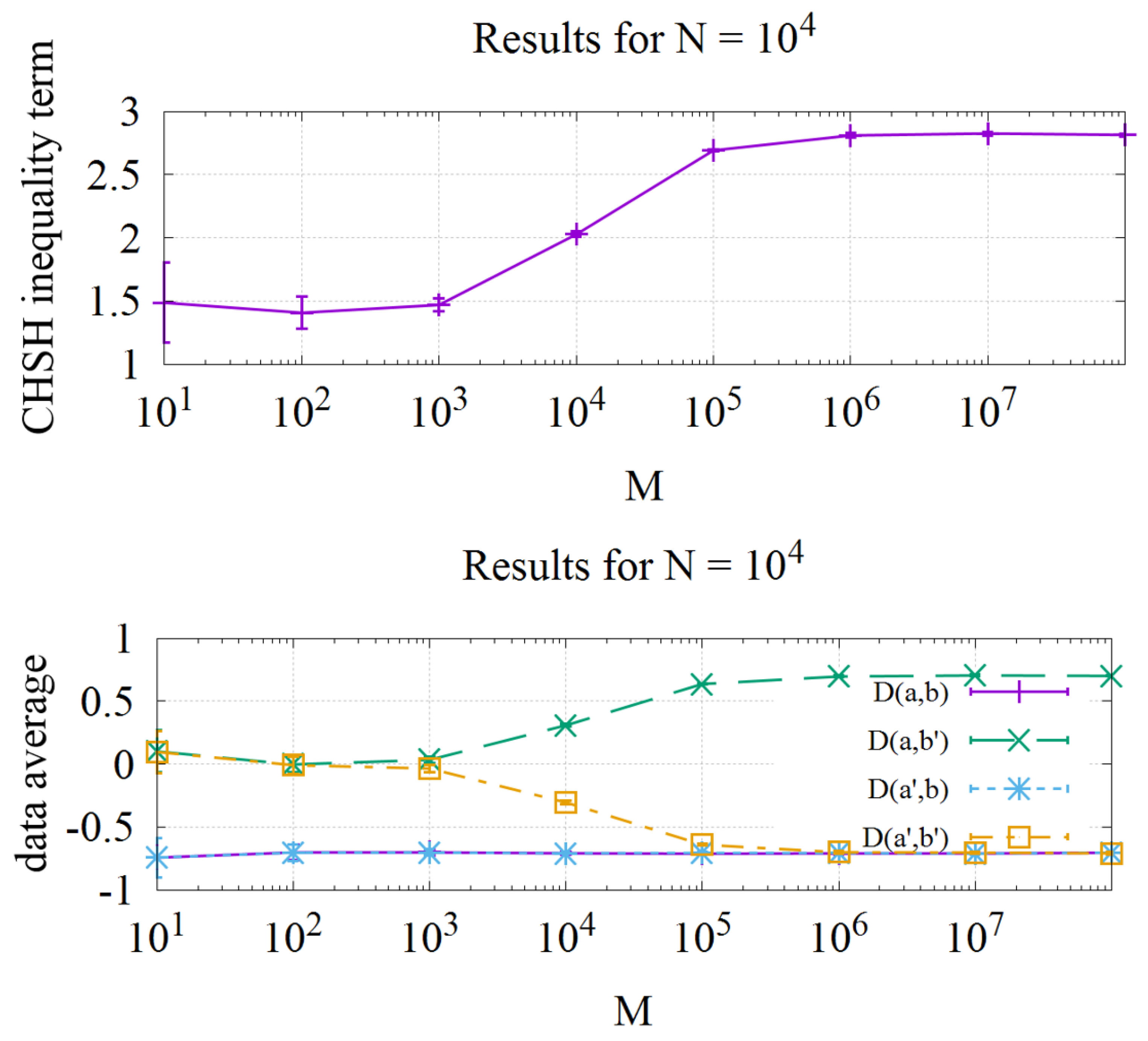
 M . The upper half of Figure 1 shows the mean values and standard deviations (error bars) of the CHSH-term. The lower half shows the corresponding mean of the averages D for given polarizer angle-pairs. We always have the marginal averages < A > 0 and < B > 0 for any polarizer angle; for example, we have for M = 10 7 and N = 10 4 values of < A > = 0.0014 ± 0.0029 and < B > = 0.0013 ± 0.0033 .
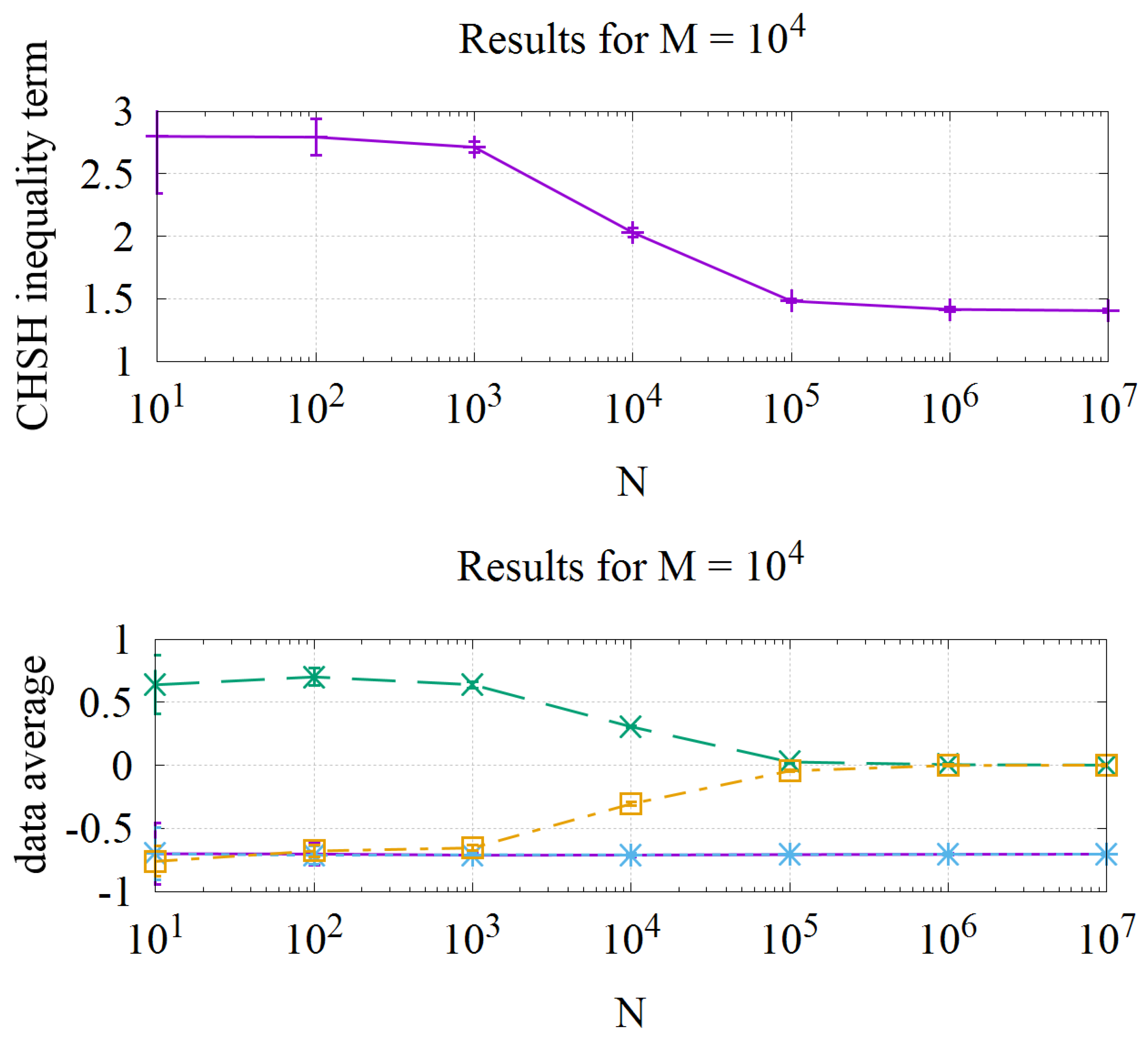
For the second series of MCCEs, we used M = 10 4 and varied the number of measurements from N = 10 by factors of 10 up to N = 10 3 · M = 10 7 . The upper half of Figure 2 shows the mean value and standard deviation of the CHSH-term of Equation (6) and in the lower half the averages D for a given polarizer angle-pair with the standard deviation given as error bars. The marginal averages are again about zero.
In both Monte Carlo series of computer experiments, two regimes can be distinguished: if the number M of different λ s values is significantly larger than the number of computer “measurements” N , then the averages follow the QM prediction and the CHSH-term is close to the quantum result of 2.82 and violates the CHSH inequality. If M is significantly smaller than N , then the CHSH inequality is fulfilled and the CHSH term of the four product averages A B differ from the QM prediction.
Thus, it appears to be entirely clear that what matters for violations of Bell–CHSH is the relation of the number N of model measurements to the number M of different model elements of physical reality λ i n . If M N , the Malus type law that we have imposed by using Equations (3) and (4) always wins and the Bell–CHSH inequalities are violated, while for M N the Bell–CHSH inequalities always win and the Malus-type law plays no significant role.
An interesting point has surfaced in the course of these investigations. The computer model is locally deterministic if the Malus law is implemented exactly the way we have described it above. Such implementation can certainly be made if we use four different pairs of computers at four different places, one computer pair for each pair of polarizer angles and each pair supplied by a different source of random numbers from the interval [−1, +1]. The Bell–CHSH inequalities lead to a nonlocal effect in this case. The averages that are obtained at the four different locations are not independent of each other. Thus, proofs of Bell–CHSH like those of Mermin unwittingly introduce a nonlocality, because they use a given number M of elements of physical reality that leads to a combinatorial symmetry, which we investigate next using our Monte Carlo simulations.

3.2. Role of Cyclicity, a Combinatorial Symmetry

The importance of Vorob’ev’s topological–combinatorial cyclicity [11] for the four CHSH-type experiments may be investigated by suppressing the combinatorial symmetry artificially in the MC computer experiments. It appears that Bell–CHSH have been dealing with a very subtle symmetry that may be broken for a variety of innocuous reasons because it does not necessarily correspond to a law of nature, although it was mistakenly assumed to follow exclusively from locality and determinism. However, the combinatorial symmetry occurs in the computer experiments if and only if the results A ( a , λ 1 n ) occurring for the polarizer angle-pair ( a ,   b ) corresponding to i = 1 are stored in the same array A a [ 1 ,   ,   M ] as the results A ( a , λ 2 n ) for the angle-pair ( a ,   b ) corresponding to i = 2 (similar arguments apply to the arrays A a , B b and B b ), which does not follow from the premises of locality and determinism. We have already seen in the previous section that these combinatorial symmetry requirements (used in all Bell–CHSH proofs) are true only for N M (in which case about all the λ i n can be suitable reordered) and are false for N M , because in this latter case, nearly all the λ i n are different and cannot be reordered. Bell–CHSH and all their followers did not notice the cardinality dependence of their inequality. They claimed their inequalities follow from their use of a local-deterministic model. We discuss their reasoning in the next section in detail. The combinatorial symmetry is made impossible by creating eight arrays, A a 1 , A a 2 , B b 1 , B b 3 , A a 3 , A a 4 and B b 2 , B b 4 (instead of four arrays A a , A a , B b and B b ) in which the respective function values A a ,   λ 1 n and A ( a ,   λ 2 n ) are stored in separate arrays A a 1 and A a 2 for polarizer setting pairs i = 1 and i = 2 (an analog separation of arrays is used for the other polarizer pairs by B b 1 , B b 3 , A a 3 , A a 4 and B b 2 , B b 4 ).
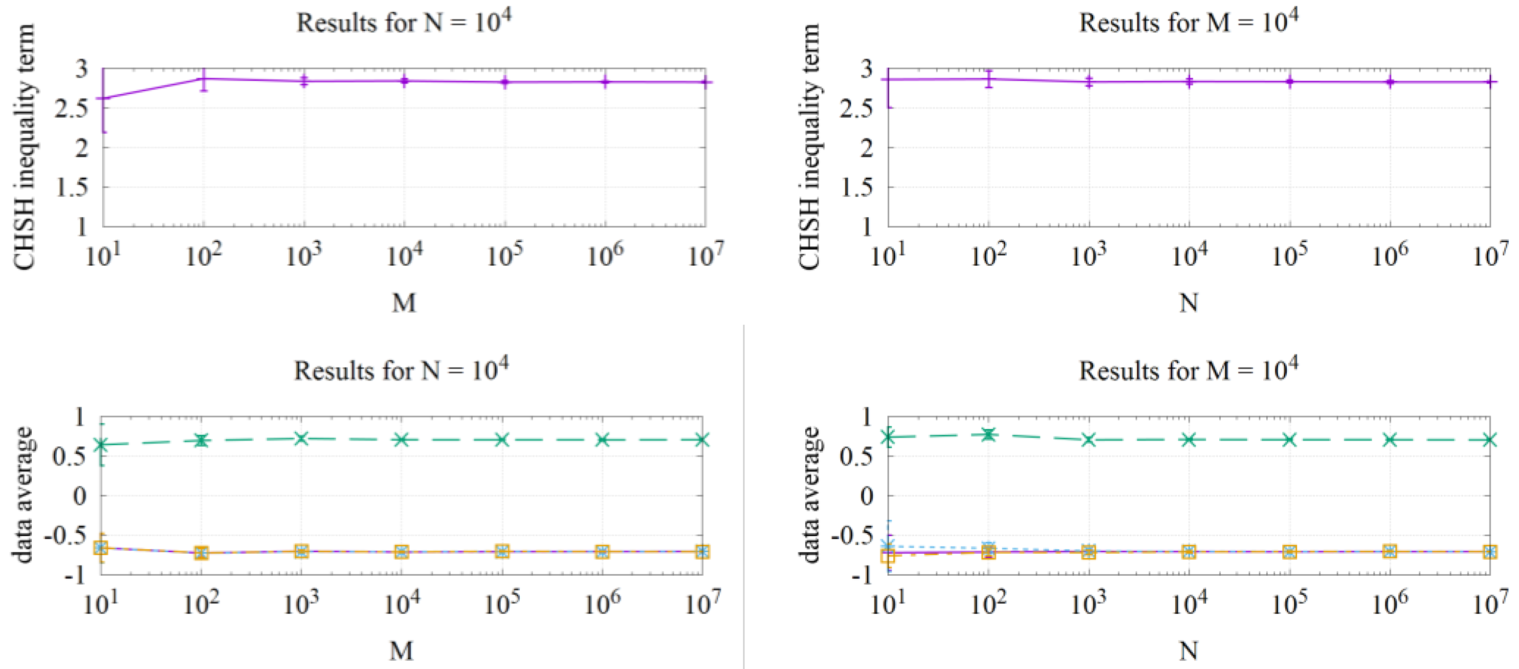
Figure 3 gives the CHSH-term (upper row) and the data averages (lower row) as function of M (left) and N (right) for the case of removed combinatorial symmetry. The CHSH-inequality is always violated and the data averages follow the QM predictions independent of the cardinalities of M versus N . The error bars are the standard deviations over 10 simulations of N experiments. These results demonstrate that combinatorial symmetry is mandatory to fulfill the CHSH-inequality.
In contrast, enforcing the combinatorial symmetry and always using the same λ i n (for i = 1 ,   2 ,   3 ,   4 ) must fulfill the CHSH inequality. Figure 4 gives the CHSH-term (left) and the data averages (right) with fixed N = 10 4 and increasing M from 10 to 107 using the standard deviations as error bar. As expected, the CHSH inequality is always fulfilled.
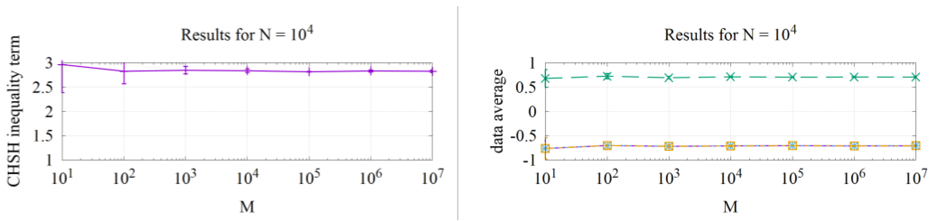
A further step is to use the same λ i n but suppress the combinatorial symmetry as described above by using separated arrays to memorize the settings of previous MC experiments. Figure 5 shows the CHSH term and the data averages for a simulation with identical λ i n and suppressed combinatorial symmetry. Without combinatorial symmetry, even using the same λ i n for the set of four CHSH experiments leads to a violation of the CHSH inequality and results that follow the predictions of quantum mechanics.

4. The CHSH–Aspect-Type Experiment and Computer Simulations

Having appreciated the above results, the question arises why the CHSH-type and Aspect-type experiments that are very similar in their nature to our computer model have received the interpretation with instantaneous influences at a distance and no possibility of explanation from local-deterministic models. If we assume a physically similar source in experiments that are performed for given polarizer angle pairs at four different locations, then the only difference to the Aspect-type experiments is that in the latter, the index i that denotes the polarizer angle pairs indicates different measurement times t i at the same locations. The measurements exhibit a time-like distance instead of a space-like distance. There should not be any difference between those cases, because Aspect has shown that rapid switching between the polarizer angles in the actual experiments does not influence the measurement outcomes.
The followers of Bell have, however, added another demand to the simulations that appears at first, again, very innocuous. They demand that the model experiments performed with computer pairs need to be able to come up with a result for any choice of polarizer angle-pairs and given λ i n . They make this demand because they believe that they are able to freely choose the polarizer angles in any moment of the actual experiments. There exists, however, a subtle difference between the actual experiments and any model experiments: in the actual experiments, nothing is known about the properties of the entangled photon pairs for any given measurement. We may have equal or not-equal outcomes of the actual experiments in the two stations, without knowing any probabilities for these outcomes. In the model experiments, the outcomes are determined by Equations (3) and (4) as soon as we have chosen the random λ i n out of the interval [ 1 λ i n + 1 ] . The demand is made by Bell’s followers that we must be able to simulate the possible outcomes for four polarizer angle-pairs and any given λ i n . This situation, however, corresponds to the enforced combinatorial symmetry, which always leads to the Bell–CHSH inequalities. One just cannot obtain four consistent statistical results of the Malus type in the presence of a combinatorial symmetry as shown clearly by our MC simulations.
Note that the experimenters in the actual experiments with photon pairs can certainly not guarantee that they measure exactly the same properties of any given photon pair with four different polarizer angle-pairs. They can perform only one measurement for any given entangled photon-pair. The cardinality of the set of all photon-pair properties is not known. It appears possible to restrict this cardinality by putting polarizers or other instrumentations right after the source. While the degree of restrictions of the cardinality by such methods is unclear, the literature does suggest that some such restrictions lead to Bell–CHSH, although no such actual measurements have been performed to the knowledge of the authors.

5. Conclusions

We have performed Monte Carlo simulations of CHSH-type experiments. Our computer model deviates from the Bell–CHSH models mainly through our use of the Fundamental Model of Probability theory combined with a Malus-type law for the correlations between the polarizations of the photon-pair measurements.
The use of the Fundamental Model permits different photon-pair properties for every single event of photon-pair emission. This factor is shown to be critical for the possibility of breaking the combinatorial symmetry of the Vorob’ev cyclicity and consequential violations of the Bell–CHSH inequalities. As soon as the Fundamental Model is used, the cardinality of the number of different photon-pair properties M as related to the cardinality of the number of measurements N becomes of critical importance and violations of Bell–CHSH are obtained in all cases of M N . We have shown in great detail that the reason for the validity of Bell–CHSH inequalities is a combinatorial symmetry that was originally discovered by Vorob’ev [11]. We have introduced and removed such combinatorial symmetry in our Monte Carlo simulations and have shown that, for all cases that we could consider, the presence of such a combinatorial symmetry leads to the Bell–CHSH inequalities, while the absence of the combinatorial symmetry (that depends on the relative cardinalities of N ,   M ) leads to violations and the quantum results, even if the model is local deterministic.
As we have shown, the presence of a combinatorial symmetry may be induced by very innocuous assumptions in addition to the assumption of local determinism. These additional assumptions have been made unwittingly by Bell and his followers, with a particular example presented by Mermin’s elegant proofs using M = 8 . Other authors have introduced combinatorial symmetry in other ways. Leggett [13], for example, has used counterfactual reasoning, assuming that, for a given photon pair property, he could have chosen all four CHSH polarizer-angle pairs. Our Monte Carlo model does not permit such a choice and we cannot see how one could demand from nature what is obviously not necessarily allowed in computer experiments. Our computer experiments certainly refute that Bell–CHSH might be seen as a proof of “impossibility”. Violations are possible in computer experiments.
These findings contradict the claim of the 2022 physics Nobel laureates that Einstein’s physics (particularly his elements of physical reality) must lead to Bell–CHSH-type inequalities, which, in turn, are in contradiction with prize-winning experiments and measurements. In contrast, we have found that models following the classical physics of Einstein and using his elements (often also characterized by “hidden variables”) may and even must (under certain conditions regarding the cardinalities of M and N ) lead to results that are close to the results of quantum mechanics and to the prize-winning measurements. Any interpretation that denies Einstein’s elements and supports instead instantaneous influences at a distance is, therefore, put into question. Thus, the first measurements of photon entanglement by Kocher and Commins [3] also appear in a new light.

Author Contributions

J.J. and K.H. have contributed equally to the conceptualization and methodology of the performed modeling and simulation of Einstein–Podolsky–Rosen experiments by using Monte Carlo methods. They both contributed equally to the Monte Carlo framework. All coding and computing was performed by Jakumeit. Analysis and consequential conclusions were derived by both J.J. and K.H., who also wrote the manuscript together and agreed upon it. All authors have read and agreed to the published version of the manuscript.

Funding

This research received no external funding.

Data Availability Statement

The original contributions presented in this study are included in the article. The raw data supporting the conclusions of this article will be made available by the authors on request.

Acknowledgments

We would like to thank Andrei Khrennikov and Bengt Nordén for helpful discussions.

Conflicts of Interest

The authors declare no conflicts of interest.

References

  1. Einstein, A.; Podolsky, B.; Rosen, N. Can quantum-mechanical description of physical reality be considered complete? Phys. Rev. 1935, 47, 777–780. [Google Scholar] [CrossRef]
  2. Aspect, A. Closing the door on Einstein and Bohr’s quantum debate. Physics 2015, 8, 123. [Google Scholar] [CrossRef]
  3. Kocher, C.A.; Commins, E.D. Polarization correlation of photons emitted in an atomic cascade. Phys. Rev. Lett. 1967, 18, 575–577. [Google Scholar] [CrossRef]
  4. Nordén, B. Entangled photons from single atoms and molecules. Chem. Phys. 2018, 507, 28–33. [Google Scholar] [CrossRef]
  5. Bell, J.S. On the einstein podolsky rosen paradox. Phys. Phys. Fiz. 1964, 1, 195. [Google Scholar] [CrossRef]
  6. Clauser, J.F.; Horne, M.A.; Shimony, A.; Holt, R.A. Proposed experiment to test local hidden-variable theories. Phys. Rev. Lett. 1969, 23, 880–884. [Google Scholar] [CrossRef]
  7. Hess, K. A Critical Review of Works Pertinent to the Einstein-Bohr Debate and Bell’s Theorem. Symmetry 2022, 14, 163. [Google Scholar] [CrossRef]
  8. De Baere, W. Significance of Bell’s inequality for hidden-variable theories. Lett. Nuovo Cimento 1984, 39, 234–238. [Google Scholar] [CrossRef]
  9. Williams, D. Weighing the Odds; Cambridge University Press: Cambridge, UK, 2001; pp. 44, 73, 110. [Google Scholar]
  10. Hess, K. Malus-law models for aspect-type experiments. J. Mod. Phys. 2023, 14, 1167–1176. [Google Scholar] [CrossRef]
  11. Vorob’ev, N.N. Consistent families of measures and their extensions. Theory Probab. Appl. 1962, 7, 147–163. [Google Scholar] [CrossRef]
  12. Mermin, N.D. Is the moon there when nobody looks? Reality and the quantum theory. Phys. Today 1985, 38, 38–47. [Google Scholar] [CrossRef]
  13. Leggett, A.J. The Problems of Physics; Oxford Academic: Oxford, UK, 2006; pp. 164–165. [Google Scholar]
Figure 1. (Upper half) mean value (standard deviation as error bar) of the CHSH-term as given in Equation (6) for N = 10 4 . (Lower half) averages D ( a ,   b ) in purple, D ( a ,   b ) in green, D a ,   b in blue and D ( a ,   b ) in yellow. The standard deviations are also indicated as error bars. The last data point on the right is for always new λ (approaching the limiting value of the Fundamental Model of Probability for M   ).
Symmetry 16 00255 g001
Figure 2. (Upper half) mean value (standard deviation as error bar) of the CHSH-term of the results with M = 10 4 . (Lower half) corresponding mean of the data averages (averages D ( a ,   b ) in purple, D ( a ,   b ) in green, D a ,   b in blue and D ( a ,   b ) in yellow, standard deviation as error bar).
Symmetry 16 00255 g002
Figure 3. (Upper row) mean value (standard deviation as error bar) of the CHSH-term of the results of first series with N kept constant on the left and the results of the second series with M constant on the right. (Lower row) corresponding mean of the data averages (standard deviation as error bar). As always, we have averages D ( a ,   b ) in purple, D ( a ,   b ) in green, D a ,   b in blue and D ( a ,   b ) in yellow.
Symmetry 16 00255 g003
Figure 4. CHSH-term (left) and the data averages (right) with fixed N = 10 4 and increasing M from 10 to 107 using the standard deviations as error bar for MCCEs with cyclicity and always using the same λ i n (for i = 1 ,   2 ,   3 ,   4 ) (averages D ( a ,   b ) in purple, D ( a ,   b ) in green, D a ,   b in blue and D ( a ,   b ) in yellow).
Symmetry 16 00255 g004
Figure 5. CHSH-term and the data averages for a simulation with identical λ i n and suppressed cyclicity. (averages D ( a ,   b ) in purple, D ( a ,   b ) in green, D a ,   b in blue and D ( a ,   b ) in yellow).
Symmetry 16 00255 g005
Disclaimer/Publisher’s Note: The statements, opinions and data contained in all publications are solely those of the individual author(s) and contributor(s) and not of MDPI and/or the editor(s). MDPI and/or the editor(s) disclaim responsibility for any injury to people or property resulting from any ideas, methods, instructions or products referred to in the content.

