Article

Comprehensive Sensitivity Analysis Framework for Transfer Learning Performance Assessment for Time Series Forecasting: Basic Concepts and Selected Case Studies †

by
Witesyavwirwa Vianney Kambale
1,2,
Mohamed Salem
1,
Taha Benarbia
3,
Fadi Al Machot
4 and
Kyandoghere Kyamakya
1,5,*
1
Institute for Smart Systems Technologies, Universitaet Klagenfurt, 9020 Klagenfurt, Austria
2
Faculty of Information and Communication Technology, Tshwane University of Technology, Private Bag x680, Pretoria 0001, South Africa
3
Institute of Maintenance and Industrial Security, University of Oran 2, Oran 31000, Algeria
4
Faculty of Science and Technology, Norwegian University of Life Sciences (NMBU), 1430 Ås, Norway
5
Faculté Polytechnique, Université de Kinshasa, Kinshasa XI P.O. Box 127, Democratic Republic of the Congo
*
Author to whom correspondence should be addressed.
This paper is an extended version of our paper published in the Circuits, Systems, Communications and Computers (CSCC-2023) Conference, Rhodes Island (Rodos Island), Greece.
Symmetry 2024, 16(2), 241; https://doi.org/10.3390/sym16020241
Submission received: 18 November 2023 / Revised: 2 February 2024 / Accepted: 14 February 2024 / Published: 16 February 2024

Abstract

:
Recently, transfer learning has gained popularity in the machine learning community. Transfer Learning (TL) has emerged as a promising paradigm that leverages knowledge learned from one or more related domains to improve prediction accuracy in a target domain with limited data. However, for time series forecasting (TSF) applications, transfer learning is relatively new. This paper addresses the need for empirical studies as identified in recent reviews advocating the need for practical guidelines for Transfer Learning approaches and method designs for time series forecasting. The main contribution of this paper is the suggestion of a comprehensive framework for Transfer Learning Sensitivity Analysis (SA) for time series forecasting. We achieve this by identifying various parameters seen from various angles of transfer learning applied to time series, aiming to uncover factors and insights that influence the performance of transfer learning in time series forecasting. Undoubtedly, symmetry appears to be a core aspect in the consideration of these factors and insights. A further contribution is the introduction of four TL performance metrics encompassed in our framework. These TL performance metrics provide insight into the extent of the transferability between the source and the target domains. Analyzing whether the benefits of transferred knowledge are equally or unequally accessible and applicable across different domains or tasks speaks to the requirement of symmetry or asymmetry in transfer learning. Moreover, these TL performance metrics inform on the possibility of the occurrence of negative transfers and also provide insight into the possible vulnerability of the network to catastrophic forgetting. Finally, we discuss a sensitivity analysis of an Ensemble TL technique use case (with Multilayer Perceptron models) as a proof of concept to validate the suggested framework. While the results from the experiments offer empirical insights into various parameters that impact the transfer learning gain, they also raise the question of network dimensioning requirements when designing, specifically, a neural network for transfer learning.

1. Introduction

1.1. Background and Motivation

The ability to predict future values based on historical data, known as time series forecasting, has become increasingly crucial in various fields, including finance, energy, healthcare, and transportation [1,2]. Precise predictions allow companies and policymakers to foresee trends, make informed decisions, and allocate resources efficiently. However, the intrinsic features of time series data, such as temporal dependencies, non-stationarity, and noise, render the task of forecasting time series a challenging issue within the realms of mathematics and machine learning. Fortunately, deep learning models have received significant focus in this domain and are praised for their capacity to capture the stochasticity and complexity present in time series data.
On another front, data limitations still pose significant challenges. Specifically, insufficient amounts of training data, scarce labeled data, and variations in data distributions across different domains are constant challenges in machine learning and deep learning. [3]. Transfer learning has emerged as an effective approach to tackle these issues by utilizing knowledge acquired from one or more related domains to enhance prediction accuracy in a target domain where data are scarce. The rationale for transfer learning lies in the idea that models can learn common patterns, trends, and underlying relationships from a source domain and transfer this knowledge to enhance performance in a target domain [3].
Conceptually, transfer learning involves the notions of a domain and a task [4]. A domain D consists of a feature space X and a marginal probability distribution P(X), where X = { x 1 ,   , x n } X and n is the number of feature vectors in X. X is the space of all the possible feature vectors, and X is a particular learning sample. So, generally, if two domains are different, they may, therefore, have different feature spaces or different marginal probability distributions. Also, given a specific domain D = { X , P ( X ) } , task T consists of a label space Y and a predictive function f ( · ) , denoted by T = { Y , f ( · ) } . The function f ( · ) is a predictive function, that is, it represents a mapping from the feature space to the label space. Consequently, it can be used to make predictions based on unseen data. Now, given a source domain D S and learning task T S , on the one hand, and a target domain D T and learning task T T , on the other hand, the goal of transfer learning is to improve the learning of the target predictive function f T ( · ) in D T using the knowledge in D S and T S , where D S D T or T S T T .
While transfer learning has been widely and effectively used in Computer Vision (CV) [5] and Natural Language Processing (NLP) [6], it is only recently that the use of transfer learning for time series data has gained momentum [7]. Although numerous research studies have successfully applied transfer learning for time series prediction in areas like finance and electricity, the sentiment of the research community on the topic is that more exploration into the theoretical foundations of transfer learning and time series analysis is still needed. For instance, the authors of [8] contend that empirical studies that can evaluate the benefits of different TL approaches with various types of time series data for various prediction problems are still to be performed.
Conducting their experiments in CV, Mensink et al. [9] note that existing systematic studies on Transfer Learning have been limited, and the circumstances in which developed TL techniques are expected to work, in most cases, are not fully understood. This cannot be more true for TL in time series forecasting, in which transfer learning is still in its infancy. Furthermore, the survey [10] highlights a shortage of empirical studies that thoroughly assess the advantages of various transfer learning methods across a range of time series data types for different prediction problems. Therefore, empirical studies are essential to developing guidelines for TL approaches and TL selection or method design that can be utilized by time series practitioners.
The primary contribution of this paper is the suggestion of a comprehensive framework for Transfer Learning Sensitivity Analysis for Time Series Forecasting. We achieve this by identifying various parameters seen from various angles of transfer learning applied to time series, aiming to uncover factors and insights that influence the performance of transfer learning in time series forecasting. A further contribution is the introduction of four TL performance metrics encompassed in our framework. These TL performance metrics provide insight into the extent of the transferability between the source and the target domains. Moreover, they inform on the possibility of the occurrence of negative transfers and also provide insight into the possible vulnerability of the network to catastrophic forgetting.
Furthermore, the concept of transfer learning, articulated through several dimensions and reflecting balance and equivalence in the transfer of knowledge from a source domain to a target domain, speaks to the idea of symmetry. Moreover, seen in the context of encapsulating the harmonious exchange of learned patterns, ensuring that the benefits of transferred knowledge are equally accessible and applicable across different domains or tasks, leads to the requirement of symmetry in transfer learning. In the case of transfer learning in time series forecasting, symmetry is to be regarded as a core requirement. For example, the balanced transfer of knowledge means that the knowledge gained from the source domain can be used effectively and efficiently in the target domain without any bias or loss of relevance. Thus, expressing symmetry in transfer learning involves ensuring a balanced, equitable, and harmonious application and impact of transferred knowledge across different domains and tasks.

1.2. Problem Statement and Research Questions

Comprehensive and sufficiently extensive SA-related experimental/simulative/conceptual studies are still/very much needed to provide insights into:
  • To what extent do specific contextual parameters impact the effectiveness of TL, in the context of time series forecasting tasks and endeavors;
  • How the TL performance evolves in view of variations of certain contextual parameters and dimensions related, amongst others, to machine learning (ML)/neural network (NN) model types, the configuration of the ML model, the difference in distribution or distance between the source and target domains, the size of the lag and horizons for TSF, etc.;
  • How to formulate recommendations on ML/NN model architectures and their subsequent TL-aware configurations and dimensioning in view of practical requirements with respect to low model complexity for better implementability on hardware platforms, etc.
Based on the above problem statement and the various TL for TSF shortcomings discussed in [10,11], we define the following research questions (RQs):
RQ1: How can one comprehensively assess the TL performance of a network in a given TL scenario (i.e., suggest a comprehensive TL performance analysis framework that is ML/NN model-independent)? We answer this question, first by conducting a brief critical state-of-the-art review related to TL performance metrics and pinpointing the gap in this regard. Second, we suggest and define novel TL performance metrics for our framework.
RQ2: What are the essential elements of a comprehensive TL-related Sensitivity Analysis framework, in the context of TSF, independently of a given ML/NN model? In other words, how can a comprehensive methodology for a TL sensitivity analysis for any ML/NN model be framed? We address this question by (1) surveying the TL techniques that are applicable to TSF; (2) discussing how far the TL performance analysis framework developed in RQ1 is applicable to all the identified TL techniques applicable to TSF; (3) providing a brief background and motivation for a comprehensive TL Sensitivity Analysis, first, in general, and second, specifically for TSF; also, we formulate a specification book for a comprehensive TL sensitivity analysis for TSF; (4) providing a critical literature review with respect to TL related-Sensitivity Analysis and identify the gap in this regard; and (5) conducting a thorough investigation all the relevant TSF-related TL Sensitivity Analysis contextual dimensions and parameters related to the ML/NN model, TSF Input/Output modeling, Source-Target Domain distribution and distance characteristics, TL technique, and Robustness to adversarial noise.
RQ3: How can a comprehensive TL Sensitivity Analysis framework be formulated, taking an ensemble TL for TSF as a use case and proof of concept? To answer this question, first, we briefly discuss ensemble learning techniques. Then, we discuss dimensions and parameters that are to be considered in a comprehensive Ensemble TL Sensitivity Analysis. Finally, we present the selected dimensions and parameters that we consider for implementation as a proof of concept.
RQ4: To what extent do the dimensions and parameters selected in the Sensitivity Analysis framework (RQ3) impact the transfer learning performance? To answer this question, we present the results of the experiments by discussing the underlying insights with respect to the transfer learning process, thereby demonstrating the effectiveness and feasibility of this methodology in practice.
The remainder of the paper is structured as follows: Section 2 introduces a Comprehensive Transfer Learning Performance Analysis Framework. Section 3 discusses the Essential Elements of Comprehensive TL-Related Sensitivity Analysis in the Context of Time Series Forecasting. Section 4 offers a brief overview of ensemble learning techniques, while Section 5 implements the Ensemble Transfer Learning Sensitivity Analysis as a use case. Finally, Section 6 provides concluding remarks and directions for future study.

2. A Comprehension Transfer Learning Performance Analysis Framework (RQ1)

In this section, we present a comprehensive framework for analyzing transfer learning performance, offering a systematic approach to evaluating the extent of transferability, adaptability, and effectiveness across diverse domains. We start by surveying the literature about transfer learning performance metrics. We then introduce our framework, which encompasses a range of TL performance metrics, allowing researchers and practitioners to gain deeper insights into the transfer learning process and make informed decisions to optimize performance for specific tasks and domains.

2.1. Critical State-of-the-Art Review of TL Performance Metrics

Transfer learning, a prominent machine learning paradigm, has revolutionized several domains by enabling models to use knowledge acquired on one task to improve performance on another task. However, the effectiveness of transfer learning models depends on the careful selection and evaluation of performance measures. In this section, we are conducting a brief state-of-the-art review of the key metrics used to assess the performance of transfer learning models, highlighting their strengths, limitations, and recent developments.
The authors of [12] undertook a task to study and compare the network performance of five selected pre-trained models based on transfer learning. The authors note an important challenge with conducting transfer learning: certain layers of a pre-trained model require retraining, whereas others must be left untouched to ensure effective adaptation to a new task. However, typical issues encountered have to do with the selection of the layers that must be enabled for training and the layers that must be frozen. Eventually, these concerns, together with setting hyperparameter values, will have a substantial effect on the training capabilities and the extent of the transfer learning performance. The paper does not suggest metrics to assess the performance of the transfer learning process. But to reach their aim, they simply compare the accuracy of the five selected pre-trained models. Wang et al. [13], starting from a simple and intuitive premise about TL that learning a new concept is easier if one has previously learned one or more similar concepts, propose a TL performance metric that they call the performance gap. They define the performance gap as a measure of the discrepancy between the source and target domains, regarded as an algorithm-dependent regularizer that controls the model complexity to be upper-bounded. However, even though the performance gap is both data- and algorithm-dependent, the metric is considered crucial for a more informative and finer generalization bound. The study by Weiss and Khoshgoftaar [14] provides a discussion of the relative performance analysis of state-of-the-art transfer learning algorithms and traditional machine learning algorithms. Their analysis addresses the question of whether the area under the curve (AUC) performance is predictive of classification accuracy in a transfer learning environment, where there is no labeled target data to perform validation methods.
The study in [15] has conducted a survey on transfer learning. Their surveyed works demonstrate how transfer learning has been applied to many real-world applications. Next are some of the applications and the performance metrics used for transfer learning. For Imagine classification, multi-language text document classification, multi-language text sentiment classification, and document text classification, classification accuracy is measured as the performance metric. For word classification, the F1 score is measured as the performance metric. For object category recognition, the area under the curve (AUC) is measured as the performance metric. Moreover, the average precision is measured as the performance metric for the object image classification application.
When it comes to regression tasks in transfer learning, mean squared error, root mean squared error, or mean absolute error are the preferred metrics to quantify the difference between the TL model’s outputs and the actual values [16,17].
A study posing a question similar to the one we have presented in this study is referenced in [18]. We agree with the fundamental premise that assessing transferability is crucial for a transfer learning task. This refers to providing insight into when transfer learning may be effective and the extent to which it can work. Given a metric capable of efficiently and accurately measuring transferability across arbitrary tasks, the problem of learning about task transfers simplifies largely to search procedures about potential transfer sources and targets as quantified by the metric. Traditionally, transferability has been measured using the model’s accuracy, as stated in the cases above. We equally have studies that have focused on task relatedness [19] and domain similarity and dissimilarity [20,21], as will be discussed in Section 3.5.3. However, they cannot directly explain task transfer performance, and the H-score proposed in [18] only estimates the performance of transferred representations from one task to another in classification problems. That is why we are proposing our four TL metrics. Our proposition necessitates that we briefly discuss the issues of negative transfer and catastrophic forgetting. One conclusion from [14] is that analyzing the relative performance of TL algorithms across a wide range of distortion profiles should be considered an area for future research. Negative transfer occurs when the source domain data and tasks contribute to lower learning performance in the target domain. Despite the fact that the prevention of negative transfer is a very important issue, little research has been published on this topic [19].

2.2. Negative Transfer and Catastrophic Forgetting in Transfer Learning

Though Transfer learning comes with numerous promises, such as an effective way to train models quickly and efficiently, especially for tasks and domains where there is a limited amount of data available [15], the effectiveness of transfer learning is not always guaranteed [22]. Two of the potential dilemmas faced by transfer learning are: negative transfer and catastrophic forgetting.
Negative transfer poses a limit to the power of transfer learning [22]. As put in [4], when designing transfer learning, one has to be sure of what to transfer, how to transfer, and when to transfer. What to transfer refers to determining which part of knowledge can be transferred across domains or tasks. Certain knowledge can be specific to certain domains or tasks, while other knowledge can be shared across multiple domains, potentially enhancing performance in the target domain or task. After determining what knowledge can be transferred, learning algorithms must be designed to transfer the knowledge, which corresponds to answering the question of how to transfer. Next, knowing when to transfer refers to determining situations in which knowledge should be transferred, implying knowing in which situations knowledge should not be transferred. In some cases, if the source domain and target domain are unrelated, a brute-force transfer approach might not succeed. In the worst scenario, this could even impair the learning performance in the target domain, a situation commonly known as negative transfer. So, in short, negative transfer occurs when the performance in the target domain deteriorates instead of improving during the transfer learning. Nevertheless, how to avoid and prevent negative transfers remains an important open issue that has yet to be fully addressed.
On the other side, catastrophic forgetting is another threat. After a network has been trained for a particular task, it cannot easily be trained to do new tasks. Typical deep neural networks tend to catastrophically forget previous tasks when new ones are introduced [23]. Catastrophic forgetting in neural networks occurs because of the stability-plasticity dilemma [24]. Normally, the network requires sufficient plasticity to learn new tasks, but significant changes in weights can lead to forgetting by disrupting previously learned representations. Maintaining the stability of the network’s weights protects against forgetting previously learned tasks, yet excessive stability hampers the model’s ability to learn new tasks. Networks that are designed to assimilate new information gradually, similar to the way humans accumulate new memories over time, will prove more efficient than completely retraining the model every time there is a need to learn a new task [23].
In short, catastrophic forgetting is the phenomenon where an artificial neural network abruptly forgets previously acquired information when it starts to learn new information. Negative transfer, on the other hand, happens when the performance in the target domain gets worse rather than better through the process of transfer learning [25]. Multiple factors contribute to these challenges, including the disparity between the source and target domains, the design of the transfer learning algorithm, and the quality of the source and target data.
So, it becomes imperative to devise ways that can, first, quantify the extent to which transfer learning is adversely affected by both negative transfer and catastrophic forgetting and, eventually, address these dilemmas. The scope of this study is focused on the former task. Readers interested in the development of the latter task can visit [23], suggesting methods to alleviate catastrophic forgetting in image data and [26] in time series data. The study in [27] also suggests ways of handling negative transfer, though the survey in [28], which is a decade-long survey of transfer learning, acknowledges that negative transfer is still an open challenge in transfer learning. However, the objective of this study is to suggest metrics that can provide insight into the occurrence of these phenomena during the transfer learning process. To this aim, transfer learning performance metrics are presented shortly.

2.3. Definition and Justification of Normalized Performance Metrics and Performance Assessment Scenarios

A variety of evaluation metrics are used in time series forecasting. Among these are the R-squared, the Mean Squared Error (MSE) and its variants such as the Root Mean Squared Error (RSME), the Mean Absolute Error (MAE), and its variants such as the Mean Absolute Percentage Error (MAPE), etc. However, we introduce a unified performance metric that encapsulates the combined information about RMSE and MAE. We denote this metric as the ePerfi metric (error performance), which we can define as
e P e r f i = 1 2 ( N R M S E i 2 + N M A E i 2 )
where NRMSE is the normalized RMSE, NMAE is the normalized MAE, and i   determines which error performance metric is calculated.
The NRMSE and NMAE are defined as follows:
N R M S E = R M S E y m a x y m i n
and
N M A E = M A E y m a x y m i n
where y m a x y m i n is the range of the (test) dataset. It can be noted that e P e r f i is computed as a quadratic mean of the NRMSE and the NMAE. This has been carefully thought through because of the robustness of the results that it can provide. The quadratic mean is a versatile mathematical concept that has useful properties for quantifying the magnitude and variability of the considered values and for analyzing data in a variety of contexts. It has the benefit of being less sensitive to outliers compared to other measures of central tendency.
Next, to establish a framework for the study, we define different performance assessment scenarios. These performance assessment scenarios are distinguished by whether the dataset that is used for training or testing, is taken from the source domain (training data 1 and test data 1) or the target domain (training data 2 and test data 2). Figure 1 and Table 1 offer more insights into understanding these performance assessment scenarios.
Thus, five basic error performance metrics, e P e r f i , are defined for five performance analysis scenarios. These error performance metrics can also be referred to as neural network’s performance metrics, as they assess the performance of neural networks set up in specific configurations.
To this end, we define three configurations (or states) of models: Model-1, Model-2A, and Model-2B; and in the experiments that will be carried out, all three models are of the same type. We consider them to be MLPs. Details about these models and the setup for the five performance analysis scenarios are provided in Figure 1.
Let us consider the two domains: the source domain and the target domain. The training data and test data of the source dataset are represented by Training Data 1 and Test data 1, respectively. And the training data and test data of the target dataset are represented by Training Data 2 and Test data 2, respectively. As for the models, Model-1 is considered the source model. But for the target model, we present two nuances: Model-2A and Model-2B. Model-2A presents a target model that results from the source model, Model-1, but that is fine-tuned by the target data. In other words, Model-2A is equivalent to a pre-trained Model-1, but with the difference that Model-2A is (or will be) fine-tuned by the target dataset before conducting the forecasting task. On the other hand, Model-2B, the second nuance of the target model, is a brand-new model that will be trained from scratch by the target dataset. That is, it has no pre-training configuration (condition).
Hence the definition of the following five performance analysis scenarios:
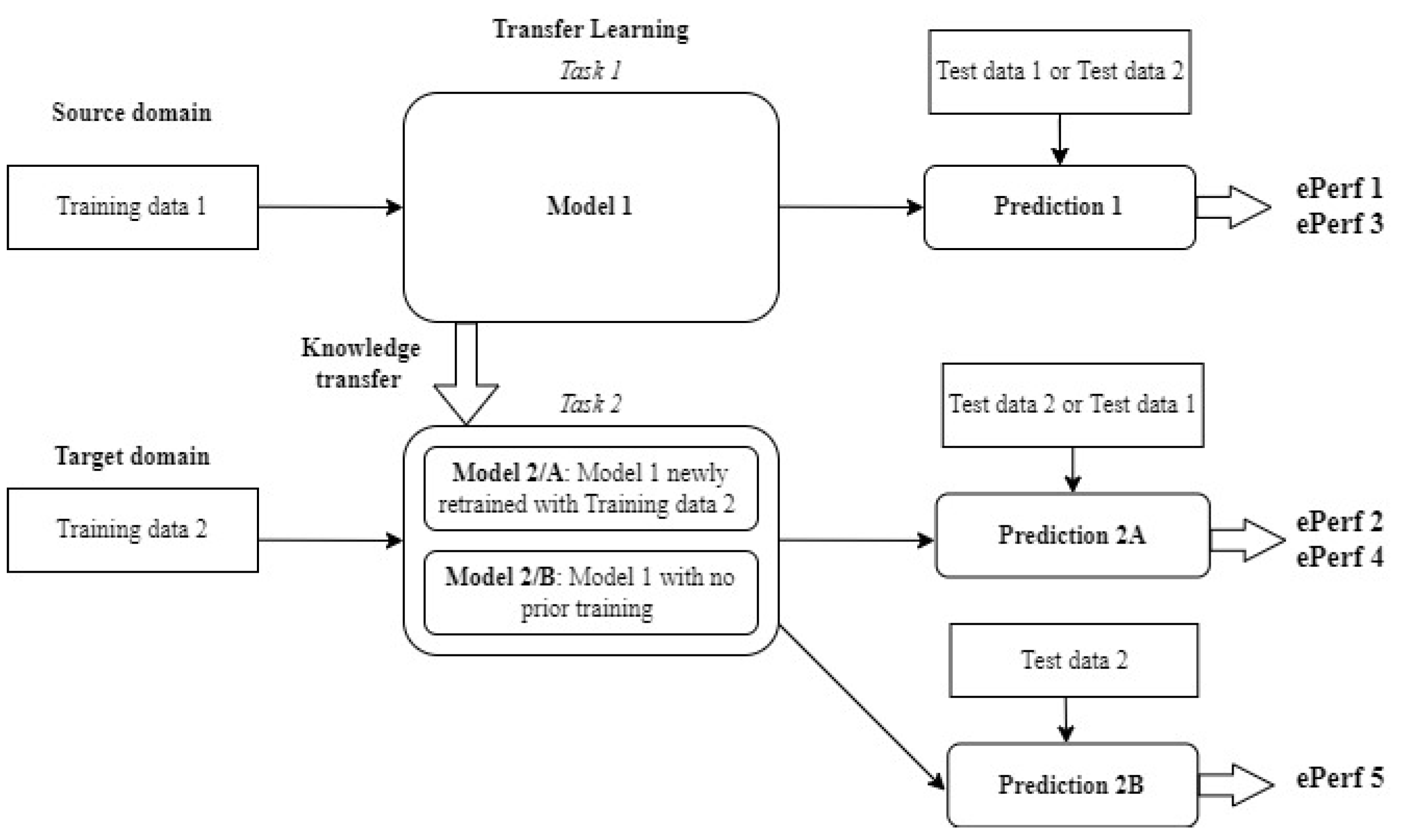
  • Performance analysis scenario 1: In this scenario, Training Data 1 is used to train Model-1, and Test data 1 is used to make predictions with Model-1. The resulting performance of this scenario is termed e P e r f 1 .
  • Performance analysis scenario 2: In this scenario, Training Data 2 is used to fine-tune, or to continue the training of, Model-1, which then becomes Model-2A. Then, Test data 2 is used to make predictions with Model-2A. The resulting performance of this scenario is termed e P e r f 2 .
  • Performance analysis scenario 3: The only action in this scenario is Test data 2, which is used to make predictions with Model-1, which was trained in scenario 1. The resulting performance of this scenario is called e P e r f 3 .
  • Performance analysis scenario 4: The only action in this scenario is that Test data 1 is used to make predictions with Model-2A, which was trained in scenario 2. The resulting performance of this scenario is called e P e r f 4 .
  • Performance analysis scenario 5: In this scenario, Training Data 2 is used to train Model-2B, and Test data 2 is used to make predictions with Model-2B. The resulting performance of this scenario is termed e P e r f 5 .
In short, for scenario 1, the training of the source model is performed by the source data, and the prediction is conducted by the source data using the source model. In scenario 3, no training is carried out. Simply put, the target data are used to make predictions with the source model. For scenario 2, target data are used to fine-tune or continue training the source model, which then becomes the first version of the target model. Then the target data are used to perform predictions with this version of the target model. In scenario 4, no training is carried out. Simply put, the source data are used to make predictions with the version of the target model constituted in scenario 2. And in scenario 5, the target data are used to train another version of the target model, a brand new model that has not undergone any prior training. Then, the target data are used to make predictions with this model.
The aim of these experiments is to produce the following five error performance metrics: e P e r f 1 , e P e r f 2 , e P e r f 3 , e P e r f 4 and e P e r f 5 , which are essential in defining the Transfer Learning performance metrics in the next section.

2.4. Definition and Justification of Comprehensive TL Performance Metrics

To gain insight into the level of transferability, we define the following novel transfer learning performance metrics: (a) TL gain (TLG), (b) TL forgetting ratio (TLFR), (c) reference generalization ratio (RGR), and (d) TL generalization gain (TLGG).
The transfer learning gain (TLG) is defined as follows:
T L G = e P e r f 5 e P e r f 2
It provides insight into the extent to which transfer learning occurred. When T L G is greater than 1 ( T L G > 1 ), it shows a positive TL impact compared to a case without prior training of the model used. When T L G is less than 1 ( T L G < 1 ), it shows an absolute negative transfer. When T L G = 1 , it shows a zero transfer situation.
The TL forgetting ratio (TLFR) is defined as follows:
T L F R = e P e r f 1 e P e r f 4
If the model is good at remembering, TLFR should be 1 or higher. In the case of TLFR < 1, we have a case of forgetting, and we speak of catastrophic forgetting when TLFR is significantly smaller than 1 (TLFR   1 ).
The TL generalization gain (TLGG) is defined as follows:
T L G G = e P e r f 3 e P e r f 2
It indicates how much gain we have gotten from the transfer learning compared to a simple use of Model 1 in the target domain without new retraining. TLGG is normally expected to be higher than 1 ( T L G G > 1 ). Any situation with TLGG < 1 indicates a negative TL-related generalization situation.
The reference generalization ratio (RGR) is defined as follows:
R G R = e P e r f 1 e P e r f 3
It tests the generalization capability of the source model. If the R G R is close to 1 ( R G R   1 ), that means the source model is good at generalization in the target domain. When R G R   1 , it means the source model is not good at generalization.
The set of these four novel metrics proposed above appears to be simple yet highly intuitive because they can be used to comprehensively assess the efficiency of transfer learning for a specific neural network architecture. They offer valuable insights into two types of negative transfer (absolute and generalization-related) as well as issues pertaining to eventual catastrophic forgetting that may occur during the transfer learning process.

3. Essential Elements of a Comprehensive TL-Related Sensitivity Analysis in the Context of Time Series Forecasting (RQ2)

In this section, we intend to comprehensively survey all the elements and parameters that can be useful in a TL sensitivity analysis. We do so by identifying the various dimensions and parameters seen from various angles of transfer learning applied to time series, aiming to uncover factors and insights that can influence the performance of transfer learning in time series forecasting. However, we start by surveying the TL techniques applicable to time series forecasting. We then discuss how far the developed TL performance analysis framework can be applicable to the surveyed TL techniques. Next, we provide a background and motivation for a comprehensive TL Sensitivity Analysis. We will finally perform a critical literature review of Sensitivity Analysis related to Transfer Learning before identifying all the aforementioned relevant contextual elements and parameters.

3.1. A Brief Survey of TL Techniques for TSF

When surveying the topic of TL techniques, it is noted that there are slight variations in the way diverse authors have previously categorized transfer learning methods. These categorizations result from using either the feature space or the task and domains as distinguishing criteria [29]. For example, Pan and Yang [4] categorize transfer learning methods based on differences in task and domain. They presented the following categories: inductive transfer learning, transductive transfer learning, and unsupervised transfer learning. In inductive transfer learning, the target task is different from the source task, regardless of whether the source and target domains are identical or not. In transductive transfer learning, the source and target tasks are the same, while the source and target domains differ. Finally, in unsupervised transfer learning, similar to inductive transfer learning, the target task is different from but related to the source task.
Unlike Pan et al., Weiss et al. [15] categorize transfer learning methods using the feature space as a criterion. They suggest two categories: homogeneous transfer learning solutions and heterogeneous transfer learning solutions. This categorization is based on the similarity between the source and target domains. Homogeneous transfer learning solutions are used when the domains are of the same feature space and the feature spaces of the data in the source and target domains are represented by the same attributes and labels while the space itself is of the same dimension. On the other hand, heterogeneous transfer learning solutions are used when the domains have different feature spaces, and the feature spaces between the source and target are nonequivalent and are generally non-overlapping. In this case, the source and target domains may share no features and/or labels, while the dimensions of the feature spaces may differ as well. It follows that heterogeneous transfer learning solutions are regarded as more complicated than homogeneous transfer learning solutions. This is because they require feature-space adaptation.
However, for the purpose of the subject of discussion in this study, we consider rather the categorization by Weber et al. [10]. This is a categorization that is specifically tailored for time series data (see Figure 2 and Table 2).

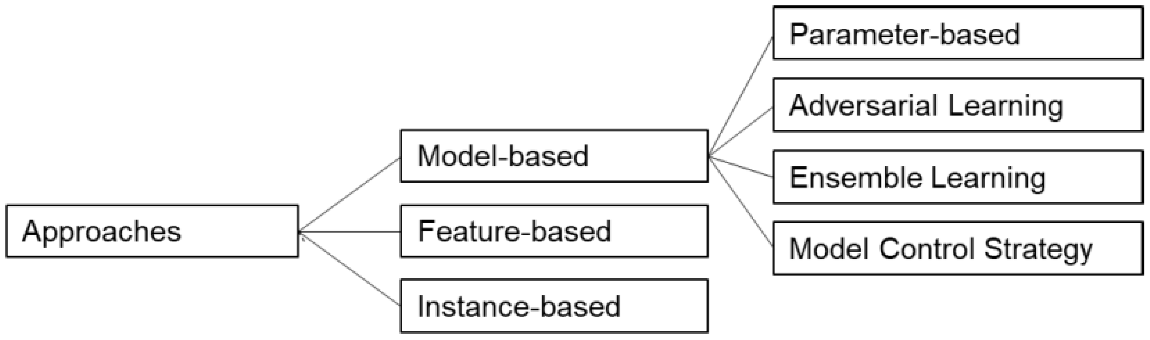
3.1.1. Model-Based Transfer Learning

This is the most common type of transfer learning, and it is the most widely used in time series. The approach focuses on transferring the model or parts of the model trained in the source domain to the target domain. The most common type of model-based transfer learning involves parameter transfer, where the parameters of a model that was pre-trained in the source domain are used to initialize the model in the target domain. For a neural network model, this encompasses the trained weights and biases.
There are two primary approaches based on parameter transfer, referred to as pre-training and fine-tuning and partial freezing. Apart from these two main approaches, we can identify additional alternative approaches, such as architecture modification, adversarial learning, ensemble-based transfer, and the use of an objective function specifically aimed at facilitating knowledge transfer.
  • Pre-training and fine-tuning approach: for the pre-training and fine-tuning approach, parameters from a model pre-trained on source data are either fully or partly employed to initialize a target model. This strategy aims to accelerate convergence during target training and enhance prediction accuracy and robustness. However, in many cases, all model parameters are reused for target training. A different but commonly used method involves transferring all weights to the target model except for the output layer, which is usually randomly initialized. Task adaptation is another aspect of fine-tuning [30]. Task adaptation, as a subcategory of transfer learning, involves adapting a pre-trained model to a new task that is related to the original task. The goal of task adaptation remains to improve the performance of the pre-trained model on the new task by leveraging the knowledge learned from the original task.
  • Partial freezing:partial freezing is a special case of fine-tuning, which is also frequently used in transfer learning for time series. Used particularly for neural network-based transfer, only selected parts of the model are retrained instead of retraining the whole model during a fine-tuning procedure. The parameters of the frozen layers are taken from the source model. The other layers to be fine-tuned are either initialized with source parameters or trained from scratch. As you survey the literature, one finds that it is mostly the output layer that is retrained, while the rest of the network is used as a fixed feature extractor based on the source data [31,32]. However, other studies have tried different numbers of frozen layers and different combinations of frozen and trainable layers [33,34].
  • Architecture modification: for the transfer learning process, some studies [35,36] have endeavored the architecture modification of the model used during source pre-training for subsequently being fine-tuned in the target domain. For example, modifications might entail either removing or incorporating certain layers in a deep learning model architecture. However, an intuitive approach can involve adding adaptation layers on top of the network that can only be trained with target data [35]. Moreover, for adaptation to a certain problem at hand, layers may also be added inside the existing layers of the source model [36].
  • Domain-adversarial learning: this is another approach to transfer learning that can be used to adapt a model from one domain (the source domain) to another domain (the target domain) where the data distributions are different. Influenced by the generative adversarial network (GAN) [37] concept and borrowing the notion of incorporating two adversarial components within a deep neural network that engage in a zero-sum game to optimize each other, this approach has been gaining interest [38,39,40]. As shown in Figure 3, a deep adversarial neural network (DANN) comprises three elements: a feature encoder, a predictor, and a domain discriminator. The feature encoder is made of several layers that transform the data into a new feature representation, whereas the predictor carries out the prediction task based on the obtained features. Moreover, the domain discriminator, which is a binary classifier, utilizes the same features to predict the domain from which an input sample is drawn.
In contrast to the TL approaches mentioned earlier, the operation of adversarial-based transfer is not divided into two stages: pre-training and adaptation. Instead, models are trained concurrently on both source and target data, which is then referred to as joint training. The predictor is trained using conventional supervised backpropagation, using the available label information from any of the two domains. Simultaneously, the adversarial objective is to generate domain-invariant features f so that, based on f, no distinction between the target and the source domain can be made. This aim is reached by calculating an additional domain discrimination loss, and linking the domain discriminator through a gradient reversal layer (GRL) that negates the gradient during backpropagation. This process is depicted in Figure 3.
  • Dedicated model objective: the concept underlying dedicated model objective is that, like in domain adversarial learning and unlike in model retraining, model objective functions, especially those dedicated to TL, allow using source and target data within a single training phase. Some studies that have investigated and applied this concept include [41,42,43].
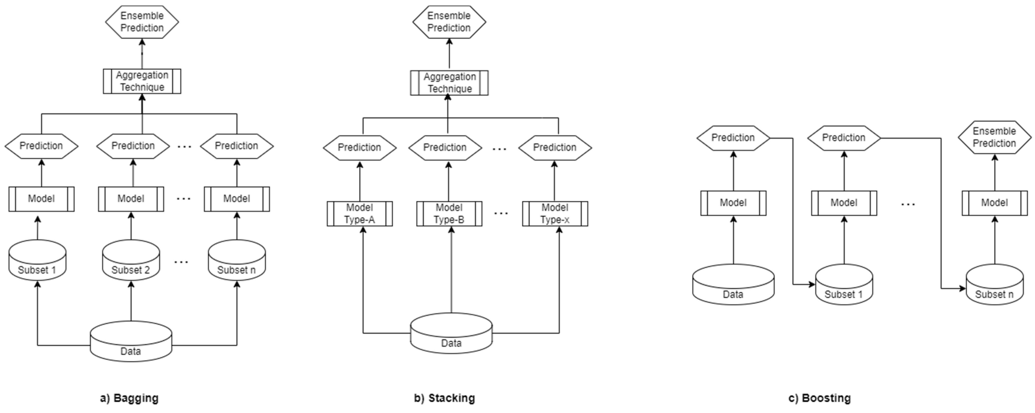
  • Ensemble-based transfer learning: this is a TL approach that exploits the concept of ensemble learning. Ensemble learning involves the combination of multiple base learners, where each one is trained independently on a subset of the available data. Generally, the objective of ensemble learning is to lower generalization errors. There are various configurations of ensemble techniques, but the major ones are bagging, boosting, and stacking techniques. All these techniques are being used for transfer learning with time series. The reader may be interested in looking at [44,45,46]. By the way, the use case chosen for implementation in this study is an ensemble technique (see Section 5).

3.1.2. Feature-Based Transfer Learning

The chief aim of feature-based transfer learning is to reduce the discrepancy between the feature spaces in the target and source domains. Hence, in feature-based transfer learning, the original features are transformed into a new feature space that is more suitable for the target task [10]. The goals of constructing a new feature representation are to reduce the difference between the marginal and conditional distributions, maintain the characteristics or underlying structures of the data, and establish a correspondence between features. For instance, let us consider a scenario of a cross-domain text classification problem [3]. The objective in this case is to build a target classifier using labeled text data from a similar domain. A practical approach is to identify common latent features via feature transformation and utilize them as a means for knowledge transfer.
The operations of feature transformation can be divided into three types, that is, feature augmentation [47], feature reduction (or feature selection) [48], and feature alignment [49]. The feature augmentation type of transfer learning involves adding new features to the existing feature space to improve the performance of the model on the target task. Feature augmentation can be performed by concatenating the original features with new features or by generating new features using techniques such as data augmentation. On the other hand, the feature reduction type of transfer learning involves reducing the dimensionality of the original feature space to improve the performance of the model on the target task. Feature reduction can be performed by techniques such as principal component analysis (PCA) or autoencoders. Finally, the feature alignment type of transfer learning involves aligning the feature spaces of the source and target domains to reduce the distribution differences between them. Feature alignment can be performed using techniques such as domain adaptation or adversarial training.
Nevertheless, Webber et al. [10] point out a nuance that is worth noting: the differentiation between ordinary feature transformation approaches and feature learning. They noted that in feature learning, a neural network encoder is learned with the goal of encoding data into a more useful feature space. In contrast to model-based techniques, in this method, the feature learning network is a separate model dedicated solely to transfer learning purposes. It can be combined with any distinct predictive model. Hence, the suggested grouping of feature-based transfer learning methods into methods that do not utilize a neural network, methods that are based on autoencoders [50], and methods based on a neural network that are not autoencoders [51] (see Table 3).

3.1.3. Instance-Based Transfer Learning

Instance-based transfer learning involves re-weighting the instances of the source domain to improve the performance of the model on the target domain. In instance-based transfer learning, the model is trained on the source domain, and then the weights of the instances are adjusted to minimize the difference between the source and target domains. This approach is useful when the source and target domains have different marginal distributions, but the conditional distributions are similar [52].
Instance-based transfer learning can be seen as a form of domain adaptation, where the goal is to adapt the source domain to the target domain by adjusting the weights of the instances. This approach is particularly useful when the target domain has limited labeled data, as it allows the model to leverage the labeled data from the source domain to improve the performance on the target domain [53].
For the purpose of time series, the subject at hand in this study, the term instance denotes an individual time series contained in a time series dataset. The study in [46] discusses two types of Instance-based transfer learning: Instance Selection and Symbolic Aggregation Approximation. In the Instance Selection method, a useful subset of instances from the source domain that are most relevant to the target domain is selected to train the target model [54]. Most selection methods take into account the similarity between source instances and the time series found in the target dataset. However, for Symbolic Aggregation Approximation methods, symbolic representations of the subset of instances from the source domain can be generated. For example, the study referenced in [55] employs the symbolic aggregation approximation (SAX) method to represent time series data, converting each time series into a word-like format. Such word representations can be compiled into a bag of words and, in this way, form a subset of the input data. The authors, subsequently, construct bags of words for different subjects. Transfer learning is carried out by collecting a bag of common words, where commonness is measured by the relative term frequency.

3.1.4. Hybrid Approaches

The literature also presents hybrid approaches. For instance, the study in [8] proposes a training strategy for time series transfer learning with two source datasets. First, a source model is trained with data from the first source data. Subsequently, the new source model is fully fine-tuned using the target data in the target domain. This is a hybrid case combining Freezing and Full Fine-Tuning. Additionally, hybrid approaches may be constructed with ensemble learning by combining them with other approaches such as pre-training and fine-tuning and others, as discussed in [56,57,58]. Further hybrid approaches can be found in Table 3.

3.2. How Far Is the Developed TL Performance Analysis Framework Applicable to All the TSF TL Techniques

The framework developed in Section 3.1 has presented metrics that can be used to evaluate the extent of transfer learning. Each TL metric sheds light on a crucial aspect of transfer learning. First, it indicates the potential gain that is achievable. Second, it provides insights into the occurrence, or lack thereof, of negative transfer. Lastly, it quantifies the risk of catastrophic forgetting in the network during the transfer learning process.
For the different transfer learning techniques surveyed applicable to time series forecasting, the network has been identified as either a neural network or a non-neural network (see Table 3).
Also, talking about the types of tasks identified for the time series data, the tasks can be regression, classification, or clustering. It can be noted that the suggested TL metrics were designed with a regression task in mind, where the error performance has been constructed using NMAE and NRMSE. This can lead us to conclude that these metrics, for now, are applicable to the regression forecasting task. However, the classification task’s version of the performance metrics can be designed. These will have to follow the logic of accuracy, recall, precision, and F1 score. This should be easy to adapt, given that the underlying reasoning and logic of TL are actually the same, whether for regression or classification.
For simplicity and readability, we have included in Table 3 a column that indicates, for a specific transfer learning technique, if the suggested TL metrics will be applicable. Three possible answers are provided: Yes, No, and Maybe. The Maybe option has been included for options where the architecture of the network is either complex, a non-neural network, or when the metrics originally used to evaluate the performance of the network are not explicitly explained to provide guidance on their applicability.

3.3. Background and Motivation for a Comprehensive TL Sensitivity Analysis

This section provides motivation for a comprehensive TL sensitivity analysis, first from a general point of view and then with a specific focus on Time Series Forecasting. But first, we discuss what Sensitivity Analysis is.

3.3.1. What Is Sensitivity Analysis?

Sensitivity analysis is a tool used in various fields, such as financial modeling, biology, economics, and engineering [59]. It is used to analyze the effects of varying values of a set of independent variables on a specific dependent variable under certain conditions. This analysis is particularly useful in situations where the relationship between inputs and outputs is complex and not well understood. This method usually involves varying one or more inputs to observe the resulting changes in the output. The process allows for a better understanding of which variables have a significant impact on the output of the model, thereby aiding in more informed decision-making.
Table 3. A summary of TL techniques used in time series forecasting and the applicability of the developed TL metrics.
Transfer Learning Techniques Used in TSFSome SourcesApplicability of the Developed TL Metrics
Model-based
Retraining
Pre-Training and Fine-Tuning[30]Yes
Partial Freezing[31,34]Yes
Architecture Modification[35,36]Yes
Joint training
Domain-Adversarial Learning[38,39]Yes
Dedicated Model Objective[41,42]Yes
Ensemble-based Transfer[44,45]Yes
Feature-based
Non-Neural Network-based
Feature Transformation[3,10]No
Neural Network Feature Learning
Auto-encoder-based feature learning[50]Maybe
Non-reconstruction-based feature learning[51]Maybe
Instance-based
Instance Selection[53,54]Yes
Hybrid
Temporary Freezing before Full Fine-Tuning[8]Yes
Ensemble Learning, and Feature Transformation[60]Maybe
Ensemble of Fine-Tuned Models[57]Yes
Ensemble of Fine-Tuned Autoencoders[58]Maybe
Autoencoders and Adversarial Learning[38]Maybe
Transformation of Encoded Data[61]Maybe
Instance Selection and Feature Transformation[55]Maybe
Instance Selection, Pre-Training, and Fine-Tuning[54]Yes

3.3.2. Motivation for a Comprehensive TL Sensitivity Analysis: In General

Transfer learning, an ML technique where a model developed for one task is repurposed and used as the starting point for a model on a second task, is widely used nowadays. Its popularity has accrued because of the promise of an effective way to train models quickly and efficiently, especially for tasks and domains where there is a limited amount of data available [15].
However, it has been shown that transfer learning is not a silver bullet. There are various settings in which it cannot be successful. Besides, there are various aspects of transfer learning that are still to be understood and studied. As put in [ 4], several important research issues related to transfer learning are still needed to be addressed, and one of them is how to avoid negative transfer. Negative transfer and transferability measures are still important issues in traditional transfer learning. The authors [ 4] add that to avoid negative transfer learning, we need to further study transferability between source domains or tasks and target domains or tasks. Clearly, this calls for further exploration through a sensitivity analysis. A sensitivity analysis procedure is carried out to determine the effect of a specific variable on the performance of a particular model being examined. Furthermore, as reported in [15,62], TL solutions to the issues of the domain adaptation process focus either on correcting the marginal distribution differences or the conditional distribution differences between the source and target domains. To this end, finding improved methods for correcting differences in the conditional distributions remains an open question in TL research [15]. This emphasizes the need for research that helps to quantify the benefits of correcting both distributions and identify the scenarios in which it is most effective. Also, studies dedicated to quantifying any performance gains while simultaneously solving both distribution differences are still needed. Such claims prove the necessity of a sensitivity analysis of the main parameters for transfer learning performance. Therefore, in this case, a sensitivity analysis of various aspects—such as the choice of source and target datasets, network parameters, and so on—that provides insight into the extent to which they can affect the transferability between source domains or tasks and target domains or tasks is paramount.

3.3.3. Motivation for a Comprehensive TL Sensitivity Analysis: Specifically for TSF

As discussed in Section 3.3.1, the rise in popularity of TL as a promising area of machine learning stems from its potential to train models quickly and effectively, particularly in areas or domains that are less data-dependent and less label-dependent. Also, dealing with data from different distributions is another aspect. However, this being a new concept applied specifically to the field of time series forecasting, additional theoretical studies and guidance are to be further conducted to provide theoretical support for its effectiveness and its applicability. For instance, as already mentioned, how to measure transferability across domains and avoid negative transfers is still an important issue. The model’s parameters, time series characteristics, and other parameters that are to influence the transferability of knowledge and the possibility of the occurrence of negative transfer are to be identified and carefully studied in the form of a sensitivity analysis. Catastrophic forgetting being the other issue, various techniques to address the problem have been proposed, and others are being improved. For instance, existing methods involve trying to find the joint distribution of parameters shared with all tasks at hand [63], selectively slowing down learning on the weights important for the new tasks [64], and a soft parameter pruning (SPP) strategy trying to reach a trade-off between short-term and long-term profit of a learning model by freeing the parameters less contributing to remember former task domain knowledge to learn future tasks and preserving memories about previous tasks via the other parameters effectively encoding knowledge about tasks at the same time [65]. Such approaches can be studied further through a sensitivity analysis of the relevant parameters, given that this is a problem far from being completely resolved.

3.3.4. Specification Book for a Comprehensive TSF TL Sensitivity Analysis

To comprehensively assess the performance of transfer learning for a neural network, there are a few requirements that need to be considered. These are summarized in Table 4.

3.4. Critical Literature Review of Sensitivity Analysis Related to Transfer Learning

This section surveys critically from the literature the Sensitivity Analysis (techniques) related to Transfer Learning. The aim of the sensitivity analysis (SA) carried out in [66] is for the early detection of colorectal cancer (CRC), one of the most common cancer diseases in the world. The SA, in its design, takes into consideration the following parameters: three datasets that were prepared with different preprocessing methods in addition to the raw dataset. K-fold cross-validation was considered with three different values for k. Five different batch sizes were considered for each cross-validation. Finally, different models were trained with the parameters of the most successful model. However, this SA was not used for transfer learning but rather for selecting the best parameters to train the model to perform the classification task at hand. In [67], Long et al. present a study on joint adaptation networks (JAN) that learn a transfer network by aligning the joint distributions of several domain-specific layers across domains based on a joint maximum mean discrepancy (JMMD) criterion.
An adversarial training strategy is utilized to maximize JMMD, thereby enhancing the distinctiveness between the source and target domain distributions.
The authors opted to perform a sensitivity analysis of the JMMD parameter, monitoring the maximum value of the relative weight for JMMD. Eventually, the impact of JMMD on the accuracy of JAN is reported in the paper, confirming the need for a proper trade-off between deep learning and joint distribution adaptation to enhance transferability. In their study, Abbas et al. [68] suggest a CNN architecture based on a class decomposition approach to enhance the performance of ImageNet pre-trained CNN models through transfer learning. Their framework is capable of delivering efficient and resilient solutions for classifying medical images and coping with issues of data irregularity and the limited number of training samples as well. However, to stress their framework, the authors demonstrate the sensitivity of the framework to changes in the parameter k, which is the number of classes in the class decomposition component. In the case of Guo et al. [69], in order to identify the most influential parameters of the network configuration in non-homogeneous media with the physics-informed deep collocation method (DCM), they carried out a global sensitivity analysis. Algorithm-specific parameters, such as the neural architecture configurations, parameters related to optimizers, and the number of collocation points that significantly influence the model’s accuracy, were considered. The method has been used to improve the generality and robustness of the DCM. In their proposed transfer learning framework, referred to as Adaptation Regularization based Transfer Learning (ARTL), Long et al. [67] also undertook a sensitivity analysis of the four tunable parameters that are involved in the ARTL approaches. These parameters are shrinkage σ, MMD λ, manifold regularization parameters γ, and the number of nearest neighbors p. They run ARTL with varying values of p, which should be neither too large nor too small. Likewise, ARTL is run with varying values of σ, where σ controls the model complexity of the adaptive classifier in such a way that when σ → 0, the classifier degenerates and overfitting occurs, but when σ → ∞, ARTL is dominated by the shrinkage regularization without fitting the input data. Also, the ARTL is run with varying values of λ, where large values of λ make distribution adaptation more effective, but when λ → 0, the distribution difference is not reduced and overfitting occurs. Finally, they run the ARTL with varying values of γ, where larger values of γ make manifold consistency more important in ARTL, in such a way that when γ → ∞, only manifold consistency is preserved while labeled information is discarded, which is unsupervised. While there are numerous studies on transfer learning in various fields, there is a lack of systematic and comprehensive sensitivity analysis studies on the topic in the literature. That is the gap that our study is attempting to fill. Moreover, our sensitivity analysis is specifically related to time series forecasting.

3.5. Comprehensive Identification, Justification, and Explanation of All the Relevant TSF Related TL SA Contextual Dimensions

In [9], Mensink et al. conducted a study aimed at uncovering factors of influence for Transfer Learning across diverse appearance domains and task types. But their study is in computer vision. However, they made a good observation that actually motivated their experimental study. They discovered that existing systematic studies on Transfer Learning have been limited, and the circumstances in which developed TL techniques are expected to work, in most cases, are not fully understood. This cannot be more true for TL in time series forecasting. This is the same reason that motivates us to conduct our study in the form of parameters’ sensitivity analysis. The sensitivity analysis, in this context, intends to uncover the extent to which the various dimensions and parameters (variables) can impact the efficiency of the transfer learning of a neural network or deep learning model for a time series forecasting task. Next, we identify and then provide a justification and explanation of groups of relevant TSF-related SA contextual dimensions (see Figure 4).

3.5.1. Contextual Dimensions Related to the ML/NN Model

The number of parameters within the backbone, constituting the big part of the neural or deep learning network, can impact the efficiency of transfer learning across various domains and tasks [9]. The main parameters related to the ML/NN model are:
  • Source model architecture: the architecture of the pre-trained model can greatly influence transfer learning. The choice needs to be ideally aligned with the complexity and nature of the new task.
  • The depth of the network architecture. This is the number of hidden layers considered for the model.
  • The width of the network architecture. This is the number of neurons in the various hidden layers of the model.
  • The model’s transferred layers: based on the first three parameters mentioned above, the number of layers, also referred to as backbone parameters, can influence the performance of the transfer learning. The choice is to transfer all layers or only a subset of layers from the source model. In many cases, the higher-level features of deep networks are more task-specific, meaning that when adapting to a new task, only the first layers (which capture general features) may be transferable.
  • Hyperparameters: the setting of adjustable hyperparameters is pivotal to the performance of transfer learning. Key hyperparameters to watch during transfer learning include learning rate, batch size, and number of epochs.

3.5.2. Contextual Dimensions Related to the TSF Input/Output Modeling

The main dimensions related to the TSF Input/Output modeling (lag/horizon definition) are:
  • The lag of the time series forecasting task (number of historical points in the past).
  • The horizon of the time series forecasting task (the number of points in the future to forecast).
  • Eventually, the formulation of the time series forecasting task, as a univariate or a multivariate, can also impact the performance of transfer learning. Univariate time series forecasting is generally simpler than multivariate time series forecasting because it involves only predicting the future values of a single variable. As a result, transfer learning is often more effective in univariate time series forecasting. However, this assertion needs to be demonstrated empirically through an appropriate sensitivity analysis.

3.5.3. Contextual Dimensions Related to the Source-Target Domains Distribution and Distance Characteristics

Domain similarity is an important aspect to consider for transfer learning. The more similar the source and target domains are, the better the transfer learning performance will be. This is because the model can leverage the knowledge it learned from the source domain to solve the task in the target domain. So, the similarity between the source and target domains can affect the performance of transfer learning. Below are some dimensions/metrics/parameters that can be used to evaluate the source-target domains (dis)similarity:
  • Domain (dataset) characterization: This refers to determining the (dis)similarity between the domains. For instance, in the case of time series, we can compute (evaluate) the Pearson or DTW distance [20], the degree of non-linearity of the time series [70], the degree of homogeneity of the time series [71], and/or the degree of unpredictability [72].
  • Data size: The size of the source and target datasets also affects the performance of transfer learning [73]. A larger source dataset will typically lead to better performance, as it provides the model with more information to learn from. However, it is also important to have a sufficient amount of labeled data in the target domain, as this is what the model will be fine-tuned on.
  • Data distribution: It is essential to consider the similarity between the source and target data distributions [21] by computing the maximum mean discrepancy (MMD) between the two domains. If the data distributions are too different, the model may not be able to generalize well to the target domain. In this case, domain adaptation techniques may be necessary.
  • Data quality: The quality of both the source and target datasets is important for transfer learning. High-quality data with good labeling will help the model learn more effectively and generalize better to the target domain.

3.5.4. Contextual Dimensions Related to the TL Technique

The dimensions related to a TL technique are mainly the understanding of [4]:
  • What to transfer: This refers to which part of the knowledge can be transferred from the source to the target in order to improve the performance of the target task. In short, this has to do with the approach of transfer learning, whether model-based, feature-based, instance-based, or hybrid-based.
  • How to transfer: This refers to the design of the transfer learning algorithm.

3.5.5. Contextual Dimensions Related to Robustness to Adversarial Noise

Deep neural networks have been shown to be susceptible and vulnerable to various types of perturbations, such as adversarial noise and corruption [74]. Specifically, adversarial noise refers to small, often imperceptible, perturbations added to the input data with the intent of fooling machine learning models, especially deep neural networks. Researchers use this adversarial noise, also called adversarial examples, to test the robustness of models and to develop defenses against such attacks [74,75]. We believe it will be an interesting discovery to figure out how transfer learning is affected by the injection of adversarial examples into the input data. As already found in [74], different hidden layers make different contributions to model robustness with respect to adversarial noise, where shallow layers are comparatively more critical than deep layers. Although some research has been conducted on adversarial robustness and transfer learning [76,77], conducting a sensitivity analysis of transfer learning for this would be an intriguing experiment.

4. A Brief Discussion of the Ensemble Learning Techniques

After presenting various TL techniques applicable to time series forecasting and discussing the various dimensions and parameters to be considered in a comprehensive TL sensitivity analysis for time series forecasting, Section 5 will present the Ensemble TL technique use case as a proof of concept. But first, in this section, we will briefly discuss the main ensemble learning techniques.
Ensemble learning is a machine learning technique that combines the predictions of multiple models to improve predictive performance. The idea behind ensemble learning is that by combining the predictions of multiple models, the resulting prediction will be more accurate and robust than the prediction of any individual model. This is because each model in the ensemble has its own strengths and weaknesses, and when combined in an ensemble technique, the overall error gets reduced.
As shown in Figure 5, there are three main types of ensemble learning techniques: bagging, stacking, and boosting:
In bagging, also known as bootstrap aggregating, several training datasets are created by sampling with a replacement from the original training dataset. Each model within the ensemble is trained using one of these bootstrapped datasets. The concept of bagging aims to lower the variance in predictions by averaging the outcomes across several models. Majority voting [78] and simple averaging [79] are the most popular and intuitive aggregation techniques in classification and regression tasks, respectively. Meanwhile, several other aggregation techniques have been suggested in the literature [80].
In stacking, multiple different models (base models) are trained on the original training dataset. Then, a meta-model is used to combine the predictions of multiple base models. This meta-model is trained on the predictions of the base models.
In boosting, multiple models are trained sequentially, with each model trying to correct the errors of the previous model. This process is repeated until a stopping criterion is met, such as a maximum number of models or a desired level of accuracy. The idea behind boosting is to reduce the bias of the predictions by iteratively improving the model.

5. Implementation of the Ensemble Transfer Learning Sensitivity Analysis: A Use Case (RQ3 and RQ4)

In this section, we present the Ensemble TL technique use case as a proof of concept. First, we discuss the dimensions and parameters that should be considered in a comprehensive Ensemble TL Sensitivity Analysis. We then present the selected dimensions and parameters considered for the proof-of-concept implementation. Following this, we introduce the datasets used and the network parameters. The section concludes with a discussion of the results.

5.1. Dimensions and Parameters to Be Considered in a Comprehensive Ensemble TL Sensitivity Analysis

In addition to all the relevant TSF-related TL SA contextual dimensions and parameters discussed in Section 3.5, there are additional dimensions to consider for the ensemble TL sensitivity analysis. For instance, for the bagging technique, these include the number of base models, the type of network selected as base learners, and the aggregation rule. For the stacking technique, parameters to consider are the number of the different base learners, the types of the different base learners, as well as the type of network chosen as the meta-learner. Finally, for the boosting techniques, essential parameters to consider are the number of base learners, the type of base learners, and the stopping criteria.

5.2. Selected Dimensions and Parameters Considered for Implementation as a Proof of Concept

As a proof of concept, we implement the bagging technique, which is categorized as an ensemble learning model-based TL approach. For simplicity, just a few selected parameters are considered in the implementation of the sensitivity analysis (see Table 5).

5.3. Presentation of the Datasets and Network Parameters

Ten datasets were chosen from the PJM Hourly Energy Consumption Data, which were then pre-processed and normalized with the MinMaxScaler. The Pearson and DTW distances were calculated, and two datasets with a Pearson distance of 0.9105 and a DTW distance of 4300.78 were chosen, one as the source and the other as the target. Technically, the goal is to employ different distances in the experiments to examine their effect on the transfer learning process as well.
Several parameters are documented in the sensitivity analysis table, presented in Table 2. Furthermore, k-fold cross-validation (k = 5) was utilized for training. The batch size was set at 32, and the training was conducted over 30 epochs. Moreover, early stopping was applied with a patience setting of 1. The training process for each k-fold was repeated five times, and the best model from these five iterations was saved for making predictions.

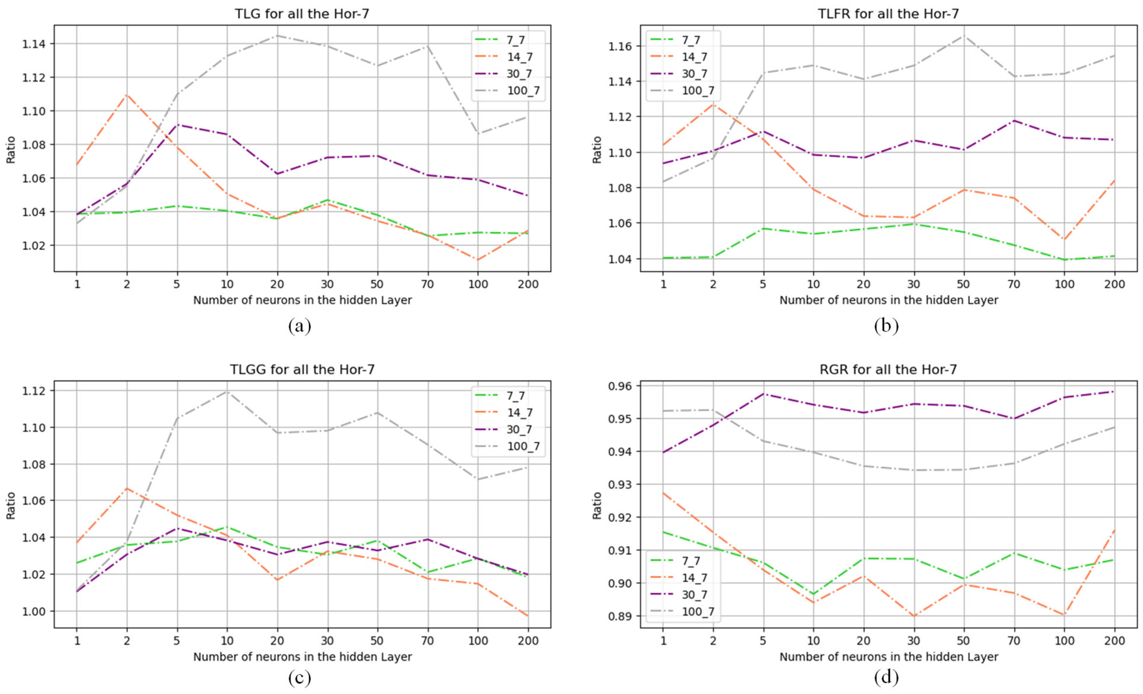
5.4. Results Discussion

The observations from Figure 6, Figure 7, Figure 8 and Figure 9 indicate that for Hor-1 and Hor-7 combinations, ePerf values decrease with the increase in the number of neurons in hidden layers. Nevertheless, the ePerfs values for Hor-1 combinations are lower compared to those for Hor-7. In the experiments, the ensemble consisting of four learner instances was evaluated against a single-instance setup. Even though the figure is not included, experimental results indicate that the decrease in ePerf values is steeper for the single-instance configuration than for the four-instance ensemble setup. This suggests that the ensemble configuration stabilizes the error decline. However, ePerf values are lower in the four-instance configuration than in the single-instance setup.
TLG exhibits a declining trend as the number of neurons in hidden layers (n) increases, for both Hor-1 and Hor-7 scenarios, except for the lag-hor (100-7) case, which only starts to decrease from n = 100. In Hor-1 scenarios, the higher the lag value, the higher the TLG.
Concerning TLFR, it shows a decreasing trend for Hor-1, where cases with smaller lag values are more susceptible to forgetting with the increase in the number of neurons in the hidden layer. Hor-7 combinations exhibit stability in terms of TLFR, though the lag 7 scenario displays a certain susceptibility to forgetting, with TLFR being approximately 1.
TLGG similarly demonstrates a declining trend for both Hor-1 and Hor-7 combinations, with TLGG decreasing as the number of neurons in the hidden layer increases. However, in Hor-1 scenarios, instances with higher lags exhibit greater TLGG compared to those with lower lags. Hor-7 combinations display a more gradual decline in TLGG, with the exception of the lag-hor (100-7) scenario, which exhibits a higher TLGG. Across both Hor-1 and Hor-7 combinations, scenarios with smaller lag values tend to approach TLGG ≈ 1, which is not yet a negative transfer.
Concerning RGR, every lag-hor combination within Hor-1 and Hor-7 demonstrates an inability to generalize in the target domain without further training, which proves the importance of transfer learning in ensuring generalization. However, it is observed that in Hor-1 scenarios, instances with higher lags exhibit reduced RGR compared to those with lower lags. Conversely, in Hor-7 scenarios, instances with lower lags display lower RGR than those with higher lags.
Thus, the experiments reveal that the ensemble learning setup, consisting of four instances, not only shields the model against the instability of ePerfs but also contributes to robustness by enhancing performance through improved TLG and TLGG and reduced TLFR, compared to the single-instance configuration. In most lag-hor configurations, TLG and TLGG are higher for a lower number of neurons in the hidden layer, n, and they decrease as n increases. Similarly, ePerf values also decrease with an increase in n. This implies that in the process of designing a neural network for transfer learning, it is essential to consider a trade-off or achieve a balance between the targeted TLG and the necessary ePerf value. We refer to this as a network dimensioning requirement for transfer learning, and we believe it could be an exciting area for future research to explore.

5.5. Assessment of the Use Case According to the Specification Book for a Comprehensive TSF TL Sensitivity Analysis

Table 4 provides a specification book for a comprehensive TSF TL Sensitivity Analysis. In Table 6, we assess the presented use case against this specification book.

6. Conclusions and Future Work

The field of transfer learning for time series forecasting is progressing, but it is still far from reaching maturity. Our study has filled a gap highlighted in recent survey papers, underscoring the importance of conducting empirical studies to develop practical guidelines for TL strategies and the selection or design of methods that can be employed by practitioners. The primary contribution of this paper has been the suggestion of a comprehensive framework for Transfer Learning Sensitivity Analysis for Time Series Forecasting. This has been achieved by identifying various parameters seen from various angles of transfer learning applied to time series, with the aim of uncovering factors and insights that influence the performance of transfer learning in time series forecasting. A further contribution has been the introduction of four TL performance metrics encompassed in the framework. After choosing the Ensemble TL technique as a use case, the results from the experiments of the sensitivity analysis of the Ensemble TL technique, have offered empirically informative insights into various parameters that impact the transfer learning gain, while raising the question of network dimensioning requirements, specifically, when designing a neural network for transfer learning. However, the implementation described in this paper has focused only on specific aspects of the parameters and dimensions mentioned within the framework of sensitivity analysis. By exploring future experiments from various angles and examining a broader array of dimensions, additional revelatory discoveries about the transfer learning process can be uncovered. For instance, in future experiments, considering various ML models configured with various shallow and/or deep architecture schemes while taking into account different clusters of the source and target domains, along with varying degrees of nonlinearity and homogeneity, can lead to interesting insights.

Author Contributions

Conceptualization, W.V.K. and K.K.; methodology, W.V.K., M.S., F.A.M. and K.K.; software, W.V.K., M.S. and K.K.; validation, W.V.K., T.B. and F.A.M.; writing—original draft preparation, W.V.K. and K.K.; writing—review and editing, M.S., T.B., F.A.M. and K.K.; visualization, W.V.K., M.S. and K.K.; supervision, F.A.M. and K.K.; formal analysis, W.V.K. and K.K.; project administration, W.V.K., M.S. and K.K. All authors have read and agreed to the published version of the manuscript.

Funding

This research received no external funding.

Data Availability Statement

Data are contained within the article.

Acknowledgments

The authors would like to express their gratitude to OeAD—Austria’s Agency for Education and Internationalization for the financial support provided through the OeAD Sonderstipendien, Universität Klagenfurt.

Conflicts of Interest

The authors declare no conflicts of interest.

References

  1. Torres, J.F.; Hadjout, D.; Sebaa, A.; Martínez-Álvarez, F.; Troncoso, A. Deep learning for time series forecasting: A survey. Big Data 2021, 9, 3–21. [Google Scholar] [CrossRef]
  2. Boyko, N. Data Interpretation Algorithm for Adaptive Methods of Modeling and Forecasting Time Series. WSEAS Trans. Math. 2023, 22, 359–372. [Google Scholar] [CrossRef]
  3. Zhuang, F.; Qi, Z.; Duan, K.; Xi, D.; Zhu, Y.; Zhu, H.; Xiong, H.; He, Q. A Comprehensive Survey on Transfer Learning. Proc. IEEE 2021, 109, 43–76. [Google Scholar] [CrossRef]
  4. Pan, S.J.; Yang, Q. A survey on transfer learning. IEEE Trans. Knowl. Data Eng. 2009, 22, 1345–1359. [Google Scholar] [CrossRef]
  5. Amaral, T.; Silva, L.M.; Alexandre, L.A.; Kandaswamy, C.; de Sá, J.M.; Santos, J.M. Transfer Learning Using Rotated Image Data to Improve Deep Neural Network Performance. In Proceedings of the International Conference Image Analysis and Recognition, Vilamoura, Portugal, 22–24 October 2014; Springer: Cham, Switzerland, 2014; pp. 290–300. [Google Scholar]
  6. Vu, N.T.; Imseng, D.; Povey, D.; Motlicek, P.; Schultz, T.; Bourlard, H. Multilingual deep neural network based acoustic modeling for rapid language adaptation. In Proceedings of the 2014 IEEE International Conference on Acoustics, Speech and Signal Processing (ICASSP), Florence, Italy, 4–9 May 2014; pp. 7639–7643. [Google Scholar]
  7. Fawaz, H.I.; Forestier, G.; Weber, J.; Idoumghar, L.; Muller, P.A. Transfer learning for time series classification. In Proceedings of the 2018 IEEE International Conference on Big Data (Big Data), Seattle, WA, USA, 10–13 December 2018; pp. 1367–1376. [Google Scholar]
  8. He, Q.Q.; Pang, P.C.I.; Si, Y.W. Transfer learning for financial time series forecasting. In PRICAI 2019: Trends in Artificial Intelligence: 16th Pacific Rim International Conference on Artificial Intelligence, Cuvu, Yanuca Island, Fiji, 26–30 August 2019; Springer: Cham, Switzerland, 2019; Volume 2, pp. 24–36. [Google Scholar]
  9. Mensink, T.; Uijlings, J.; Kuznetsova, A.; Gygli, M.; Ferrari, V. Factors of Influence for Transfer Learning Across Diverse Appearance Domains and Task Types. IEEE Trans. Pattern Anal. Mach. Intell. 2021, 44, 9298–9314. [Google Scholar] [CrossRef]
  10. Weber, M.; Auch, M.; Doblander, C.; Mandl, P.; Jacobsen, H.-A. Transfer Learning with Time Series Data: A Systematic Mapping Study. IEEE Access 2021, 9, 165409–165432. [Google Scholar] [CrossRef]
  11. Yan, P.; Abdulkadir, A.; Rosenthal, M.; Schatte, G.A.; Grewe, B.F.; Stadelmann, T. A comprehensive survey of deep transfer learning for anomaly detection in industrial time series: Methods, applications, and directions. arXiv 2023, arXiv:2307.05638. [Google Scholar] [CrossRef]
  12. Kumar, J.S.; Anuar, S.; Hassan, N.H. Transfer Learning based Performance Comparison of the Pre-Trained Deep Neural Networks. Int. J. Adv. Comput. Sci. Appl. 2022, 13. [Google Scholar] [CrossRef]
  13. Wang, B.; Mendez, J.; Cai, M.; Eaton, E. Transfer learning via minimizing the performance gap between domains. Adv. Neural Inf. Process. Syst. 2019, 32. [Google Scholar]
  14. Weiss, K.R.; Khoshgoftaar, T.M. Analysis of transfer learning performance measures. In Proceedings of the 2017 IEEE International Conference on Information Reuse and Integration (IRI), San Diego, CA, USA, 4–6 August 2017; pp. 338–345. [Google Scholar]
  15. Weiss, K.; Khoshgoftaar, T.M.; Wang, D.D. A survey of transfer learning. J. Big Data 2016, 3, 1345–1459. [Google Scholar] [CrossRef]
  16. Willard, J.D.; Read, J.S.; Appling, A.P.; Oliver, S.K.; Jia, X.; Kumar, V. Predicting Water Temperature Dynamics of Unmonitored Lakes with Meta-Transfer Learning. Water Resour. Res. 2021, 57, e2021WR029579. [Google Scholar] [CrossRef]
  17. Gaddipati, S.K.; Nair, D.; Plöger, P.G. Comparative evaluation of pretrained transfer learning models on automatic short answer grading. arXiv 2020, arXiv:2009.01303. [Google Scholar]
  18. Bao, Y.; Li, Y.; Huang, S.-L.; Zhang, L.; Zheng, L.; Zamir, A.; Guibas, L. An Information-Theoretic Approach to Transferability in Task Transfer Learning. In Proceedings of the 2019 IEEE International Conference on Image Processing (ICIP), Taipei, Taiwan, 22–25 September 2019; pp. 2309–2313. [Google Scholar]
  19. Ben-David, S.; Schuller, R. Exploiting Task Relatedness for Multiple Task Learning; Lecture Notes in Computer Science; Springer: Berlin/Heidelberg, Germany, 2003; pp. 567–580. [Google Scholar]
  20. Liao, T.W. Clustering of time series data—A survey. Pattern Recognit. 2005, 38, 1857–1874. [Google Scholar] [CrossRef]
  21. Wang, J.; Chen, Y.; Feng, W.; Yu, H.; Huang, M.; Yang, Q. Transfer Learning with Dynamic Distribution Adaptation. ACM Trans. Intell. Syst. Technol. 2020, 11, 1–25. [Google Scholar] [CrossRef]
  22. Zhang, W.; Deng, L.; Zhang, L.; Wu, D. A Survey on Negative Transfer. IEEE/CAA J. Autom. Sin. 2022, 10, 305–329. [Google Scholar] [CrossRef]
  23. Kemker, R.; McClure, M.; Abitino, A.; Hayes, T.; Kanan, C. Measuring Catastrophic Forgetting in Neural Networks. In Proceedings of the Thirty-Second AAAI Conference on Artificial Intelligence, New Orleans, LA, USA, 2–7 February 2018; Volume 32. [Google Scholar] [CrossRef]
  24. Abraham, W.C.; Robins, A. Memory retention—The synaptic stability versus plasticity dilemma. Trends Neurosci. 2005, 28, 73–78. [Google Scholar] [CrossRef]
  25. Chen, X.; Wang, S.; Fu, B.; Long, M.; Wang, J. Catastrophic forgetting meets negative transfer: Batch spectral shrinkage for safe transfer learning. Adv. Neural Inf. Process. Syst. 2019, 32. [Google Scholar]
  26. Mahmoud, R.A.; Hajj, H. Multi-objective Learning to Overcome Catastrophic Forgetting in Time-series Applications. ACM Trans. Knowl. Discov. Data 2022, 16, 1–20. [Google Scholar] [CrossRef]
  27. Ge, L.; Gao, J.; Ngo, H.; Li, K.; Zhang, A. On Handling Negative Transfer and Imbalanced Distributions in Multiple Source Transfer Learning. Stat. Anal. Data Min. ASA Data Sci. J. 2014, 7, 254–271. [Google Scholar] [CrossRef]
  28. Niu, S.; Liu, Y.; Wang, J.; Song, H. A decade survey of transfer learning (2010–2020). IEEE Trans. Artif. Intell. 2020, 1, 151–166. [Google Scholar] [CrossRef]
  29. Peirelinck, T.; Kazmi, H.; Mbuwir, B.V.; Hermans, C.; Spiessens, F.; Suykens, J.; Deconinck, G. Transfer learning in demand response: A review of algorithms for data-efficient modelling and control. Energy AI 2021, 7, 100126. [Google Scholar] [CrossRef]
  30. Zhang, R.; Tao, H.; Wu, L.; Guan, Y. Transfer Learning with Neural Networks for Bearing Fault Diagnosis in Changing Working Conditions. IEEE Access 2017, 5, 14347–14357. [Google Scholar] [CrossRef]
  31. Kearney, D.; McLoone, S.; Ward, T.E. Investigating the Application of Transfer Learning to Neural Time Series Classification. In Proceedings of the 2019 30th Irish Signals and Systems Conference (ISSC), Maynooth, Ireland, 17–18 June 2019; pp. 1–5. [Google Scholar]
  32. Fan, C.; Sun, Y.; Xiao, F.; Ma, J.; Lee, D.; Wang, J.; Tseng, Y.C. Statistical investigations of transfer learning-based methodology for short-term building energy predictions. Appl. Energy 2020, 262, 114499. [Google Scholar] [CrossRef]
  33. Taleb, C.; Likforman-Sulem, L.; Mokbel, C.; Khachab, M. Detection of Parkinson’s disease from handwriting using deep learning: A comparative study. Evol. Intell. 2020, 16, 1813–1824. [Google Scholar] [CrossRef]
  34. Marczewski, A.; Veloso, A.; Ziviani, N. Learning transferable features for speech emotion recognition. In Proceedings of the Thematic Workshops of ACM Multimedia 2017, Mountain View, CA, USA, 23–27 October 2017; pp. 529–536. [Google Scholar]
  35. Mun, S.; Shon, S.; Kim, W.; Han, D.K.; Ko, H. Deep Neural Network based learning and transferring mid-level audio features for acoustic scene classification. In Proceedings of the 2017 IEEE International Conference on Acoustics, Speech and Signal Processing (ICASSP), New Orleans, LA, USA, 5–9 March 2017; pp. 796–800. [Google Scholar]
  36. Matsui, S.; Inoue, N.; Akagi, Y.; Nagino, G.; Shinoda, K. User adaptation of convolutional neural network for human activity recognition. In Proceedings of the 2017 25th European Signal Processing Conference (EUSIPCO), Kos Island, Greece, 28 August–2 September 2017; pp. 753–757. [Google Scholar]
  37. Goodfellow, I.J.; Pouget-Abadie, J.; Mirza, M.; Xu, B.; Warde-Farley, D.; Ozair, S.; Courville, A.; Bengio, Y. Generative adversarial networks. Proc. Adv. Neural Inf. Process. Syst. 2014, 2672–2680. [Google Scholar] [CrossRef]
  38. Ganin, Y.; Ustinova, E.; Ajakan, H.; Germain, P.; Larochelle, H.; Laviolette, F.; Marchand, M.; Lempitsky, V. Domain-Adversarial Training of Neural Networks. J. Mach. Learn. Res. 2015, 17, 2030–2096. [Google Scholar] [CrossRef]
  39. Tang, Y.; Qu, A.; Chow, A.H.; Lam, W.H.; Wong, S.C.; Ma, W. Domain adversarial spatial-temporal network: A transferable framework for short-term traffic forecasting across cities. In Proceedings of the 31st ACM International Conference on Information & Knowledge Management, Atlanta, GA, USA, 17–21 October 2022; pp. 1905–1915. [Google Scholar]
  40. Chen, L.; Peng, C.; Yang, C.; Peng, H.; Hao, K. Domain adversarial-based multi-source deep transfer network for cross-production-line time series forecasting. Appl. Intell. 2023, 53, 22803–22817. [Google Scholar] [CrossRef]
  41. Hernandez, J.; Morris, R.R.; Picard, R.W. Call Center Stress Recognition with Person-Specific Models. In Proceedings of the International Conference on Affective Computing and Intelligent Interaction, Memphis, TN, USA, 9–12 October 2011; pp. 125–134. [Google Scholar]
  42. Li, X.; Zhang, W.; Ding, Q.; Sun, J.-Q. Multi-Layer domain adaptation method for rolling bearing fault diagnosis. Signal Process. 2018, 157, 180–197. [Google Scholar] [CrossRef]
  43. Zhu, J.; Chen, N.; Shen, C. A New Deep Transfer Learning Method for Bearing Fault Diagnosis Under Different Working Conditions. IEEE Sens. J. 2019, 20, 8394–8402. [Google Scholar] [CrossRef]
  44. Wang, X.; Zhu, C.; Jiang, J. A deep learning and ensemble learning based architecture for metro passenger flow forecast. IET Intell. Transp. Syst. 2023, 17, 487–502. [Google Scholar] [CrossRef]
  45. Dai, W.; Yang, Q.; Xue, G.-R.; Yu, Y. Boosting for transfer learning. In Proceedings of the ICML ‘07 & ILP ‘07: The 24th Annual International Conference on Machine Learning held in conjunction with the 2007 International Conference on Inductive Logic Programming, Corvallis, OR, USA, 19–21 June 2007; pp. 193–200. [Google Scholar]
  46. Deo, R.V.; Chandra, R.; Sharma, A. Stacked transfer learning for tropical cyclone intensity prediction. arXiv 2017, arXiv:1708.06539. [Google Scholar]
  47. Daumé, H., III. Frustratingly easy domain adaptation. In Proceedings of the 45th Annual Meeting of the Association for Computational Linguistics, Prague, Czech Republic, 23–30 June 2007; pp. 256–263. [Google Scholar]
  48. Fernando, B.; Habrard, A.; Sebban, M.; Tuytelaars, T. Unsupervised Visual Domain Adaptation Using Subspace Alignment. In Proceedings of the 2013 IEEE International Conference on Computer Vision (ICCV), Sydney, Australia, 1–8 December 2013; pp. 2960–2967. [Google Scholar]
  49. Blitzer, J.; McDonald, R.; Pereira, F. Domain adaptation with structural correspondence learning. In Proceedings of the 2006 Conference on Empirical Methods in Natural Language Processing (EMNLP), Sydney, Australia, 22–23 July 2006; pp. 120–128. [Google Scholar]
  50. Deng, J.; Zhang, Z.; Marchi, E.; Schuller, B. Sparse Autoencoder-Based Feature Transfer Learning for Speech Emotion Recognition. In Proceedings of the 2013 Humaine Association Conference on Affective Computing and Intelligent Interaction, Geneva, Switzerland, 2–5 September 2013; pp. 511–516. [Google Scholar]
  51. Banerjee, D.; Islam, K.; Mei, G.; Xiao, L.; Zhang, G.; Xu, R.; Ji, S.; Li, J. A Deep Transfer Learning Approach for Improved Post-Traumatic Stress Disorder Diagnosis. In Proceedings of the 2017 IEEE International Conference on Data Mining (ICDM), New orleans, LA, USA, 18–21 November 2017; pp. 11–20. [Google Scholar]
  52. Wang, T.; Huan, J.; Zhu, M. Instance-based deep transfer learning. In Proceedings of the 2019 IEEE Winter Conference on Applications of Computer Vision (WACV), Waikoloa Village, HI, USA, 7–11 January 2019; pp. 367–375. [Google Scholar]
  53. Kim, J.; Lee, J. Instance-based transfer learning method via modified domain-adversarial neural network with influence function: Applications to design metamodeling and fault diagnosis. Appl. Soft Comput. 2022, 123, 108934. [Google Scholar] [CrossRef]
  54. Yin, Z.; Wang, Y.; Liu, L.; Zhang, W.; Zhang, J. Cross-Subject EEG Feature Selection for Emotion Recognition Using Transfer Recursive Feature Elimination. Front. Neurorobot. 2017, 11, 19. [Google Scholar] [CrossRef]
  55. Villar, J.R.; de la Cal, E.; Fañez, M.; González, V.M.; Sedano, J. Usercentered fall detection using supervised, on-line learning and transfer learning. Prog. Artif. Intell. 2019, 8, 453–474. [Google Scholar] [CrossRef]
  56. Chen, T.; Guestrin, C. XGBoost: A scalable tree boosting system. In Proceedings of the 22nd ACM SIGKDD International Conference on Knowledge Discovery and Data Mining, San Francisco, CA, USA, 13–17 August 2016; pp. 785–794. [Google Scholar]
  57. Shen, S.; Sadoughi, M.; Li, M.; Wang, Z.; Hu, C. Deep convolutional neural networks with ensemble learning and transfer learning for capacity estimation of lithium-ion batteries. Appl. Energy 2020, 260, 114296. [Google Scholar] [CrossRef]
  58. Di, Z.; Shao, H.; Xiang, J. Ensemble deep transfer learning driven by multisensor signals for the fault diagnosis of bevel-gear cross-operation conditions. Sci. China Technol. Sci. 2021, 64, 481–492. [Google Scholar] [CrossRef]
  59. Ingalls, B. Sensitivity analysis: From model parameters to system behaviour. Essays Biochem. 2008, 45, 177–194. [Google Scholar] [CrossRef]
  60. Tu, W.; Sun, S. A subject transfer framework for EEG classification. Neurocomputing 2012, 82, 109–116. [Google Scholar] [CrossRef]
  61. Natarajan, A.; Angarita, G.; Gaiser, E.; Malison, R.; Ganesan, D.; Marlin, B.M. Domain adaptation methods for improving lab-to-field generalization of cocaine detection using wearable ECG. In Proceedings of the UbiComp ‘16: The 2016 ACM International Joint Conference on Pervasive and Ubiquitous Computing, Heidelberg, Germany, 12–16 September 2016; pp. 875–885. [Google Scholar]
  62. Day, O.; Khoshgoftaar, T.M. A survey on heterogeneous transfer learning. J. Big Data 2017, 4, 29. [Google Scholar] [CrossRef]
  63. Ritter, H.; Botev, A.; Barber, D. Online structured laplace approximations for overcoming catastrophic forgetting. Adv. Neural Inf. Process. Syst. 2018, 31. [Google Scholar]
  64. Kirkpatrick, J.; Pascanu, R.; Rabinowitz, N.; Veness, J.; Desjardins, G.; Rusu, A.A.; Milan, K.; Quan, J.; Ramalho, T.; Grabska-Barwinska, A.; et al. Overcoming catastrophic forgetting in neural networks. Proc. Natl. Acad. Sci. USA 2017, 114, 3521–3526. [Google Scholar] [CrossRef]
  65. Peng, J.; Hao, J.; Li, Z.; Guo, E.; Wan, X.; Min, D.; Zhu, Q.; Li, H. Overcoming Catastrophic Forgetting by Soft Parameter Pruning. arXiv 2018, arXiv:1812.01640. [Google Scholar]
  66. Solak, A.; Ceylan, R. A sensitivity analysis for polyp segmentation with U-Net. Multimed. Tools Appl. 2023, 82, 34199–34227. [Google Scholar] [CrossRef]
  67. . Long, M.; Wang, J.; Ding, G.; Pan, S.J.; Yu, P.S. Adaptation Regularization: A General Framework for Transfer Learning. IEEE Trans. Knowl. Data Eng. 2013, 26, 1076–1089. [Google Scholar] [CrossRef]
  68. . Abbas, A.; Abdelsamea, M.M.; Gaber, M.M. DeTrac: Transfer Learning of Class Decomposed Medical Images in Convolutional Neural Networks. IEEE Access 2020, 8, 74901–74913. [Google Scholar] [CrossRef]
  69. . Guo, H.; Zhuang, X.; Chen, P.; Alajlan, N.; Rabczuk, T. Analysis of three-dimensional potential problems in non-homogeneous media with physics-informed deep collocation method using material transfer learning and sensitivity analysis. Eng. Comput. 2022, 38, 5423–5444. [Google Scholar] [CrossRef]
  70. Tsay, R.S. Nonlinearity tests for time series. Biometrika 1986, 73, 461–466. [Google Scholar] [CrossRef]
  71. Whitcher, B.; Byers, S.D.; Guttorp, P.; Percival, D.B. Testing for homogeneity of variance in time series: Long memory, wavelets, and the Nile River. Water Resour. Res. 2002, 38, 12-1–12-16. [Google Scholar] [CrossRef]
  72. Golestani, A.; Gras, R. Can we predict the unpredictable? Sci. Rep. 2014, 4, 6834. [Google Scholar] [CrossRef] [PubMed]
  73. Soekhoe, D.; Van Der Putten, P.; Plaat, A. On the impact of data set size in transfer learning using deep neural networks. In Proceedings of the Advances in Intelligent Data Analysis XV: 15th International Symposium, IDA 2016, Stockholm, Sweden, 13–15 October 2016; Proceedings 15. Springer International Publishing: Cham, Switzerland, 2016; pp. 50–60. [Google Scholar]
  74. Liu, A.; Liu, X.; Yu, H.; Zhang, C.; Liu, Q.; Tao, D. Training Robust Deep Neural Networks via Adversarial Noise Propagation. IEEE Trans. Image Process. 2021, 30, 5769–5781. [Google Scholar] [CrossRef] [PubMed]
  75. Cisse, M.; Bojanowski, P.; Grave, E.; Dauphin, Y.; Usunier, N. Parseval networks: Improving robustness to adversarial examples. In Proceedings of the International Conference on Machine Learning, Sydney, Australia, 6–11 August 2017. [Google Scholar]
  76. Chin, T.W.; Zhang, C.; Marculescu, D. Renofeation: A simple transfer learning method for improved adversarial robustness. In Proceedings of the IEEE/CVF Conference on Computer Vision and Pattern Recognition, Nashville, TN, USA, 20–25 June 2021; pp. 3243–3252. [Google Scholar]
  77. Deng, Z.; Zhang, L.; Vodrahalli, K.; Kawaguchi, K.; Zou, J.Y. Adversarial training helps transfer learning via better representations. Adv. Neural Inf. Process. Syst. 2021, 34, 25179–25191. [Google Scholar]
  78. Littlestone, N.; Warmuth, M. The Weighted Majority Algorithm. Comput. Eng. Inf. Sci. 1994, 108, 212–261. [Google Scholar] [CrossRef]
  79. Breiman, L. Bagging predictors. Mach. Learn. 1996, 24, 123–140. [Google Scholar] [CrossRef]
  80. Duin, R. The combining classifier: To train or not to train? In Proceedings of the 16th International Conference on Pattern Recognition, Quebec City, QC, Canada, 11–15 August 2002; pp. 765–770. [Google Scholar]
Figure 1. Illustration of the five performance assessment scenarios.
Symmetry 16 00241 g001
Figure 2. TL approaches applicable to time series (source [10]).
Symmetry 16 00241 g002
Figure 3. Domain adversarial neural network [38].
Symmetry 16 00241 g003
Figure 4. Relevant TSF-related TL sensitivity analysis contextual dimensions.
Symmetry 16 00241 g004
Figure 5. The three main ensemble learning techniques.
Symmetry 16 00241 g005
Figure 6. (ad) ePerf values for the Hor-1 combinations ((7,1), (14,1), (30,1), (100,1)).
Symmetry 16 00241 g006
Figure 7. (ad) ePerf values for the Hor-7 combinations ((7,7), (14,7), (30,7), (100,7)).
Symmetry 16 00241 g007
Figure 8. (ad) TL Metrics for the Hor-1 combinations ((7,1), (14,1), (30,1), (100,1)).
Symmetry 16 00241 g008
Figure 9. (ad) TL Metrics for the Hor-7 combinations ((7,7), (14,7), (30,7), (100,7)).
Symmetry 16 00241 g009
Table 1. Definition of the performance assessment scenarios.
Performance
Analysis Scenario
ModelTrainingTestPerformance
Metric
Scenario 1Model 1Training data 1Test data 1ePerf1
Scenario 2Model 2/ATraining data 2Test data 2ePerf2
Scenario 3Model 1Training data 1Test data 2ePerf3
Scenario 4Model 2/ATraining data 2Test data 1ePerf4
Scenario 5Model 2/BTraining data 2Test data 2ePerf5
Table 2. Explanation of the different types of Transfer Learning.
Type of Transfer LearningWhat Is Transferred
Model-basedParameters of a pre-trained model
Feature-basedFeatures learned by a pre-trained model
Instance-basedTraining examples from the source domain
Table 4. Specification book for a comprehensive TSF TL Sensitivity Analysis.
RequirementExplanation of the Requirement
Source modelA pre-trained model is required to serve as the source model for the transfer learning process. The source model should be trained on a related task or domain to the target task or domain.
DataSufficient data are required for both the source and target tasks. The source task should have a large amount of labeled data, while the target task may have limited labeled data.
SimilarityThere should be some similarity between the source and target tasks or domains. The more similar they are, the more effective the transfer learning process will be.
TL design (layer selection)A TL design needs to be determined beforehand. For neural networks, the selection of which layers to update and which to fix is an important consideration in transfer learning. The choice of layers will depend on the specific task and data.
Hyperparameter tuningHyperparameters such as learning rate, batch size, and number of epochs need to be tuned to optimize the performance of the transfer learning model.
Evaluation metricsAppropriate evaluation metrics need to be selected to measure the performance of the transfer learning model. The choice of metrics will depend on the specific task and data.
Baseline modelEstablish baseline models, either trained from scratch or using other transfer learning techniques, to compare and contrast the performance
Computational requirementsDefine the acceptable computational time and resources for the transfer learning process. The efficiency of transfer learning is often a consideration, especially when deployment resources are constrained.
Model robustnessDefine requirements for the model’s stability and robustness against adversarial attacks, noise, or other perturbations, especially in critical applications
Negative transfer avoidancePut mechanisms in place to detect or avoid negative transfer, where transfer learning leads to degraded performance.
ReproducibilityThe evaluation process should be reproducible. This might involve requirements about documentation, random seed settings, or the clarity of the process and methods used.
Table 5. Selected Sensitivity Analysis parameters.
ParametersConfiguration
Ensemble technique usedBagging
Number of ensemble instances4
Type of neural networkMLP
Number of hidden layers1 (shallow network)
Number of neurons1, 2, 5, 10, 20, 30, 50, 70, 100, and 200
Lag size and horizon size(7, 1), (14, 1), (30, 1), (100, 1)
(7, 7), (14, 7), (30, 7), and (100, 7)
Evaluation metricsTLG, TLFR, RGR, and TLGG
(defined in Section 2.4)
(Dis)similarity metrics to assess the distance between source and target domainsPearson, DTW
Table 6. Assessment of the use case against the specification book for a comprehensive TSF TL Sensitivity Analysis.
RequirementAssessment of the Use Case
Source modelA source model was pre-trained for later use in the target domain.
DataSufficient data were available to train the source model.
SimilarityThe calculated Pearson distance between the source and target datasets (PD = 0.9105) shows a degree of similarity between the source and target domains.
TL design (layer selection)In this case, a shallow MLP was used.
Hyperparameter tuningHyperparameters (learning rate, batch size, and number of epochs) were set to optimize the performance of the transfer learning model.
Evaluation metricsThe proposed TL metrics were used.
Baseline modelNo baseline model was explicitly chosen; however, various performance analysis scenarios were set up, with selected scenarios being considered as baselines in the analysis (see Table 1).
Computational requirementsComputational requirements were not explicitly monitored; the focus was more on the sensitivity analysis of other dimensions.
Model robustnessRequirements for the model’s robustness against adversarial attacks, noise, or other perturbations were not considered in the use case. These will be considered in further study.
Negative transfer avoidanceThe aim set for the study was to gain insight into the possible vulnerability of the network to negative transfer and catastrophic forgetting, not to eliminate them.
ReproducibilityThe source code is available on request for reproducibility.
Disclaimer/Publisher’s Note: The statements, opinions and data contained in all publications are solely those of the individual author(s) and contributor(s) and not of MDPI and/or the editor(s). MDPI and/or the editor(s) disclaim responsibility for any injury to people or property resulting from any ideas, methods, instructions or products referred to in the content.

