
Mapping GENERIC Hydrodynamics into Carter’s Multifluid Theory


Department of Mathematics, Vanderbilt University, Nashville, TN 37240, USA
Symmetry 2024, 16(1), 78; https://doi.org/10.3390/sym16010078
Submission received: 9 December 2023
/
Revised: 3 January 2024
/
Accepted: 4 January 2024
/
Published: 6 January 2024
(This article belongs to the Special Issue Relativistic Hydrodynamics and Symmetry: Theory, Methods and Applications)
Abstract
:We show that the GENERIC model for relativistic heat conduction is a multifluid of Carter; this allows one to compute the multifluid constitutive relations directly from the GENERIC formalism. As a quick application, we prove that in the limit of infinite heat conductivity, GENERIC heat conduction reduces to the relativistic two-fluid model for superfluidity. This surprising “crossover” is a consequence of relativistic causality: if diffusion happens too fast, all the diffusing charge cumulates on the surface of the light cone, and it eventually travels at the speed of light like a wave. Our analysis is non-perturbative and carried out in a fully non-linear regime.
1. Introduction
Most of the relativistic hydrodynamic theories currently in use rely on some form of near-equilibrium expansion. For example, the original Israel–Stewart theory arises from a perturbative expansion for small viscous fluxes [1,2,3,4], while BRSSS [5] and BDNK [6] arise from an expansion for small gradients. DNMR arises from a subtle combination of the two expansions above [7]. While these approaches have the advantage of being systematic and rigorous, the resulting fluid models usually have a limited formal regime of applicability, and they may not capture all those intrinsically non-linear phenomena that real-world substances are known to exhibit. This kind of problem is well known to material engineers since, in our everyday life, we deal with many non-Newtonian fluids that easily escape a Navier–Stokes description [8]. Indeed, most foods and toiletry products explore dynamical regimes where the shear stress component, say, , grows like a fractional power of the symmetrized velocity gradient [9]. For example, the shear stress of ketchup at 30.5 C exhibits the following non-Newtonian behavior:
Clearly, features of this kind are hardly captured by conventional gradient expansions.
Since the rheological properties of hadronic and quark matter are poorly known, we cannot exclude that non-perturbative corrections to the constitutive relations might be important for neutron star mergers and heavy-ion phenomenology. If that were the case, relativistic viscous hydrodynamics as we know it would be non-reliable for most practical applications, and we would need a full-fledged theory of relativistic rheology. At present, a fully general and rigorous theory of this kind exists only in the linear regime [10], and we are still unable to describe non-perturbative phenomena systematically. Still, some isolated “non-linear rheological models” have been formulated, such as Anisotropic Hydrodynamics [11,12], which models shear viscosity non-perturbatively, and Hydro+ [13,14], which models bulk viscosity non-perturbatively. The question of how to model non-perturbative corrections to heat conduction is still an open problem, and it is the subject of investigation in the present article.
First, a bit of history. The interplay between heat conduction and relativity has had a long (and controversial) development. The source of all problems is a technicality: if , then “flow of energy” = “density of momentum” (i.e., [15]). As a consequence, heat carries inertia, and it is practically impossible to disentangle exchanges of heat from macroscopic accelerations [16]; this is a natural consequence of the relativistic duality between energy and momentum, but failure to recognize it has generated some confusion over the definition of thermal equilibrium in relativity [17]. This subtlety is also at the origin of the (unphysical) heat-driven accelerations predicted by the Eckart theory [18], and of the ambiguity between the Eckart and the Landau–Lifshitz hydrodynamic frames [4].
The modern theory of relativistic heat conduction was pioneered by Carter [19,20]. He started from the observation that if the heat carries inertia, then the four-momentum of the fluid must be “redistributed” between the entropy current and the particle current . By symmetry, the most general way of distributing the four-momentum is
where P, , , and are functions of and ; this gives rise to a “two-fluid model” for heat conduction, where dissipation is represented as friction between the two currents and . Not surprisingly, one can show that when the currents are almost collinear, Carter’s theory reduces to the Israel–Stewart theory [21,22,23]. However, one can, in principle, extend the constitutive relations of P, , , to states where the angle between and is large, allowing one to model heat conduction in non-perturbative regimes [24].
Unfortunately, at present, the applicability of Carter’s theory to non-perturbative regimes remains merely hypothetical. In fact, there is no concrete proposal for the constitutive relations of P, , , and beyond the Israel–Stewart limit. In this brief article, we present a novel and rigorous result which might be helpful in this direction. In fact, here we prove that there is an exact change in variables that maps the GENERIC theory (GENERIC is an acronym for “General Equation for the NonEquilibrium Reversible-Irreversible Coupling” [25]. It is grounded on the assumption that the equations of motion of any non-equilibrium thermodynamic system, with degrees of freedom , can be expressed in the form , where is a reversible Hamiltonian part and is an irreversible entropy-driven Lyapunov part) for non-linear heat conduction developed by Öttinger [26] into Carter’s multifluid theory. This implies that it is possible to derive the constitutive relations of Carter’s theory directly from the GENERIC formalism [25,27]. Since the latter was designed with the very purpose of modeling non-perturbative phenomena in complex fluids [27], this might be our only way of deriving Carter’s theory for heat conduction directly from microphysics.
Throughout this paper, we adopt the metric signature , and work in natural units: .
2. Relativistic Dissipative Hydrodynamics in a Nutshell
Historically, there have been two different ways of modeling dissipation in a hydrodynamic setting. One is the so-called “gradient expansion”, where the degrees of freedom of the theory are the ordinary fluid fields , representing, respectively, temperature, chemical potential, and flow velocity (each field corresponds to a conservation law, respectively energy, particles, and momentum [28,29]), and the stress–energy tensor is expanded in powers of gradients of such variables, e.g., . This approach goes back to Navier and Stokes [30] and Burnett [31], and it is often invoked as the main rationale for viscous hydrodynamics [5,32,33]. The second is known as “Extended Irreversible Thermodynamics” [34] (EIT), and it consists of adding new non-equilibrium variables besides the usual fluid ones, i.e., . This expands the state space of the fluid, enabling dissipation when the new variables differ from their local equilibrium values. These extended fluid variables fully characterize all the properties of the fluid at a given event . Thus, no gradient corrections are needed, i.e., . This approach was pioneered by Maxwell [35], Cattaneo [36], and Muller [37], and it finds many applications in the theory of viscoelasticity [9,38,39,40,41].
To better visualize the difference between the two approaches, consider the problem of deriving hydrodynamics from kinetic theory. In this setting, the goal is to express the one-particle distribution function in terms of a set of fluid fields , i.e., . Then, the relativistic Boltzmann equation [15,42]
written in terms of , can be used to derive some approximate equations of motion for the fluid fields.
In the ideal fluid limit, the distribution is locally Fermi–Dirac for Fermions, or Bose–Einstein for Bosons, so that
This clearly shows that, for ideal fluids, the natural field degrees of freedom are . Indeed, by substituting (4) into (3), one can easily derive the equations of motion for the ideal fluid [43].
In the dissipative case, one needs to model the non-equilibrium deviations from (4). In the gradient expansion approach, one still assumes that , but now becomes a functional of , i.e.,
where depends on the value of in a (possibly large) neighborhood of the event under consideration. Now, if T, , and are analytic across , their behavior in the neighborhood is uniquely determined by the values of all their infinite derivatives at [44] so that
Expanding in powers of derivatives leads to viscous theories, such as relativistic Navier–Stokes [30,45], BDNK [6,46,47], BRSSS [5], and IRED [48]. Adding up all the terms of the series of usually leads to a divergence. However, with the aid of Borel resummation, one can reconstruct, in some cases, the exact value of [49,50,51,52].
The approach of Extended Irreversible Thermodynamics is different. Here, one parameterizes the quantity in Equation (5) in terms of some structural fields , which determine its analytical form. For example, one may express as a series , where form a basis of [15]. This results in a theory with hydrodynamic fields , and distribution function
No information about the local gradients enters the formula for (and thus that of ). Instead, the gradients appear when we substitute (7) into (3). This produces some equations of motion for , where the local gradients appear as sources. If we truncate the sequence of (invoking some power counting scheme) and keep only the most relevant variables, we recover transient hydrodynamic theories, such as Israel–Stewart hydrodynamics [1], DNMR [53] (in part [7]), the divergence-type theory [54], and maximum entropy hydrodynamics [55]. Carter’s theory and the GENERIC adopt the EIT approach, too. Therefore, we will stick here to interpretation (7).
We remark that one should not view (5) and (7) as contradictory to each other. Rather, they are different techniques for approximating the same complicated system. As such, they focus on different aspects of the problem. The mathematical relationship between the two viewpoints has been studied systematically in several works [56,57,58,59].
3. Outline of Carter’s Multifluid Theory
In this section, we briefly review Carter’s multifluid theory. The reader can see [19,60,61,62,63,64,65] for an overview of the foundations of the formalism. For the purposes of this paper, it will be enough to adopt the generating function approach developed in [24]. Also, we will work in the “pressure & momenta” representation [23,66].
3.1. Multifluid Constitutive Relations
Our fundamental degrees of freedom are two (unconstrained) covectors, and , which are called momenta of the fluid. The number of algebraic degrees of freedom is, therefore, , following the Israel–Stewart theory for heat conduction (Carter’s theory does not pick a specific hydrodynamic frame, i.e., it is not explicit on the definitions of T, , and out of equilibrium. However, the “natural” frames take the form , , and [20,62,64]). We anticipate here that coincides with the homonymous structural variable introduced by Öttinger [26]. The multifluid equation of state of the system is an expression of the form
where P is the kinematic pressure of the multifluid transversal to the heat flux, and is the inverse metric tensor. The constitutive relations for the entropy current , the conserved particle current , and the (symmetric) stress–energy tensor are computed from the equation of state through the following differential:
Lorentz covariance implies that P can depend only on the scalars , , and (recall that, within Extended Irreversible Thermodynamics, gradients do not enter the constitutive relations; see Section 2). Therefore, we can express the differential of P in the following form [66]:
where C, A, and B are some non-equilibrium thermodynamic scalars. Substituting (10) into (9), we obtain
Note that the stress–energy tensor above has the form (2), and it is, therefore, symmetric, even if not manifestly so. The inverse of the matrix in the first equation of (11) is called the entrainment matrix, and it enters the quadratic form in Equation (2). Both the entrainment matrix and its inverse are positive definite by stability [23]. This results in three notable inequalities: , , and .
3.2. Multifluid Field Equations
The fields of the hydrodynamic theory are , which constitute eight algebraic degrees of freedom. Hence, we need eight independent equations of motion. Out of these, 5 are the conservation laws, , and . Invoking (10) and (11), the energy–momentum conservation can be equivalently rewritten in the form [62]
To complete the system, we need three additional equations of motion. The multifluid theory does not provide a unique choice for such an equation. Instead, it provides us with some reasonable options inspired by geometry and thermodynamics [19,20,24,65]. A rather convenient option is
which plays the role of an Israel–Stewart-type relaxation equation for the heat flux [24], where is a transport coefficient. Indeed, if we contract (12) with and use Equation (13), we find that the fluid produces entropy:
The non-negativity of the entropy production follows from the observation that the term in the round brackets on the right-hand side is the spacelike projector orthogonal to , and , so that
4. Recovering the GENERIC Theory
Let us now show that the multifluid model described above is mathematically equivalent to the GENERIC theory for heat conduction constructed by Öttinger [26], just expressed using different notations.
4.1. Decomposition of Tensors
The GENERIC theory adopts the Eckart frame, meaning that it defines a preferred four-velocity , aligned with the particle current: . The temperature and chemical potential are defined through the equations and . The vectors and are treated as primary vectors, meaning that all other tensors are geometrically decomposed as linear combinations of tensor products of . For example, and are expressed as
Since the inverse entrainment matrix is positive definite by stability, we have that and . If we substitute (16) into the multifluid formula for the stress–energy tensor as given in (11), we obtain
In accordance with the Eckart frame definition, we have that n and are indeed the particle and energy density as measured in the reference frame defined by , namely and .
4.2. First Law of Thermodynamics
In the GENERIC representation, the differential (9) at fixed metric components becomes
We can use the Leibnitz rule to rewrite this differential as follows:
The second equation of (16) can be rewritten in the form so that the last term in (20) vanishes. Furthermore, if we contract the second equation of (16) with , we obtain , which is in agreement with Equation (50) of [26]. This allows us to derive the following differential:
Our Equations (16), (18), and (21) are indeed consistent with Equations (39), (45), (54), (55), and (65) of [26] (note that Öttinger [26] splits the energy into rest mass part plus internal contributions, while we are combining them together; thus, the notation “” of [26] becomes just in our notation); this shows that the constitutive relations of the GENERIC theory can be recovered from the multifluid formalism, by simply expressing all equations in the Eckart frame.
4.3. Recovering the GENERIC Field Equations
To complete our analysis, we only need to verify that Equations (13) and (14) are indeed the dissipative equations of motion of the GENERIC theory. To this end, let us set , where is the heat relaxation time. Then, (13) and (14) become
which indeed coincide with Equations (73) and (75) of [26]. This completes the correspondence between the GENERIC and the multifluid theory. Note that no approximation was made, meaning that the “dictionary” is exact in the fully non-linear regime. For completeness, we summarize the GENERIC equations in Appendix A.
5. Infinite Heat Conduction Becomes Superfluidity
As an application of the above result, let us show that if (which corresponds to sending the heat conductivity to infinity), the GENERIC theory becomes indistinguishable from the two-fluid model for the superfluidity of Son [67] for certain initial conditions. Our starting point is the established fact [64] that a superfluid is a multifluid of Carter, where the equation of motion (13) is replaced by the irrotationality condition ; see Appendix B for the proof. Hence, we just need to set in (13) and (14) and verify that superfluid dynamics are recovered.
5.1. Rigorous Proof
For , the GENERIC equations of motion reduce to
As we can see, the fluid is reversible. However, it is not exactly superfluid because the third equation differs from the superfluid requirement that should vanish. However, let us assume that on an initial Cauchy surface,
Then, inserting the third equation of (23) into Cartan’s magic formula,
we find that vanishes across the whole spacetime. Hence, the fourth equation of (23) becomes . Again, using the initial condition (24), Cartan’s magic formula,
guarantees that also vanishes everywhere. In conclusion, we have that, under the initial condition (24), GENERIC fluids with infinite heat conductivity are exact solutions of the superfluid equations of motion.
The above proof is a multifluid generalization of the Helmholtz theorem, according to which an inviscid fluid that is initially irrotational remains irrotational at later times. Unfortunately, is not necessarily zero in a superfluid. Hence, not all superfluid configurations are reproduced by the GENERIC theory. However, in most statistical mechanical calculations, one starts from a fluid in homogeneous equilibrium, which is then disturbed by a gravitational perturbation to the metric. Under these conditions, (24) holds, and the heat conductive fluid responds like a superfluid to fully non-linear disturbances.
5.2. Intuitive Explanation
The above result is the non-linear generalization of a recent analysis carried out in [68]. There, it was found that close to homogeneous equilibrium, the infinite conductivity limit of the linearized Israel–Stewart theory for heat conduction [1] is mathematically equivalent to the linearized Landau two-fluid model for superfluidity (see [30], §141). This seems rather counterintuitive, as one would expect that, by increasing the diffusivity of the system, we increase dissipation, which is at odds with the non-dissipative character of a superflow. To understand this phenomenon, let us consider a simplified one-dimensional model.
For incompressible flows, the thermal sector of the linearized Israel–Stewart theory can be approximated by the Cattaneo equation,
where T is the temperature, D is the thermal diffusivity (proportional to the heat conductivity), and v is the speed of propagation of information. Now, if , the second term in (27) vanishes. On the other hand, the speed v cannot diverge together with D because the principle of causality requires that and causality is necessary for stability [69,70,71]. Therefore, Equation (27) must become a non-dissipative wave equation:
This tells us that when , the system becomes reversible, and heat travels like an undamped wave. As it turns out, Equation (28) is also the propagation equation of the second sound in superfluids [30].
Figure 1 shows the behavior of the dispersion relations of the Cattaneo theory as D increases, keeping v constant. Sending while holding v constant may seem to be a rather artificial limit, but it is actually the most natural one. In fact, the speed of information is given by the equation . Both D and usually scale like , where g is the coupling constant determining the strength of the mechanism at the origin of the relaxation (e.g., the particle cross-section in a gas [7,43,72] or the quasi-particle interaction in a quantum liquid [73,74]). Thus, if we send g to zero, D diverges, while v remains constant, being independent of g.
The key to resolving the apparent paradox of large diffusion without dissipation is causality. If we increase the diffusivity, heat spreads faster and faster (the diffusive mode initially moves down in the complex plane). However, energy cannot spread superluminally. For this reason, at some point (when the diffusive mode meets the non-hydrodynamic mode), heat will no longer be able to diffuse in a Gaussian manner, and it will develop a front, which carries energy like a wave (both frequencies acquire a real part). If we further increase the diffusivity, we just cumulate more heat on the front. Eventually, all the energy travels like a wave, and the propagation becomes reversible.
We remark that a similar type of “second sound” has already been observed in solids [77,78,79,80]. Given that most liquids exhibit solid-like behaviors at short distances (see, e.g., [41,81]), it may be possible to observe the transition in Figure 1 experimentally also in fluids. To this end, one needs to make the relaxation time (and therefore D) parametrically large, effectively turning on wave-like dynamics; this can be achieved through confinement [82].
6. Conclusions
We have proved that there is an exact duality between the GENERIC theory for heat conduction [26] and Carter’s two-fluid theory [19]. This mathematical correspondence can be used to derive the constitutive relations of relativistic fluids non-perturbatively, directly within the GENERIC framework [25]. Below, we propose a formal setup that should allow one to compute the GENERIC constitutive relations from microphysics.
Let us consider a fluid in hydrostatic equilibrium, crossed by a time-independent flow of heat in the direction . Assuming invariance under translations in the directions and , we can solve the first equation of (22), and we find that . Furthermore, from Equation (18), we have that the heat flux in the GENERIC theory is given by . Considering that is itself a (even) function of , we obtain the following identity:
This can be interpreted as the non-linear generalization of Fourier’s law. If we have a microscopic formula for in this simple setup (derived, e.g., from kinetic theory), we can use it to obtain the constitutive relation by direct matching. From this, we can reconstruct the GENERIC equation of state in the non-perturbative regime.
For illustrative purposes, let us consider an analytical (1+1)-dimensional kinetic toy model.
Assume that the heat is transported by quasi-particles with speed 1 and average lifetime . Then, we can write the following (approximate) kinetic formula for the heat flux in the origin:
This equation tells us that the fluid element at location is sent towards the origin quasi-particles that move with velocity , each of which has probability of reaching the origin.The source term needs to be prescribed from microphysics. If we choose, say, , the integral converges for , and we find
This formula is by no means realistic, but it serves as proof of principle to show that it is possible to compute deviations from Fourier’s law using non-perturbative techniques. Such deviations can then be implemented into Carter’s theory using the duality with the GENERIC theory.
We remark that while the GENERIC theory has the advantage of being more closely related to statistical mechanics, Carter’s framework is a remarkably versatile formalism due to its close connection with exterior calculus [66,83,84,85]. Thus, the present duality may also be useful for those who wish to study the mathematical properties of the GENERIC theory, as we carried out in Section 5.
Funding
L.G. is partially supported by Vanderbilt’s Seeding Success Grant. This research was supported in part by the National Science Foundation under Grant No. PHY-1748958.
Data Availability Statement
Data are contained within the article.
Acknowledgments
I would like to thank Matteo Baggioli for useful insights on the possibility of measuring the crossover from heat conduction to superfluidity in real-world liquids.
Conflicts of Interest
The author declares no conflicts of interest.
Appendix A. Brief Overview of the GENERIC Theory
The natural degrees of freedom of the GENERIC theory are . The temperature is defined by the relation . The equation of state, in these variables, is an equation of the form , where is the non-equilibrium free energy density, as measured in the local rest frame. The non-equilibrium entropy density s and chemical potential are defined by the differential
The energy density is , and the pressure is . These are Legendre transforms of the free energy, and their differentials are (21) and (20), respectively. Furthermore, they are related to each other by the Euler relation . The constitutive relations for stress–energy tensor, entropy current, and particle current are, respectively,
The equations of motion are the conservation laws , and
Appendix B. Recovering the Relativistic Two-Fluid Model for Superfluidity
The fact that the multifluid formalism can be used to describe superfluids is well known [61,62,86]. Indeed, Carter’s theory is currently used to model superfluid phenomena in neutron stars [85,87,88,89,90]. Also, the correspondence with the framework of [67,91,92,93,94] has already been established in [63,64]. However, it is instructive to have a more direct proof within the generating function approach, which is what we provide in this appendix. The analysis is somewhat specular to that carried out in Section 4, with a different choice of preferred four-velocity . Also, we must warn the reader that the quantities , n, T, and introduced in this appendix are not the same as those introduced in Section 4. Indeed, one should regard this appendix and Section 4 as two alternative ways of representing Carter multifluids, arising from different choices of (i.e., different “hydrodynamic frames”).
Appendix B.1. Decomposition of Tensors
The framework of [67,91,92,93,94] defines a preferred four-velocity , which is aligned with the entropy current: . Such velocity is also known as the normal velocity [30], and it is different from the Eckart frame velocity introduced in Section 4.1. Then, one treats and as the “primary vectors” of the theory, meaning that all other tensors are geometrically decomposed as linear combinations of tensor products of . For example, and are expressed as
Since the inverse entrainment matrix is positive definite (by stability [23]) we have that , , . If we substitute (A4) into the multifluid formula for the stress–energy tensor, as given in (11), we obtain
It is important to keep in mind that n and are not and , namely the particle and entropy density as measured in the normal rest frame. Instead, n and constitute only the “normal parts” of the respective densities.
Appendix B.2. Superfluid Gibbs–Duhem Equation
Let us define the temperature and the chemical potential as and [64]. The latter definition agrees with Equation (12) of [91]. Then, contracting the second equation of (A4) with , we obtain , which is also consistent with [91]. Now, let us focus on the differential (9) at fixed metric components,
This differential can be manipulated using the Leibnitz rule, and , giving
On the other hand, Equation (A4) implies that , meaning that the last term vanishes identically (). Hence, we finally obtain the superfluid Gibbs–Duhem equation
Assuming that is the gradient of the phase of the superfluid order parameter (), we see that our Equations (A4), (A6), and (A9) agree with Equations (9), (13), and (14) of [91], and we have that . This completes our proof that the constitutive relations of Carter’s multifluids are equivalent to the constitutive relations of the relativistic two-fluid model for superfluidity, as given in [67,91,92,93,94].
References
- Israel, W.; Stewart, J. Transient relativistic thermodynamics and kinetic theory. Ann. Phys. 1979, 118, 341–372. [Google Scholar] [CrossRef]
- Hiscock, W.A.; Lindblom, L. Stability and causality in dissipative relativistic fluids. Ann. Phys. 1983, 151, 466–496. [Google Scholar] [CrossRef]
- Israel, W. Relativistic Thermodynamics. In E.C.G. Stueckelberg, an Unconventional Figure of Twentieth Century Physics: Selected Scientific Papers with Commentaries; Lacki, J., Ruegg, H., Wanders, G., Eds.; Birkhäuser Basel: Basel, Swizterland, 2009; pp. 101–113. [Google Scholar] [CrossRef]
- Salazar, J.F.; Zannias, T. On extended thermodynamics: From classical to the relativistic regime. Int. J. Mod. Phys. D 2020, 29, 2030010. [Google Scholar] [CrossRef]
- Baier, R.; Romatschke, P.; Thanh Son, D.; Starinets, A.O.; Stephanov, M.A. Relativistic viscous hydrodynamics, conformal invariance, and holography. J. High Energy Phys. 2008, 2008, 100. [Google Scholar] [CrossRef]
- Bemfica, F.S.; Disconzi, M.M.; Noronha, J. First-Order General-Relativistic Viscous Fluid Dynamics. Phys. Rev. X 2022, 12, 021044. [Google Scholar] [CrossRef]
- Denicol, G.S.; Niemi, H.; Molnár, E.; Rischke, D.H. Derivation of transient relativistic fluid dynamics from the Boltzmann equation. Phys. Rev. D 2012, 85, 114047. [Google Scholar] [CrossRef]
- Tropea, C.; Yarin, A.; Foss, J. Springer Handbook of Experimental Fluid Mechanics; Springer: Berlin/Heidelberg, Germany, 2007. [Google Scholar]
- Steffe, J. Rheological Methods in Food Process Engineering, 2nd ed.; Freeman Press: Valleyford, WA, USA, 1996. [Google Scholar]
- Gavassino, L.; Disconzi, M.M.; Noronha, J. Universality Classes of Relativistic Fluid Dynamics I: Foundations. arXiv 2023, arXiv:2302.03478. [Google Scholar] [CrossRef]
- Strickland, M. Anisotropic Hydrodynamics: Three lectures. Acta Phys. Polon. B 2014, 45, 2355–2394. [Google Scholar] [CrossRef]
- Alqahtani, M.; Nopoush, M.; Strickland, M. Relativistic anisotropic hydrodynamics. Prog. Part. Nucl. Phys. 2018, 101, 204–248. [Google Scholar] [CrossRef]
- Stephanov, M.; Yin, Y. Hydrodynamics with parametric slowing down and fluctuations near the critical point. Phys. Rev. D 2018, 98, 036006. [Google Scholar] [CrossRef]
- Gavassino, L.; Noronha, J. Relativistic bulk-viscous dynamics far from equilibrium. arXiv 2023, arXiv:2305.04119. [Google Scholar] [CrossRef]
- Misner, C.W.; Thorne, K.S.; Wheeler, J.A. Gravitation; Princeton University Press: Princeton, NJ, USA, 1973. [Google Scholar]
- van Kampen, N.G. Relativistic Thermodynamics of Moving Systems. Phys. Rev. 1968, 173, 295–301. [Google Scholar] [CrossRef]
- Gavassino, L. The zeroth law of thermodynamics in special relativity. Found. Phys. 2020, 50, 1554–1586. [Google Scholar] [CrossRef]
- Gavassino, L.; Antonelli, M.; Haskell, B. When the entropy has no maximum: A new perspective on the instability of the first-order theories of dissipation. Phys. Rev. D 2020, 102, 043018. [Google Scholar] [CrossRef]
- Carter, B. Covariant theory of conductivity in ideal fluid or solid media. In Relativistic Fluid Dynamics; Springer: Berlin/Heidelberg, Germany, 1989; Volume 1385, p. 1. [Google Scholar] [CrossRef]
- Lopez-Monsalvo, C.S.; Andersson, N. Thermal dynamics in general relativity. Proc. R. Soc. Lond. Ser. A 2011, 467, 738–759. [Google Scholar] [CrossRef]
- Priou, D. Comparison between variational and traditional approaches to relativistic thermodynamics of dissipative fluids. Phys. Rev. D 1991, 43, 1223–1234. [Google Scholar] [CrossRef]
- Olson, T.S.; Hiscock, W.A. Stability, causality, and hyperbolicity in Carter’s “regular” theory of relativistic heat-conducting fluids. Phys. Rev. D 1990, 41, 3687–3695. [Google Scholar] [CrossRef]
- Gavassino, L. Stability and causality of Carter’s multifluid theory. Class. Quantum Gravity 2022, 39, 185008. [Google Scholar] [CrossRef]
- Gavassino, L.; Antonelli, M.; Haskell, B. Extending Israel and Stewart hydrodynamics to relativistic superfluids via Carter’s multifluid approach. Phys. Rev. D 2022, 105, 045011. [Google Scholar] [CrossRef]
- Grmela, M.; Öttinger, H.C. Dynamics and thermodynamics of complex fluids. I. Development of a general formalism. Phys. Rev. E 1997, 56, 6620–6632. [Google Scholar] [CrossRef]
- Öttinger, H.C. On the structural compatibility of a general formalism for nonequilibrium dynamics with special relativity. Phys. A Stat. Mech. Its Appl. 1998, 259, 24–42. [Google Scholar] [CrossRef]
- Öttinger, H.C. GENERIC: Review of successful applications and a challenge for the future. arXiv 2018, arXiv:1810.08470. [Google Scholar]
- Kovtun, P. Lectures on hydrodynamic fluctuations in relativistic theories. J. Phys. A Math. Gen. 2012, 45, 473001. [Google Scholar] [CrossRef]
- Glorioso, P.; Liu, H. Lectures on non-equilibrium effective field theories and fluctuating hydrodynamics. arXiv 2018, arXiv:1805.09331. [Google Scholar]
- Landau, L.; Lifshitz, E. Fluid Mechanics; Number v. 6; Elsevier Science: Amsterdam, The Netherlands, 2013. [Google Scholar]
- Agrawal, A.; Kushwaha, H.M.; Jadhav, R.S. Burnett Equations: Derivation and Analysis. In Microscale Flow and Heat Transfer: Mathematical Modelling and Flow Physics; Springer International Publishing: Cham, Switzerland, 2020; pp. 125–188. [Google Scholar] [CrossRef]
- Romatschke, P.; Romatschke, U. Relativistic Fluid Dynamics In and Out of Equilibrium—Ten Years of Progress in Theory and Numerical Simulations of Nuclear Collisions. arXiv 2017, arXiv:1712.05815. [Google Scholar]
- Florkowski, W.; Heller, M.P.; Spaliński, M. New theories of relativistic hydrodynamics in the LHC era. Rep. Prog. Phys. 2018, 81, 046001. [Google Scholar] [CrossRef]
- Jou, D.; Casas-Vázquez, J.; Lebon, G. Extended Irreversible Thermodynamics. Rep. Prog. Phys. 1999, 51, 1105. [Google Scholar] [CrossRef]
- Roylance, D. Engineering Viscoelasticity; MIT Lecture Notes; MIT: Cambridge, MA, USA, 2001. [Google Scholar]
- Cattaneo, C. Sur une Forme de L’équation de la Chaleur Éliminant le Paradoxe d’une Propagation Instantanée; Comptes Rendus Hebdomadaires des séances de L’Académie des Sciences; Gauthier-Villars: Paris, France, 1958. [Google Scholar]
- Muller, I.; Ruggeri, T. Rational Extended Thermodynamics, 2nd ed.; Springer: New York, NY, USA, 1998. [Google Scholar]
- Frenkel, J. Kinetic Theory of Liquids, 2nd ed.; Dover Publications: New York, NY, USA, 1955. [Google Scholar]
- Landau, L.; Lifshitz, E. Theory of Elasticity; Number v. 7; Pergamon Press: Oxford, UK, 1970. [Google Scholar]
- Findley, W.; Lai, J.; Onaran, K. Creep and Relaxation of Nonlinear Viscoelastic Materials; Dover Publications: Mineola, NY, USA, 1976. [Google Scholar]
- Baggioli, M.; Vasin, M.; Brazhkin, V.; Trachenko, K. Gapped momentum states. Phys. Rep. 2020, 865, 1–44. [Google Scholar] [CrossRef]
- Cercignani, C.; Kremer, G.M. The Relativistic Boltzmann Equation: Theory and Applications; Birkhäuser: Basel, Switzerland, 2002. [Google Scholar]
- Huang, K. Statistical Mechanics, 2nd ed.; John Wiley & Sons: Hoboken, NJ, USA, 1987. [Google Scholar]
- Rauch, J. Partial Differential Equations; Graduate Texts in Mathematics; Springer: New York, NY, USA, 1991. [Google Scholar]
- Eckart, C. The Thermodynamics of Irreversible Processes. III. Relativistic Theory of the Simple Fluid. Phys. Rev. 1940, 58, 919–924. [Google Scholar] [CrossRef]
- Bemfica, F.S.; Disconzi, M.M.; Noronha, J. Nonlinear causality of general first-order relativistic viscous hydrodynamics. Phys. Rev. D 2019, 100, 104020. [Google Scholar] [CrossRef]
- Kovtun, P. First-order relativistic hydrodynamics is stable. J. High Energy Phys. 2019, 2019, 34. [Google Scholar] [CrossRef]
- Wagner, D.; Palermo, A.; Ambruş, V.E. Inverse-Reynolds-dominance approach to transient fluid dynamics. Phys. Rev. D 2022, 106, 016013. [Google Scholar] [CrossRef]
- Heller, M.P.; Spalinski, M. Hydrodynamics Beyond the Gradient Expansion: Resurgence and Resummation. Phys. Rev. Lett. 2015, 115, 072501. [Google Scholar] [CrossRef] [PubMed]
- Heller, M.P.; Kurkela, A.; Spaliński, M.; Svensson, V. Hydrodynamization in kinetic theory: Transient modes and the gradient expansion. Phys. Rev. D 2018, 97, 091503. [Google Scholar] [CrossRef]
- Romatschke, P. Relativistic Fluid Dynamics Far From Local Equilibrium. Phys. Rev. Lett. 2018, 120, 012301. [Google Scholar] [CrossRef]
- Spaliński, M. On the hydrodynamic attractor of Yang–Mills plasma. Phys. Lett. B 2018, 776, 468–472. [Google Scholar] [CrossRef]
- Denicol, G.S.; Noronha, J.; Niemi, H.; Rischke, D.H. Origin of the relaxation time in dissipative fluid dynamics. Phys. Rev. D 2011, 83, 074019. [Google Scholar] [CrossRef]
- Liu, I.S.; Müller, I.; Ruggeri, T. Relativistic thermodynamics of gases. Ann. Phys. 1986, 169, 191–219. [Google Scholar] [CrossRef]
- Chattopadhyay, C.; Heinz, U.; Schaefer, T. Fluid dynamics from the Boltzmann equation using a maximum entropy distribution. Phys. Rev. C 2023, 108, 034907. [Google Scholar] [CrossRef]
- Lindblom, L. The Relaxation Effect in Dissipative Relativistic Fluid Theories. Ann. Phys. 1996, 247, 1–18. [Google Scholar] [CrossRef]
- Geroch, R. Relativistic theories of dissipative fluids. J. Math. Phys. 1995, 36, 4226–4241. [Google Scholar] [CrossRef]
- Heller, M.P.; Serantes, A.; Spaliński, M.; Svensson, V.; Withers, B. Relativistic Hydrodynamics: A Singulant Perspective. Phys. Rev. X 2022, 12, 041010. [Google Scholar] [CrossRef]
- Wagner, D.; Gavassino, L. The regime of applicability of Israel-Stewart hydrodynamics. arXiv 2023, arXiv:2309.14828. [Google Scholar] [CrossRef]
- Carter, B. Convective variational approach to relativistic thermodynamics of dissipative fluids. Proc. R. Soc. Lond. Ser. A 1991, 433, 45–62. [Google Scholar] [CrossRef]
- Carter, B.; Khalatnikov, I. Momentum, vorticity, and helicity in covariant superfluid dynamics. Ann. Phys. 1992, 219, 243–265. [Google Scholar] [CrossRef]
- Carter, B.; Khalatnikov, I.M. Equivalence of convective and potential variational derivations of covariant superfluid dynamics. Phys. Rev. D 1992, 45, 4536–4544. [Google Scholar] [CrossRef] [PubMed]
- Andersson, N.; Comer, G.L. Relativistic Fluid Dynamics: Physics for Many Different Scales. Living Rev. Relativ. 2007, 10, 1. [Google Scholar] [CrossRef]
- Gavassino, L.; Antonelli, M. Thermodynamics of uncharged relativistic multifluids. Class. Quantum Gravity 2020, 37, 025014. [Google Scholar] [CrossRef]
- Gavassino, L.; Antonelli, M.; Haskell, B. Multifluid Modelling of Relativistic Radiation Hydrodynamics. Symmetry 2020, 12, 1543. [Google Scholar] [CrossRef]
- Prix, R. Covariant vortex in superconducting-superfluid-normal fluid mixtures with a stiff equation of state. Phys. Rev. D 2000, 62, 103005. [Google Scholar] [CrossRef]
- Son, D.T. Hydrodynamics of Relativistic Systems with Broken Continuous Symmetries. Int. J. Mod. Phys. A 2001, 16, 1284–1286. [Google Scholar] [CrossRef]
- Gavassino, L.; Disconzi, M.M.; Noronha, J. Universality Classes of Relativistic Fluid Dynamics II: Applications. arXiv 2023, arXiv:2302.05332. [Google Scholar] [CrossRef]
- Gavassino, L.; Antonelli, M.; Haskell, B. Thermodynamic Stability Implies Causality. Phys. Rev. Lett. 2022, 128, 010606. [Google Scholar] [CrossRef] [PubMed]
- Gavassino, L. Can We Make Sense of Dissipation without Causality? Phys. Rev. X 2022, 12, 041001. [Google Scholar] [CrossRef]
- Gavassino, L. Bounds on transport from hydrodynamic stability. Phys. Lett. B 2023, 840, 137854. [Google Scholar] [CrossRef]
- Rocha, G.S.; de Brito, C.V.P.; Denicol, G.S. Hydrodynamic theories for a system of weakly self-interacting classical ultrarelativistic scalar particles: Microscopic derivations and attractors. Phys. Rev. D 2023, 108, 036017. [Google Scholar] [CrossRef]
- Pitaevskii, L.; Lifshitz, E. Physical Kinetics; Number v. 10; Elsevier Science: Amsterdam, The Netherlands, 2012. [Google Scholar]
- Khalatnikov, I.M. An Introduction to the Theory of Superfluidity; Frontiers in Physics; Benjamin: New York, NY, USA, 1965; Trans from the Russian. [Google Scholar]
- Grozdanov, S.; Lucas, A.; Poovuttikul, N. Holography and hydrodynamics with weakly broken symmetries. Phys. Rev. D 2019, 99, 086012. [Google Scholar] [CrossRef]
- Gavassino, L.; Antonelli, M.; Haskell, B. Symmetric-hyperbolic quasihydrodynamics. Phys. Rev. D 2022, 106, 056010. [Google Scholar] [CrossRef]
- Chester, M. Second Sound in Solids. Phys. Rev. 1963, 131, 2013–2015. [Google Scholar] [CrossRef]
- Prohofsky, E.W.; Krumhansl, J.A. Second-Sound Propagation in Dielectric Solids. Phys. Rev. 1964, 133, A1403–A1410. [Google Scholar] [CrossRef]
- Enz, C.P. Two-fluid hydrodynamic description of ordered systems. Rev. Mod. Phys. 1974, 46, 705–753. [Google Scholar] [CrossRef]
- Ding, Z.; Chen, K.; Song, B.; Shin, J.; Maznev, A.A.; Nelson, K.A.; Chen, G. Observation of second sound in graphite over 200 K. Nat. Commun. 2022, 13, 285. [Google Scholar] [CrossRef] [PubMed]
- Kume, E.; Zaccone, A.; Noirez, L. Unexpected thermo-elastic effects in liquid glycerol by mechanical deformation. Phys. Fluids 2021, 33, 072007. [Google Scholar] [CrossRef]
- Yu, Y.; Jin, S.; Fan, X.; Sarter, M.; Yu, D.; Baggioli, M.; Hong, L. Unveiling the solid-like dynamics of liquids at low-frequency via nano-confinement. arXiv 2023, arXiv:2307.11429. [Google Scholar] [CrossRef]
- Carter, B.; Langlois, D.; Prix, R. Relativistic solution of Iordanskii problem in multi-constituent superfluid mechanics. arXiv 2001, arXiv:cond-mat/0101291. [Google Scholar] [CrossRef]
- Carter, B. Relativistic dynamics of vortex defects in superfluids. In Topological Defects and the Non-Equilibrium Dynamics of Symmetry Breaking Phase Transitions; NATO Advanced Science Institutes (ASI) Series C; Bunkov, Y.M., Godfrin, H., Eds.; Springer: Dordrecht, The Netherlands, 2000; Volume 549, p. 267. [Google Scholar]
- Langlois, D.; Sedrakian, D.M.; Carter, B. Differential rotation of relativistic superfluid in neutron stars. Mon. Not. RAS 1998, 297, 1189–1201. [Google Scholar] [CrossRef]
- Carter, B.; Langlois, D. Equation of state for cool relativistic two-constituent superfluid dynamics. Phys. Rev. D 1995, 51, 5855–5864. [Google Scholar] [CrossRef]
- Sourie, A.; Chamel, N.; Novak, J.; Oertel, M. Global numerical simulations of the rise of vortex-mediated pulsar glitches in full general relativity. Mon. Not. RAS 2017, 464, 4641–4657. [Google Scholar] [CrossRef]
- Gavassino, L.; Antonelli, M.; Pizzochero, P.M.; Haskell, B. A universal formula for the relativistic correction to the mutual friction coupling time-scale in neutron stars. Mon. Not. RAS 2020, 494, 3562–3580. [Google Scholar] [CrossRef]
- Rau, P.B.; Wasserman, I. Relativistic finite temperature multifluid hydrodynamics in a neutron star from a variational principle. Phys. Rev. D 2020, 102, 063011. [Google Scholar] [CrossRef]
- Gavassino, L.; Antonelli, M.; Haskell, B. Superfluid Dynamics in Neutron Star Crusts: The Iordanskii Force and Chemical Gauge Covariance. Universe 2021, 7, 28. [Google Scholar] [CrossRef]
- Herzog, C.P.; Kovtun, P.K.; Son, D.T. Holographic model of superfluidity. Phys. Rev. D 2009, 79, 066002. [Google Scholar] [CrossRef]
- Bhattacharya, J.; Bhattacharyya, S.; Minwalla, S. Dissipative superfluid dynamics from gravity. J. High Energy Phys. 2011, 2011, 125. [Google Scholar] [CrossRef]
- Bhattacharya, J.; Bhattacharyya, S.; Minwalla, S.; Yarom, A. A theory of first order dissipative superfluid dynamics. J. High Energy Phys. 2014, 2014, 147. [Google Scholar] [CrossRef]
- Jensen, K.; Kaminski, M.; Kovtun, P.; Meyer, R.; Ritz, A.; Yarom, A. Towards Hydrodynamics without an Entropy Current. Phys. Rev. Lett. 2012, 109, 101601. [Google Scholar] [CrossRef]
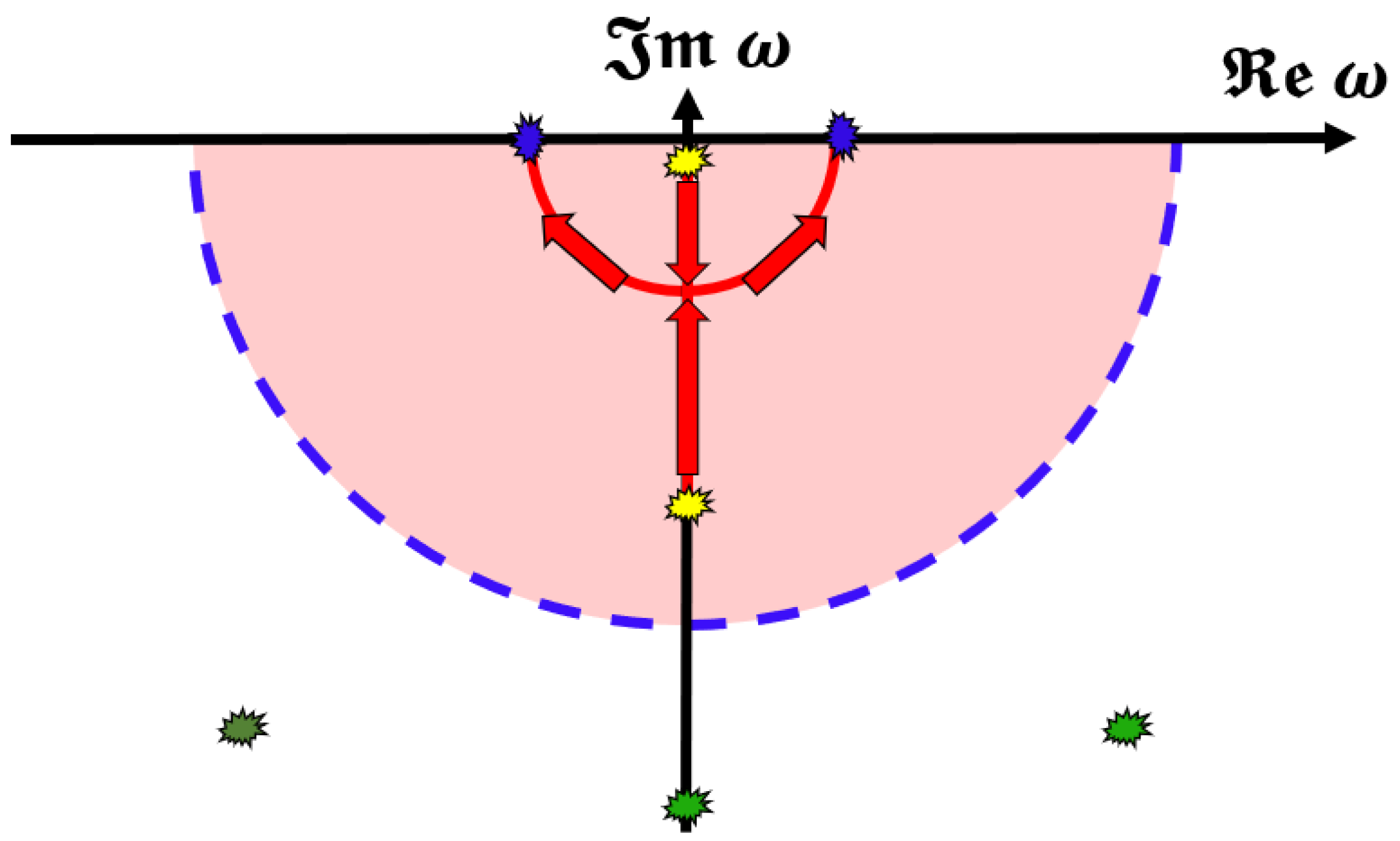
Figure 1.
Hydrodynamic frequencies of the Cattaneo model (27) when we increase D at constant k and v. For small D, there is one diffusive mode (upper yellow star) and a purely relaxing non-hydrodynamic mode (lower yellow star). As we increase D, the modes approach each other until they overlap. Then, both frequencies acquire a real part, and they travel on a circle of radius . When , the frequencies “collapse” on the real axis (blue stars), and the system becomes non-dissipative. The pink region defines the (assumed) regime of applicability of the hydrodynamic theory [53,75,76]. Outside of it, there may be infinite other dispersion relations (green stars), which are not captured by the hydrodynamic theory.

Disclaimer/Publisher’s Note: The statements, opinions and data contained in all publications are solely those of the individual author(s) and contributor(s) and not of MDPI and/or the editor(s). MDPI and/or the editor(s) disclaim responsibility for any injury to people or property resulting from any ideas, methods, instructions or products referred to in the content. |
© 2024 by the author. Licensee MDPI, Basel, Switzerland. This article is an open access article distributed under the terms and conditions of the Creative Commons Attribution (CC BY) license (https://creativecommons.org/licenses/by/4.0/).
Share and Cite
MDPI and ACS Style
Gavassino, L. Mapping GENERIC Hydrodynamics into Carter’s Multifluid Theory. Symmetry 2024, 16, 78. https://doi.org/10.3390/sym16010078
AMA Style
Gavassino L. Mapping GENERIC Hydrodynamics into Carter’s Multifluid Theory. Symmetry. 2024; 16(1):78. https://doi.org/10.3390/sym16010078
Chicago/Turabian StyleGavassino, Lorenzo. 2024. "Mapping GENERIC Hydrodynamics into Carter’s Multifluid Theory" Symmetry 16, no. 1: 78. https://doi.org/10.3390/sym16010078
Note that from the first issue of 2016, this journal uses article numbers instead of page numbers. See further details here.