Article

A Symmetrical Fuzzy Neural Network Regression Method Coordinating Structure and Parameter Identifications for Regression

Command & Control Engineering College, Army Engineering University of PLA, Nanjing 210007, China
*
Authors to whom correspondence should be addressed.
Symmetry 2023, 15(9), 1711; https://doi.org/10.3390/sym15091711
Submission received: 27 July 2023 / Revised: 21 August 2023 / Accepted: 29 August 2023 / Published: 6 September 2023
(This article belongs to the Topic Complex Systems and Network Science)

Abstract

:
Fuzzy neural networks have both the interpretability of fuzzy systems and the self-learning ability of neural networks, but they will face the challenge of “rule explosion” when dealing with high-dimensional data. Moreover, the structure and parameter identifications of models are generally performed in two stages, and this always attends to one thing and loses another in terms of interpretability and predictive performance. In this paper, a fuzzy neural network regression method (FNNR) that coordinates structure identification and parameter identification is proposed. To alleviate the problem of rule explosion, the structure identification and parameter identification are coordinated in the training process, and the numbers of fuzzy rules and fuzzy partitions are effectively limited, while the parameters of fuzzy rules are optimized. The symmetrical architecture of the FNNR is designed for automatic structure identification. An alternate training strategy is adopted by treating discrete and continuous parameters differently, and thus the convergence efficiency of the algorithm is improved. To enhance interpretability, regularized terms are designed from fuzzy rule level and fuzzy partition level to guide the model to learn fuzzy rules with simple structures and clear semantics. The experimental results show that the proposed method has both a compact structure and high precision.

1. Introduction

Fuzzy neural networks (FNNs) [1] have both interpretability and a self-learning ability, achieved by combining fuzzy systems [2,3] and neural networks, and they are important parts of the prevailing eXplainable Artificial Intelligence (XAI) field [4]. The FNN can learn a set of fuzzy IF-THEN rules with appropriate linguistic labels from data, so that it is easy to understand the decision-making process of the model. In addition, the FNN can improve its performance via an iterative algorithm. With a powerful capability for knowledge representation and learning, FNNs have been widely applied to related fields [5,6,7,8,9].
The identifications of FNNs can be divided into two parts: structure identification and parameter identification [10]. Structure identification refers to finding appropriate fuzzy partitions for the input space and determining the number of fuzzy rules. Parameter identification means determining the parameters of the antecedents and consequents of the fuzzy rules. In structure identification, the key work is to determine the number of fuzzy rules. Too many fuzzy rules will increase the complexity of the model, reduce interpretability, and easily lead to overfitting, while too few fuzzy rules will affect the performance of the model.
The adaptive network-based fuzzy inference system (ANFIS) [11] is a well-known model of FNN based on the TSK fuzzy inference system [2]. The traditional ANFIS uses the grid-based method for structure identification, that is, for features of size M, the number of fuzzy rules is M H when the fixed H-grid method is used. In terms of parameter identification, the gradient descent method, the least square method, or a combination of both is adopted by the ANFIS. For ANFIS and its variant models [11,12,13], the number of fuzzy rules is usually fixed so that the number of rules can be very large for data with high characteristic dimensions.
To alleviate “rule explosion”, some examples from the literature [14,15] transfer input variables to a new feature space in advance by feature dimension reduction, such as the principal component analysis (PCA), and then carry out the structure and parameter identifications in this new space. For example, [15] restricts the maximum feature dimension to five and utilizes the PCA if the feature number exceeds five. Some studies [16,17,18,19,20] use methods based on clustering, such as fuzzy c-means (FCM) [21], Gustafson–Kessel clustering [22], and k-nearest neighbor clustering (KNN), to obtain a small number of fuzzy rules and then use local search methods, such as the gradient descent method, linear least square method (LLS), Levenberg–Marquardt (LM) method, extreme learning machine (ELM), and so on, to adjust the parameters. For example, [17] proposes a fuzzification method for the FNN based on Bayesian clustering. In that paper, a fuzzification technique based on the concepts of FCM is used, but with a Bayesian approach to optimize the assignment processing. For methods based on clustering, the clustering number often needs to be determined in advance. Considering that the clustering number has a great impact on the performance and interpretability of the model, some studies [23,24,25] utilize cross-validation or clustering validity indicators to determine it, but this is limited in effectiveness [26]. How to interpret the obtained clustering is also an essential problem. It has been pointed out that the fuzzy partitions obtained through clustering may overlap and lack semantics [27]. Some studies [28,29] remove redundant and unnecessary rules through rule reduction and rule pruning to reduce the number of rules to a certain extent. For example, a growing-and-pruning algorithm (GP) is proposed in the literature [29]. In GP, new rules are added, and useless rules are eliminated through a sensitivity analysis of the model output. Some works [30,31] alleviate the problem of rule explosion by using a hierarchical structure. For example, [30] proposes a novel hierarchical hybrid FNN to represent systems with mixed-input variables. Several fuzzy sub-systems on the lower level randomly aggregate several discrete input variables into intermediate outputs, and a neural network whose input variables consist of continuous input variables and intermediate variables is the higher layer, thereby reducing the input dimension and the number of fuzzy rules. However, there is no general approach to selecting suitable discrete features for combination.
In the studies of FNNs, structure and parameter identifications are usually carried out separately, that is, the numbers of fuzzy rules and fuzzy partitions are determined first, and then the parameters of the rules are adjusted. Parameter identification is generally divided into two stages: the adjustment of antecedent parameters and the adjustment of consequent parameters, and different methods are selected according to the characteristics of these two parameters. This learning strategy has the advantage of low time complexity, but it cannot capture the internal correlation of various parameters and so it is difficult to find the optimal solution in the whole parameter space. To coordinate structure identification and parameter identification, meta-heuristic search methods such as particle swarm optimization algorithms and evolutionary algorithms are considered in some of the literature [32,33,34]. In these algorithms, all parameters to be learned, such as the number of rules and parameters of membership functions (MFs), are simultaneously encoded into a long and complex chromosome for joint optimization. For example, a self-organizing FNN based on the genetic algorithm is proposed in the literature [33], and a hybrid algorithm based on genetic algorithms, backpropagation, and recursive least square estimation is adopted to adjust all parameters, including the number of fuzzy rules. Moreover, the multi-objective evolutionary algorithm is regarded as a cooperative method for structure identification and parameter identification, and it has been used to construct FNNs with high prediction accuracy and a simple structure [35,36]. However, these meta-heuristic search methods have high requirements for memory and computing resources.
Based on the previous study [37], a fuzzy neural network regression method (FNNR) with high precision and a compact structure is proposed. Compared with traditional FNNs, the proposed FNNR changes the structure and training mode of the network so that the number of fuzzy rules and the number of fuzzy partitions can be limited effectively by the gradient descent method, thereby alleviating the problem of rule explosion. In the FNNR, the optimization of all parameters, including the fuzzy partition number, the fuzzy rule number, parameters of antecedents, and consequent parameters, is incorporated into the training process, and these parameters are adjusted synergistically by the gradient descent method. On this basis, the alternate training strategy is designed and utilized for different types of parameters to help the algorithm converge to the global optimal solution. To further enhance the interpretability, regularization terms are designed from fuzzy rule level and fuzzy partition level to guide the model to realize high precision with a simple structure and clear semantics. By comparisons with some representative regression models based on fuzzy rules and the classical regression method, it is proven that the proposed FNNR can achieve high prediction accuracy with high interpretability.
The main contributions are as follows:
  • A new structure and training mode of the FNN is designed for regression problems, and thus the numbers of fuzzy rules and fuzzy partitions can be learned automatically by the gradient descent method, thereby eliminating the implicit relationship between the number of rules and the number of features and fuzzy partitions, meanwhile effectively alleviating the problem of rule explosion.
  • The structure and parameter identifications of the FNN are considered as a whole, which means that the number of fuzzy partitions, the number of fuzzy rules, the MF parameters of antecedents, and the parameters of the consequent are adjusted and tuned at the same time. On this basis, an alternate training strategy is designed to help with the algorithm convergence and find the optimal solution in the whole parameter space without any pre-processing or post-processing.
  • The interpretability of the model is measured from both the fuzzy rule level and fuzzy partition level, and the measurement is introduced to the training process in terms of regularization. Therefore, the trained model has high precision with a simple structure and clear semantics.
The remainder of this paper is organized as follows. The TSK fuzzy rules and the definition of the fuzzy neural network classifier (FNNC) that we studied earlier are introduced in Section 2. In Section 3, the methodology of the FNNR is proposed. Section 4 discusses the experimental results of the comparisons of the proposed FNNR with other benchmark methods. Conclusions and future works are offered in Section 5.

2. Preliminaries

2.1. The TSK Fuzzy Rules

The Takagi–Sugeno–Kang (TSK) fuzzy system proposed by Takagi, Sugeno, and Kang [2] is one of the most famous fuzzy systems with a simple structure and a good nonlinear approximation ability. For a TSK fuzzy system with multiple inputs and a single output, the form of fuzzy rules is shown in Equation (1):
Rule   R k : if   x 1   i s   A 1 k   and   and   x M   is   A M k , then   y ¯ k = p 0 k + p 1 k x 1 + + p M k x M
where R k denotes the kth rule, and k = 1 , , K . x m represents the mth input fuzzy variable (feature), and m = 1 , , M . A m k = { < x , μ A m k ( x ) > | x U } is the fuzzy set of x m , and U [ 0 , 1 ] . μ A m k : [ 0 , 1 ] [ 0 , 1 ] denotes the MF of A m k , y ¯ k is the consequent output of R k , and p m k represents the linear function coefficients of the consequent. The “and” is the connective of the rule. The antecedents of the fuzzy rule can also be connected by the connective “or”, which can be realized by simply replacing the “and” with the “or” in Equation (1).
For the sample data d = ( x , y ) , the fuzzy reasoning method of the TSK fuzzy system is shown below:
(1)
Calculate the firing strength. The firing strength f k of the feature vector x on R k shown in Equation (1) is calculated as follows:
f k = μ A 1 k ( x 1 ) μ A M k ( x M )
where represents the fuzzy intersection operator (T-norm operator). If the connective is “or”, you just need to change the fuzzy intersection operator of Equation (2) to the fuzzy union operator (S-norm operator), which is expressed by .
(2)
Calculate the normalized firing strength. The normalized firing strength f ˙ k of the feature vector x on R k is calculated as follows:
f ˙ k = f k / k = 1 K f k
(3)
Calculate the output. The output y ¯ of the feature vector x on K fuzzy rules is calculated as follows:
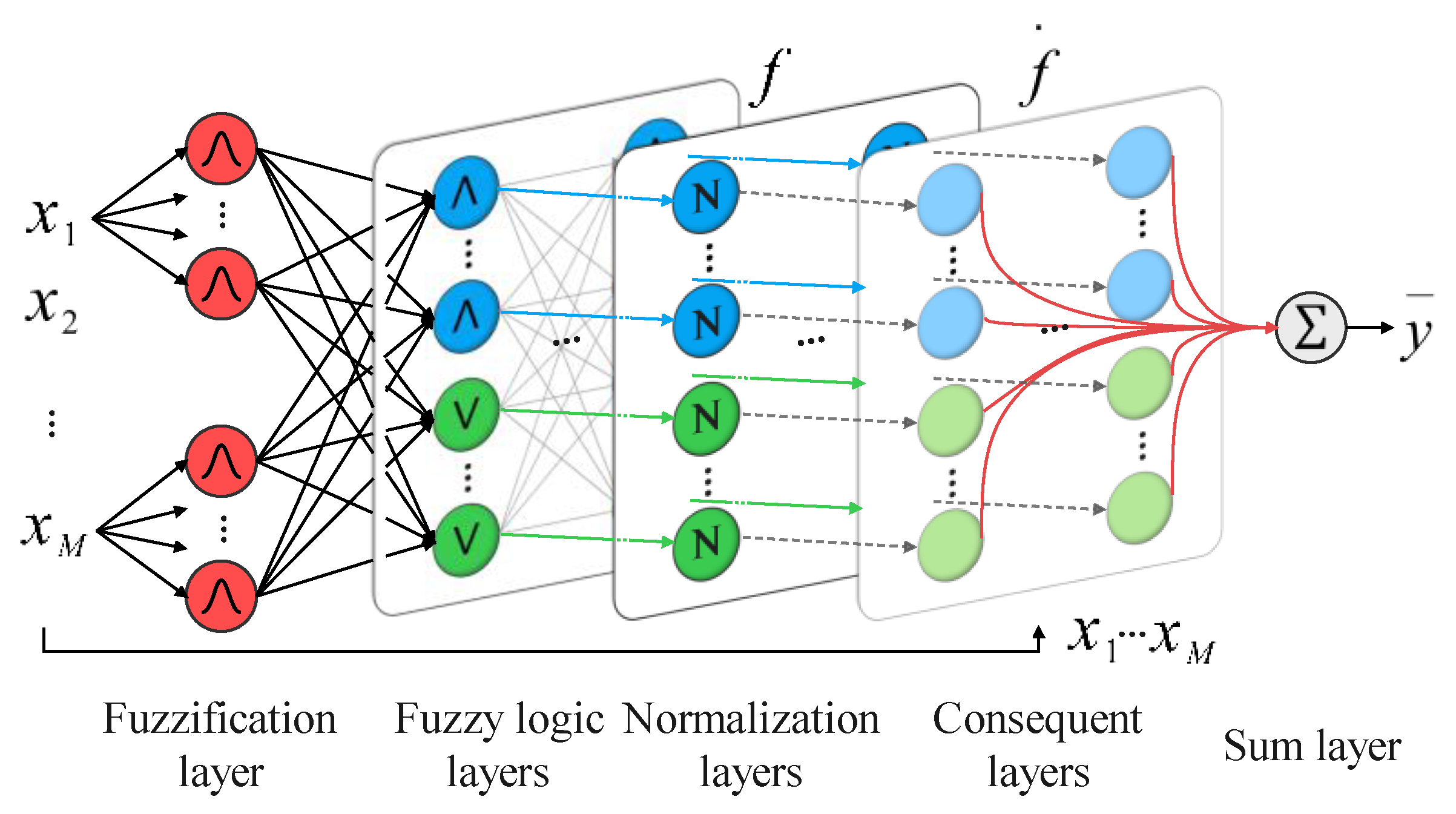
y ¯ = k = 1 K f ˙ k y ¯ k

2.2. The FNNC

The FNNC consists of three different layers: the fuzzification layer, the fuzzy logic layer, and the classification layer.
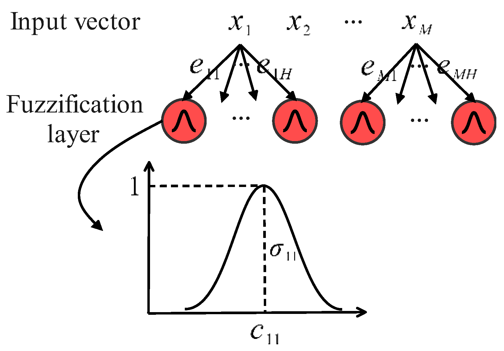
  • The fuzzification layer is utilized to translate crisp input features into fuzzy variables. Gaussian MFs are utilized. The parameters of Gaussian MFs are determined based on experience before the training and remain unchanged during the training.
  • The fuzzy logic layers are used to represent fuzzy rules. Let r i j { 0 , 1 } denote the parameter of fuzzy logic layers, where j is the jth node of the fuzzy logic layer, and i is the ith node of the previous layer (the same below). The nodes of fuzzy logic layers represent “and” and “or” connectives in fuzzy rules through fuzzy intersection operators and fuzzy union operators. Through the connecting and stacking of multiple fuzzy logic layers, complex fuzzy rules can be represented.
  • The classification layer is for integrating the outputs of fuzzy logic layers and giving the final classification. The number of nodes in the classification layer is the same as the number of class labels.
To perform structure and parameter identifications through the iterative algorithm of the neural network, the FNNC-d, the symmetrical structure of the FNNC is designed. The difference between the two lies in the parameters of fuzzy logic layers. In the FNNC-d, the parameters of fuzzy logic layers denoted by r ^ i j are continuous real numbers, i.e., r ^ i j [ 0 , 1 ] . The two parameters can be converted by the function q : [ 0 , 1 ] { 0 , 1 } :
q ( r ^ i j ) = r i j = 0 r ^ i j 0.5 1 r ^ i j > 0.5
On this basis, a parameter conversion method during the training process is designed. The FNNC can be utilized for training, testing, and interpreting, while the FNNC-d is only used for training. The gradient-updating formula of the FNNC is shown in Equation (6):
θ t + 1 = θ t η L ( Y ¯ ) Y ¯ ( Y ^ ) θ t
where θ t represents the parameter of the FNNC-d at step t, η is the learning rate, and L ( ) is the loss function. Y ¯ and Y ^ refer to the outputs of the FNNC and the FNNC-d, respectively.

3. The FNNR

In this chapter, a novel regression method of FNN named FNNR is proposed. In the FNNR, the structure identification and parameter identification are completed cooperatively, which gives the model high prediction accuracy with a simple structure and clear semantics.

3.1. The Structure of the FNNR

The structure of the FNNR is shown in Figure 1. The model consists of five different layers: the fuzzification layer, fuzzy logic layers, normalization layers, consequent layers, and the sum layer. Each layer contains several neurons, and the neurons are connected by edges.
Let L denote the layer number of the FNNR, where L = 1 + G + G + G + 1 . G is the layer number of fuzzy logic layers and G 1 . The first layer is the fuzzification layer for translating crisp input features into fuzzy variables. The middle G layers are fuzzy logic layers (same as the fuzzy logic layers in the FNNC). The nodes “ ” and “ ” refer to the fuzzy intersection operator and the fuzzy union operator, respectively, and the output of each node is the firing strength f k of the corresponding rule. The first fuzzy logic layer accepts the outputs of the fuzzification layer as the inputs, and the multiple fuzzy logic layers represent complex fuzzy rules by connecting with each other. The number of nodes “ ” and “ ” in each fuzzy logic layer and the layer number (G) can be determined according to the complexity of the task. Skip connections are added between fuzzy logic layers to conveniently express concise rules. The subsequent G layers are normalization layers for normalizing the firing strength f k output by the node in fuzzy logic layers. The next G layers are consequent layers for representing and calculating the consequent outputs of TSK rules. The last layer is the sum layer, which is used to calculate the final prediction. The normalization layers, consequent layers, and the sum layer are collectively called output layers.
The FNNR is a novel FNN model. In terms of form, like the neural network, the FNNR is composed of multi-layer neurons. The knowledge is acquired from the sample data and parameters are adjusted through training. In terms of the calculation process, the FNNR equals a TSK fuzzy system that can learn automatically. By designing the functions of different nodes, the superpositions of neurons between layers are transformed into the fuzzy logic operation, the fuzzy rule combination, and the fuzzy reasoning. Therefore, the training process of the FNNR is the process of structure and parameter identifications of the TSK fuzzy system. The key details of the FNNR are introduced in detail below.

3.1.1. The Fuzzification Layer

The fuzzification layer is utilized to translate the crisp input feature vector x = ( x 1 , , x M ) into fuzzy linguistic variable values (fuzzy sets). Let H denote the number of MFs of each feature, then there are M × H nodes in the fuzzification layer. The node of the fuzzification layer is represented by A m h , which refers to the hth fuzzy set of x m , m = 1 , , M , and h = 1 , , H . The Gaussian MFs are used to represent the fuzzy sets. To improve the prediction accuracy, the parameters of Gaussian MFs are adjusted during the training. In addition, considering that different features may use different fuzzy partitions, an additional fuzzy partition parameter, e m h { 0 , 1 } , is introduced, which refers to whether the hth fuzzy set of x m is retained: e m h = 1 means keeping the hth fuzzy set, otherwise, the hth fuzzy set is discarded. Therefore, the output of the node A m h is shown in Equation (7):
μ A m h ( x m ) = e m h exp ( ( x m c m h ) 2 2 σ m h 2 )
where μ A m h ( x m ) [ 0 , 1 ] refers to the fuzzy value of x m on the fuzzy set A m h , and c m h and σ m h are the mean and standard deviation of the Gaussian MF, respectively. The parameters of the fuzzification layer are shown in Figure 2.
It should be noted that the introduction of the fuzzy partition parameter e m h can not only control the number of fuzzy sets used for each feature but can also indirectly control the number of input variables. Specifically, when the fuzzy partition parameters corresponding to x m are all zeros, that is, e m 1 = 0 , , e m H = 0 , then x m is equivalent to being discarded and has no contribution to the prediction result.
To enable e m h , a discrete parameter, to be trained by the gradient descent and the back propagation algorithm, the FNNR-d is designed as the symmetrical model of the FNNR, and the fuzzy partition parameter of the FNNR-d, e ^ m h , is set to the continuous value of the real-value range of [0, 1]. The same as Equation (5), e ^ m h and e m h can be transformed by the function q ( ) :
q ( e ^ m h ) = e m h = 0 e ^ m h 0.5 1 e ^ m h > 0.5
The FNNR and the FNNR-d share the parameters of Gaussian MFs in the fuzzification layer.

3.1.2. The Output Layers

The output layers consist of normalization layers, consequent layers, and one sum layer. They are used to integrate the outputs of nodes in fuzzy logic layers and give the final prediction result. Let K donate the number of nodes in the fuzzy logic layers.
The normalization layer is used to normalize the firing strengths. As shown in Figure 1, normalization layers accept the firing strength f k output by the node in fuzzy logic layers and get the normalized firing strength f ˙ k , which corresponds to Equation (3), and k = 1 , , K . From Figure 1, the number of nodes in normalization layers is the same as that in the fuzzy logic layers, and there is a corresponding relationship between the normalization node and the fuzzy logic node.
The consequent layer is for computing the consequent output y ¯ k of each rule. As can be seen from Figure 1, the layer number of consequent layers is the same as that of the fuzzy logic layers, and their nodes correspond one by one. Each node of consequent layers accepts the feature vector x 1 , , x M as the input (see the arrow at the bottom of Figure 1) and calculates the consequent output y ¯ k of the corresponding rule according to Equation (9):
y ¯ k =   p 0 k + p 1 k x 1 + + p M k x M
Therefore, the parameters of consequent layers are the linear function coefficients of TSK rules, which are denoted by W P .
The sum layer is used to integrate the normalized firing strength f ˙ k and the consequent output y ¯ k of each rule to obtain the final prediction. The normalization layers pass f ˙ k to consequent layers (see the gray arrow in Figure 1). Then, consequent layers take f ˙ k together with the output y ¯ k as the inputs of the sum layer and, finally, the summation operation is complete in the sum layer, which corresponds to Equation (4). It should be noted that the normalization layers and the sum layer have no trainable parameters, and they only complete the normalization operation and the summation operation, respectively. Therefore, the parameter scale of output layers is M K , where M is the number of input features, and K is the number of nodes in fuzzy logical layers.
Since the trainable parameters ( W P ) of output layers are values of the continuous interval, the FNNR and the FNNR-d share the output layers.

3.2. Training

3.2.1. The Design of the Loss Function

Similarly to the FNNC, the FNNR needs to find the gradient direction with the help of its symmetrical model, FNNR-d, thus the updating of parameters is similar to Equation (6), except that the loss function is different. For the FNNR, since the structure identification and parameter identification are coordinated, there are altogether four kinds of parameters that need to be trained through gradient descent algorithm, which are the parameters of Gaussian MFs, W G ( c , σ ) , the fuzzy partition parameters, W E ( e ) , the parameters of fuzzy logic layers, W R ( r ) , and the consequent parameters, W P ( p ) . The change in these parameters will not only influence the prediction accuracy of the model but also greatly affect its interpretability. Therefore, the loss function is divided into two parts: L a c c ( ) and L i n t e r ( ) , which are utilized to calculate the loss of prediction accuracy and interpretability, respectively.
The loss function of the prediction accuracy L a c c ( ) is calculated as shown in Equation (10):
L a c c ( Y ¯ ) = MSE ( Y , Y ¯ ( X , W ) )
where the mean square error (MSE) function is used. W = ( W G , W P , W E , W R ) represents the parameters of the FNNR, including parameters of Gaussian MFs ( W G ), consequent parameters ( W P ), discrete parameters of fuzzy partitions ( W E ), and discrete parameters of fuzzy logic layers ( W R ). Y ¯ is the output of the FNNR, which is the final prediction, and Y is the label.
The measure of the model’s interpretability is considered from two levels: the interpretability at the fuzzy rule level and the interpretability at the fuzzy partition level as shown in Table 1. Among them, the fewer rules extracted from the model and the fewer antecedents of the rule, the more concise and explainable fuzzy rules are. The fewer input variables and MFs the model uses and the more complementary the fuzzy partition is, the clearer the fuzzy partition is and the more interpretable the model is. Here, the complementarity [38] refers to the fact that the sum of the fuzzy values of input features on all fuzzy partitions is close to one.
Therefore, the loss function L i n t e r ( ) that measures the interpretability of the FNNR is revealed in Equation (11):
L i n t e r ( W ^ ) = λ 1 φ 1 ( W G ) + λ 2 | | W ^ E | | 2 2 + λ 3 | | W ^ R | | 2 2
where W ^ = ( W G , W P , W ^ E , W ^ R ) are parameters of the symmetrical model FNNR-d. λ 1 , λ 2 , and λ 3 are the regularization coefficients for parameters of Gaussian MFs ( W G ), parameters of fuzzy partitions ( W ^ E ), and parameters of fuzzy logic layers ( W ^ R ), respectively. φ 1 ( ) is the function that measures the complementarity of fuzzy sets as shown in Equation (12):
φ 1 ( W G ) = x ( h = 1 H μ A h ( x ) 1 ) 2
where x is the value of the input feature, A h refers to the hth fuzzy set of x, and H is the fuzzy set number of x.
It can be observed from Equation (11) that the first item of L i n t e r ( ) can help to enhance the complementarity of fuzzy partitions during the training, the second item can help the model to reduce the number of input variables and MFs in the training process, and the third item can help to reduce the number of fuzzy rules and antecedents in the training process.
In conclusion, the formula of parameter updating is shown in Equation (13):
w ^ t + 1 = w ^ t η ( L a c c ( Y ¯ ) Y ¯ ( Y ^ ) w ^ t + L i n t e r ( w ^ t ) w ^ t )
where w ^ W ^ represents the parameter of the symmetrical model FNNR-d. Y ¯ and Y ^ are the outputs of the FNNR and the FNNR-d, respectively.

3.2.2. The Alternate Training Strategy

As mentioned above, the FNNR and its symmetrical model FNNR-d contain four types of trainable parameters, where parameters of Gaussian MFs W G and consequent parameters W P are shared, while parameters of fuzzy partitions and fuzzy logic layers are different, which can interchangeable by q ( ) (see Equations (5) and (8)). According to q ( ) , when the values of fuzzy partition parameters W ^ E and fuzzy logic layer parameters W ^ R in the FNNR-d cross 0.5, the corresponding discrete fuzzy partition parameters W E and fuzzy logic layer parameters W R in the FNNR will jump from 0 to 1 (or from 1 to 0), and then the parameters of Gaussian MFs W G and the consequent parameters W P will change dramatically. Therefore, when the above four kinds of parameters are trained together, we find that the model is difficult to converge during the training process: W ^ E and W ^ R oscillate around 0.5, which leads to the constant oscillation of W G and W P , making it difficult to find the optimal solution. To solve this problem, an alternate training strategy is designed and adopted in training as shown in Algorithm 1.
Algorithm 1: Alternate Training Strategy.
input: The dataset, D ; the number of epoches for joint training, E 1 ; the number of epoches for fixing fuzzy logic layers, E 2 ; the number of epoches for fixing fuzzy partitifon parameters, E 3 .
output: A trained FNNR model, FNNR
begin
   initialize the parameters of model
   for  i < v  do
     training and updating all the parameters with D for E 1 epoches\;
     training and updating all the parameters except for W ^ R with D for E 2 epochs;
     training and updating all the parameters except for W ^ E with D for E 3 epochs;
      i = i + 1 ;
   end
   return FNNR
end
It can be observed from Algorithm 1 that the whole training cycle is divided into v rounds and each round is divided into three stages: the stage of joint training, the stage of fixed fuzzy logic layers, and the stage of fixed fuzzy partition parameters. Utilizing three stages of alternate training, the problem of the model brings difficult to converge, caused by the oscillation of fuzzy partition parameters and fuzzy logic layer parameters, can be alleviated.

4. Experiments

To verify the regression performance of the proposed method, the FNNR is compared with the representative regression methods, based on fuzzy rules proposed recently, and the classical regression algorithm on benchmark datasets.

4.1. Experimental Design

We have the following questions in mind while designing and conducting the experiments:
(1)
How does the FNNR perform when compared with other state-of-the-art regression methods?
(2)
What roles do the training modes of the fuzzification layer, the design of the output layers, and the strategy of alternate training play in the FNNR?
(3)
How much do different regularization coefficients affect the final prediction of the FNNR?
(4)
How explainable is the FNNR?
To answer (1), we compare the performance of the FNNR with several benchmark methods. To answer (2), we conduct some ablation studies on the proposed model. To answer (3), we change the regularization coefficients to make comparisons. To answer (4), the fuzzy rules used by the FNNR to make predictions are visually displayed on two datasets.

4.1.1. Datasets

A total of 28 real regression datasets are selected from KEEL [39] repository as baseline datasets. These datasets have different feature numbers (from two to forty) and sample numbers (from 337 to 40,768). According to the dimension of features, these 28 datasets are divided into two categories: 11 low-dimensional datasets and 17 high-dimensional datasets. Supplementary S1 shows detailed information on the two types of datasets. For the low-dimensional datasets, the number of features is small (all less than seven), and the number of samples is also relatively small, which is up to 4052, so the regression tasks on low-dimensional datasets are relatively simple. For high-dimensional datasets, the number of features is large, especially for the last four datasets, and the feature numbers are all over 20. Considering that fuzzy rules are better at fitting data with small feature dimensions [14], the regression performance of the model is challenged. In addition, in high-dimensional datasets, some of them have small sample sizes, such as FOR and BAS, which increases the risk of overfitting. Finally, there are quite a few datasets with large sample sizes, such as CAL, MV, and HOU, which may consume a lot of computing resources.

4.1.2. Parameter Settings for the FNNR

In the FNNR, Gaussian MFs used in the fuzzification layer are set as the uniform MFs in the domain [0, 1], that is, the mean vector of Gaussian functions is shown in Equation (14):
c = ( 0 , 1 ) H = 2 ( 0 , 1 / ( H 2 ) , 1 ) H = 3 ( 0 , 1 / ( H 2 ) , 2 / ( H 3 ) , , 1 ) H > 3
Each MF uses the same standard deviation: σ = 2 ( 1 / H ) 2 . Fuzzy partition parameters are all initialized to 1 s. To enhance the model interpretability as much as possible, the initial number of fuzzy sets for each feature, H, is set to seven. Considering that the prediction task on low-dimensional datasets is relatively simple, parameters of MFs and fuzzy partitions in the FNNR on low-dimensional datasets are fixed and unchanged with H   { 3 , 5 } . The number of fuzzy logic layers is chosen from { 1 , 2 } . Depending on the regression difficulties of different datasets, the number of nodes in each fuzzy logic layer ranges from two to fifty. We utilize the Adam method and the MSE loss function for the training process. The round number v for the alternate training strategy is set to three, and the cycle numbers of three training stages are set to 100 in each round, i.e., E 1 , E 2 , E 3 = 100 . The ranges of regularization coefficients in Equation (11) are as follows: λ 1 { 0 , 1 × 10 4 , 1 × 10 2 , 1 } , λ 2 { 1 × 10 3 , 1 × 10 6 , 1 } , and λ 3 { 1 × 10 2 , 1 × 10 4 , 1 × 10 6 , 1 × 10 8 , 1 × 10 10 } . The min-max normalization is carried out on features and labels. For a fair comparison, the prediction results of the proposed method are inversely normalized and the MSEs with the original labels are calculated and recorded.

4.1.3. Experimental Settings

  • Benchmark Methods
To evaluate the regression performance of the proposed FNNR, it is compared with some representative regression methods based on fuzzy rules and one classical regression algorithm, including the following seven methods:
    • The decision tree (DT) [40];
    • The training algorithm for the TSK fuzzy system based on mini-batch gradient descent with regularization, droprule, and adabound (MBGD-RDA) [14];
    • The learning algorithm of TSK fuzzy rules based on evolutionary learning (FRULER) [41];
    • The learning algorithm of the TSK fuzzy system based on multi-objective evolutionary algorithms (METSK-HD) [35];
    • The learning algorithm of the zero-order TSK fuzzy system based on Apriori and local search methods (Freq-SD-LSLS) [42];
    • The learning algorithm of Mamdani fuzzy rules based on multi-objective evolutionary learning algorithms (MOKBL + MOMs) [36];
    • Disjunctive fuzzy neural network (DJFNN), a new splitting-based approach to designing a TS fuzzy model [10].
The experimental results of the benchmark methods are directly cited from [10].
  • Evaluation Metrics
In this paper, the MSE on the test dataset is adopted to evaluate the regression performances of different methods, which is shown in Equation (15):
M S E = 1 2 N t e s t n = 1 N t e s t ( y ¯ n y n ) 2
where N t e s t is the sample size of the test data. y ¯ n and y n refer to the prediction and the label of the nth sample, respectively. In this paper, all the experiments are repeated 10 times on each dataset, and the average MSEs are reported.
  • The Significance Testing
To further explore whether the observed differences are statistically significant, the Friedman test [43] for multiple comparisons and the Bonferroni–Dunn post hoc test [44] to identify pairwise differences are applied.

4.2. Result Analysis

The average ranks (AvgR) and average MSEs of the proposed FNNR and the other four regression methods on low-dimensional test data are reported in Table 2, where the results of ELE1, DELAIL, and DELELV should be multiplied by 10 5 , 10 8 , and 10 6 (the same below). The minimum MSE on each dataset is highlighted in bold.
We can conclude from Table 2 that:
1.
The proposed FNNR achieves the minimum average MSEs on seven of eleven datasets among the models involved. On three of the remaining four datasets, FNNR still exhibits the second-best performance. It proves that the proposed FNNR method has a significant performance advantage on low-dimensional and simple tasks. Considering that parameters of MFs and fuzzy partitions in the fuzzification layer are not adjusted during the training process on low-dimensional datasets, there is still a lot of room for performance improvement of the FNNR.
2.
The FNNR shows great improvement over the other four approaches in terms of regression performance. On some datasets, such as ELE1, FRIE, and MPG8, the FNNR reduces the MSEs by over 20% compared with the recently proposed DJFNN. Moreover, the average MSEs are more than 4% lower than the DJFNN on datasets ELE2 and MPG6.
3.
The significance tests are conducted on the results shown in Table 2. The Friedman test suggests rejecting the H 0 hypothesis ( F F = 5.825 > 2.091 ) for a significance level of 0.1 with (4, 40) degrees of freedom. This suggests that on low-dimensional datasets, there are significant differences between at least two methods across the benchmark. The Bonferroni–Dunn post hoc test suggests that the regression performance of the FNNR is significantly different from that of DT, MBGD-RDA, and FRULER, while the performance of the FNNR and the DJFNN are equivalent.
The average ranks and average test MSEs of the proposed FNNR and all of the seven regression methods on high-dimensional datasets are reported in Table 3, where the results of CAL, BAS, HOU, ELV, PUM, and AIL should be multiplied by 10 9 , 10 5 , 10 8 , 10 6 , 10 4 , and 10 8 (the same below). The minimum MSE on each dataset is highlighted in bold.
We can conclude from Table 3 that:
1.
The FNNR also shows great improvement over other approaches in terms of regression performance on high-dimensional tasks. On some datasets, such as STP, MV, and POLE, the FNNR reduces the errors by about 50% compared with the DJFNN. Moreover, the average MSEs are more than 20% lower than the DJFNN on datasets CON, MOR, and CA.
2.
The proposed FNNR obtained the minimum MSEs on the last four datasets with high feature dimensions, which indicates that the selection of features and antecedents is completed flexibly through trainable parameters of fuzzy partitions and fuzzy logic layers in the FNNR. For datasets BAS and FOR, which are easy to overfit, although the FNNR does not get the optimal performance among all the methods, there is no significant difference between the average error of the FNNR and the best one, with increases of 2% and 10.8%, respectively. It indicates that the proposed method can avoid overfitting to a certain extent. On datasets with large sample sizes like MV, CAL, and HOU, the FNNR achieves the minimum MSEs, showing that the FNNR also has good performance in handling regression tasks with large samples.
The Friedman test suggests rejecting the H 0 hypothesis ( F F = 20.024 > 1.771 ) for a significance level of 0.1 with (7112) degrees of freedom. This suggests that there are significant differences between at least two methods across the benchmark. The Bonferroni–Dunn post hoc test suggests that the regression performance of the FNNR is significantly different from that of the DJFNN ( 1.412 > C D α = 1.188 ).

4.3. Ablation Study

To illustrate the functions and effects of some key technologies in the FNNR, such as the training modes of the fuzzification layer, the design of the output layers, and the alternate training strategy, ablation studies are carried out. For fairness, the rest of the parts remain unchanged and the hyperparameters remain the same during ablation experiments.

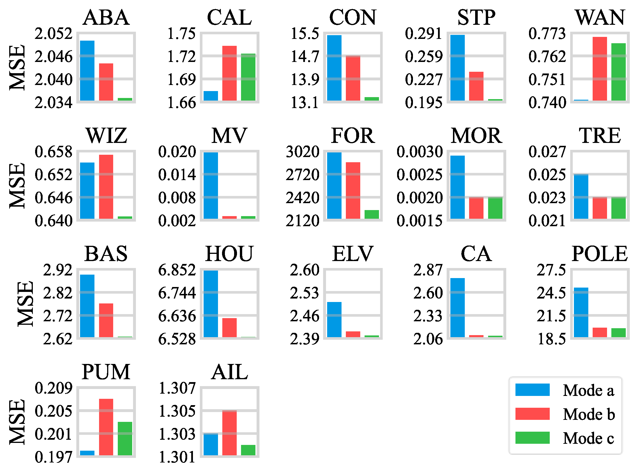
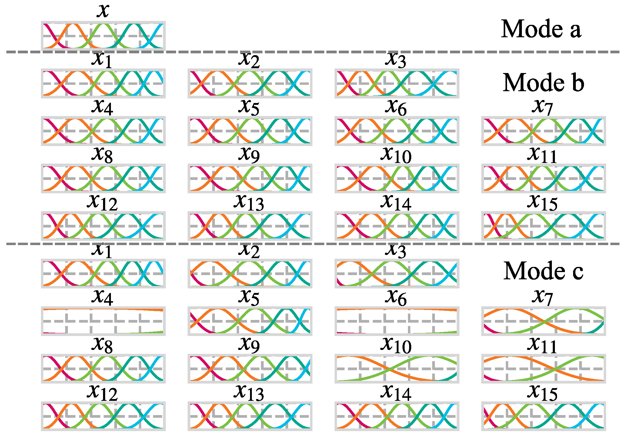
4.3.1. The Ablation of Training Modes of the Fuzzification Layer

To illustrate the influence of training modes of parameters in the fuzzification layer on the regression performance, the following three different training modes are adopted:
  • The parameters of the fuzzification layer are fixed during the training.
  • Only the parameters of Gaussian MFs in the fuzzification layer are trained.
  • The parameters of Gaussian MFs and fuzzy partitions in the fuzzification layer are trained together.
On high-dimensional datasets, the average prediction MSEs of the FNNR using the above three training modes are shown in Figure 3. The FNNR achieves the minimum errors on 14 of 17 high-dimensional datasets using training mode c. Compared with training mode b, the regression performance of the FNNR with training mode c is slightly improved, for example, the MSEs on datasets ABA, CON, STP, FOR, and BAS are reduced by 4% to 22%. Compared with training mode a, the performance with training mode c is greatly improved, and the MSEs on datasets CON, STP, MV, FOR, MOR, CA, and POLE are reduced by 10% to 85%.
Figure 4 reveals the fuzzy sets of each feature obtained by the above three training modes on the MOR dataset. Since the parameters of MFs are not modified and the same parameters of fuzzy partitions and MFs are used for all the features when using training mode a, the fuzzy sets of only one feature are displayed, and the fuzzy sets of the other features are the same.
As can be observed from Figure 3 and Figure 4, training mode b enhances the fitting ability and improves the performance of the model by fine-tuning the parameters of MFs, and training mode c further reduces the test error of the model by discarding unimportant fuzzy partitions.

4.3.2. The Ablation of the Rule Type Represented by the Output Layers

The output layers of the FNNR consist of normalization layers, consequent layers, and the sum layer, which complete the representation of consequents in the TSK rules and the inference of prediction together. To verify the validity and rationality of the data fitting ability using TSK fuzzy rules, an ablation study is conducted on the rule type. In this study, the TSK fuzzy rules are replaced by Mamdani fuzzy rules [3] and the fuzzy rules for using nonlinear calculations in the consequents.
(1)
The FNNR model with Mamdani fuzzy rules
Like TSK fuzzy rules, Mamdani rules are also a kind of fuzzy rule that are common and widely used. Different from the former, the antecedents and consequents of Mamdani rules are interpretable linguistic variables, so their interpretability is stronger. For convenience of representation, the original FNNR model is called FNNR-T, and the FNNR using Mamdani fuzzy rules is called FNNR-M.
The function of output layers in the FNNR-M is as the center average defuzzifier [45]. The output layers of the FNNR-M consist of one consequent layer and one sum layer, where the nodes of the consequent layer represent the fuzzy set of the output variable and the number of nodes is the fuzzy partitions number of the output variable, which is set to H M . The parameters of the consequent layer are continuous real values in the interval [0, 1] that represents the rule weights. The consequent layer is fully connected with the fuzzy logic layers, and the output of each consequent node is the weighted sum of firing strengths of the rules whose consequent is the corresponding fuzzy set. For the FNNR-M, the parameter scale in the output layers is H M K , where K is the number of nodes in fuzzy logic layers. Supplementary S2 shows more details on the FNNR-M.
(2)
The FNNR model with rules whose consequents use nonlinear calculations
Considering that the fully connected network has high prediction accuracies in regression tasks, the consequent layers of the FNNR are replaced by fully connected layers, which is called the FNNR-F. In the FNNR-F, the output layers are composed of fully connected layers and one sum layer. The layer number of fully connected layers is set as I F ( I F 1 ) , and the number of nodes for each layer is set as n F . The ReLU function is utilized as the activation function. Of course, for the FNNR-F, the prediction is the result of a complex weighted sum and nonlinear activation of the firing strengths, which reduces the model interpretability to a certain extent. The parameter scale of the output layers is I F ( n F + 1 ) + n F K . Supplementary S3 shows more details on the FNNR-F.
Table 4 shows the average MSEs of FNNR-M, FNNR-F, and FNNR-T on 28 datasets, where H M is set as five, I F is set as two, and n F is set as twenty. The minimum error on each dataset is highlighted in bold.
As can be seen from Table 4, the regression performance of the FNNR-M is the worst: it can only achieve the minimum test errors on four of twenty-eight datasets. The FNNR-F has the best regression performance and can obtain the minimum test errors on 15 datasets. The performance of FNNR-T is middle-ranking with the minimum MSEs on 11 datasets. An analysis of the time complexity of the three models is given in Supplementary S4.
To improve the prediction accuracy of the FNNR-M and reduce the complexity of FNNR-F to enhance its interpretability, ablation analyses are performed on hyperparameters H M and I F , where H M { 3 , 5 , 7 } , and I F { 1 , 2 , 3 , 4 } . Table 5 illustrates the average MSEs of the above two models under each specified hyperparameter. The minimum error of each model on each dataset is highlighted in bold.
As can be observed from Table 5, when increasing the complexity of the FNNR-M (increasing the number of nodes in the consequent layer), the regression performance cannot be significantly improved. When the number of nodes in the consequent layer is increased to seven, the minimum error can only be achieved on CAL dataset. For the FNNR-F, when the complexity is reduced (reducing the number of fully connected layers), the regression performance of the model is greatly affected. When the number of fully connected layers is reduced to one, the model can only achieve the minimum MSEs on three datasets. It is worth noting that when the complexity of the FNNR-F is increased, the performance does not get better. On the one hand, this is related to the phenomenon of vanishing gradient; when the number of fully connected layers increases, the gradient at the back of the network has difficulty being transmitted to the front layers, resulting in low learning efficiency of the parameters of the fuzzification layer and fuzzy logic layers. On the other hand, the conclusion can be drawn by the comparison of MSEs on training sets and test sets that when the number of fully connected layers increases, the risk of overfitting gradually increases.
By conducting ablation experiments on the rule type represented by the output layers, it can be concluded that neither FNNR-M nor FNNR-T can properly balance prediction accuracy and interpretability. Therefore, it is most appropriate to adopt TSK fuzzy rules in the FNNR model.

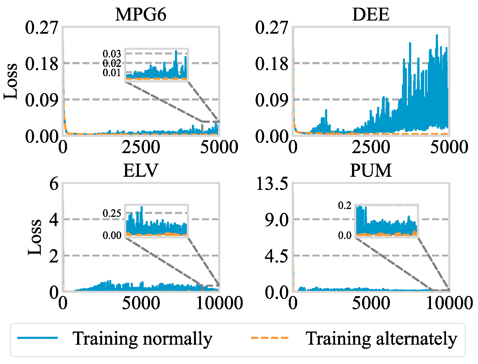
4.3.3. The Ablation of Alternate Training Strategy

As mentioned above, to avoid the problem that the model has difficulty converging due to the oscillation of fuzzy partition parameters and fuzzy logic layer parameters in the training process, a three-stage alternate training strategy is designed. To demonstrate the effectiveness of this strategy, an ablation analysis is performed.
The FNNR-T is trained using the alternate training strategy and normal training method on all 28 datasets, and the average test errors are recorded. To highlight the role of alternate training strategy, parameters of MFs and fuzzy partitions are fixed during the training, and the whole training process is only divided into two stages: the stage of joint training and the stage of the fixed fuzzy logic layer. It is found that for 24 of the 28 datasets, the average MSEs are lower when using the alternate training strategy. This indicates that the alternate training strategy can help to improve the prediction accuracy of the model. Experiments are also conducted on the other two models, and relevant experimental data and analyses are shown in Supplementary S5.
Figure 5 reveals the training loss of the FNNR-T on low-dimensional datasets MPG6 and DEE and high-dimensional datasets PUM and ELV when the alternate training strategy and normal training method are adopted. For intuition, 5000 cycles are trained on low-dimensional datasets and 10,000 cycles are trained on high-dimensional datasets. It can be observed that the loss gradually diverges in the later training period and cannot converge when adopting the normal training method, while the alternate training strategy can help the loss gradually stabilize and finally converge.

4.4. Parameter Analysis

To understand the influence of regularization coefficients on the training and regression performance of the model, parameter analyses on λ 1 and λ 2 are carried out in this chapter.

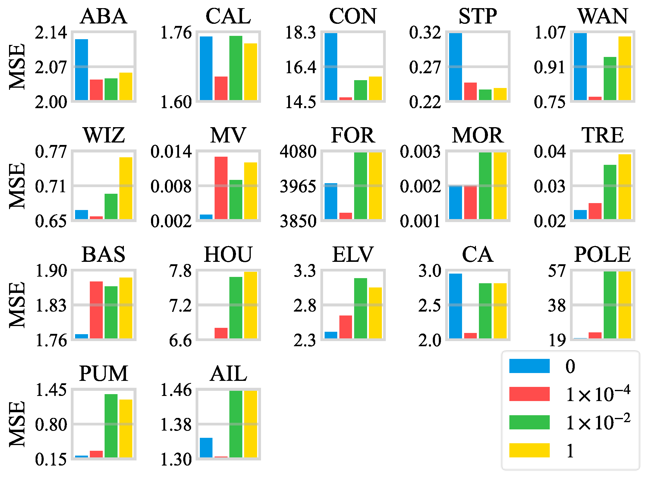
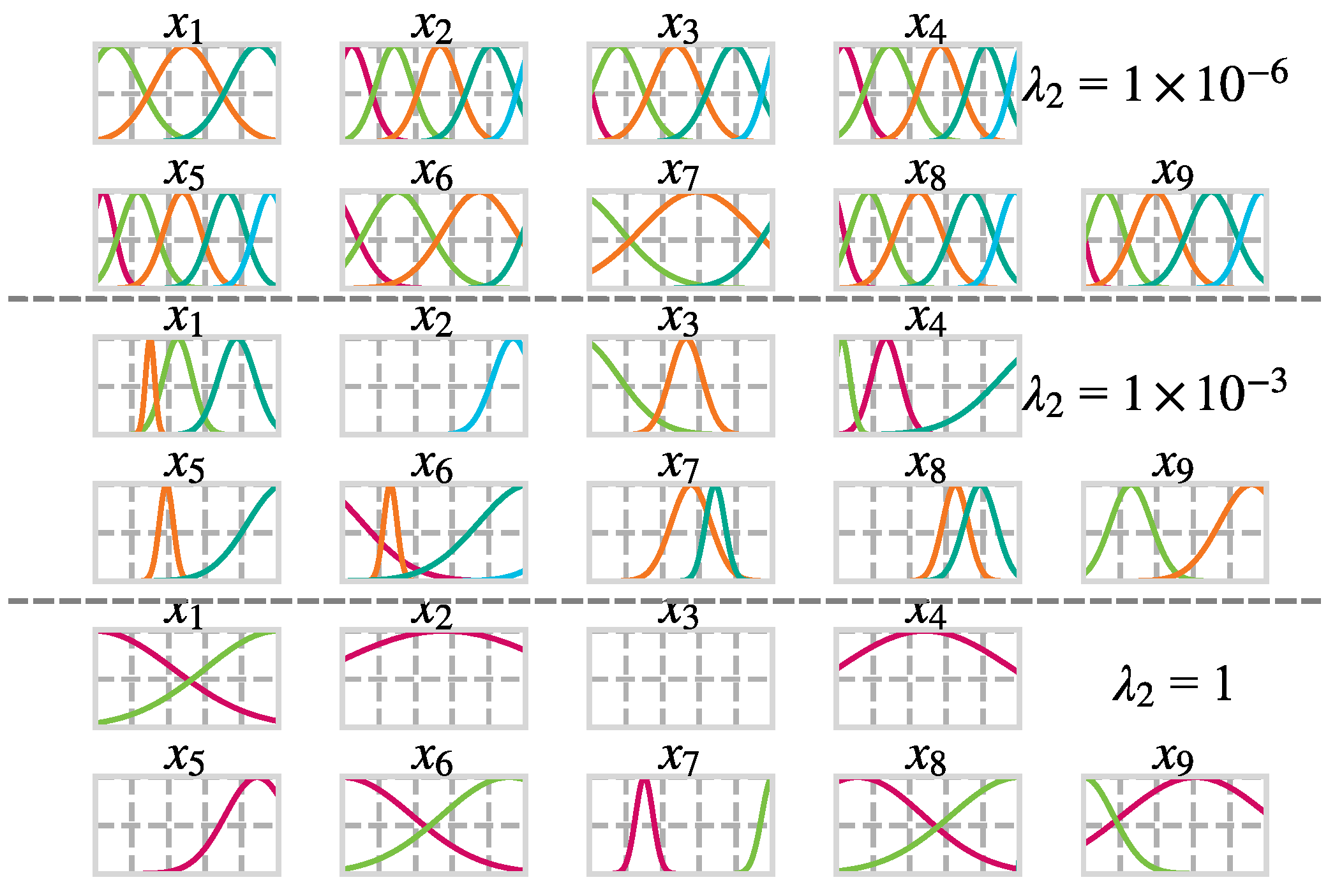
4.4.1. The Parameter Analysis on the Regularization Coefficient λ 1

Firstly, the regularization coefficient λ 1 is analyzed. As mentioned above, λ 1 is the regularization coefficient to measure the complementarity of fuzzy sets. The larger λ 1 is, the stronger the complementarity of fuzzy sets will be, the clearer the semantics of fuzzy sets will be, and the stronger the interpretability will be. Figure 6 illustrates the average prediction errors of the FNNR-T under different values of λ 1 in high-dimensional datasets. Similarly, to clearly show the influence of regularization coefficients, fuzzy partition parameters are fixed in the training process.
As can be observed from Figure 6, when λ 1 = 0 and λ 1 = 1   ×   10 4 , the model gets the minimum MSEs on eight datasets; under the circumstances of λ 1 = 1 and λ 1 = 1   ×   10 2 , the model achieves the minimum error on only one dataset. This indicates that with the increase of λ 1 , when it rises to a threshold, the regression accuracy of the model will decrease gradually. This is also in line with our subjective feelings: with the increase of the regularization coefficient, the model pays too much attention to the complementarity of fuzzy sets during training, which leads to a decrease in accuracy.
Figure 7 shows the fuzzy sets that the model eventually learns under the four values of λ 1 in the CON dataset, respectively. It can be observed that the interpretability of fuzzy sets is poor when λ 1 = 0 . Some areas are covered repeatedly by a few fuzzy sets at the same time, so the semantics is peculiarly fuzzy. For example, when x 1 is near 0.8 with λ 1 = 0 , the firing strengths of three fuzzy sets are very high, which is not intuitive. In addition, there are several fuzzy sets whose shapes are “sharp”, such as the second fuzzy set of x 2 when λ 1 = 0 , which is also poorly interpretable. With the increase of λ 1 , the fuzzy sets tend to be uniform, and the interpretability is enhanced gradually.

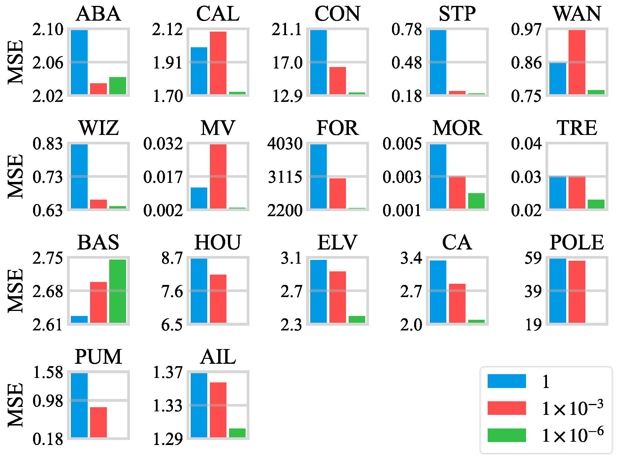
4.4.2. The Parameter Analysis on the Regularization Coefficient λ 2

The regularization coefficient λ 2 is analyzed below. λ 2 is the regularization coefficient to control the number of fuzzy sets of features. The larger λ 2 is, the fewer fuzzy sets there are, and the more explainable the model is. Figure 8 reveals the average prediction errors of the FNNR-T under different values of λ 2 on high-dimensional datasets. For the sake of fairness, λ 1 is set to 1 × 10⁻⁴.
As can be seen from Figure 8, when λ 2 = 1 × 10 6 , the model has the best regression performance, and it can reach the minimum errors on 13 of 17 datasets. When λ 2 = 1 , the regression performance of the model is poor, and it can only reach the minimum MSE on one dataset. Compared with λ 2 = 1 × 10 6 , the average errors under λ 2 = 1 increase by more than 20% on 11 datasets. When λ 2 = 1 × 10 3 , the regression performance of the model is middle-ranking, and the prediction errors are minimized on two datasets. Compared with λ 2 = 1 × 10 6 , the errors increase by more than 20% on seven datasets under λ 2 = 1 × 10 3 . The results observed above are in line with our subjective feelings: With the increase of λ 2 , the number of fuzzy partitions decreases continuously. Therefore, the remaining fuzzy sets are hard to reasonably divide in the input space, and the accuracy of the model is seriously affected.
Figure 9 illustrates the fuzzy sets finally learned by the model using different values of λ 2 on the STP dataset. From the figure, when the regularization coefficient is moderate, inappropriate fuzzy sets will be discarded, and the number of fuzzy sets used for each feature is well optimized. When the regularization coefficient is too large, many fuzzy sets are discarded, and the remaining fuzzy sets are difficult to partition in the input space reasonably and efficiently.

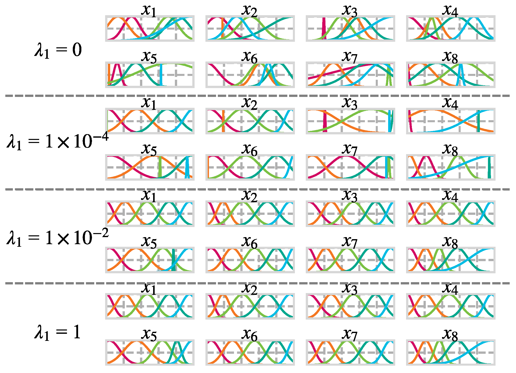
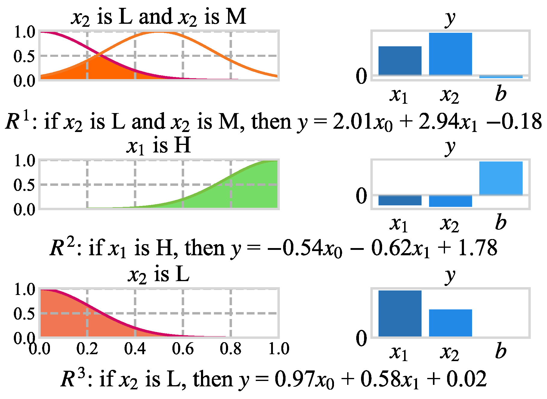
4.5. The Interpretability of the FNNR

The proposed FNNR has good interpretability, and TSK fuzzy rules can be directly extracted from the trained FNNR. The course of rule extraction is very simple: one fuzzy rule can be extracted if the node in the fuzzy logic layers whose parameter is one is found.
To visually illustrate the interpretability of the model, Figure 10 and Table 6 show the fuzzy rules extracted from the model in datasets ELE1 and MPG8, respectively, where L, M, and H are the names of fuzzy sets when the fuzzy partition number is three, and L, ML, M, MM, and H are the names of fuzzy sets when the fuzzy partition number is five. b is the constant coefficient of the consequent. As can be seen, whether the feature number is small or large, the model can achieve low regression error with a small number of rules.

5. Conclusions and Future Work

A novel explainable fuzzy neural network regression method (FNNR) is proposed in this paper. To solve the problem of rule explosion on high-dimensional datasets, the symmetrical structure and corresponding parameter transformation method are used to learn the number of fuzzy rules and fuzzy partitions automatically. In addition, the structure identification and parameter identification of the model are considered. The number of fuzzy rules, the number of fuzzy partitions, the parameters of Gaussian MFs, and the consequent parameters are trained synergistically. On this basis, an alternate training strategy is designed to train different types of parameters to promote convergence. To further enhance the interpretability of the model, the regularized items are designed from fuzzy rule level and fuzzy partition level to guide the model to learn fuzzy rules with a simple structure and clear semantics. Experimental results on datasets with low and high dimensions show that the proposed model can achieve high test accuracy with good interpretability by comparing with some representative regression methods based on fuzzy rules and the classical regression models.
First, various uncertainties that may exist in the datasets, such as missing values, error values, noises, abnormal values, and so on, are not considered in this study. Future research could combine rough sets [46] and other technologies with fuzzy sets to deal with the above uncertainties. In addition, the type-I fuzzy sets used in this paper can also be extended to type-II fuzzy sets or interval fuzzy sets [47,48] to better deal with the uncertainty in the data. Secondly, in this study, Gaussian MFs are utilized to represent the fuzzy sets of all features. Considering different MFs and their combinations or using the shape of MFs as a learnable parameter is another possible future research direction. Finally, the gradient-based method is adopted in this study to train all parameters together as a whole. This method requires no intervention, but it is time-consuming in large datasets. Learning from some fast training methods, such as pseudoinverse [49] and heuristic greedy search [10], to conduct collaborative training for various parameters is also a potential future research topic.

Supplementary Materials

The following supporting information can be downloaded at: https://www.mdpi.com/article/10.3390/sym15091711/s1.

Author Contributions

Validation, W.H.; Writing—original draft, K.Z.; Writing—review & editing, X.Y.; Supervision, T.S. All authors have read and agreed to the published version of the manuscript.

Funding

This research was funded by Defense Industrial Technology Development Program grant number [JCKY2020601B018].

Data Availability Statement

Not applicable.

Conflicts of Interest

The authors declare no conflict of interest.

References

  1. Das, R.; Sen, S.; Maulik, U. A survey on fuzzy deep neural networks. ACM Comput. Surv. 2020, 53, 1–25. [Google Scholar] [CrossRef]
  2. Kerk, Y.W.; Tay, K.M.; Lim, C.P. Monotone Fuzzy Rule Interpolation for Practical Modeling of the Zero-Order TSK Fuzzy Inference System. IEEE Trans. Fuzzy Syst. 2022, 30, 1248–1259. [Google Scholar] [CrossRef]
  3. Li, G.; Peng, C.; Xie, X.; Xie, S. On Stability and Stabilization of T–S Fuzzy Systems with Time-Varying Delays via Quadratic Fuzzy Lyapunov Matrix. IEEE Trans. Fuzzy Syst. 2022, 30, 3762–3773. [Google Scholar] [CrossRef]
  4. Arrieta, A.B.; Díaz-Rodríguez, N.; Del Ser, J.; Bennetot, A.; Tabik, S.; Barbado, A.; García, S.; Gil-López, S.; Molina, D.; Benjamins, R.; et al. Explainable artificial intelligence (XAI): Concepts, taxonomies, opportunities and challenges toward responsible AI. Inf. Fusion 2020, 58, 82–115. [Google Scholar] [CrossRef]
  5. De Campos Souza, P.V. Fuzzy neural networks and neuro-fuzzy networks: A review the main techniques and applications used in the literature. Appl. Soft Comput. 2020, 92, 106275. [Google Scholar] [CrossRef]
  6. Škrjanc, I.; Iglesias, J.A.; Sanchis, A.; Leite, D.; Lughofer, E.; Gomide, F. Evolving fuzzy and neuro-fuzzy approaches in clustering, regression, identification, and classification: A survey. Inf. Sci. 2019, 490, 344–368. [Google Scholar] [CrossRef]
  7. Deng, Y.; Ren, Z.; Kong, Y.; Bao, F.; Dai, Q. A hierarchical fused fuzzy deep neural network for data classification. IEEE Trans. Fuzzy Syst. 2017, 25, 1006–1012. [Google Scholar] [CrossRef]
  8. Zhang, Y.; Liu, Y.; Li, Q.; Tiwari, P.; Wang, B.; Li, Y.; Pandey, H.M.; Zhang, P.; Song, D. CFN: A complex-valued fuzzy network for sarcasm detection in conversations. IEEE Trans. Fuzzy Syst. 2021, 29, 3696–3710. [Google Scholar] [CrossRef]
  9. Yang, C.H.; Moi, S.H.; Hou, M.F.; Chuang, L.Y.; Lin, Y.D. Applications of deep learning and fuzzy systems to detect cancer mortality in next-generation genomic data. IEEE Trans. Fuzzy Syst. 2021, 29, 3833–3844. [Google Scholar] [CrossRef]
  10. Wang, N.; Pedrycz, W.; Yao, W.; Chen, X.; Zhao, Y. Disjunctive Fuzzy Neural Networks: A New Splitting-Based Approach to Designing a T–S Fuzzy Model. IEEE Trans. Fuzzy Syst. 2022, 30, 370–381. [Google Scholar] [CrossRef]
  11. Jang, J.-S.R. ANFIS: Adaptive-network-based fuzzy inference system. IEEE Trans. Syst. Man Cybern. 1993, 23, 665–685. [Google Scholar] [CrossRef]
  12. Eyoh, I.; John, R.; De Maere, G. Interval type-2 A-intuitionistic fuzzy logic for regression problems. IEEE Trans. Fuzzy Syst. 2018, 26, 2396–2408. [Google Scholar] [CrossRef]
  13. Park, S.; Lee, S.J.; Weiss, E.; Motai, Y. Intra- and inter-fractional variation prediction of lung tumors using fuzzy deep learning. IEEE J. Transl. Eng. Health Med. 2016, 4, 1–12. [Google Scholar] [CrossRef] [PubMed]
  14. Xue, G.; Wang, J.; Yuan, B.; Dai, C. DG-ALETSK: A High-Dimensional Fuzzy Approach with Simultaneous Feature Selection and Rule Extraction. In IEEE Transactions on Fuzzy Systems; IEEE: New York, NY, USA, 2023. [Google Scholar] [CrossRef]
  15. Wu, D.; Yuan, Y.; Huang, J.; Tan, Y. Optimize TSK fuzzy systems for big data regression problems: Mini-batch gradient descent with regularization, droprule and adabound (MBGD-RDA). IEEE Trans. Fuzzy Syst. 2020, 28, 1003–1015. [Google Scholar] [CrossRef]
  16. Fidan, S.; Karasulu, B. Clustering Methods Comparison for Optimization of Adaptive Neural Fuzzy Inference System. In Proceedings of the 2022 30th Signal Processing and Communications Applications Conference (SIU), Safranbolu, Turkey, 15–18 May 2022; pp. 1–4. [Google Scholar] [CrossRef]
  17. Souza PV, D.C.; Guimares, A.J.; Rezende, T.S.; Araujo, V.S.; Araujo VJ, S.; Batista, L.O. Bayesian fuzzy clustering neural network for regression problems. In Proceedings of the 2019 IEEE International Conference on Systems, Man and Cybernetics (SMC), Bari, Italy, 6–9 October 2019; pp. 1492–1499. [Google Scholar] [CrossRef]
  18. Huang, W.; Oh, S.-K.; Pedrycz, W. Fuzzy wavelet polynomial neural networks: Analysis and design. IEEE Trans. Fuzzy Syst. 2017, 25, 1329–1341. [Google Scholar] [CrossRef]
  19. Palconit MG, B.; Conception, R.S., II; Alejandrino, J.D.; Nuñez, W.A.; Bandala, A.A.; Dadios, E.P. Comparative ANFIS Models for Stochastic On-road Vehicle CO2 Emission using Grid Partitioning, Subtractive, and Fuzzy C-means Clustering. In Proceedings of the 2021 IEEE 9th Region 10 Humanitarian Technology Conference (R10-HTC), Bangalore, India, 30 September–2 October 2021; pp. 1–6. [Google Scholar] [CrossRef]
  20. Ouyang, C.S.; Kao, T.C.; Cheng, Y.Y.; Wu, C.H.; Tsai, C.H.; Wu, M.W. An improved fuzzy extreme learning machine for classification and regression. In Proceedings of the International Conference on Cybernetics, Robotics and Control (CRC), Hong Kong, China, 19–21 August 2016; pp. 91–94. [Google Scholar]
  21. Zhao, K.; Dai, Y.; Jia, Z.; Ji, Y. General Fuzzy C-Means Clustering Strategy: Using Objective Function to Control Fuzziness of Clustering Results. IEEE Trans. Fuzzy Syst. 2022, 30, 3601–3616. [Google Scholar] [CrossRef]
  22. Dey, S.; Dam, T. Rainfall-runoff prediction using a Gustafson-Kessel clustering based Takagi-Sugeno Fuzzy model. In Proceedings of the 2021 IEEE Symposium Series on Computational Intelligence (SSCI), Orlando, FL, USA, 5–7 December 2021; pp. 1–8. [Google Scholar] [CrossRef]
  23. Deng, Z.H.; Choi, K.S.; Wang, S.T. Scalable TSK fuzzy modeling for very large datasets using minimal-enclosing-ball approximation. IEEE Trans. Fuzzy Syst. 2011, 19, 210–226. [Google Scholar] [CrossRef]
  24. Leski, J.M. SparseFIS: Data-driven learning of fuzzy systems with sparsity constraints. IEEE Trans. Fuzzy Syst. 2010, 18, 396–411. [Google Scholar]
  25. Yi-Zhang, J.; Zhao-Hong, D.; Shi-Tong, W. Mamdani-Larsen type transfer learning fuzzy system. Acta Autom. Sin. 2012, 38, 1393–1409. [Google Scholar]
  26. Pal, N.R.; Mudi, R.; Pal, K. Rule extraction through exploratory data analysis for self-tuning fuzzy controllers. Int. J. Fuzzy Syst. 2004, 6, 71–80. [Google Scholar]
  27. Zhang, Y.; Ishibuchi, H.; Wang, S. Deep Takagi–Sugeno–Kang fuzzy classifier with shared linguistic fuzzy rules. IEEE Trans. Fuzzy Syst. 2018, 26, 1535–1549. [Google Scholar] [CrossRef]
  28. de Jesus Rubio, J. SOFMLS: Online self-organizing fuzzy modified least-squares network. IEEE Trans. Fuzzy Syst. 2009, 17, 1296–1309. [Google Scholar] [CrossRef]
  29. Xue, G.; Chang, Q.; Wang, J.; Zhang, K.; Pal, N.R. An Adaptive Neuro-Fuzzy System with Integrated Feature Selection and Rule Extraction for High-Dimensional Classification Problems. IEEE Trans. Fuzzy Syst. 2023, 31, 2167–2181. [Google Scholar] [CrossRef]
  30. Wang, D.; Zeng, X.-J.; Keane, J.A. Hierarchical hybrid fuzzy neural networks for approximation with mixed input variables. Neurocomputing 2007, 70, 3019–3033. [Google Scholar] [CrossRef]
  31. Trillo, J.R.; Fernandez, A.; Herrera, F. HFER: Promoting Explainability in Fuzzy Systems via Hierarchical Fuzzy Exception Rules. In Proceedings of the 2020 IEEE International Conference on Fuzzy Systems (FUZZ-IEEE), Glasgow, UK, 19–24 July 2020; pp. 1–8. [Google Scholar] [CrossRef]
  32. Chen, J. Adaptive Fuzzy Neural Network Control Based on Genetic Algorithm. In Proceedings of the 2021 13th International Conference on Measuring Technology and Mechatronics Automation (ICMTMA), Beihai, China, 16–17 January 2021; pp. 393–396. [Google Scholar] [CrossRef]
  33. Kumari, N.; Gill, A.; Singh, M. Two-Area Power System Load Frequency Regulation Using ANFIS and Genetic Algorithm. In Proceedings of the 2023 4th International Conference for Emerging Technology (INCET), Belgaum, India, 26–28 May 2023; pp. 1–7. [Google Scholar] [CrossRef]
  34. Tung, S.; Quek, C.; Guan, C. eT2fifis: An evolving type-2 neural fuzzy inference system. Inf. Sci. 2013, 220, 124–148. [Google Scholar] [CrossRef]
  35. Gacto, M.J.; Galende, M.; Alcalá, R.; Herrera, F. METSK-HDe: A multiobjective evolutionary algorithm to learn accurate TSK-fuzzy systems in high-dimensional and large-scale regression problems. Inf. Sci. 2014, 276, 63–79. [Google Scholar] [CrossRef]
  36. Aghaeipoor, F.; Javidi, M.M. MOKBL+MOMs: An interpretable multi-objective evolutionary fuzzy system for learning high-dimensional regression data. Inf. Sci. 2019, 496, 1–24. [Google Scholar] [CrossRef]
  37. Zhang, K.; Hao, W.N.; Yu, X.H.; Chen, G.; Yu, K. A fuzzy neural network classifier and its dual network for adaptive learning of structure and parameters. Int. J. Fuzzy Syst. 2023, 25, 1034–1054. [Google Scholar] [CrossRef]
  38. Gacto, M.J.; Alcalá, R.; Herrera, F. Interpretability of linguistic fuzzy rule-based systems: An overview of interpretability measures. Inf. Sci. 2011, 181, 4340–4360. [Google Scholar] [CrossRef]
  39. Alcal-Fdez, J.; Fernndez, A.; Luengo, J.; Derrac, J.; Garca, S.; Snchez, L.; Herrera, F. Keel data-mining software tool: Data set repository, integration of algorithms and experimental analysis framework. J. Mult.-Valued Log. Soft Comput. 2011, 17, 255–287. [Google Scholar]
  40. Quinlan, J.R. Induction of decision trees. Mach. Learn. 1986, 1, 81–106. [Google Scholar] [CrossRef]
  41. Rodrıguez-Fdez, I.; Mucientes, M.; Bugarın, A. FRULER: Fuzzy rule learning through evolution for regression. Inf. Sci. 2016, 354, 1–18. [Google Scholar] [CrossRef]
  42. Cozar, J.; delaOssa, L.; Gamez, J.A. Learning compact zero-order TSK fuzzy rule-based systems for high-dimensional problems using an Apriori + local search approach. Inf. Sci. 2018, 433, 1–16. [Google Scholar] [CrossRef]
  43. Friedman, M. A comparison of alternative tests of significance for the problem of m rankings. Ann. Math. Stat. 1939, 11, 86–92. [Google Scholar] [CrossRef]
  44. Dunn, O.J. Multiple comparisons among means. J. Am. Stat. Assoc. 1961, 56, 52–64. [Google Scholar] [CrossRef]
  45. Zheng, X.-J.; Singh, M.G. Approximation accuracy analysis of fuzzy systems with the center-average defuzzifier. In Proceedings of the 1995 IEEE International Conference on Fuzzy Systems, Yokohama, Japan, 20–24 March 1995; Volume 1, pp. 109–116. [Google Scholar] [CrossRef]
  46. Pawlak, Z. Rough Sets: Theoretical Aspects of Reasoning about Data; Springer Science & Business Media: Berlin/Heidelberg, Germany, 2012; Volume 9. [Google Scholar]
  47. Mendel, J.M. Uncertain Rule-Based Fuzzy Systems: Introduction and New Directions, 2nd ed.; Springer: Cham, Switzerland, 2017. [Google Scholar]
  48. Wu, D. On the fundamental differences between interval type-2 and type-1 fuzzy logic controllers. IEEE Trans. Fuzzy Syst. 2012, 20, 832–848. [Google Scholar] [CrossRef]
  49. Feng, S.; Chen, C.L.P. Fuzzy broad learning system: A novel neuro-fuzzy model for regression and classification. IEEE Trans. Cybern. 2020, 50, 414–424. [Google Scholar] [CrossRef]
Figure 1. The structure of the FNNR.
Symmetry 15 01711 g001
Figure 2. The parameters of the fuzzification layer of the FNNR.
Symmetry 15 01711 g002
Figure 3. The average MSEs of the FNNR using different training methods on high-dimensional datasets.
Symmetry 15 01711 g003
Figure 4. Fuzzy sets of each feature obtained by using three training modes on the MOR dataset.
Symmetry 15 01711 g004
Figure 5. The training loss of the FNNR-T on MPG6, DEE, ELV, and PUM datasets.
Symmetry 15 01711 g005
Figure 6. The average MSE of the model under different values of λ 1 on high-dimensional datasets.
Symmetry 15 01711 g006
Figure 7. The fuzzy sets of each feature under different values of λ 1 in the CON dataset.
Symmetry 15 01711 g007
Figure 8. The average MSE of the model under different values of λ 2 on high-dimensional datasets.
Symmetry 15 01711 g008
Figure 9. The fuzzy sets of each feature under different values of λ 2 in the STP dataset.
Symmetry 15 01711 g009
Figure 10. The fuzzy rules used by the FNNR on the dataset ELE1.
Symmetry 15 01711 g010
Table 1. Interpretability measures of the FNNR.
Fuzzy Rule LevelFuzzy Partition Level
Number of RulesNumber of MFs
Number of AntecedentsNumber of Input Features
Complementarity
Table 2. The average test MSEs of FNNR, DT, MBGD-RDA, FRULER, and DJFNN on low-dimensional datasets.
DatasetsDTMBGD-RDAFRULERDJFNNFNNR (Ours)
ELE12.4952.0822.0122.2421.504
PLA3.7081.1761.2191.1161.095
QUA0.01780.01800.01810.01790.0180
ELE21.1 × 10513,677672941073922
FRIE5.4863.6540.7310.7880.605
MPG66.2584.4163.7274.0833.696
DELAIL1.7351.5021.4581.3621.456
DEE0.1190.0850.0800.0820.080
DELELV1.2161.0591.0451.0081.015
ANA0.0030.0860.0080.0040.004
MPG86.6524.3254.0844.3153.095
AvgR4.2733.9092.7272.3641.455
Table 3. The average test MSEs of FNNR, DT, MBGD-RDA, FRULER, DJFNN, METSK-HD, Freq-SD-LSLS, and MOKBL + MOMs on high-dimensional datasets.
DatasetsDTMBGD-RDAFRULERDJFNNMETSK-HDFreq-SD-LSLSMOKBL
+ MOMs
FNNR
(Ours)
ABA2.9572.5182.3932.2532.3922.4762.4012.035
CAL3.3032.4492.1102.0501.7102.3852.6601.674
CON51.2755.1320.6018.2623.8917.0427.4213.27
STP1.7642.7330.3530.3920.3870.7250.6600.199
WAN6.8351.2580.8880.7281.1891.0251.6000.741
WIZ4.7130.8140.6630.7550.9440.9551.5800.641
MV4.07110.180.0830.0060.0610.2730.0930.003
FOR32092009221429085587231720062249
MOR0.1600.0130.0070.0030.0130.0260.0150.002
TRE0.1670.0320.0270.0230.0380.0540.0410.023
BAS2.8762.6383.0e53.3093.6883.1202.5702.627
HOU9.12111.498.0056.7558.6406.8479.1106.535
ELV11.5234.452.9342.3607.02010.0010.702.399
CA9.97248.854.6342.8154.94961.974.6702.089
POLE149.6471.8110.9119.761.02541.893.9619.79
PUM1.5013.6360.3670.2230.2871.5200.2700.198
AIL2.9766.9e81.4041.3091.5104.5811.8211.302
AvgR6.9416.2943.6472.7654.3535.7064.8241.353
Table 4. The average MSEs of EFNR-M, EFNR-F, and EFNR-T on 28 datasets.
DatasetsFNNR-MFNNR-FFNNR-T
ELE11.7121.3611.504
PLA1.1041.0621.095
QUA0.01800.01840.0180
ELE2588225853922
FRIE0.6550.6920.605
MPG63.6183.6693.696
DELAIL1.5131.3961.456
DEE0.0770.0760.080
DELELV1.0190.9281.015
ANA0.0030.0030.004
MPG83.4022.7003.095
ABA2.0331.9732.035
CAL1.7501.5821.674
CON17.0816.73813.27
STP0.2990.3210.199
WAN0.7290.8340.741
WIZ0.6970.6690.641
MV0.0310.2210.003
FOR301821982249
MOR0.0090.0040.002
TRE0.0320.0250.023
BAS2.8272.5212.627
HOU6.9906.8616.535
ELV2.5541.9872.399
CA3.7693.4912.089
POLE36.168.78819.79
PUM0.3260.1570.198
AIL1.3541.3171.302
Table 5. The average prediction error of FNNR-M and FNNR-F on each dataset using different hyperparameters of H M and I F , respectively.
DatasetsFNNR-MFNNR-F
3571234
TrainTestTrainTestTrainTestTrainTestTrainTestTrainTestTrainTest
ELE12.8331.6221.9171.7122.5141.6901.7671.5271.0981.3611.5171.5281.3751.397
PLA1.1161.0801.1131.1041.1051.0871.1061.0761.0891.0621.0861.0771.1031.069
QUA0.0160.0190.0170.0180.0170.0190.0170.0180.0170.0180.0170.0190.0170.019
ELE2852385707207588210,86411,18686039499260025854478452229043379
FRIE0.6000.6080.6290.6550.6010.6210.5960.7250.6090.6920.6060.6820.6060.704
MPG62.1283.6352.7023.6182.4063.6801.8273.6572.2133.6692.5503.6232.2723.638
DELAIL1.3971.5351.3691.5131.3921.5191.2991.5591.6381.3961.0881.3991.0711.876
DEE0.0840.0830.0770.0770.0700.0840.0710.0860.0650.0770.0530.0860.0330.082
DELELV1.0181.0171.0081.0191.0081.0210.9911.0060.8830.9280.9540.9970.9480.995
ANA0.0030.0030.0030.0030.0030.0040.0030.0030.0020.0030.0020.0030.0020.003
MPG83.1033.7202.1463.4022.7263.6191.7472.9802.0702.7001.9612.9292.1703.306
ABA2.2242.0802.2022.0332.2052.0522.1621.9912.1691.9732.0992.0202.0541.987
CAL1.8251.8681.7381.7501.7131.7141.7351.7831.7811.5821.7171.7451.5301.816
CON20.5024.7612.0017.0814.6421.957.63916.387.48016.7416.7725.939.89719.67
STP0.3300.3710.2630.2990.2980.3600.2470.2950.2700.3210.2060.2790.1970.290
WAN1.1660.8350.9840.7290.6560.8500.9000.9000.3630.8340.4310.8950.4830.951
WIZ0.6750.7240.6370.6970.6610.7090.5950.7000.5060.6690.6580.7460.6150.677
MV0.0820.0820.0310.0310.0540.0540.2230.2230.2130.2210.0520.0520.0490.048
FOR10954066974.4530181201402111564053103621981174407911854080
MOR0.0100.0120.0080.0090.0100.0100.0130.0100.0040.0040.0070.0080.0080.008
TRE0.0220.0360.0220.0320.0240.0360.0190.0330.0150.0250.0160.0290.0170.028
BAS1.5682.7961.5782.8272.3492.8041.6842.7481.7902.5211.8322.7551.5102.828
HOU7.9548.2796.4216.9908.1458.2116.7416.9876.1976.8615.9796.7295.6776.803
ELV2.4572.5192.4522.5542.5682.7062.1362.2201.9571.9872.2132.3412.2922.327
CA3.6413.8043.6003.7693.7433.9643.5783.7523.3073.4913.2733.5103.3543.432
POLE45.9647.5134.7936.1647.9449.659.4599.8737.5878.78813.0316.909.5312.46
PUM0.3570.3440.3390.3260.3770.3720.2140.2020.2170.1570.1520.2150.3390.302
AIL1.2811.3421.3071.3541.2911.3421.2521.3091.2581.3171.2731.3241.2971.359
Table 6. The fuzzy rules used by the FNNR on the dataset MPG8.
No.Rules
1Antecedent x 1 ( L ) | x 3 ( M ) | x 3 ( M M ) | x 4 ( M ) | x 6 ( L ) | x 6 ( M M ) | x 7 ( M )
Consequent 0.02 ,   0.23 ,   0.24 ,   0.67 ,   0.15 ,   0.3 ,   0.14 ,   0.51
2Antecedent x 3 ( M ) | x 6 ( M M ) | x 7 ( M )
Consequent 0.14 ,   0.02 ,   0.86 ,   1.15 ,   0.12 ,   0.60 ,   0.33 ,   0.93
3Antecedent x 4 ( L ) & [ x 3 ( M ) | x 6 ( M M ) | x 7 ( M ) ]
Consequent 0.23 ,   0.10 ,   0.12 ,   0.08 ,   0.57 ,   0.21 ,   0.04 ,   0.05
4Antecedent x 2 ( M L ) | x 4 ( H )
Consequent 0.36 ,   0.56 ,   0.45 ,   0.25 ,   0.21 ,   0.37 ,   0.20 ,   0.23
5Antecedent x 4 ( L )
Consequent 0.37 ,   0.14 ,   0.50 ,   0.46 ,   0.28 ,   0.22 ,   0.17 ,   0.29
6Antecedent [ x 2 ( M L ) & x 4 ( H ) ] & [ x 1 ( H ) | x 3 ( M M ) | x 4 ( M ) | x 6 ( L ) ]
Consequent 0.35 ,   0.04 ,   0.17 ,   0.41 ,   0.16 ,   0.39 ,   0.16 ,   0.10
7Antecedent x 1 ( H ) | x 3 ( M M ) | x 4 ( M ) | x 6 ( L )
Consequent 0.01 ,   0.22 ,   0.19 ,   0.16 ,   0.01 ,   0.01 ,   0.37 ,   0.31
Disclaimer/Publisher’s Note: The statements, opinions and data contained in all publications are solely those of the individual author(s) and contributor(s) and not of MDPI and/or the editor(s). MDPI and/or the editor(s) disclaim responsibility for any injury to people or property resulting from any ideas, methods, instructions or products referred to in the content.

