A Bi-Objective Optimization Model for a Low-Carbon Supply Chain Network with Risk of Uncertain Disruptions

Abstract

Disruption risks exacerbate the complexity of low-carbon supply chain network design in an uncertain supply chain environment. Considering the low frequency and non-repeatability of these disruption events makes it impossible to collect data to obtain their probabilities. In this study, supply disruptions were regarded as uncertain events; supply chain uncertain disruption risk is defined and quantified based on the uncertainty theory, in which uncertain disruptions are characterized by the belief degree on account of expert estimation with duality, i.e., symmetry. Optimization models were constructed with the objective of minimizing expected carbon emissions and costs, which optimizes the selection of suppliers with uncertain disruptions, and the assignment of manufacturers and customers. The properties of the model were analyzed, and the models were solved separately using different methods according to different decision criteria. Finally, the validity of the proposed models and algorithm were verified using a real case study of a glass manufacturing company. The findings exhibit promising insights for designing a sustainable and resilient supply chain network in an uncertain environment.

1. Introduction

Constrained by the carbon neutrality target, the supply chain, as a major consumer of energy, is the critical point to realize this goal [1], and a rational supply chain network can provide a pathway for decarbonization [2]. However, classical supply chain network designs primarily focus on the economic objective, which is contrary to the realistic needs of supply chain network design. With the increasing importance of environmental protection, environmental sustainability has become an important objective of supply chain network design. Due to uncertainties, supply chain disruptions occasionally occur, impeding supply, production, etc., which requires restructuring the supply chain network. The supply and production decisions of the reconstructed supply chain network will be significantly different from the previous supply chain network, thus affecting the carbon emissions of the supply chain. Therefore, it is necessary to consider the impact of disruptions at the network design stage. Uncertain events, such as public health emergencies, natural disasters, and strikes, can lead to facility disruptions [3]. Owing to the functional dependency of each link in the supply chain, supply disruptions can spread downstream, causing a ripple effect and jeopardizing the entire supply chain [4]. Such risks typically have a low probability of occurring, but present serious consequences when they do [5,6], reducing overall efficiency and causing incalculable financial losses to enterprises [7]. For instance, in 2002, a strike at U.S. West Coast ports caused supply disruptions, and forced the closure of Toyota’s assembly lines that imported parts from the West Coast. This strike caused an estimated $15 billion in economic losses [8]. The recent COVID-19 outbreak led to production disruptions in many parts of China that affected Hyundai Motor Company, which temporarily shut down its Korean plant as it could not obtain parts. The stock value of several multinational companies has been affected [9].

This means that it is critical to provide a reliable network design scheme that can operate well at a lower cost and with fewer carbon emissions, regardless of whether supply disruptions occur. It requires us to choose a reasonable quantification method according to the characteristics of the risk of supply disruptions. Most of the existing literature that considers supply disruptions regards them as random events and assumes that their probability distribution can be accurately predicted. However, as such disruptive events are rare and usually unrepeatable, historical data are scarce and provide little information. This makes it hard or even impossible to perfectly estimate the probability of disruptive events [10,11], and, if the information regarding disruptive events is imperfect, it may be harmful to design the supply chain network by estimating the probability of disruption, which can be costly if the probability is wrong [12,13]. For this case, Yan and Ji [14] provided a solution using the uncertainty theory established by Liu [15]. The uncertainty theory deals with human subjective uncertainty based on normality, duality, subadditivity, and product axiom, and all uncertain variables in the uncertainty theory are symmetric. Uncertain disruptions are characterized by the belief degree on account of expert estimation rather than sample data, therefore, preventing the reliance on perfect historical data, where the belief degree is the uncertainty measure with symmetry [15].

In that paper [14], only cost was considered as an objective in the supply chain network design, and carbon emissions were not factored in. However, carbon emissions generated through manufacturing, transportation, and other processes can significantly influence supply chain production and allocation decisions, and thus affect supply chain network design. In addition, since suppliers are the starting nodes of the supply chain, the risk associated with the occurrence of supply disruptions is likely to be greater and the consequences are more severe. To fill this gap, this study simultaneously considers two objectives: total cost and carbon emissions of the supply chain and quantifies the supply chain uncertain disruption risk with uncertain supply disruptions based on the uncertainty theory. A low-carbon supply chain network optimization model with uncertain supply disruption risk was constructed to determine suppliers, optimizes the assignment of manufacturers and customers, and buffers the risk caused by supply disruptions through multi-level backup.

This study makes three main contributions. First, this study defines and quantifies supply chain uncertain disruption risk based on the uncertainty theory, which can effectively enhance the credibility of quantifying supply chain disruption risk when historical data are scarce. Second, a new bi-objective uncertain nonlinear mixed-integer programming model is proposed. It explores how to balance the total cost and carbon emissions when the risk of supply disruption exists and provides a solution for designing a low-carbon and resilient supply chain in an uncertain environment. Third, a multi-level backup strategy is adopted to cope with the risk of supply disruptions. The properties of the supply level in the model were analyzed, and it was found that properly setting the maximum assignment level can significantly reduce the cost and supply chain uncertain disruption risk and meet more stringent carbon emission requirements.

The remainder of this paper is organized as follows. Section 2 details the key findings that have been revealed from past studies. In Section 3, the problem is described, and the models are constructed. In Section 4, we analyze the model’s properties and linearize the nonlinear constraint using the proposed techniques. Section 5 details the processes that were implemented to solve the model using different methods according to different decision criteria. In Section 6, a real case study is provided. Section 7 includes the conclusion and managerial insights, along with future research directions.

2. Literature Review

2.1. Supply Chain Network Design Considering Carbon Emissions

Since the application of operations research to supply chain network design is an efficient approach to decarbonize the supply chain, studies have been conducted to incorporate carbon emissions into the decision-making framework of supply chain network design [16]. It is generally recognized that the carbon emission cap set must be implemented. Therefore, some studies have dealt with carbon emissions as a constraint, and an upper limit or range is empirically given after the model has been built to better capture the effect of the carbon emission constraint [17,18,19]. Marufuzzaman et al. [20] and Hong et al. [21] examined the impact of carbon emission constraints on supply network design. Their results indicated that the carbon limit has a greater impact on carbon reduction in the supply chain. Carbon emissions were integrated into a multi-level production–inventory model by Hammami et al. [17]. They found that carbon emissions significantly decreased as the carbon cap became more stringent, but at the same time, the unit emissions of products increased. Kumari et al. [22] established a network with a single supplier and multiple buyers with the objective of minimizing total costs; optimal production–transportation policies were identified with this network. Garcia-Castro et al. [23] studied the stochastic optimization problem for supply chains under uncertain energy and carbon prices. This obtained network was compared with those obtained using deterministic methods, and their results revealed that the uncertain stochastic network is more flexible to changeable carbon and energy prices. Moreover, the performance of the supply chain network can be improved by investing in green raw materials and processes. Abbasi and Erdebilli [24] optimized the design of the green closed-loop supply chain under the COVID-19 pandemic, considering three carbon restriction policies and analyzed the impact of these various policies on the cost.

As one of the important factors in supply chain network design, previous studies have also incorporated carbon emissions into the decision-making objective and established multi-objective optimization models to explore the trade-offs among these objectives [25]. Mohebalizadehgashti et al. [26] studied a green meat supply chain network and built a multi-objective programming model targeting cost, carbon emissions, and total facility capacity, which was solved with an augmented $\epsilon$-constraint method and found that there is not always a conflict between reasonably low emissions and low total costs. Sherafati et al. [27] incorporated the carbon policy impacts into the supply chain network design; the results revealed that their model achieved low carbon emissions and high economic growth. Goodarzian et al. [28] developed an optimization model for the production–distribution problem in an agricultural supply chain network, considering carbon emissions, with the objective of minimizing the economic effects of total costs and environmental impacts and maximizing the social impacts. Two new hybrid meta-heuristic algorithms were developed and the robustness of the algorithms to solve the problem was verified using examples. In addition, more studies considered the three objectives of cost, environmental impact, and social responsibility, and built optimization models for different research contexts, such as the closed-loop supply chain, influenza vaccine supply chain, and dairy supply chain, to optimize the supply chain network by weighing multiple objectives or transforming multiple objectives into one to yield multiple or a set of efficient solutions [29,30,31,32].

2.2. Supply Chain Network Design Considering Disruption Risk

Once disruptions occur, they can have a significant impact on the entire supply chain, meaning that it is necessary to take them into account during the design stage of the supply chain network. Hao et al. [33] set up a multi-objective optimization model for material procurement with supply risk. Material sourcing portfolio solutions were given under different scenarios, considering decision makers with different risk appetites. Liu et al. [34] studied the site–inventory problem affected by supply disruptions and proposed a customized hybrid genetic algorithm embedded in a direct search approach on the basis of the queuing theory and optimization modeling. In addition, Bimpikis et al. [35] analyzed the optimal structural design of a multi-level supply chain network under supply disruptions by means of game theory. Kungwalsong et al. [36] established a model aiming at maximizing profit and supply density with a view to helping enterprises secure revenue in the face of disruptions and solved it by introducing an interactive fuzzy algorithm. Hu et al. [37] built a stochastic programming model to explore the design of the aircraft construction supply chain network with supply disruption, providing guidance for supplier selection and managing the supply risk for aircraft production. Arabi et al. [38] optimized a closed-loop stone supply chain network design by considering the unique conditions of the mining industry, such as disruptions and product quality. The validity and applicability of the model was demonstrated through a real case study of stone mining in Iran. Their results showed that transportation costs have a greater impact on profit than operational costs. Mohammed et al. [39] proposed a multi-objective planning model that aims to provide a trade-off between supply chain network design for disruption resilience and sustainability. Their results demonstrated the ability of the model in revealing the trade-off between resilience and sustainability.

There are also studies that have used different risk response strategies. Jabbarzadeh et al. [40] posited that the impact of supply and facility disruptions can be reduced with strengthening investments, proposed a robust stochastic hybrid optimization model, and examined their model’s performance using Monte Carlo simulations. He et al. [41] proposed a dynamic emergency sourcing strategy to mitigate supply disruptions, derived optimal sourcing times, and further analyzed how to adjust the sourcing strategy according to different influencing factors. Yan and Ji [14] established a supply chain design model by considering facility disruptions as uncertain events; a multi-level backup strategy was used to cope with disruption risk. Rezapour et al. [42] considered mitigation strategy selection to offset the adverse effect of supplier disruptions on the market share from a single manufacturer perspective in supply chain network planning. Eghbali et al. [43] modeled the blood supply network with the objective of minimizing the system’s cost and time, considering the facility disruptions, and conducted a case application in a province in the north of Iran. Sensitivity analysis found that increasing the number of transportation modes had an important role in reducing the system’s waiting time. Alikhani et al. [44] designed a new supply chain network with horizontal collaboration in the presence of disruption risk. A two-stage robust optimization model was developed for the case of demand surges and facility disruptions. Their results indicated that collaboration increased the flexibility and resilience of their network. Zeng et al. [45] designed a coal supply chain network, considering strategic-level disruptions. Their model considered the five following resilience strategies: facility defense, emergency inventory, direct-to-port delivery, establishing reliable distribution centers, and multiple transportation routes. Based on real data from the coal industry, the applicability of these five proposed resilience strategies in coal supply chains was verified. Given the undeniable significance of this topic, in addition to the above studies, more studies on supply chain network design with disruptions, including different types of disruptions, and the impact of different disruption response strategies on supply chain network design can be referred to Rinaldi et al. [46], Suryawanshi and Dutta [47], and other review articles.

2.3. Gap Analysis

In sorting the literature, we identified the following gaps, as shown in

Table 1. Summary of the reviewed research.

Literature	Disruption		Risk Response Strategy	Supply Chain Disruption Risk	Carbon Emission	Optimization Model
	Stochastic	Uncertain				Single-Objective	Multi-Objective
Yan and Ji [14]		✓	ML			✓
Marufuzzaman et al. [20]					✓	✓
Hong et al. [21]					✓	✓
Kumari et al. [22]					✓	✓
Garcia-Castro et al. [23]					✓	✓
Abbasi and Erdebilli [24]	✓				✓	✓
Mohebalizadehgashti et al. [26]					✓		✓
Sherafati et al. [27]
Goodarzian et al. [28]					✓		✓
Hao et al. [33]	✓					✓
Liu et al. [34]	✓					✓
Kungwalsong et al. [36]	✓					✓
Hu et al. [37]	✓					✓
Arabi et al. [38]	✓					✓
Mohammed et al. [39]	✓		✓	✓	✓		✓
Jabbarzadeh et al. [40]	✓		SI			✓
He et al. [41]	✓		ES			✓
Rezapour et al. [42]	✓		MS			✓
Eghbali et al. [43]	✓					✓
Alikhani et al. [44]	✓		HC			✓
Zeng et al. [45]			FF; EI; DD; RD; and MR
This research		✓	ML	✓	✓	✓	✓

Abbreviations: SI: strengthening investments; ES: emergency sourcing; MS: multiple sourcing; HC: horizontal collaboration; FF: facility fortification; EI: emergency inventory; DD: direct-to-port delivery; RD: reliable DCs, MR: multiple routes; and ML: multi-backup.

:

Research on designing supply chain networks that meet the economic and environmental objectives in the face of disruption is scarce. Also, there is little research available in the literature quantifying the risk of the entire supply chain. In addition, most of the above literature regard supply disruptions as random events and assumes that their probability distribution can be accurately predicted. However, as such disruptive events are rare and usually not repeatable, historical data are very scarce and provide little information, meaning there may not be enough historical data to perfectly estimate them in practice. If the probability of disruptive events cannot be perfectly estimated, then optimizing the supply chain network using the estimated probability can be detrimental and costly once the probability is wrong [12,13].

Therefore, based on the uncertainty theory [15], this study made full use of expert knowledge and provides a solution through the belief degree based on expert estimation, which avoids the reliance on perfect historical data and prevents designing the supply chain network repeatedly due to the huge loss caused by incorrectly estimating the probability of disruption using imperfect data, thus effectively enhancing the efficiency of quantifying the risk of supply disruptions when historical data are scarce. A multi-level backup strategy was adopted to address the risk of supply disruptions. Furthermore, we integrated the impact of supply disruptions to optimize the low-carbon supply chain network and provided a reliable network design scheme that can operate well at a lower cost and with fewer carbon emissions, regardless of whether supply disruptions occur.

3. Optimization Models

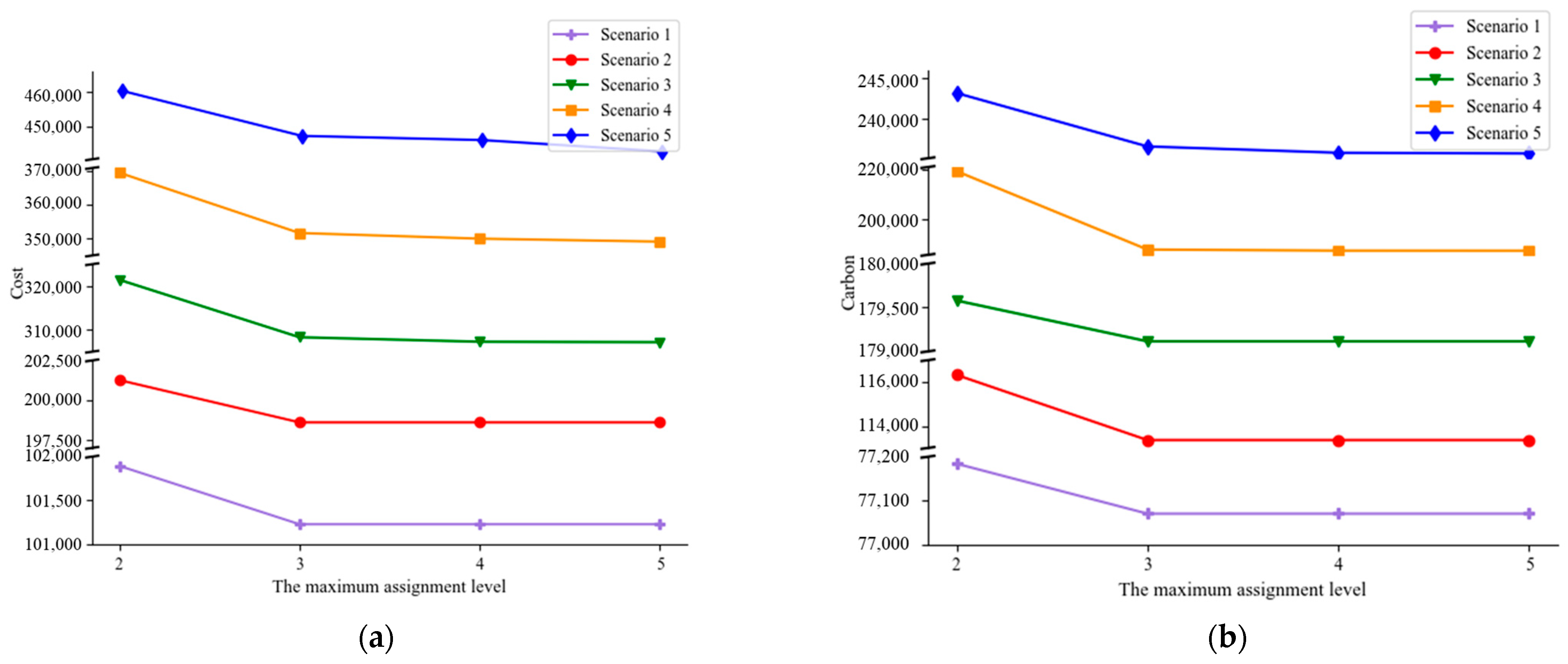
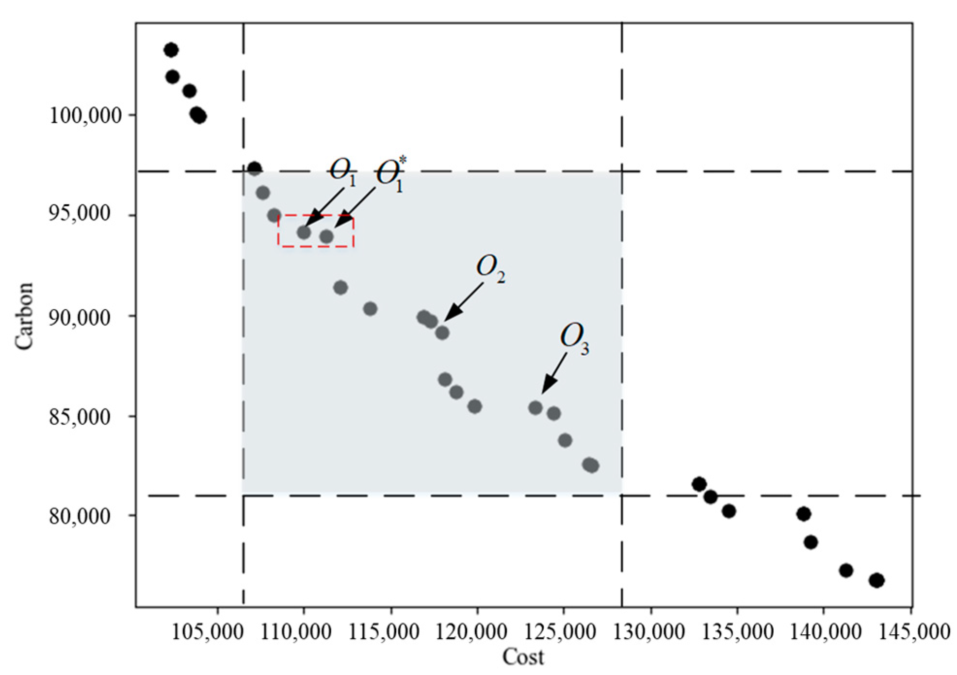
3.1. Problem Description

In this study, a three-echelon supply chain network comprising multiple suppliers, manufacturers, and customers was considered, as shown in Figure 1.

Manufacturers are owned by the enterprise, and they need various raw materials for production. The manager needs to select external candidate suppliers (the suppliers below are the candidate suppliers) to provide them with raw materials to produce products that will then be delivered to the customers. Owing to the influence of uncertain factors, suppliers have different degrees of disruption risks. To cope with the impact of disruptions, all raw materials that manufacturers require can be provided through a selection of suppliers at different levels; in the event of an outage by the supplier at the previous level, the supplier at the next level will provide their service. To ensure that customer demands are met even if all suppliers are disrupted, to prevent the entire supply chain from collapsing, this study built on the concepts of Zhang et al. [48] and Yan and Ji [14], who assumed that a temporary emergency supplier would be fully resilient to sudden disruptions due to its own measures (e.g., facility reinforcement); therefore, there was no risk of disruption.

In addition, the belief degree of the supplier’s disruption and fixed cost can vary depending on factors, such as geographic location and operating conditions. Furthermore, the unit cost and carbon emissions of each raw material that the manufacturer obtains from the supplier and the product that the customer obtains from the manufacturer also vary, depending on the chosen route and the production status of the enterprise. The consideration of cost and carbon emissions in this research includes all aspects of production, manufacturing, and transportation. For example, the unit cost or carbon emission of the product obtained by the customer from the manufacturer includes the cost or carbon emission of the product produced by the manufacturer and the transportation cost or carbon emission from the manufacturer to the customer. In addition, this study assumed that production is demand-driven (i.e., demand information is obtained through customers’ orders in advance).

Thus, to optimize the economic and low-carbon performance of the supply chain network, this model considered the two objectives of total cost and carbon emissions of the supply chain, and selected suppliers based on uncertainty disruptions. The level at which the selected suppliers provided raw materials to the manufacturers was determined, and the service manufacturers provided was optimized to meet customer demands.

3.2. Methodology

We considered a supply chain network composed of $S$ suppliers, $W$ manufacturers, and $I$ customers, where $s=1,2,\dots ,\left|S\right|$, $w=1,2,\dots ,\left|W\right|$, and $i=1,2,\dots ,\left|I\right|$, respectively. The fixed cost of supplier $s\in S$ is $r_s$, and the unit cost and carbon emission of obtaining each raw material $h\in H$ from supplier $s\in S$ by manufacturer $w\in W$ are $e_{swh}$ and $v_{swh}$, respectively. Each raw material required by each manufacturer was supplied by suppliers at most $L$ levels. For example, $L=3$ means that the possible supply levels $l$ are 1, 2, and 3. That is, the maximum possible supply level for a supply chain network with $L=3$ is 3; if a temporary emergency supplier is assigned before $l=3$, its supply level may also be 1 or 2. To quantify loss due to supplier disruption, a temporary emergency supplier with an index of 0 was introduced. This temporary emergency supplier was not a long-term partner, and certain measures, such as facility enhancement, can lead to extra expenses and generate carbon emissions; therefore, the unit cost and carbon emission of raw materials obtained by manufacturers from temporary emergency suppliers are typically much greater than materials obtained from long-term suppliers. The belief degree of the supplier’s uncertain disruption was provided based on expert estimation, denoted as $m_s\in (0,1),s=1,\dots ,\left|S\right|$, and the supplier’s disruptive events were independent. Hence, the uncertain disruption belief degree of supplier $s$ that supplies raw material $h$ to manufacturer $w$ can be denoted as $m_{swh}$. The belief degree of the temporary emergency supplier’s disruption was set as 0. For customer $i\in I$, whose demand is $q_i$, the unit cost and carbon emission for customer $i$ to obtain the product from manufacturer $w$ are $c_{wi}$ and $t_{wi}$, respectively.

Three categories of decision variables were associated with supply chain network optimization, that is, supplier selection variables $X_s$, assignment variables of suppliers to manufacturers $Z_{wslh}$, and manufacturers to customers $Y_{wi}$, where $Z_{wslh}$ means that for raw material $h$, supplier $s$ is assigned to manufacturer $w$ at level $l$. This represents the supplier to which the manufacturer is assigned when all the suppliers assigned at level $1,\dots ,l-1$ that provide raw material $h$ are disrupted. Unless the manufacturer is assigned to a temporary emergency supplier prior to the level $L$, each manufacturer will have exactly $L$ levels of assignment for each raw material. For raw material $h$, if a manufacturer is assigned to candidate suppliers at levels $1,\dots ,L-1$, then that manufacturer must be assigned to a temporary emergency supplier at level $L$, ensuring that the manufacturer’s needs are met in the event that all the suppliers assigned to the prior $L-1$ levels are disrupted.

Additionally, the uncertain variable $M_{wslh}$ was inducted to indicate the belief degree that for raw material $h$, suppliers assigned to manufacturer $w$ at levels $1,\cdots ,l-1$ are disrupted and the one assigned at level $l$ is normal. For this model, the indices, parameters, uncertain variables, and decision variables are shown below.

3.2.1. Notations

• Indices

$S$: set of suppliers, $s=1,2,\dots ,\left|S\right|$;

$W$: set of manufacturers, $w=1,2,\dots ,\left|W\right|$;

$I$: set of customers, $i=1,2,\dots ,\left|I\right|$;

$H$: set of raw materials, $h=1,2,\dots ,\left|H\right|$;

$L$: set of level, $l=1,2,\dots ,L$.

• Parameters

$q_i$: demand from customer $i$;

$r_s$: fixed cost of supplier $s$;

$e_{swh}$: unit cost of manufacturer $w$ obtaining raw material $h$ from supplier $s$;

$c_{wi}$: unit cost of customer $i$ obtaining the product from manufacturer $w$;

$m_{swh}$: uncertain disruption belief degree of supplier $s$ that supplies raw material $h$ to manufacturer $w$;

$v_{swh}$: unit carbon emission of manufacturer $w$ obtaining raw material $h$ from supplier $s$;

$t_{wi}$: unit carbon emission of customer $i$ obtaining the product from manufacturer $w$;

${\lambda }_{wh}$: quantity of raw material $h$ required by manufacturer $w$ to produce unit product;

$T{E}_{cap}$: supply chain total carbon emission cap;

$C{O}_{cap}$: supply chain total cost cap.

• Uncertain variables

$M_{wslh}$: for the raw material $h$, belief degree that suppliers assigned to manufacturer $w$ at levels $1,\dots ,l-1$ are disruptive and the one assigned at level $l$ is normal.

• Decision variables

$X_s=\{\begin{array}{l}1, \mathrm{if} \mathrm{supplier} s \mathrm{is} \mathrm{selscted},\\ 0, \mathrm{otherwise}.\end{array}$;

$Y_{wi}=\{\begin{array}{l}1, \mathrm{if} \mathrm{manufacturer} w \mathrm{is} \mathrm{assigned} \mathrm{to} \mathrm{customer} i,\\ 0, \mathrm{otherwise}.\end{array}$;

$Z_{wslh}=\{\begin{array}{l}1, \mathrm{for} \mathrm{the} \mathrm{raw} \mathrm{material} h,\mathrm{if} \mathrm{supplier} s \mathrm{is} \mathrm{assigned} \mathrm{to} \mathrm{manufacturer} w \mathrm{at} \mathrm{level} l,\\ 0, \mathrm{otherwise}.\end{array}$.

3.2.2. Model Formulation

The first objective of this study was to minimize the expected total cost of the supply chain network, $f_{\cos t}$:

$$\min f_{\cos t}={\displaystyle \sum _{s=1}^{\left|S\right|}{r}_s}{X}_s+{\displaystyle \sum _{i=1}^{\left|I\right|}{\displaystyle \sum _{h=1}^{\left|H\right|}{\displaystyle \sum _{s=0}^{\left|S\right|}{\displaystyle \sum _{w=1}^{\left|W\right|}{\displaystyle \sum _{l=1}^L{e}_{swh}{Z}_{wslh}{M}_{wslh}{\lambda }_{wh}}}}}{q}_i{Y}_{wi}}+{\displaystyle \sum _{i=1}^{\left|I\right|}{\displaystyle \sum _{w=1}^{\left|W\right|}{c}_{wi}}}{q}_i{Y}_{wi}$$

(1a)

where the first term deals with the fixed cost of selected suppliers; the expected cost of manufacturers obtaining various raw materials from the suppliers is indicated in the second term, and the cost of customers obtaining the products from the manufacturers is represented in the third term.

The second objective was to minimize the expected total carbon emissions of the supply chain network, $f_{carbon}$:

$$\min f_{carbon}={\displaystyle \sum _{i=1}^{\left|I\right|}{\displaystyle \sum _{h=1}^{\left|H\right|}{\displaystyle \sum _{s=0}^{\left|S\right|}{\displaystyle \sum _{w=1}^{\left|W\right|}{\displaystyle \sum _{l=1}^L{v}_{swh}{Z}_{wslh}{M}_{wslh}{\lambda }_{wh}{q}_i{Y}_{wi}}}}}}+{\displaystyle \sum _{i=1}^{\left|I\right|}{\displaystyle \sum _{w=1}^{\left|W\right|}{t}_{wi}}}{q}_i{Y}_{wi}$$

(1b)

where the first term represents the expected carbon emissions of manufacturers obtaining all raw materials from the suppliers, and the second term deals with the carbon emissions of customers obtaining the products from the manufacturers.

Constraint (1c) ensures that for each raw material, an unselected supplier cannot be assigned to the manufacturer:

$${\displaystyle \sum _{l=1}^L{Z}_{wslh}}\le X_s,\forall w\in W,s\in S,h\in H$$

(1c)

Constraint (1d) applies the restriction that, for each raw material, the manufacturer must have a candidate supplier for service at each level, unless a temporary emergency supplier is assigned at that level or before:

$${\displaystyle \sum _{s=1}^{\left|S\right|}{Z}_{wslh}}+{\displaystyle \sum _{p=1}^l{Z}_{w0ph}}=1,\forall w\in W,h\in H,l=1,\dots ,L$$

(1d)

Constraint (1e) specifies that, for each raw material, each manufacturer has to be assigned to a temporary emergency supplier at a certain level. Specifically, a temporary emergency supplier can ensure that all demands can be met when all assigned suppliers are disrupted:

$${\displaystyle \sum _{l=1}^L{Z}_{w0lh}}=1,\forall w\in W,h\in H$$

(1e)

To ensure that customer demands are met, constraint (1f) states that each customer must be assigned to a manufacturer:

$${\displaystyle \sum _{w=1}^{\left|W\right|}{Y}_{wi}}=1,\forall i\in I$$

(1f)

For each raw material, the belief degree that manufacturer $w$ is served normally when allocated to supplier $s$ at the first level can be calculated using constraint (1g):

$$M_{ws1h}=1-m_{wsh},\forall w\in W,s\in S,h\in H$$

(1g)

It is important to note that ${\displaystyle {\sum }_{k=1}^{\left|S\right|}{m}_{wkh}{Z}_{wkph}}={\displaystyle {\sum }_{k=0}^{\left|S\right|}{m}_{wkh}{Z}_{wkph}}$ is due to $m_{wkh}=0$ for $k=0$; thus, for raw material $h$, the disruption belief degree of the supplier to which manufacturer $w$ is assigned at level $p$ can be expressed as ${\displaystyle {\sum }_{k=1}^{\left|S\right|}{m}_{wkh}{Z}_{wkph}}$. The uncertainty theory has been considerably developed in terms of its theory and application since it was proposed; specific applications of the uncertainty theory can be found in the literature [49]. According to the uncertainty theory [15], and the literature on the application of the uncertainty theory [14], constraint (1h) calculates, for raw material $h$, the belief degree that manufacturer $w$ can be served normally when supplier $s$ is assigned to it for $l=2,\dots ,L$(i.e., supplier $s$ is normal, while suppliers assigned at prior levels are disrupted), in which $\wedge$ is an operator of the uncertainty theory and denotes the take-small operation:

$$M_{wslh}=\left(\underset{p=1}{\overset{l-1}{\wedge }}{\displaystyle \sum _{k=1}^{\left|S\right|}{m}_{wkh}{Z}_{wkph}}\right)\wedge (1-m_{wsh}),\forall w\in W,s\in S,l=2,\cdots ,L,h\in H$$

(1h)

Constraint (1i) guarantees that the decision variables are non-negative:

$$X_s,Y_{wi},Z_{wslh}\in \{0,1\},\forall s\in S,w\in W,i\in I,l=1,\cdots ,L,h\in H$$

(1i)

In conclusion, considering the two objectives of cost (1a) and carbon emissions (1b), and constraints (1c)−(1i), a multi-objective low-carbon supply chain network optimization model (LSM) with the risk of uncertain supply disruptions can be obtained.

4. Model Analysis

We further analyzed the model to facilitate its solution and strengthen the understanding of the management implications.

4.1. Supply Chain Uncertain Disruption Risk Analysis

The supply chain network disruption risk varies with the choice of different suppliers due to the varying degrees of the disruption risk of suppliers. To quantify this risk, the supply chain uncertain disruption risk (SCUDR) was defined in this research as the risk that all entities in the supply chain (including suppliers, manufacturers, and customers) will be affected by uncertain supply disruptions, which results in the supply chain being unable to provide services. According to the definition of SCUDR, quantified SCUDR is shown below:

Theorem. 

The risk of supply chain network with supply disruptions is:

$$SCUDR=\underset{h=1}{\overset{\left|H\right|}{\vee }}\underset{l=1}{\overset{L}{\wedge }}\left({\displaystyle \sum _{w=1}^{\left|W\right|}{\displaystyle \sum _{i=1}^{\left|I\right|}{\displaystyle \sum _{s=1}^{\left|S\right|}{m}_{wsh}{Z}_{wslh}}}}{\lambda }_{wh}{q}_i{Y}_{wi}\right)/{\displaystyle \sum _{w=1}^{\left|W\right|}{\displaystyle \sum _{h=1}^{\left|H\right|}{\displaystyle \sum _{i=1}^{\left|I\right|}{\lambda }_{wh}{q}_i{Y}_{wi}}}}$$

(1j)

Proof of Theorem.

Based on the uncertainty theory [15], since the belief degree of disruption $m_{wsh}$ in the supply chain is regarded as uncertain, from the supply side, ${\displaystyle {\sum }_{s=1}^{\left|S\right|}{m}_{wsh}{Z}_{wslh}}$ can represent the belief degree of disruption of the supplier providing raw material $h$ for manufacturer $w$ at level $l$ . From the manufacturing side, ${\displaystyle {\sum }_{s=1}^{\left|S\right|}{m}_{wsh}{Z}_{wslh}}$ can represent the belief degree of disruption of manufacturer $w$ for raw material $h$ at level $l$ . This is because if the supplier is disrupted, then the manufacturer will be unable to produce the finished product due to the lack of raw material $h$ , thus causing disruption. □

Since the production and delivery of the finished product requires that each raw material subsystem is working properly (i.e., without disruption), the supply chain can be regarded as a series system. Accordingly, the uncertain disruption risk of each subsystem is determined by minimizing the uncertain disruption risk of each manufacturer at each assignment level in this subsystem, then summing all manufacturers’ uncertain disruption risk, where the uncertain disruption risk at each level is determined using the belief degree of disruption and supply quantity. The larger the supply quantity, the greater the risk caused by disruption.

To understand this concept, we first began with a parallel system with one manufacturer and two suppliers, $s_1$ and $s_2$; the belief degree of disruption is denoted as $m_1$ and $m_2$, respectively, and $m_1<m_2$, with supply quantity $q$ and assignment levels $l_1$ and $l_2$. Further, if $m_{1}q$ is the uncertain disruption risk of $s_1$ operating at level $l_1$ and $m_{2}q$ is the uncertain disruption risk of $s_2$ operating at level $l_2$, then $SCUDR=m_{1}q$.

Thus, for a subsystem of $L$ levels, $\left|S\right|$ suppliers, $\left|W\right|$ manufacturers, and $\left|I\right|$ customers, based on the uncertainty theory [15], for raw material $h$, the uncertain disruption risk of manufacturer $w$ can be expressed as $\underset{l=1}{\overset{L}{\wedge }}{\displaystyle {\sum }_{s=1}^{\left|S\right|}{m}_{wsh}{Z}_{wslh}}{\displaystyle {\sum }_{i=1}^{\left|I\right|}{\lambda }_{wh}{q}_i{Y}_{wi}}$. Accordingly, for each raw material, the uncertain disruption risk can be calculated as: $SCUD{R}_h={\displaystyle {\sum }_{w=1}^{\left|W\right|}\underset{l=1}{\overset{L}{\wedge }}}\left({\displaystyle {\sum }_{s=1}^{\left|S\right|}{m}_{wsh}{Z}_{wslh}}\right){\displaystyle {\sum }_{i=1}^{\left|I\right|}{\lambda }_{wh}{q}_i{Y}_{wi}},\forall h\in H$. Therefore, the uncertain disruption risk for the entire supply chain network, that is, SCUDR, is calculated as: $SCUDR=\underset{h=1}{\overset{\left|H\right|}{\vee }}SCUD{R}_h/{\displaystyle {\sum }_{w=1}^{\left|W\right|}{\displaystyle {\sum }_{h=1}^{\left|H\right|}{\displaystyle {\sum }_{i=1}^{\left|I\right|}{\lambda }_{wh}{q}_i{Y}_{wi}}}}$, in which $\vee$ is an operator of the uncertainty theory and denotes the take-large operation. This leads to the following:

Property 1.

The SCUDR will be non-increasing with the increase in the maximum assignment level $L$.

Proof of Property 1.

According to the theorem above, when the maximum assignment level $L$ goes up, the belief degree of disruptions of manufacturer $w$ , i.e., $\underset{l=1}{\overset{L}{\wedge }}{\displaystyle {\sum }_{s=1}^{\left|S\right|}{m}_{wsh}{Z}_{wslh}}$, is non-increasing for raw material $h$. Therefore, as the maximum assignment level $L$ increases, the SCUDR is non-increasing. □

Property 1 indicates that, as the maximum assignment level $L$ increases, the manufacturer will be assigned to more suppliers, thus reducing the possibility of disruption. Therefore, the SCUDR will either stay the same or decrease. As different network structures correspond to different SCUDRs, decision makers can choose supply chain networks according to this index. Moreover, reasonably setting the maximum assignment level can significantly reduce the SCUDR, which provides theoretical guidance for designing supply chain networks that reduce risk and improve reliability.

4.2. Objective Function Analysis

To better support decision making, we analyzed the cost and carbon emission objectives, respectively, and obtained the following properties:

Property 2.

(i) The optimal objective value of the cost objective function $f_{\cos t}$ will be non-increasing as the maximum assignment level $L$ increases. (ii) The optimal objective value of the carbon emission objective function $f_{carbon}$ will be non-increasing as the maximum assignment level $L$ increases.

Proof of Property 2.

(i) If the decision maker has an ideal value for the carbon emission index in the model (LSM), it can be translated into a constraint. When the maximum assignment level equaled $\overline{L}$, the optimal solution was noted using $X_s^{*}$, $Y_{wi}^{*}$, $Z_{wslh}^{*}$, and $\forall s\in S,w\in W,i\in I,l=1,\cdots ,\overline{L},h\in H$, and the corresponding cost objective function value was represented as ${\varphi }^{*}$. A feasible solution can be constructed when $L=\overline{L}+1$. For all $\forall s\in S,w\in W,i\in I,l=1,\cdots ,\overline{L},h\in H$, we let $X_s^{’}=X_s^{*},Y_{wi}^{’}=Y_{wi}^{*}$ and $Z_{wslh}^{’}=Z_{wslh}^{*}$. For $l=\overline{L}+1$, we let $Z_{wslh}^{’}=0$. When the maximum assignment level was $\overline{L}+1$, $X_s^{*},Y_{wi}^{*}$ and $Z_{wslh}^{*}$ were able to satisfy constraints (1c)−(1i) and the carbon emission constraint. The objective value remains unchanged; thus, its optimal objective value was less than or equal to ${\varphi }^{*}$. Similarly, when the decision maker has an ideal value for the cost objective, it can also be translated into a constraint. The above proof can thereby be used to prove property 2(ii). □

Property 2 shows that, as $L$ increases, there will be more feasible network structures to select; thus, the optimal objective value will at least not increase. Nevertheless, when $L$ is set too high, manufacturers are likely to be allocated to distant suppliers at some levels on account of the high unit cost (carbon emissions) of supplying directly from the temporary emergency supplier. Therefore, it will be difficult to meet manufacturers’ needs in a timely manner when many suppliers are disrupted, which leads to a reduced willingness in manufacturers and suppliers to work together in the long term. Furthermore, a high $L$ will cause excessive decision variables and constraints, which complicates the solution procedure. As a result, while $L$ can be at most equivalent to $\left|S\right|+1$, the decision maker must set this parameter according to the actual requirements.

Property 3.

(i) The optimal objective value of the cost objective function $f_{\cos t}$ will be non-increasing as the carbon emission constraint $T{E}_{cap}$ increases. (ii) The optimal objective value of the carbon emission objective function $f_{carbon}$ will be non-increasing as the cost constraint $C{O}_{cap}$ increases.

Proof of Property 3.

(i) If the decision maker has an ideal value for the carbon emission index in the model (LSM), it can be translated into a constraint. The optimal solution is denoted by $X_s^{*},Y_{wi}^{*}$, $Z_{wslh}^{*}$, and $\forall s\in S,w\in W,i\in I,l=1,\cdots ,L,h\in H$, and the corresponding cost objective function value is marked as ${\varphi }^{*}$ if the carbon emission constraint is equivalent to ${\overline{TE}}_{cap}$. Evidently, when the carbon emission constraint is greater than ${\overline{TE}}_{cap}$, $X_s^{*},Y_{wi}^{*}$ and $Z_{wslh}^{*}$ can satisfy constraints (1c)−(1i) and the carbon emission constraint. The objective value remains unchanged; thus, its optimal objective value was less than or equal to ${\varphi }^{*}$. Similarly, when the decision maker has an ideal value for the cost objective, it can also be translated into a constraint. The above proof can thereby be used to prove property 3(ii). □

Property 3 suggests that as the carbon emission constraint $T{E}_{cap}$ or cost constraint $C{O}_{cap}$ decreases, the feasible region will expand and there will be more viable network structures to choose from; thus, the optimal objective value will at least not increase.

4.3. Linearized Constraint

In this model (LSM), constraint (1h) is nonlinear, which can be converted into a linear form via the introduction of an auxiliary 0–1 decision variable, $u_p^{wslh}$, to facilitate the solution. For each $s\in S,w\in W,i\in I,l=2,\dots ,L,h\in H$, constraint (1h) can be replaced with a new set of constraints as follows:

$$M_{wslh}\le 1-m_{wsh}$$

$$M_{wslh}\le {\displaystyle \sum _{k=1}^{\left|S\right|}{m}_{wkh}}{Z}_{wkph},\forall p=1,\dots ,l-1$$

$$M_{wslh}+B(1-u_l^{wslh})\ge 1-m_{wsh}$$

$$M_{wslh}+B(1-u_p^{wslh})\ge {\displaystyle \sum _{k=1}^{\left|S\right|}{m}_{wkh}}{Z}_{wkph},\forall p=1,\dots ,l-1$$

$${\displaystyle \sum _{p=1}^l{u}_p^{wslh}}=1$$

$$u_p^{wslh}\in \{0,1\},\forall p=1,\dots ,l$$

We can denote this set of constraints as (MT), where $B$ denotes a large number. The first two constraints guarantee that $M_{wslh}$ is not greater than $\left(\underset{p=1}{\overset{l-1}{\wedge }}{\displaystyle {\sum }_{k=1}^{\left|S\right|}{m}_{wkh}{Z}_{wkph}}\right)\wedge (1-m_{wsh})$. The last four constraints enforce that $M_{wslh}$ is greater than or equal to one value in $\left\{1-m_{wsh},{\displaystyle {\sum }_{k=1}^{\left|S\right|}{m}_{wkh}{Z}_{wk1h}},\dots ,{\displaystyle {\sum }_{k=1}^{\left|S\right|}{m}_{wkh}{Z}_{wklh}}\right\}$, which is equivalent to at least their minimum. Therefore, constraint (MT) is equivalent to constraint (1h).

5. Solution Method

This study considered the different needs of decision makers and used various methods to solve the model according to different decision criteria, including bi-objective transformation into single-objective optimization, and bi-objective optimization to provide the Pareto solution set.

5.1. Considering Single-Objective Optimization

5.1.1. Minimizing Cost

When a decision maker has an ideal value for the carbon emission objective, it can be transformed into a carbon emission constraint (i.e., a single-objective model with the objective of minimizing cost, denoted SLSM) as follows:

$$\min {\displaystyle \sum _{s=1}^{\left|S\right|}{r}_s}{X}_s+{\displaystyle \sum _{i=1}^{\left|I\right|}{\displaystyle \sum _{h=1}^{\left|H\right|}{\displaystyle \sum _{s=0}^{\left|S\right|}{\displaystyle \sum _{w=1}^{\left|W\right|}{\displaystyle \sum _{l=1}^L{e}_{swh}{Z}_{wslh}{M}_{wslh}{\lambda }_{wh}}}}}{q}_i{Y}_{wi}}+{\displaystyle \sum _{i=1}^{\left|I\right|}{\displaystyle \sum _{w=1}^{\left|W\right|}{c}_{wi}}}{q}_i{Y}_{wi}$$

(2a)

The constraints contain (1c)–(1g), (1i), (MT), and (2b), where (2b) is shown be-low:

$${\displaystyle \sum _{i=1}^{\left|I\right|}{\displaystyle \sum _{h=1}^{\left|H\right|}{\displaystyle \sum _{s=0}^{\left|S\right|}{\displaystyle \sum _{w=1}^{\left|W\right|}{\displaystyle \sum _{l=1}^L{v}_{swh}{Z}_{wslh}{M}_{wslh}{\lambda }_{wh}{q}_i{Y}_{wi}}}}}}+{\displaystyle \sum _{i=1}^{\left|I\right|}{\displaystyle \sum _{w=1}^{\left|W\right|}{t}_{wi}}}{q}_i{Y}_{wi}\le T{E}_{cap}$$

(2b)

5.1.2. Minimizing Carbon Emission

When a decision maker has an ideal value for the cost objective, it can be transformed into a cost constraint (i.e., a single-objective model with the objective of minimizing carbon emissions, denoted CSLSM) as follows:

$$\min {\displaystyle \sum _{i=1}^{\left|I\right|}{\displaystyle \sum _{h=1}^{\left|H\right|}{\displaystyle \sum _{s=0}^{\left|S\right|}{\displaystyle \sum _{w=1}^{\left|W\right|}{\displaystyle \sum _{l=1}^L{v}_{swh}{Z}_{wslh}{M}_{wslh}{\lambda }_{wh}{q}_i{Y}_{wi}}}}}}+{\displaystyle \sum _{i=1}^{\left|I\right|}{\displaystyle \sum _{w=1}^{\left|W\right|}{t}_{wi}}}{q}_i{Y}_{wi}$$

(3a)

The constraints contain (1c)–(1g), (1i), (MT), and (3b), where (3b) is shown below:

$${\displaystyle \sum _{s=1}^{\left|S\right|}{r}_s}{X}_s+{\displaystyle \sum _{i=1}^{\left|I\right|}{\displaystyle \sum _{h=1}^{\left|H\right|}{\displaystyle \sum _{s=0}^{\left|S\right|}{\displaystyle \sum _{w=1}^{\left|W\right|}{\displaystyle \sum _{l=1}^L{e}_{swh}{Z}_{wslh}{M}_{wslh}{\lambda }_{wh}}}}}{q}_i{Y}_{wi}}+{\displaystyle \sum _{i=1}^{\left|I\right|}{\displaystyle \sum _{w=1}^{\left|W\right|}{c}_{wi}}}{q}_i{Y}_{wi}\le C{O}_{cap}$$

(3b)

These models (SLSM and CSLSM) were solved directly using Gurobi 9.1.2.

5.2. Bi-Objective Optimization

If a decision maker pursues both the cost and carbon emission objectives, but these two objectives conflict with each other and no solution is available to optimize both objectives simultaneously, a satisfactory solution set can be provided for the decision makers to weigh the two objective functions. We designed a fast non-dominated sorting NSGA-II algorithm with an elite strategy, based on Deb et al. [50], to provide the satisfactory solution set for bi-objective optimization. The model (LSM) was solved using the proposed NSGA-II algorithm. Figure 2 shows the specific algorithm flowchart, and each step is described in detail below:

Step 1: Initialize the population and configure the evolutionary algebra $Gen=1$. To satisfy constraints (1c)−(1i), suppliers are first randomly selected. Then, based on the selection of suppliers, suppliers that can provide services are randomly assigned to each manufacturer level by level, and manufacturers are randomly assigned to each customer. After obtaining the randomly generated chromosome, if a manufacturer is not assigned to a temporary emergency supplier at any level, its assignment at the last level is modified to a temporary emergency supplier to ensure that the demands have been met.

Step 2: Identify whether the first-generation progeny population has been created. If so, let the evolutionary algebra $Gen=2$; otherwise, perform non-dominated sorting, tournament selection, simulated binary crossover, and polynomial variation to produce the first-generation progeny population and let $Gen=2$. It should be noted that constraint (1c) needs to be dealt with after the variation operation is performed as the selection of suppliers has changed. If a manufacturer is assigned to a supplier that has not been selected, it will be reassigned to a supplier that has been selected but does not provide services to it.

Step 3: Create a new population by merging the parent and offspring populations.

Step 4: Identify whether a new parent population has been created. If not, compute the objective functions, $f_{\cos t}$ and $f_{carbon}$, of the individuals in the new population, perform fast non-dominated sorting, compute the crowded distance, and implement the elite strategy to produce a new parent population. Otherwise, execute Step 5.

Step 5: Tournament selection, simulated binary crossover, and polynomial variation are performed on the generated parent population to generate the offspring population.

Step 6: Identify whether the evolutionary algebra $Gen$ is equivalent to the largest evolutionary algebra. If not, let $Gen=Gen+1$ and go back to Step 3. Else, the run ends.

6. Case Study

6.1. Case Description

This study examined the supply chain network design of a glass manufacturing company in China, which is engaged in the production of glass bottles for canning a variety of products, such as juice, syrup, milk, and jam. On the one hand, due to pressure from environmental laws and regulations, and customers, this company has made carbon emissions a goal in designing its supply chain network. On the other hand, this company’s supply chain network has experienced some major disruptions in the past few years, such as snow disasters, supplier fires, and the COVID-19 outbreak, resulting in significant cost losses. To address this company’s predicament, we applied our model to redesign the company’s supply chain network.

We considered the network construction under five scenarios in this case, each corresponding to the company’s different strategic plans, to demonstrate the validity of the presented model and to verify its applicability under different scenarios. In these scenarios, the number of candidate suppliers was 8, 10, 15, 20, and 25; the number of manufacturers was 9, 15, 30, 30, and 40; and the number of customers was 10, 20, 40, 70, and 96, respectively, all of whom are from medium- and large-sized cities in China. The possible maximum assignment levels were 2, 3, 4, and 5. The data related to the supply chain network operations, including the fixed cost of supplier openness, customer demands, and the costs and carbon emissions associated with obtaining raw materials and product, were provided by the company. However, there were no sufficient historical data or specialized records for the belief degree of the supplier’s disruption; thus it was given based on expert empirical estimation, and the belief degree of the supplier’s uncertain disruption given empirically did not exceed 0.2. All case studies were implemented on a laptop with an Intel i7-10510U CPU and 16 GB RAM. The optimal supply chain network structure of $L=3$ under Scenario 1 has been depicted in Figure 3.

6.2. Analysis of the Single-Objective Optimization Results

6.2.1. Analysis of the Cost and Carbon Emission Objectives

Table 2. Cost objective model solution results.

Scenario	$\left|\mathit{S}\right|$	$\left|\mathit{W}\right|$	$\left|\mathit{I}\right|$	$\mathit{L}=2$		$\mathit{L}=3$		$\mathit{L}=4$		$\mathit{L}=5$
				Cost	Time (s)	Cost	Time (s)	Cost	Time (s)	Cost	Time (s)
1	8	9	10	101,894.29	3	101,227.11	7	101,227.07	260	101,227.07	1365
2	10	15	20	201,264.04	70	198,604.97	177	198,604.95	645	198,604.94	3550
3	15	30	40	321,446.67	880	308,306.26	1902	307,274.19	6577	307,174.21	23,802
4	20	30	70	369,613.26	2040	351,676.67	3912	349,999.96	9112	349,117.64	45,507
5	25	40	96	460,326.06	6890	447,414.39	13,020	446,221.27	36,515	442,973.05	66,400

and

Table 3. Carbon emission objective model solution results.

Scenario	$\left|\mathit{S}\right|$	$\left|\mathit{W}\right|$	$\left|\mathit{I}\right|$	$\mathit{L}=2$		$\mathit{L}=3$		$\mathit{L}=4$		$\mathit{L}=5$
				Carbon	Time (s)	Carbon	Time (s)	Carbon	Time (s)	Carbon	Time (s)
1	8	9	10	77,184.19	6	77,070.32	15	77,070.31	568	77,070.31	3001
2	10	15	20	116,328.13	113	113,360.75	311	113,360.74	820	113,360.74	4707
3	15	30	40	179,579.50	1340	179,114.87	2443	179,114.87	8560	179,114.86	30,910
4	20	30	70	219,364.84	3504	188,111.38	5890	187,678.54	16,670	187,655.44	56,354
5	25	40	96	243,227.84	7988	236,655.62	17,038	235,879.59	48,633	235,791.75	85,905

show the solution results of the SLSM and CSLSM models, respectively, from which Figure 4 was derived. Figure 4a,b present the trend of the total cost and carbon emissions with the maximum assignment level $L$, respectively, in which “Time” is the running time of the algorithm.

Table 2 and Table 3 and Figure 4 demonstrate that the cost and carbon emission objective values are non-increasing as $L$ increases under the same scenario, which is consistent with Property 2. In addition, changes in the cost and carbon emission objective values were the most obvious as $L$ changed from two to three, following which the downtrend was not obvious, which provides the basis for reasonably setting this parameter.

In the following section, the SLSM model has been analyzed as an example. Considering the current economic capacity limit (below 150,000) and the carbon emission constraint limit (below 90,000) of the company, it has been further analyzed under Scenario 1, where $L=2,3,4$ has been chosen, as it has little effect on the objective value when $L$ is too large. According to the subsequent development of this company, managers can select other scales of the supply chain network’s structure to be similarly analyzed.

6.2.2. Analysis of the Multi-Level Backup Strategy for Uncertain Disruptions

To validate the proposed supply chain network optimization model in handling the risk of uncertain disruptions, the proposed optimal supply chain network optimization model was compared with the optimal network optimization model of the deterministic model under normal conditions [51].

Table 4. Comparison of the results between the proposed model and the deterministic model.

	$\mathbf{C}{\mathbf{O}}_{\mathit{N}}$	${\mathbf{\Delta }}_{\mathit{N}}$	$\mathit{\%}{\mathbf{\Delta }}_{\mathit{N}}$	$\mathbf{C}{\mathbf{O}}_{\mathit{D}}$	${\mathbf{\Delta }}_{\mathit{D}}$	$\mathit{\%}{\mathbf{\Delta }}_{\mathit{D}}$
Deterministic	91,321.84	-	-	131,677.42	-	-
$L=2$	96,729.11	5407.27	5.92	101,894.29	−29,783.13	−22.62
$L=3$	94,717.96	3396.12	3.71	101,227.11	−30,450.31	−23.12
$L=4$	94,717.96	3396.12	3.71	101,227.07	−30,450.33	−23.12

concludes the comparative results of the two models, in which $C{O}_N$ and $C{O}_D$ represent the cost under normal conditions and uncertain disruptions respectively. The cost increase (rate) of the proposed model versus the deterministic model under normal conditions has been denoted as ${\Delta }_N$($\%{\Delta }_N$), and ${\Delta }_D$($\%{\Delta }_D$) represents the cost increase (rate) under an uncertain disruption risk.

Table 4 indicates that compared with the deterministic model, taking uncertain disruptions into account at the design stage can significantly reduce costs, and it does not add much to the cost under normal conditions. In particular, using the results for $L=4$, the cost can be reduced by 23.12% when there is a risk of uncertain disruptions, compared with the normal increase of 3.71%. Thus, even if only the supply chain network results formed by $L=2$ are used to resolve the risk of uncertain disruptions, the expected cost can be reduced by 22.62%, while the cost increased by 5.92% under normal conditions.

Next, sensitivity analysis was conducted for specific parameters, such as the carbon emission cap and the belief degree of disruption, to provide a decision-making reference for the low-carbon supply chain network design under an uncertain environment.

6.2.3. Analysis of the Impact of the Carbon Emission Constraint

To validate the feasibility of the proposed supply chain network optimization model when addressing a higher carbon emission constraint, the effect of the carbon emission constraint on the cost under different $L$ is shown in

Table 5. Comparison of the cost objectives under different carbon emission constraints.

Carbon Emission Constraint	$\mathbf{L}=2$		$\mathbf{L}=3$		$\mathbf{L}=4$
	Cost	${\mathit{n}}_{\mathit{s}}$	Cost	${\mathit{n}}_{\mathit{s}}$	Cost	${\mathit{n}}_{\mathit{s}}$
800,000	101,894.29	3	101,227.11	4	101,227.07	4
80,000	105,174.69	3	102,010.52	5	102,010.52	5
79,000	107,497.87	3	103,875.49	4	103,875.49	4
78,000	110,920.43	3	106,239.15	4	106,239.15	4

, where $n_s$ denotes the number of selected suppliers.

As shown in Table 5, for the same $L$, the cost is non-decreasing with the increase in the carbon emission constraint, which is in line with Property 3, and the number of selected suppliers will at least not decrease as the carbon emission constraint is enhanced compared to the low carbon emission constraint (i.e., $T{E}_{cap}=800,000$). This is because when such uncertain disruptions exist, if the number of selected suppliers is reduced, the likelihood of manufacturers being assigned to the temporary emergency supplier increases, which will lead to a high carbon emission constraint that cannot be met. In addition, a more stringent carbon emission constraint can be met without increasing the cost by reasonably setting $L$ to account for uncertain disruptions. For example, the cost (106,239.15) with $L=3$ at a carbon emission constraint of 78,000 is lower than that (107,497.87) with $L=2$ at a carbon emission constraint of 79,000. Therefore, a supply chain network with a multi-level backup strategy should be implemented to facilitate the decarbonization of the supply chain in the face of the shock of uncertain disruption risks.

6.2.4. Analysis of the Impact of the Belief Degree of Disruption

To explore the effect of the belief degree of uncertain supply disruptions on the supply chain network, results of a high carbon emission constraint (i.e.,$T{E}_{cap}=79,000$) was compared with different belief degrees (

Table 6. Comparison of the cost objectives under different belief degrees.

Belief Degree of Disruption	$\mathbf{L}=2$		$\mathbf{L}=3$		$\mathbf{L}=4$
	Cost	${\mathit{n}}_{\mathit{s}}$	Cost	${\mathit{n}}_{\mathit{s}}$	Cost	${\mathit{n}}_{\mathit{s}}$
0	91,321.84	3	91,321.84	3	91,321.84	3
$0.5m_s$	96,970.44	3	96,386.97	4	96,386.97	4
$m_s$	107,497.87	3	103,875.49	4	103,875.49	4
$1.5m_s$	114,928.44	3	109,422.94	5	109,422.94	5
$2m_s$	133,909.63	3	125,281.82	4	125,281.82	4

), where $n_s$ denotes the number of selected suppliers. From Table 6, Figure 5a can be derived, which presents the changes in the cost objective value with $L$ under different belief degrees, and Figure 5b, which displays the changes in the cost objective values with belief degrees under different $L$.

As shown in Table 6 and Figure 5, for the same $L$, mitigating the risk of uncertain disruptions always requires a higher cost with the increase in the belief degree. This is because, as more disruptions create difficulties in meeting demand, the temporary emergency supplier has to provide services, thus increasing costs. Furthermore, the number of selected suppliers will at least not decrease as the belief degree of disruption increases compared to without disruption. This is because increasing the number of suppliers provides manufacturers with more viable options, while also avoiding the high cost of using a temporary emergency supplier.

In addition, with a high carbon emission constraint, the effect of a multi-level backup becomes more significant as the belief degree of supply disruption increases. For example, when $L$ changes from two to three, the cost is reduced by 3622.38 with a normal belief degree of disruption, and that is reduced by 5505.5 with 1.5 times the belief degree of disruption. This is because the likelihood of activating the “backup chain” increases as the belief degree of disruption increases. Therefore, the greater the belief degree of supply disruption, the more necessary it is to adopt a multi-level backup strategy to optimize the supply chain network’s structure.

6.2.5. Analysis of the Supply Chain Uncertain Disruption Risk

Table 7. Relationship between the SCUDR and the cost objective.

Carbon Emission Constraint	$\mathbf{L}=2$			$\mathbf{L}=3$			$\mathbf{L}=4$
	Cost	SCUDR	Carbon	Cost	SCUDR	Carbon	Cost	SCUDR	Carbon
82,000	101,974.19	0.0801	81,856.34	101,227.11	0.0496	80,778.21	101,227.11	0.0496	80,778.21
81,000	102,531.16	0.0722	80,971.88	101,227.11	0.0496	80,778.21	101,227.11	0.0496	80,778.21
80,000	105,174.69	0.0866	79,876.42	102,010.52	0.0629	79,081.33	102,010.52	0.0629	79,081.33
79,000	107,497.87	0.0866	78,777.02	103,875.49	0.0496	78,324.15	103,875.49	0.0496	78,324.15
78,000	110,920.43	0.0803	77,794.37	106,239.15	0.0408	77,241.78	106,239.15	0.0408	77,241.78

shows the relationship between the cost objective and the SCUDR, and the SCUDR under different $L$. Accordingly, Figure 6 can be derived, which shows the changes in the SCUDR with $L$ under different carbon emission constraints, and the changes in the SCUDR with cost under different $L$.

As shown in Table 7 and Figure 6, for the same $L$, the SCUDR increases and then decreases as the cost increases. This is because, to minimize the cost objective while meeting a higher carbon emission constraint, manufacturers may be assigned to suppliers with lower carbon emissions but higher disruption risk; thus, the SCUDR presents a non-decreasing scenario. However, when the cost is very high, that is, when the carbon emission constraint is very high (i.e.,$T{E}_{cap}<80,000$), the enterprise will choose to sacrifice part of its own benefits by selecting the risker path to meet the carbon emission constraint.

In addition, the SCUDR is non-increasing as $L$ increases under the same carbon emission constraint, which is in accordance with Property 1. Therefore, to design a low-risk, high-reliability supply chain network under such an uncertain disruption, the supply chain should be effectively coordinated to determine the maximum assignment level. If the carbon emission constraint is large enough, for example, when the carbon emission constraint is greater than or equal to 81,000 and $L=3$, the reliability of the supply chain network with the same network structure remains the same. At this point, the supply chain can participate in carbon trading and sell their excess carbon quota to increase their revenue.

6.3. Analysis of the Bi-Objective Optimization Results

The analysis of the solution of the model (LSM) is described in this section. For the bi-objective problem, $L=2$ in Scenario 1 is presented as an example. In this scenario, the population size was 100; maximum number of generations was 100; probability of crossover was 0.8; and the probability of mutation was 0.05.

As Figure 7 shows, a significant negative correlation exists between the cost and carbon emissions, and they cannot be concurrently minimized. Therefore, it is unlikely to achieve the optimal solution to simultaneously meet the objectives of minimizing the cost and carbon emissions. This implies that the cost will increase as the carbon emissions decrease, and vice versa. Therefore, decision makers must weigh lowering the total cost against reducing the carbon emissions when finalizing their choices.

Generally, decision makers will pay more attention to a certain range of solution sets on the Pareto front. For example, the solution set of the shaded part in Figure 7 is the range to which decision makers will give greater focus. Based on the solution on the Pareto front, the SCUDR of the corresponding supply chain network’s structure is obtained. For example, in Figure 7, the cost, carbon emissions, and SCUDR of $O_1$ are 109,305.77, 94,107.23, and 0.0838; $O_1^{*}$ are 111,317.36, 93,909.54, and 0.0836; $O_2$ are 117,502.61, 89,136.52, and 0.0776; and $O_3$ are 123,805.87, 85,090.26, and 0.0739, respectively. Decision makers can use the above relevant indicators to choose the right solution for them. In addition, by observing the points $O_1$ and $O_1^{*}$ in the red dotted box, it can be seen that $O_1$ has a significant reduction in its cost (by 2011.59), with no significant changes in its carbon emissions (only 197.69 higher); however, the SCUDR increased slightly (by 0.0002). Accordingly, a decision maker who is less risk-sensitive should choose $O_1$. Therefore, decision makers should place more focus on key schemes in which there is no significant change in one indicator but significant changes in others.

7. Conclusions

This study explored the low-carbon supply chain network’s design in the presence of an uncertain supply disruption risk. A bi-objective uncertain nonlinear mixed-integer programming model was developed by considering the objectives of minimizing the carbon emissions and costs. The model first selects suppliers with uncertain disruptions, then completes the assignment of suppliers and manufacturers to satisfy customer needs. Furthermore, we defined and quantified the SCUDR; the properties of the proposed model were discussed. Then, the nonlinear constraint in the model was linearized using the proposed techniques. The model was solved using various methods according to different decision criteria. The proposed supply chain network optimization model can not only provide optimal solutions when the probability distribution of disruptions is unknown but can also serve as a decision framework for the low-carbon supply chain network’s design in an uncertain environment.

These results indicate that compared with the deterministic model, taking uncertain disruptions into account at the design stage can significantly reduce costs when disruptions occur, and it does not add much to the cost under normal conditions. Second, by properly setting the maximum assignment level to manage the risk of uncertain disruptions, more stringent carbon emission requirements can be met and the SCUDR can be reduced without increasing the cost. Third, with a high carbon emission constraint, the effect of a multi-level backup becomes more significant as the belief degree of supply disruption increases. Fourth, a significant negative correlation exists between the cost and carbon emissions, and they cannot be concurrently minimized. Therefore, facing the increasing uncertainty of the external environment, it is necessary for decision makers to adopt the multi-level backup strategy to optimize the supply chain network’s structure. This will help decision makers in designing a reliable supply chain network under an uncertain environment that can operate well at a lower cost and with fewer carbon emissions, regardless of whether supply disruptions occur.

Some limitations exist in the present study, which suggest directions for future research. First, the facility capacity and disruptions of other entities were not considered, which should be considered in future research to make the model more complete. Second, only single-periodicity scenarios were considered in this study; in the future, a multi-periodicity supply chain network design can be conducted in conjunction with the actual needs. Finally, the SCUDR is also an issue of concern for decision makers. Therefore, the SCUDR, as defined in this study, could be incorporated into the model as an objective; then, the trade-off between cost, carbon emissions, and SCUDR could be analyzed.

References

1. Peura, H.; Bunn, D.W. Renewable power and electricity prices: The impact of forward markets. Manag. Sci. 2021, 67, 4772–4788. [Google Scholar] [CrossRef]
2. Frank, A.G.; Dalenogare, L.S.; Ayala, N.F. Industry 4.0 technologies: Implementation patterns in manufacturing companies. Int. J. Prod. Econ. 2019, 210, 15–26. [Google Scholar] [CrossRef]
3. Han, B.; Zhang, Y.; Wang, S.; Park, Y. The efficient and stable planning for interrupted supply chain with dual-sourcing strategy: A robust optimization approach considering decision maker’s risk attitude. Omega 2023, 115, 102775. [Google Scholar] [CrossRef]
4. Li, G.; Wu, H.; Sethi, S.P.; Zhang, X. Contracting green product supply chains considering marketing efforts in the circular economy era. Int. J. Prod. Econ. 2021, 234, 108041. [Google Scholar] [CrossRef]
5. Snoeck, A.; Udenio, M.; Fransoo, J.C. A stochastic program to evaluate disruption mitigation investments in the supply chain. Eur. J. Oper. Res. 2019, 274, 516–530. [Google Scholar] [CrossRef]
6. Kinra, A.; Ivanov, D.; Das, A.; Dolgui, A. Ripple effect quantification by supplier risk exposure assessment. Int. J. Prod. Res. 2020, 58, 5559–5578. [Google Scholar] [CrossRef]
7. Amiriaref, M.; Klibi, W.; Babai, M.Z. The multi-sourcing location inventory problem with stochastic demand. Eur. J. Oper. Res. 2018, 266, 72–87. [Google Scholar] [CrossRef]
8. Hall, P.V. “We’d have to sink the ships”: Impact studies and the 2002 West Coast port lockout. Econ. Dev. Q. 2004, 18, 354–367. [Google Scholar] [CrossRef]
9. Ivanov, D.; Tang, C.S.; Dolgui, A.; Battini, D.; Das, A. Researchers’ perspectives on Industry 4.0: Multi-disciplinary analysis and opportunities for operations management. Int. J. Prod. Res. 2021, 59, 2055–2078. [Google Scholar] [CrossRef]
10. Banks, E. Catastrophic Risk: Analysis and Management; John Wiley & Sons: New York, NY, USA, 2005. [Google Scholar]
11. Taleb, N.N. The Black Swan: The Impact of the Highly Improbable; Random House: New York, NY, USA, 2007. [Google Scholar]
12. Saghafian, S.; Van Oyen, M.P. The value of flexible backup suppliers and disruption risk information: Newsvendor analysis with recourse. IIE Trans. 2012, 44, 834–867. [Google Scholar] [CrossRef]
13. Lim, M.K.; Bassamboo, A.; Chopra, S.; Daskin, M.S. Facility location decisions with random disruptions and imperfect estimation. Manuf. Serv. Oper. Manag. 2013, 15, 239–249. [Google Scholar] [CrossRef]
14. Yan, S.; Ji, X. Supply chain network design under the risk of uncertain disruptions. Int. J. Prod. Res. 2020, 58, 1724–1740. [Google Scholar] [CrossRef]
15. Liu, B. Uncertainty Theory: A Branch of Mathematics for Modeling Human Uncertainty; Springer: Berlin, Germany, 2010. [Google Scholar]
16. Kazançoglu, Y.; Ozturkoglu, Y.; Mangla, S.K.; Ozbiltekin-Pala, M.; Ishizaka, A. A proposed framework for multi-tier supplier performance in sustainable supply chains. Int. J. Prod. Res. 2022, 23, 531–555. [Google Scholar] [CrossRef]
17. Hammami, R.; Nouira, I.; Frein, Y. Carbon emissions in a multi-echelon production-inventory model with lead time constraints. Int. J. Prod. Econ. 2015, 164, 292–307. [Google Scholar] [CrossRef]
18. Mohammed, F.; Selim, S.Z.; Hassan, A.; Syed, M.N. Multi-period planning of closed-loop supply chain with carbon policies under uncertainty. Transport. Res. Part D-Transport. Environ. 2017, 51, 146–172. [Google Scholar] [CrossRef]
19. Zhou, Y.; Gong, D.C.; Huang, B.; Peters, B.A. The impacts of carbon tariff on green supply chain design. IEEE Trans. Autom. Sci. Eng. 2017, 14, 1542–1555. [Google Scholar] [CrossRef]
20. Marufuzzaman, M.; Ekşioğlu, S.D.; Hernandez, R. Environmentally friendly supply chain planning and design for biodiesel production via wastewater sludge. Transp. Sci. 2014, 48, 555–574. [Google Scholar] [CrossRef]
21. Hong, Z.; Dai, W.; Luh, H.; Yang, C. Optimal configuration of a green product supply chain with guaranteed service time and emission constraints. Eur. J. Oper. Res. 2018, 266, 663–677. [Google Scholar] [CrossRef]
22. Kumari, M.; De, P.K.; Narang, P.; Shah, N.H. Integrated optimization of inventory, replenishment, and vehicle routing for a sustainable supply chain utilizing a novel hybrid algorithm with carbon emission regulation. Expert Syst. Appl. 2023, 220, 119667. [Google Scholar] [CrossRef]
23. Garcia-Castro, F.L.; Ruiz-Femenia, R.; Salcedo-Diaz, R.; Caballero, J.A. Sustainable supply chain design under correlated uncertainty in energy and carbon prices. J. Clean Prod. 2023, 414, 137612. [Google Scholar] [CrossRef]
24. Abbasi, S.; Erdebilli, B. Green closed-loop supply chain networks’ response to various carbon policies during COVID-19. Sustainability 2023, 15, 3677. [Google Scholar] [CrossRef]
25. Kabiri, N.N.; Emami, S.; Safaei, A.S. Simulation–optimization approach for the multi-objective production and distribution planning problem in the supply chain: Using NSGA-II and Monte Carlo simulation. Soft Comput. 2022, 26, 8661–8687. [Google Scholar] [CrossRef]
26. Mohebalizadehgashti, F.; Zolfagharinia, H.; Amin, S.H. Designing a green meat supply chain network: A multi-objective approach. Int. J. Prod. Econ. 2020, 219, 312–327. [Google Scholar] [CrossRef]
27. Sherafati, M.; Bashiri, M.; Tavakkoli-Moghaddam, R.; Pishvaee, M.S. Achieving sustainable development of supply chain by incorporating various carbon regulatory mechanisms. Transport. Res. Part D-Transport. Environ. 2020, 81, 102253. [Google Scholar] [CrossRef]
28. Goodarzian, F.; Shishebori, D.; Bahrami, F.; Abraham, A.; Appolloni, A. Hybrid meta-heuristic algorithms for optimising a sustainable agricultural supply chain network considering CO2 emissions and water consumption. Int. J. Syst. Sci.-Oper. Logist. 2023, 10, 2009932. [Google Scholar] [CrossRef]
29. Almaraj, I.I.; Trafalis, T.B. A robust optimization approach in a multi-objective closed-loop supply chain model under imperfect quality production. Ann. Oper. Res. 2022, 319, 1479–1505. [Google Scholar] [CrossRef]
30. Sazvar, Z.; Tafakkori, K.; Oladzad, N.; Nayeri, S. A capacity planning approach for sustainable-resilient supply chain network design under uncertainty: A case study of vaccine supply chain. Comput. Ind. Eng. 2021, 159, 107406. [Google Scholar] [CrossRef]
31. Vali-Siar, M.M.; Roghanian, E. Sustainable, resilient and responsive mixed supply chain network design under hybrid uncertainty with considering COVID-19 pandemic disruption. Sustain. Prod. Consump. 2022, 30, 278–300. [Google Scholar] [CrossRef]
32. Li, D.; Cruz, J.M. Multiperiod supply chain network dynamics under investment in sustainability, externality cost, and consumers’ willingness to pay. Int. J. Prod. Econ. 2022, 247, 108441. [Google Scholar] [CrossRef]
33. Hao, J.; Li, J.; Wu, D.; Sun, X. Portfolio optimisation of material purchase considering supply risk–A multi-objective programming model. Int. J. Prod. Econ. 2020, 230, 107803. [Google Scholar] [CrossRef]
34. Liu, Y.; Dehghani, E.; Jabalameli, M.S.; Diabat, A.; Lu, C.C. A coordinated location-inventory problem with supply disruptions: A two-phase queuing theory-optimization model approach. Comput. Ind. Eng. 2020, 142, 106326. [Google Scholar] [CrossRef]
35. Bimpikis, K.; Candogan, O.; Ehsani, S. Supply disruptions and optimal network structures. Manag. Sci. 2019, 65, 5504–5517. [Google Scholar] [CrossRef]
36. Kungwalsong, K.; Mendoza, A.; Kamath, V.; Pazhani, S.; Marmolejo-Saucedo, J.A. An application of interactive fuzzy optimization model for redesigning supply chain for resilience. Ann. Oper. Res. 2022, 315, 1803–1839. [Google Scholar] [CrossRef]
37. Hu, H.; Guo, S.; Qin, Y.; Lin, W. Two-stage stochastic programming model and algorithm for mitigating supply disruption risk on aircraft manufacturing supply chain network design. Comput. Ind. Eng. 2023, 175, 108880. [Google Scholar] [CrossRef]
38. Arabi, M.; Gholamian, M.R. Resilient closed-loop supply chain network design considering quality uncertainty: A case study of stone quarries. Resour. Policy 2023, 80, 103290. [Google Scholar] [CrossRef]
39. Mohammed, A.; Zubairu, N.; Yazdani, M.; Diabat, A.; Li, X. Resilient supply chain network design without lagging sustainability responsibilities. Appl. Soft. Comput. 2023, 140, 110225. [Google Scholar] [CrossRef]
40. Jabbarzadeh, A.; Fahimnia, B.; Sheu, J.B.; Moghadam, H.S. Designing a supply chain resilient to major disruptions and supply/demand interruptions. Transp. Res. Pt. B-Methodol. 2016, 94, 121–149. [Google Scholar] [CrossRef]
41. He, Y.; Li, S.; Xu, H.; Shi, C. An in-depth analysis of contingent sourcing strategy for handling supply disruptions. IEEE Trans. Eng. Manag. 2018, 67, 201–219. [Google Scholar] [CrossRef]
42. Rezapour, S.; Farahani, R.Z.; Pourakbar, M. Resilient supply chain network design under competition: A case study. Eur. J. Oper. Res. 2017, 259, 1017–1035. [Google Scholar] [CrossRef]
43. Eghbali, S.K.; Mousavi, S.M.; Salimian, S. Designing blood supply chain networks with disruption considerations by a new interval-valued fuzzy mathematical model: M/M/C queueing approach. Comput. Ind. Eng. 2023, 182, 109260. [Google Scholar] [CrossRef]
44. Alikhani, R.; Eskandarpour, M.; Jahani, H. Collaborative distribution network design with surging demand and facility disruptions. Int. J. Prod. Econ. 2023, 262, 108912. [Google Scholar] [CrossRef]
45. Zeng, L.; Liu, S.Q.; Kozan, E.; Burdett, R.; Masoud, M.; Chung, S.H. Designing a resilient and green coal supply chain network under facility disruption and demand volatility. Comput. Ind. Eng. 2023, 183, 109476. [Google Scholar] [CrossRef]
46. Rinaldi, M.; Murino, T.; Gebennini, E.; Morea, D.; Bottani, E. A literature review on quantitative models for supply chain risk management: Can they be applied to pandemic disruptions? Comput. Ind. Eng. 2022, 170, 108329. [Google Scholar] [CrossRef] [PubMed]
47. Suryawanshi, P.; Dutta, P. Optimization models for supply chains under risk, uncertainty, and resilience: A state-of-the-art review and future research directions. Transp. Res. Pt. E-Logist. Transp. Rev. 2022, 157, 102553. [Google Scholar] [CrossRef]
48. Zhang, Y.; Snyder, L.V.; Qi, M.; Miao, L. A heterogeneous reliable location model with risk pooling under supply disruptions. Transp. Res. Pt. B-Methodol. 2016, 83, 151–178. [Google Scholar] [CrossRef]
49. Zhou, J.; Jiang, Y.; Pantelous, A.A.; Dai, W. A systematic review of uncertainty theory with the use of scientometrical method. Fuzzy Optim. Decis. Making 2023, 22, 463–518. [Google Scholar] [CrossRef]
50. Deb, K.; Pratap, A.; Agarwal, S.; Meyarivan, T. A fast and elitist multiobjective genetic algorithm: NSGA-II. IEEE Trans. Evol. Comput. 2002, 6, 182–197. [Google Scholar] [CrossRef]
51. Daskin, M.S. Network and Discrete Docation: Models, Algorithms and Applications; John Wiley & Sons: New York, NY, USA, 1995. [Google Scholar]
Figure 1. Supply chain network structure.
Symmetry 15 01707 g001
Figure 2. Flow chart of the NSGA-II algorithm for the low-carbon supply chain network.
Symmetry 15 01707 g002
Figure 3. The optimal supply network structure of L = 3 under Scenario 1.
Symmetry 15 01707 g003
Figure 4. Changes in the objective value. (a) Changes in the cost objective value with L under different scenarios. (b) Changes in the carbon emission objective value with L under different scenarios.
Symmetry 15 01707 g004
Figure 5. Changes in the cost objective value. (a) Changes in the cost objective value with L under different belief degrees. (b) Changes in the cost objective value with belief degrees under different L .
Symmetry 15 01707 g005
Figure 6. Relationship between the SCUDR and the cost objective, and changes in the SCUDR with L .
Symmetry 15 01707 g006
Figure 7. Pareto front result.
Symmetry 15 01707 g007