Permanent Solutions for MHD Motions of Generalized Burgers’ Fluids Adjacent to an Unbounded Plate Subjected to Oscillatory Shear Stresses

Abstract

Closed-form expressions have been obtained to characterize the non-dimensional velocity and corresponding non-trivial shear stress in the context of two magnetohydrodynamic (MHD) motions exhibited by incompressible generalized Burgers’ fluids. These motions occur over an infinite plate, which subjects the fluid to oscillatory shear stresses. The obtained solutions represent the first exact analytical solutions for MHD motions of such fluids under the condition of shear stress prescribed along the boundary. The establishment of these solutions relies upon the utilization of a perfect symmetry existing between the governing equations of fluid velocity and shear stress. To validate the results, a comprehensive analysis has been undertaken using two distinct methods. This validation process is further substantiated through graphical representation, demonstrating the congruence between the obtained solutions. Additionally, the convergence of the initial solutions, obtained through numerical techniques, towards their corresponding permanent counterparts has been visually established. This graphical depiction not only substantiates the accuracy of the solutions but also provides insights into the temporal evolution of the system toward its permanent state. An insight to characterize the non-dimensional shear stresses in the context of two values of the magnetic parameter is to identify that the permanent state is reached at an earlier time and the absolute magnitude of fluid velocity is reduced in the presence of an applied magnetic field.

1. Introduction

The incompressible generalized Burgers’ fluids (IGBFs), whose constitutive equations are given by the next relations [1]

$$\mathit{T}=-\widehat{p}\mathit{I}+\mathit{S},\hspace{1em}\left(1+{\lambda }_1\frac{\delta }{\delta t}+{\lambda }_2\frac{{\delta }^2}{\delta t^2}\right)\mathit{S}=\mu \left(1+{\lambda }_3\frac{\delta }{\delta t}+{\lambda }_4\frac{{\delta }^2}{\delta t^2}\right)\mathit{A},$$

(1)

represent the larger class of rate-type fluids. They contain, as special cases, the incompressible Burgers’, Oldroyd-B, Maxwell, and Newtonian fluids for ${\lambda }_4 =0,$ ${\lambda }_4={\lambda }_2 =0, {\lambda }_4={\lambda }_3={\lambda }_2 =0$ or ${\lambda }_4 ={\lambda }_3={\lambda }_2={\lambda }_1=0,$ respectively. In the case of the motions to be investigated here, the governing equations for incompressible second-grade fluids can also be obtained as limiting cases of the present equations. In the constitutive Equation (1), T is the Cauchy stress tensor, S is the extra stress tensor, A is the first Rivlin–Ericksen tensor, $-\widehat{p}\mathit{I}$ represents the indeterminate spherical stress, $\mu$ is the dynamic viscosity of the fluid, ${\lambda }_1, {\lambda }_2, {\lambda }_3$ and ${\lambda }_4$ are dimensional material constants while $\delta /\delta t$ represents the upper-convected time derivative.

First, the exact solutions for motions of IGBFs seem to be those of Fetecau et al. [1] in rectangular domains. In the meantime, other exact solutions for isothermal motions of the same fluids have been determined by Tong and Shan [2], Zheng et al. [3], Tong [4], Jamil [5], Khan et al. [6], and Fetecau et al. [7]. The MHD motion of fluids finds diverse uses in hydrology, horticulture, astrological exploration, aerodynamics, and the design of engineering structures. The motion of electrically conducting fluids in the presence of a magnetic field is accompanied by important effects with applications in physics, chemistry, and engineering. Exact solutions for MHD motions of IGBFs through a rectangular duct or over an infinite flat plate have been established by Sultan et al. [8], Khan et al. [9], Abro et al. [10], Alqahtani and Khan [11], and Hussain et al. [12]. However, it Is noteworthy to emphasize that the aforementioned papers address the examination of fluid motions in which velocity profiles are prescribed along the boundary. It is pertinent to acknowledge that numerous real-world practical scenarios entail the specification of shear stress along the boundaries of the flow domain [13,14].

In a seminal work, Renardy [14] demonstrated the necessity of prescribing boundary conditions for stresses at the inflow boundary in order to establish a rigorously well-posed boundary value problem for the analysis of Maxwell fluid flow. Renardy further extended this research to encompass the realm of viscoelastic fluid dynamics [15]. His investigation elucidated that the Jeffrey model maintains well-posedness within a bounded channel configuration, contingent upon the provision of the requisite components of the extra-stress tensor along the entry boundary. Moreover, the conventional “no-slip” boundary condition, while suitable for many scenarios, becomes inadequate when dealing with the motion of polymeric liquids that inherently possess the capacity to undergo boundary-sliding phenomena. Despite this, it is noteworthy that, to the extent of our current understanding, comprehensive analytical solutions encompassing MHD motions of IGBFs remain conspicuously absent within the existing body of literature. Conversely, in the framework of classical Newtonian mechanics, forces emerge as causal agents, engendering subsequent kinematic responses [16]. This contextual back-drop accentuates the significance of prescribing the shear stress distribution along the boundary, an act akin to specifying the exertion of shear forces requisite for inducing motion.

The fundamental objective of this study is to establish a pioneering framework encompassing exact, permanent solutions for MHD motions of IGBFs situated above an unbounded plate that applies oscillatory shear stress to the fluid medium. This is achieved by deft, employing a deep symmetry concerning the equations that govern fluid speed and the force of shear. In the interest of validation, the solutions are presented in dual manifestations, each form meticulously verified for equivalence through graphical analyses. Notably, these analytical solutions possess the remarkable versatility to seamlessly transition to the corresponding solutions to the fluids Burgers’, Oldroyd-B, Maxwell, second grade, and viscous underpinning the same motions. The outcomes gleaned facilitate the determination of the need for time to establish the permanent state and to underline the influence of the magnetic field on velocity. A discernible trend emerges, illustrating that the absolute magnitude of fluid velocity diminishes as the permanent state is reached at an accelerated pace with escalating values of the magnetic parameter, M. As a result, the fluid moves slower in the presence of a magnetic field.

2. Setting the Problem and Governing Equations

Let us assume that an electrical conducting IGBF is at rest over an infinite horizontal flat plate. At the moment $t=0^{+}$, the plate begins to apply an oscillatory shear stress $S\cos (\omega t)$ or $S\sin (\omega t)$ to the fluid while an applied magnetic field of strength B acts vertical to the plate. Here, the two constants S and $\omega$ are the amplitude and the frequency of the oscillations, respectively. The fluid, whose magnetic Reynolds number is assumed to be small enough, is finitely conducting. Henceforth, it is reasonable to disregard the induced magnetic field and the associated Joule heating stemming from the external magnetic field. It is a well-established fact that fluids exhibiting metallic properties and ionized liquids, in particular, tend to possess a magnetic Reynolds number of diminished magnitude, as outlined in reference [17]. Moreover, in our analysis, we posit the absence of any superfluous electric charge distribution, and we deliberate the omission of Hall effects owing to the moderate levels characterizing the magnetic parameter.

Owing to the shear, the fluid is gradually moved. Since the plate is limitless, the velocity vector $\mathit{u}$ corresponding to such fluid motions is of the form [1,9]

$$\mathit{u}=\mathit{u}(x,t)=u(x,t)\mathit{k},$$

(2)

where $\mathit{k}$ is the unit vector along the z-direction of a convenient Cartesian coordinate system x, y, and z whose x-axis is vertical to the plate. We further posit that the extra-stress tensor S (as well as the velocity vector) is exclusively dependent on variables x and t. The condition of incompressibility is satisfied, and the momentum balance, under the absence of a pressure gradient in the z-direction, is succinctly represented by the ensuing partial differential equation [9,10]

$$\rho \frac{\partial u(x,t)}{\partial t}=\frac{\partial \tau (x,t)}{\partial x}-\sigma B^{2}u(x,t); x>0, t>0.$$

(3)

In the last relation $\rho$ is the fluid density, $\tau (x,t)$ is the non-null shear stress, while $\sigma$ is the electrical conductivity. Introducing the velocity vector.

$\mathit{u}(x,t)$ from Equation (2) in (1), one obtains the next relation

$$\left(1+{\lambda }_1\frac{\partial }{\partial t}+{\lambda }_2\frac{{\partial }^2}{\partial t^2}\right)\tau (x,t)=\mu \left(1+{\lambda }_3\frac{\partial }{\partial t}+{\lambda }_4\frac{{\partial }^2}{\partial t^2}\right)\frac{\partial u(x,t)}{\partial x}; x>0, t>0,$$

(4)

between the dimensional fluid velocity $u(x,t)$ and the shear stress $\tau (x,t)$. In the following, since we have to solve motion problems in which the shear stress is prescribed on the plate, the next initial and boundary conditions

$$\tau (x,0)={\left.\frac{\partial \tau (x,t)}{\partial t}\right|}_{t=0}={\left.\frac{{\partial }^2\tau (x,t)}{\partial t^2}\right|}_{t=0}=0; x\ge 0,$$

(5)

$$\tau (0,t)=S\cos (\omega t) \mathrm{or} \tau (0,t)=S\sin (\omega t), \underset{x\to \infty }{\lim }\tau (x,t)=0; t>0,$$

(6)

will be used. The last condition from the relations (6) assures us that there exists no shear in the free stream. We also assume that the fluid is quiescent at infinity. Consequently,

$$\underset{x\to \infty }{\lim }u(x,t)=0; t>0.$$

(7)

The non-dimensional forms of the relations (3), (4), and (6), namely

$$\frac{\partial u(x,t)}{\partial t}=\frac{\partial \tau (x,t)}{\partial x}-Mu(x,t); x>0, t>0,$$

(8)

$$\left(1+\alpha \frac{\partial }{\partial t}+\beta \frac{{\partial }^2}{\partial t^2}\right)\tau (x,t)=\left(1+\gamma \frac{\partial }{\partial t}+\delta \frac{{\partial }^2}{\partial t^2}\right)\frac{\partial u(x,t)}{\partial x}; x>0, t>0,$$

(9)

$$\tau (0,t)=\cos (\omega t) \mathrm{or} \tau (0,t)=\sin (\omega t), \underset{x\to \infty }{\lim }\tau (x,t)=0; t>0,$$

(10)

were obtained using the following dimensionless variables, functions, and parameter

$$x^{\ast }=x\sqrt{\frac{S}{\mu \nu }}, t^{\ast }=\frac{S}{\mu }t, u^{\ast }=u\sqrt{\frac{\rho }{S}}, {\tau }^{\ast }=\frac{\tau }{S}, {\omega }^{\ast }=\frac{\mu }{S}\omega$$

(11)

and eliminating the star notation. In above relations $\nu =\mu /\rho$ is the kinematic viscosity of the fluid while the magnetic parameter M and the non-dimensional constants $\alpha , \beta , \gamma$ and $\delta$ are defined by the next relations

$$M=\frac{\nu }{S}\sigma B^2, \alpha =\frac{S}{\mu }{\lambda }_1, \beta ={\left(\frac{S}{\mu }\right)}^2{\lambda }_2, \gamma =\frac{S}{\mu }{\lambda }_3, \delta ={\left(\frac{S}{\mu }\right)}^2{\lambda }_4.$$

(12)

In the following, opposite to the usual line from the literature, we eliminate the fluid velocity $u(x,t)$ between Equations (8) and (9) and obtain the following partial differential equation

$$\begin{array}{l}\left(1+\alpha \frac{\partial }{\partial t}+\beta \frac{{\partial }^2}{\partial t^2}\right)\frac{\partial \tau (x,t)}{\partial t}=\left(1+\gamma \frac{\partial }{\partial t}+\delta \frac{{\partial }^2}{\partial t^2}\right)\frac{{\partial }^2\tau (x,t)}{\partial x^2}\\ -M\left(1+\alpha \frac{\partial }{\partial t}+\beta \frac{{\partial }^2}{\partial t^2}\right)\tau (x,t); x>0, t>0,\end{array}$$

(13)

for the dimensionless shear stress $\tau (x,t)$. It is worth pointing out the fact that by eliminating the shear stress $\tau (x,t)$ between the same Equations (8) and (9), one obtains for the dimensionless velocity field $u(x,t)$ the governing equation

$$\begin{array}{l}\left(1+\alpha \frac{\partial }{\partial t}+\beta \frac{{\partial }^2}{\partial t^2}\right)\frac{\partial u(x,t)}{\partial t}=\left(1+\gamma \frac{\partial }{\partial t}+\delta \frac{{\partial }^2}{\partial t^2}\right)\frac{{\partial }^{2}u(x,t)}{\partial x^2}\\ -M\left(1+\alpha \frac{\partial }{\partial t}+\beta \frac{{\partial }^2}{\partial t^2}\right)u(x,t); x>0, t>0,\end{array}$$

(14)

which is identical to the form with Equation (13) for the shear stress.

The two motion problems, as well as Stokes’ problems for the same fluids, become permanent or steady in time. Let us denote by $u_{c }(x,t), {\tau }_{c }(x,t)$ and $u_{s }(x,t), {\tau }_{s }(x,t)$ the dimensionless starting solutions corresponding to cosine or sine oscillations of shear stress on the boundary. They can be written as sums of permanent (steady state) and transient components, namely

$$u_c(x,t)=u_{cp}(x,t)+u_{ct}(x,t), {\tau }_c(x,t)={\tau }_{cp}(x,t)+{\tau }_{ct}(x,t); x>0, t>0,$$

(15)

$$u_s(x,t)=u_{sp}(x,t)+u_{st}(x,t), {\tau }_s(x,t)={\tau }_{sp}(x,t)+{\tau }_{st}(x,t); x>0, t>0.$$

(16)

The starting solutions describe the fluid motion some time after its initiation. After that time, when the numerical values of the transient components $u_{ct}(x,t), {\tau }_{ct}(x,t)$ or $u_{st}(x,t), {\tau }_{st}(x,t)$ are small enough and can be neglected, the fluid behavior can be characterized by the permanent solutions $u_{cp}(x,t), {\tau }_{cp}(x,t)$ or $u_{sp}(x,t), {\tau }_{sp}(x,t)$. This juncture marks a pivotal phase for the attainment of the state of permanence or equilibrium. Within the realm of practical application, this temporal juncture holds profound significance for researchers engaged in experimental endeavors seeking to ascertain the precise moment of transition of motion towards a state of equilibrium. To determine this critical temporal threshold for a given motion, the enduring solutions prove sufficient. Thus, in the subsequent section, we proffer analytic expressions exclusively pertaining to these enduring solutions. To ensure their veracity, these solutions are presented in two congruent manifestations. The requisite temporal interval for achieving the state of permanence can be derived by juxtaposing them against the initial solutions. To be more precise, this temporal threshold signifies the point at which the visual representations of the initial solutions harmonize with the corresponding constituents of enduring permanence, as seen in the diagrams.

3. Closed form Expressions for the Dimensionless Permanent Solutions

As we previously mentioned, different exact expressions will be provided for the dimensionless permanent solutions, and their equivalence will be graphically proved.

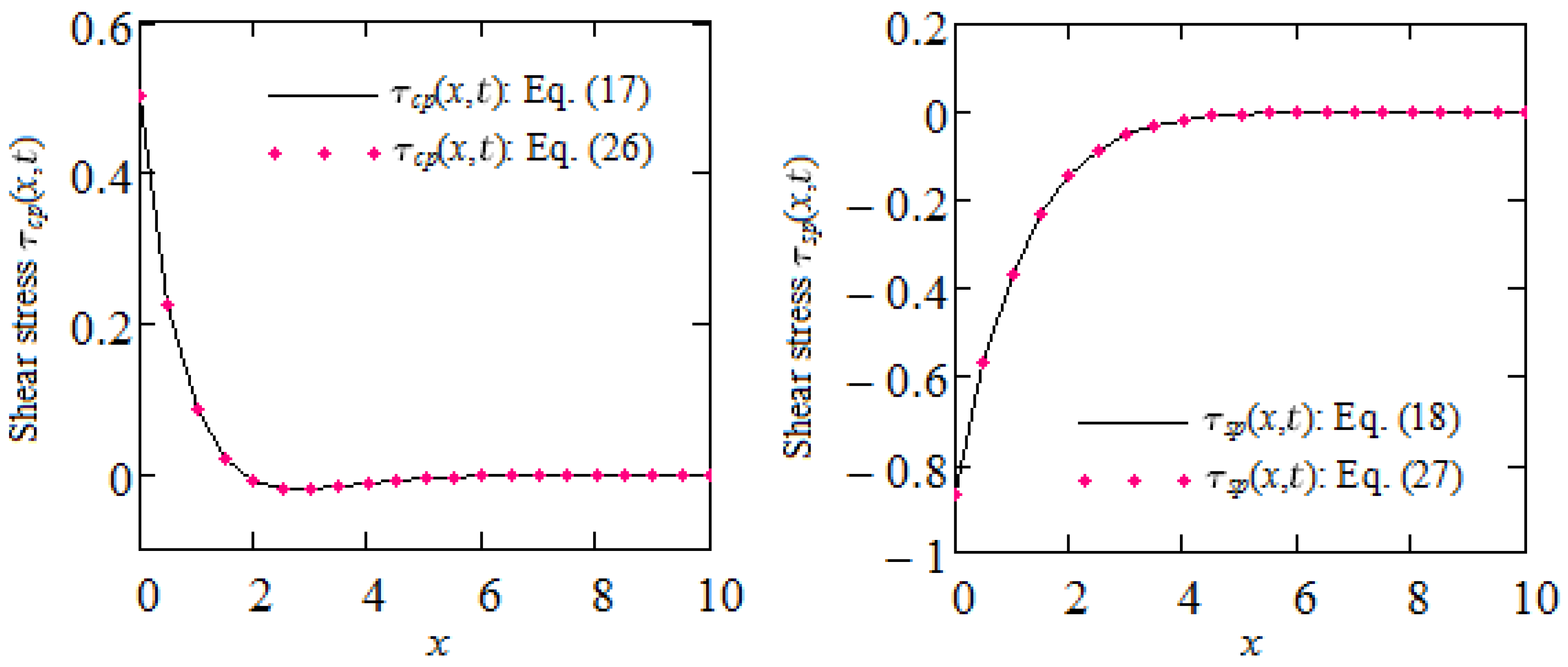
3.1. Exact Expressions for the Shear Stresses ${\tau }_{cp}(x,t)$, ${\tau }_{sp}(x,t)$

The dimensionless permanent shear stresses ${\tau }_{cp}(x,t)$ and ${\tau }_{sp}(x,t)$ corresponding to the two motions in discussion have to satisfy the governing Equation (13) and the boundary conditions (10). Lengthy but straightforward computations show that these shear stresses can be presented in simple forms

$${\tau }_{cp}(x,t)={\mathrm{e}}^{-mx}\cos (\omega t-nx); x>0, t\in R,$$

(17)

$${\tau }_{sp}(x,t)={\mathrm{e}}^{-mx}\sin (\omega t-nx); x>0, t\in R.$$

(18)

In the above relations, the non-dimensional constants m and n have the expressions

$$m=\sqrt{\frac{\omega }{2}}\sqrt{\frac{a\omega +\sqrt{{(a\omega )}^2+b^2}}{{(\gamma \omega )}^2+{(1-\delta {\omega }^2)}^2}}, n=\sqrt{\frac{\omega }{2}}\sqrt{\frac{-a\omega +\sqrt{{(a\omega )}^2+b^2}}{{(\gamma \omega )}^2+{(1-\delta {\omega }^2)}^2}},$$

(19)

$$a=\frac{\gamma {\omega }^2(1-\beta {\omega }^2+\alpha M)+(1-\delta {\omega }^2)[-\alpha {\omega }^2+(1-\beta {\omega }^2)M]}{{\omega }^2},$$

(20)

$$b=(1-\delta {\omega }^2)(1-\beta {\omega }^2+\alpha M)-\gamma [-\alpha {\omega }^2+(1-\beta {\omega }^2)M].$$

(21)

The first exact solution under the form (17) has been provided by Rajagopal [18] for the dimensional velocity of Stokes’ second problem corresponding to the second-grade fluids.

In order to determine equivalent expressions for these permanent shear stresses, we use the dimensionless complex shear stress

$${\tau }_p(x,t)={\tau }_{cp}(x,t)+i{\tau }_{sp}(x,t); x>0, t\in R,$$

(22)

where i is the complex unit. This complex shear stress has to satisfy the partial differential Equation (13) and the boundary conditions

$${\tau }_p(0,t)={\mathrm{e}}^{i\omega t}, \underset{x\to \infty }{\lim }{\tau }_p(x,t)=0; t\in R.$$

(23)

Because the governing Equation (13) is linear and the form of boundary conditions (23) is considered, we are in search of a solution with the following structure

$${\tau }_p(x,t)=T(x){\mathrm{e}}^{i\omega t}; x>0, t\in R,$$

(24)

where $T(\cdot )$ is an unknown function. Direct computations show that

$${\tau }_p(x,t)={\mathrm{e}}^{i\omega t-px}; x>0, t\in R,$$

(25)

while

$${\tau }_{cp}(x,t)=\mathrm{Re}\left\{{\mathrm{e}}^{i\omega t-px}\right\} ; x>0, t\in R,$$

(26)

$${\tau }_{sp}(x,t)=\mathrm{Im}\left\{{\mathrm{e}}^{i\omega t-px}\right\} ; x>0, t\in R.$$

(27)

In the above relations, the dimensionless constant p is defined by the equality

$$p=\sqrt{\frac{(1-\beta {\omega }^2+i\omega \alpha )(i\omega +M)}{1-\delta {\omega }^2+i\omega \gamma }}$$

(28)

and simple computations clearly show that ${\tau }_{cp}(x,t)$ and ${\tau }_{sp}(x,t)$ given by Equations (26) and (27) satisfy the governing Equation (13) and the boundary conditions (10).

The equivalence of their expressions given by Equations (17), (26) and (18), (27), respectively, is proved by means of Figure 1.

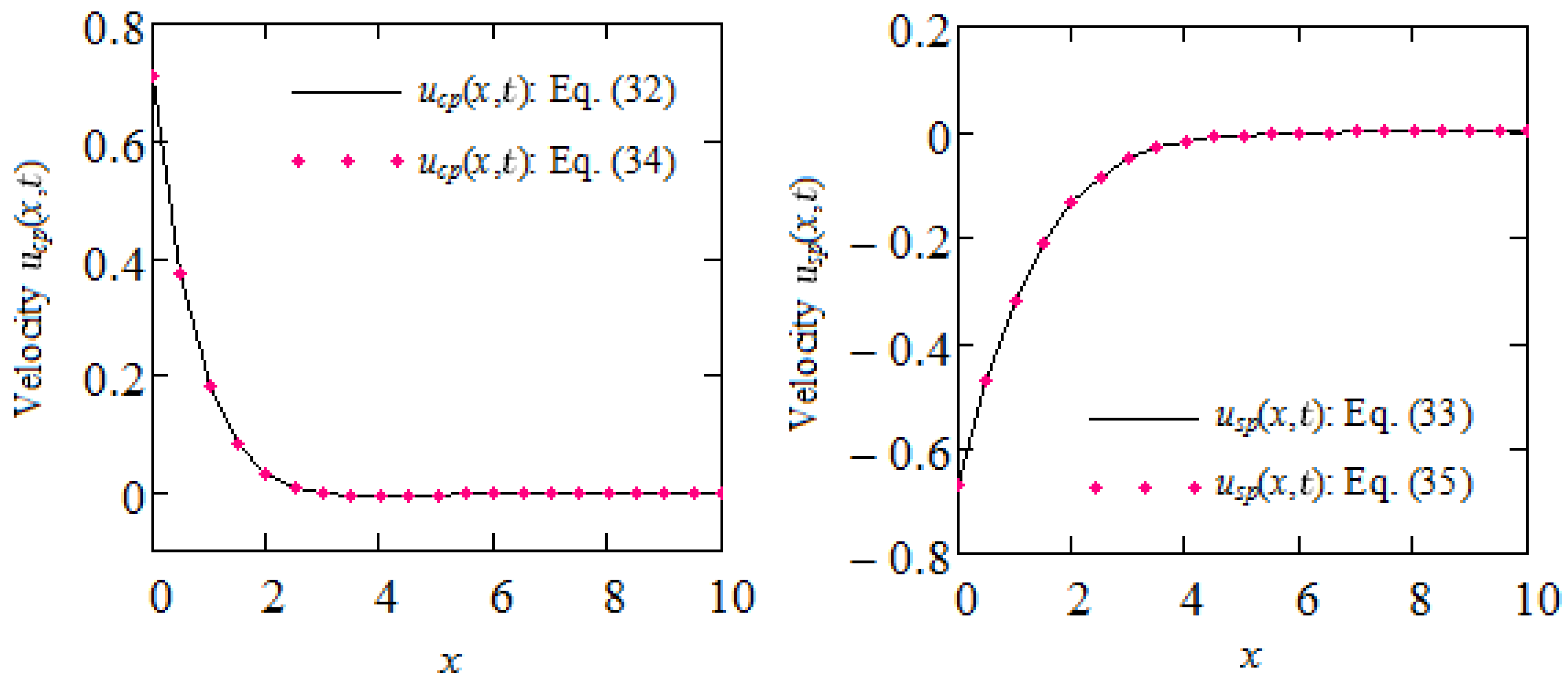
3.2. Exact Expressions for the Velocity Fields $u_{cp}(x,t)$, $u_{sp}(x,t)$

Once the permanent shear stresses ${\tau }_{cp}(x,t)$ and ${\tau }_{sp}(x,t)$ are known, we can determine the corresponding velocity fields $u_{cp}(x,t)$ and $u_{sp}(x,t)$. They have to satisfy the governing Equations (8) and (9) and the limiting condition (7). Bearing in mind the simple forms of ${\tau }_{cp}(x,t)$ and ${\tau }_{sp}(x,t)$ from Equations (17) and (18), we are looking for $u_{cp}(x,t)$ an expression of the form

$$u_{cp}(x,t)=\left[c\cos (\omega t-ny)+d\sin (\omega t-ny)\right] {\mathrm{e}}^{-mx}; x>0, t\in R.$$

(29)

Lengthy but straightforward computations show that $u_{cp}(x,t)$ from Equality (29) satisfies the governing Equation (9) if and only if

$$c=\frac{(1-\beta {\omega }^2)[\omega \gamma n-(1-\delta {\omega }^2)m]-\omega \alpha [\omega \gamma m+(1-\delta {\omega }^2)n]}{(m^2+n^2)[{(\omega \gamma )}^2+{(1-\delta {\omega }^2)}^2]}$$

(30)

$$d=-\frac{\omega \alpha [\omega \gamma n-(1-\delta {\omega }^2)m]+(1-\beta {\omega }^2)[\omega \gamma m+(1-\delta {\omega }^2)n}{(m^2+n^2)[{(\omega \gamma )}^2+{(1-\delta {\omega }^2)}^2]}$$

(31)

and

$$u_{cp}(x,t)=-\sqrt{c^2+d^2}{\mathrm{e}}^{-mx}\sin (\omega t-nx+\phi ); x>0, t\in R,$$

(32)

where $\phi =\mathrm{arctg}(c/d)$. Similar computations also show that

$$u_{sp}(x,t)=\sqrt{c^2+d^2}{\mathrm{e}}^{-mx}\cos (\omega t-nx+\phi ); x>0, t\in R.$$

(33)

Equivalent expressions for $u_{cp}(x,t)$ and $u_{sp}(x,t)$, namely

$$u_{cp}(x,t)=-\mathrm{Re}\left\{\left(\frac{p}{i\omega +M}\right){\mathrm{e}}^{i\omega t-px}\right\}; x>0, t\in R,$$

(34)

$$u_{sp}(x,t)=-\mathrm{Im}\left\{\left(\frac{p}{i\omega +M}\right){\mathrm{e}}^{i\omega t-px}\right\}; x>0, t\in R,$$

(35)

have been obtained by introducing ${\tau }_{cp}(x,t)$ and ${\tau }_{sp}(x,t)$ from the relations (26) and (27) in Equation (8). Simple computations show that $u_{cp}(x,t)$ and $u_{sp}(x,t)$ given by Equations (34) and (35) satisfy all governing Equations (8), (9) and (14). The equivalence of the expressions of $u_{cp}(x,t)$ and $u_{sp}(x,t)$ given by Equations (32), (34) and (33), (35), respectively, has been proved by means of Figure 2. Furthermore, it’s readily noticeable that the dimensionless permanent solutions, which correspond to identical movements of IGBFs when magnetic influences are absent, can be directly derived by setting $M=0$ in the overall solutions. These solutions, along with the previously mentioned ones, are new contributions within the existing body of literature.

4. Limiting Cases

As was already mentioned at the beginning of Section 2, similar solutions for incompressible Newtonian, second grade, Maxwell, Oldroyd-B, and Burgers’ fluids performing the same motions can be immediately obtained as limiting cases of the present solutions. In order to avoid repetition, we shall show this thing for the second-grade fluids because their constitutive equations cannot be obtained from those of IGBFs. However, for the present motions, the governing equations corresponding to these fluids can be obtained as limiting cases of present equations.

4.1. Case $\alpha =\beta =\delta =0$ (Permanent Solutions for Second-Grade Fluids)

Making $\alpha =\beta =\delta =0$ in Equations (17), (18), (26) and (27), one finds the following equivalent expressions,

$${\tau }_{SGcp}(x,t)={\mathrm{e}}^{-m_{1}x}\cos (\omega t-n_{1}x); x>0, t\in R,$$

(36)

$${\tau }_{SGsp}(x,t)={\mathrm{e}}^{-m_{1}x}\sin (\omega t-n_{1}x); x>0, t\in R$$

(37)

Respectively,

$${\tau }_{SGcp}(x,t)=\mathrm{Re}\left\{{\mathrm{e}}^{i\omega t-p_{1}x}\right\} ; x>0, t\in R,$$

(38)

$${\tau }_{SGsp}(x,t)=\mathrm{Im}\left\{{\mathrm{e}}^{i\omega t-p_{1}x}\right\} ; x>0, t\in R,$$

(39)

for the dimensionless permanent shear stresses ${\tau }_{SGcp}(x,t)$ and ${\tau }_{SGsp}(x,t)$. They correspond to unsteady MHD motions of the incompressible second-grade fluids over an infinite plate that applies the oscillatory shear stresses $S\cos (\omega t)$ or $S\sin (\omega t)$ to the fluid. The expressions of these solutions are identical to those obtained by Fetecau and Morosanu [19] in which $K=0$ (i.e., in the absence of porous effects). In the above relations, the new constants $m_1, n_1$, and $p_1$ are given by the relations

$$m_1=\sqrt{\frac{\omega }{2}}\sqrt{\frac{a_1\omega +\sqrt{{(a_1\omega )}^2+b_1^2}}{1+{(\gamma \omega )}^2}}, n_1=\sqrt{\frac{\omega }{2}}\sqrt{\frac{-a_1\omega +\sqrt{{(a_1\omega )}^2+b_1^2}}{1+{(\gamma \omega )}^2}}, p_1=\sqrt{\frac{i\omega +M}{1+i\omega \gamma },}$$

(40)

in which

$$a_1=\gamma +\frac{M}{{\omega }^2} \mathrm{and} b_1=1-\gamma M.$$

Taking now $\alpha =\beta =\delta =0$ in the Equations (32)–(35), one obtains the corresponding permanent velocity fields

$$u_{SGcp}(x,t)=-\sqrt{c_1^2+d_1^2}{\mathrm{e}}^{-m_{1}x}\sin (\omega t-n_{1}x+{\phi }_1); x>0, t\in R,$$

(41)

$$u_{SGsp}(x,t)=\sqrt{c_1^2+d_1^2}{\mathrm{e}}^{-m_{1}x}\cos (\omega t-n_{1}x+{\phi }_1); x>0, t\in R,$$

(42)

$$u_{SGcp}(x,t)=-\mathrm{Re}\left\{\left(\frac{p_1}{i\omega +M}\right){\mathrm{e}}^{i\omega t-p_{1}x}\right\}; x>0, t\in R,$$

(43)

$$u_{SGsp}(x,t)=-\mathrm{Im}\left\{\left(\frac{p_1}{i\omega +M}\right){\mathrm{e}}^{i\omega t-p_{1}x}\right\}; x>0, t\in R,$$

(44)

in which

$$c_1=\frac{\omega \gamma n_1-m_1}{(m_1^2+n_1^2)[{(\omega \gamma )}^2+1]}, d_1=\frac{\omega \gamma m_1+n_1}{(m_1^2+n_1^2)[{(\omega \gamma )}^2+1]}, {\phi }_1=\mathrm{arctg}\left(\frac{\omega \gamma n_1-m_1}{\omega \gamma m_1+n_1}\right).$$

(45)

Simple computations show that the expressions of $u_{SGcp}(x,t),$ $u_{SGsp}(x,t)$ from Equations (43) and (44) are identical to those obtained by Fetecau and Morosanu [19] in their Equation (61). In exchange, the expressions of these entities from Equations (41) and (42) have different forms from those from the above-mentioned reference. However, they are equivalent by transitivity. Baranovskii [20,21] has recently obtained interesting results concerning the movement of incompressible second-grade fluids within rectangular regions.

4.2. Case $\alpha =\beta =\gamma =\delta =0$ (Permanent Solutions for Newtonian Fluids)

Taking $\alpha =\beta =\gamma =\delta =0$ in Equations (17), (18), (32) and (33) or $\gamma =0$ in Equations (36), (37), (41) and (42), the similar solutions

$${\tau }_{Ncp}(x,t)={\mathrm{e}}^{-qx}\cos (\omega t-rx); x>0, t\in R,$$

(46)

$${\tau }_{Nsp}(x,t)={\mathrm{e}}^{-qx}\sin (\omega t-rx); x>0, t\in R,$$

(47)

$$u_{Ncp}(x,t)=-\frac{1}{\sqrt[4]{M^2+{\omega }^2}}{\mathrm{e}}^{-qx}\sin (\omega t-rx+\psi ); x>0, t\in R,$$

(48)

$$u_{Nsp}(x,t)=\frac{1}{\sqrt[4]{M^2+{\omega }^2}}{\mathrm{e}}^{-qx}\cos (\omega t-rx+\psi ); x>0, t\in R,$$

(49)

corresponding to the identical movements of incompressible Newtonian fluids are acquired. Here, the constants q, r and $\psi$ are given by the relations

$$q=\sqrt{\frac{M+\sqrt{M^2+{\omega }^2}}{2}}, r=\sqrt{\frac{-M+\sqrt{M^2+{\omega }^2}}{2}}, \psi =\mathrm{arctg}\left(\frac{M+\sqrt{M^2+{\omega }^2}}{\omega }\right).$$

(50)

The equivalent expressions of these entities have also simple forms, namely

$${\tau }_{Ncp}(x,t)=\mathrm{Re}\left\{{\mathrm{e}}^{i\omega t-x\sqrt{i\omega +M}}\right\}; x>0, t\in R,$$

(51)

$${\tau }_{Nsp}(x,t)=\mathrm{Im}\left\{{\mathrm{e}}^{i\omega t-x\sqrt{i\omega +M}}\right\}; x>0, t\in R,$$

(52)

$$u_{Ncp}(x,t)=-\mathrm{Re}\left\{\frac{1}{\sqrt{i\omega +M}}{\mathrm{e}}^{i\omega t-x\sqrt{i\omega +M}}\right\}; x>0, t\in R,$$

(53)

$$u_{Nsp}(x,t)=-\mathrm{Im}\left\{\frac{1}{\sqrt{i\omega +M}}{\mathrm{e}}^{i\omega t-x\sqrt{i\omega +M}}\right\}; x>0, t\in R.$$

(54)

Finally, it is interesting to observe that in the absence of magnetic effects, the expressions of ${\tau }_{Ncp}(x,t)$ and ${\tau }_{Nsp}(x,t)$ from the Equations (46) and (47), respectively, are identical to the dimensionless forms of the velocity fields obtained by Erdogan [22] in the relations (12) and (17). This is possible since the shear stress in the present case and the fluid velocity in Erdogan’s paper satisfy the same governing equations and boundary conditions.

4.3. The Case $\omega =0$ (the Plate Applies a Constant Shear Stress S to the Fluid)

Making $\omega =0$ in the relations (26) and (34) or (51) and (53) one finds the expressions of dimensionless permanent shear stress and velocity fields

$${\tau }_{Cp}(x)={\mathrm{e}}^{-x\sqrt{M}}; x>0, t\in R,$$

(55)

$$u_{Cp}(x)=-\frac{1}{\sqrt{M}}{\mathrm{e}}^{-x\sqrt{M}}; x>0, t\in R,$$

(56)

corresponding to the unsteady motion of IGBFs over an infinite flat plate that applies a constant shear stress S to the fluid. As it was to be expected, these expressions are the same both for Newtonian and non-Newtonian fluids. This is not a surprise because, as it results from the literature [23], the non-Newtonian effects disappear in time.

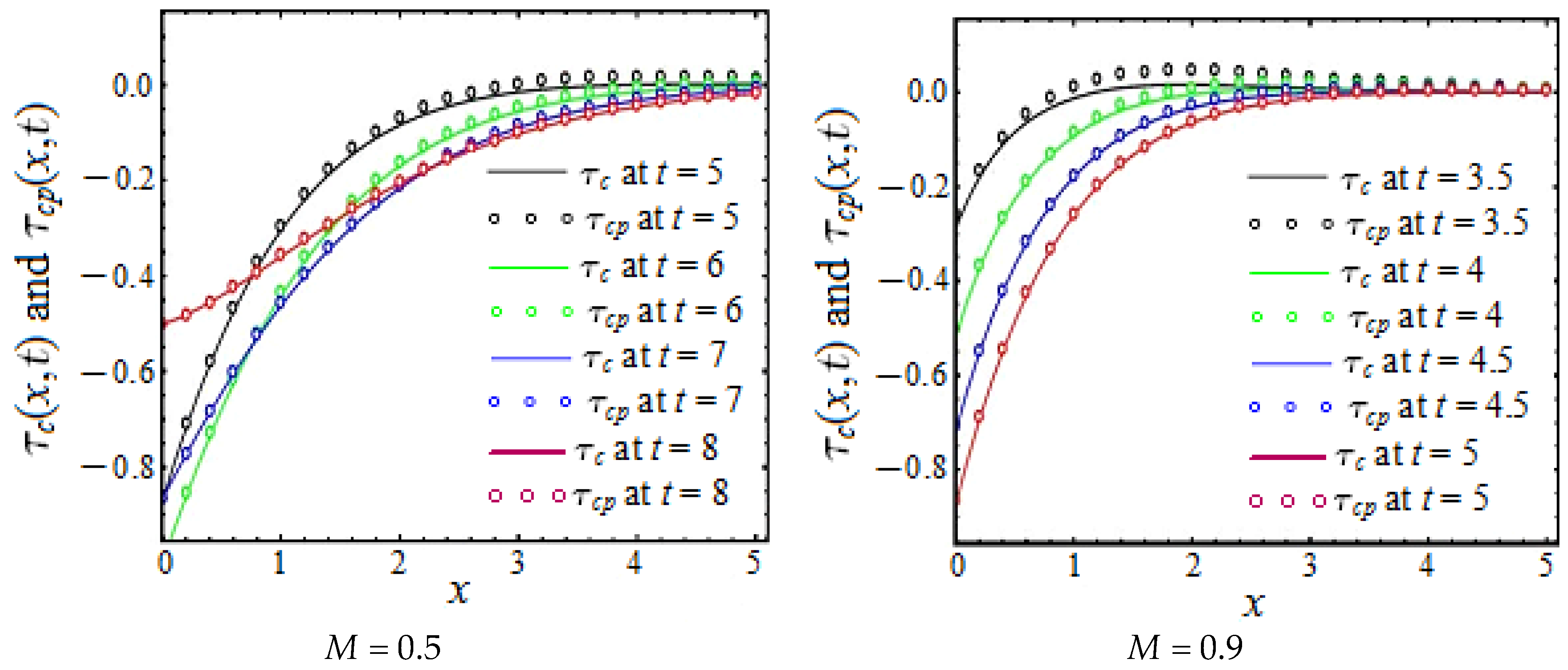
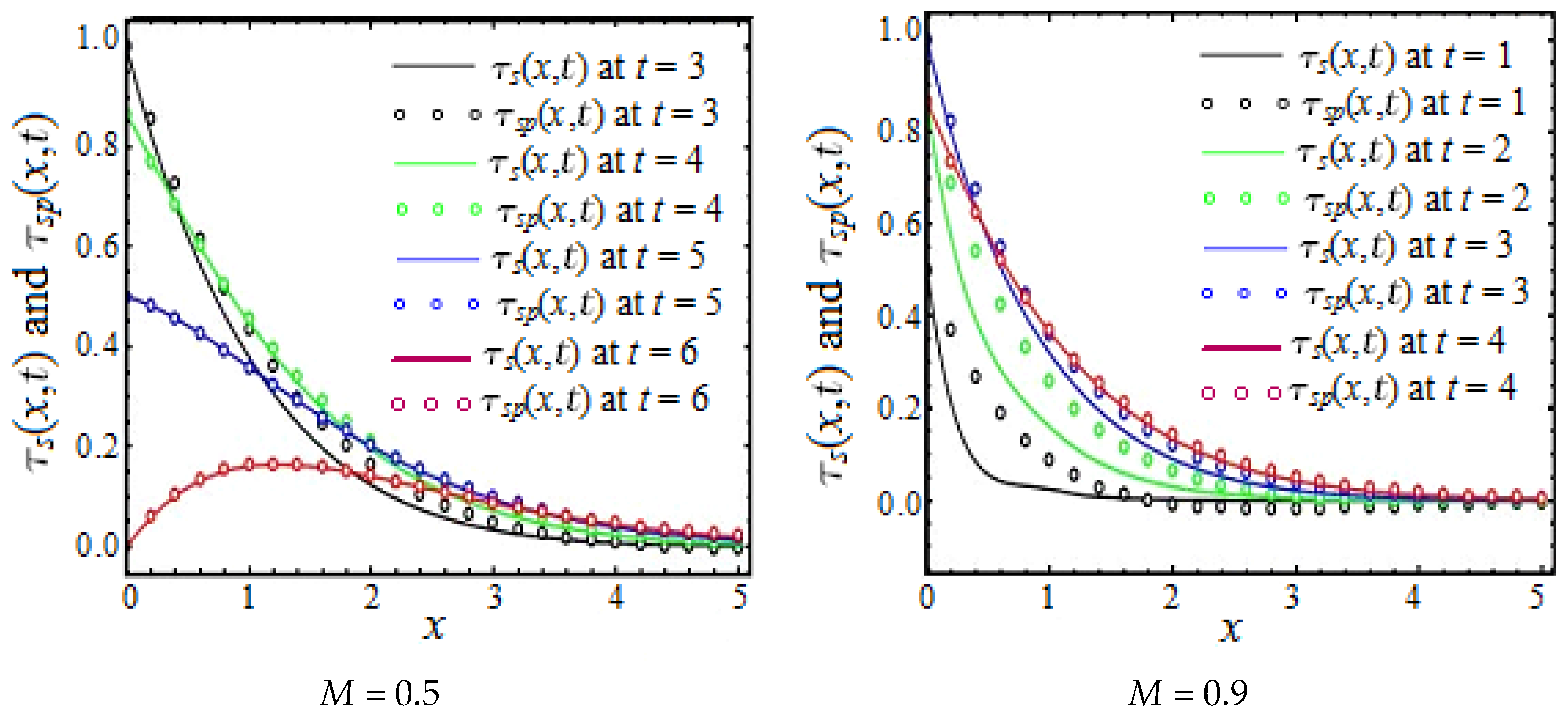
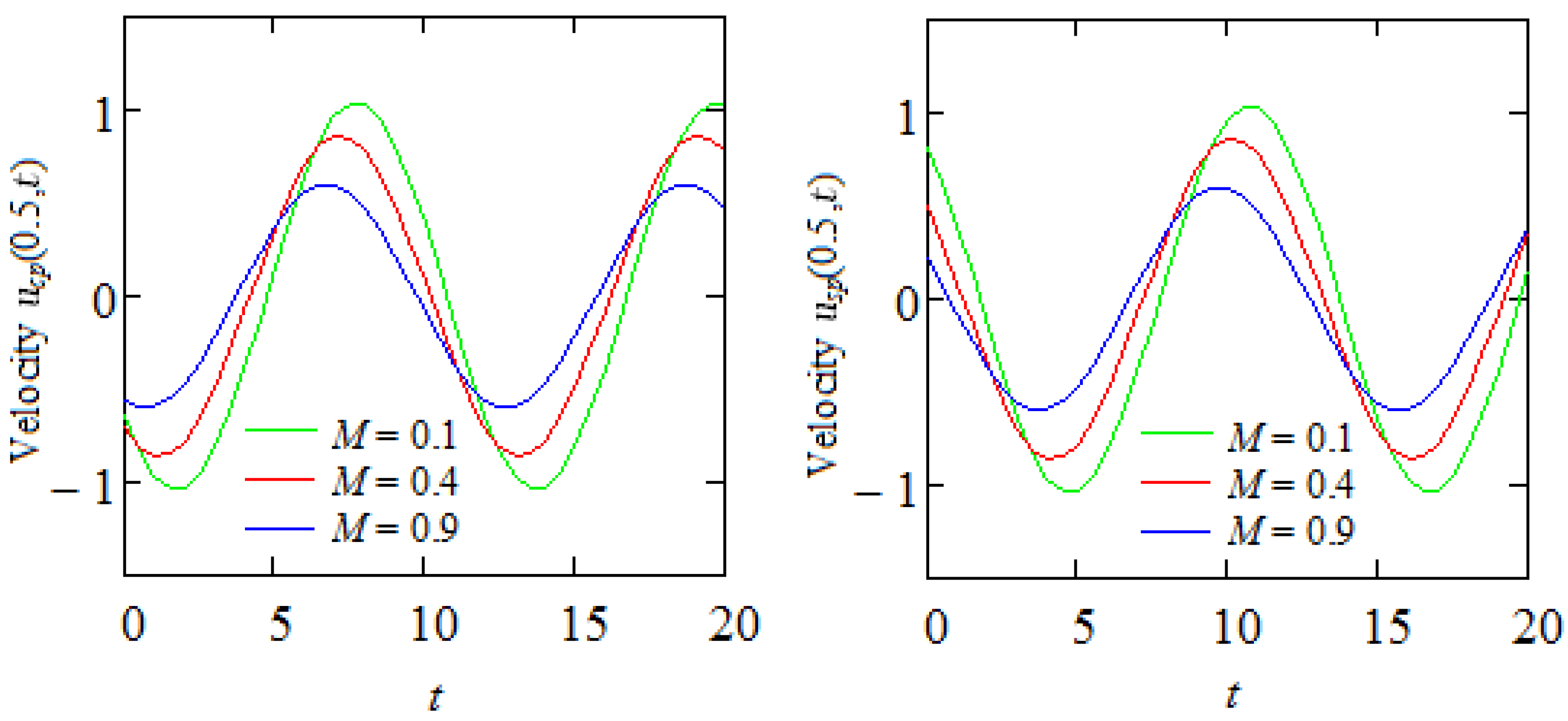
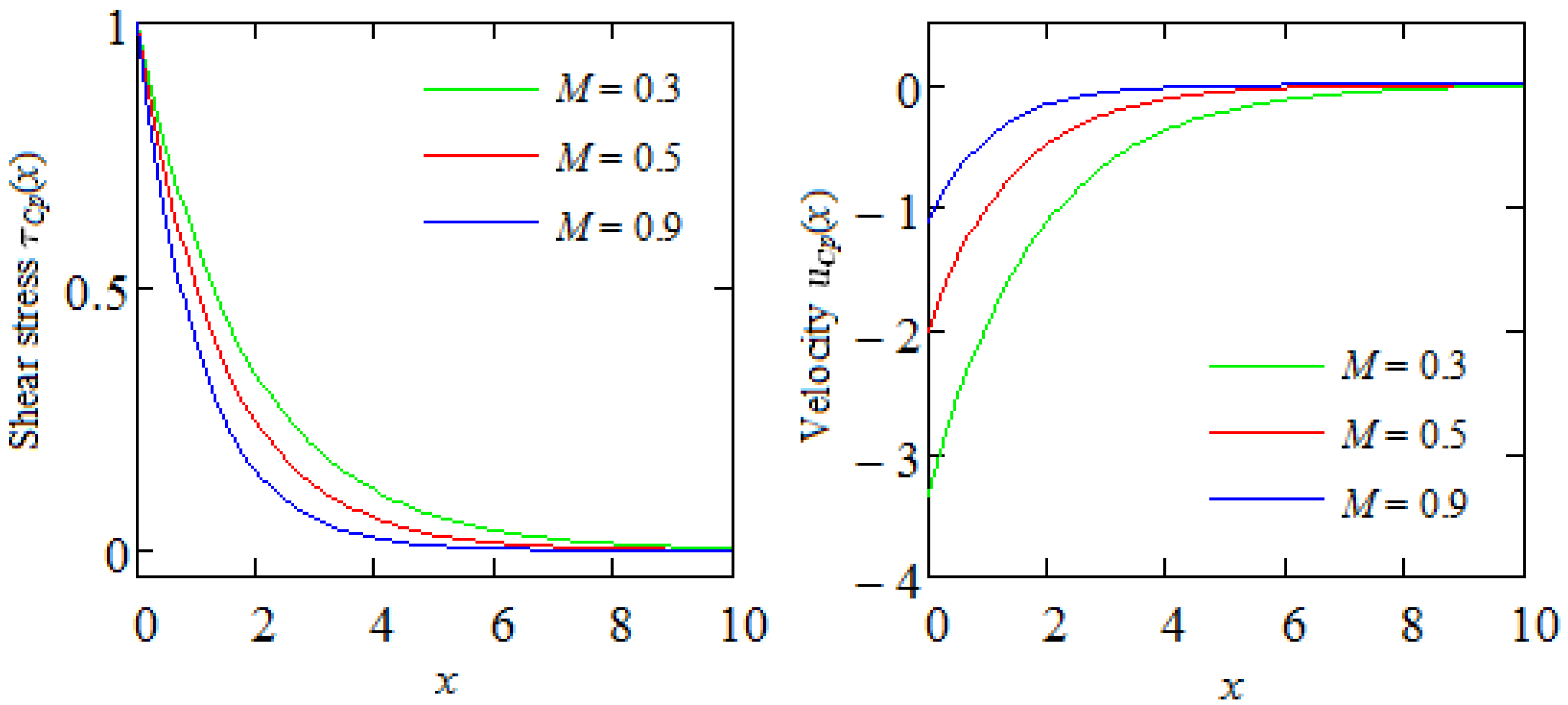
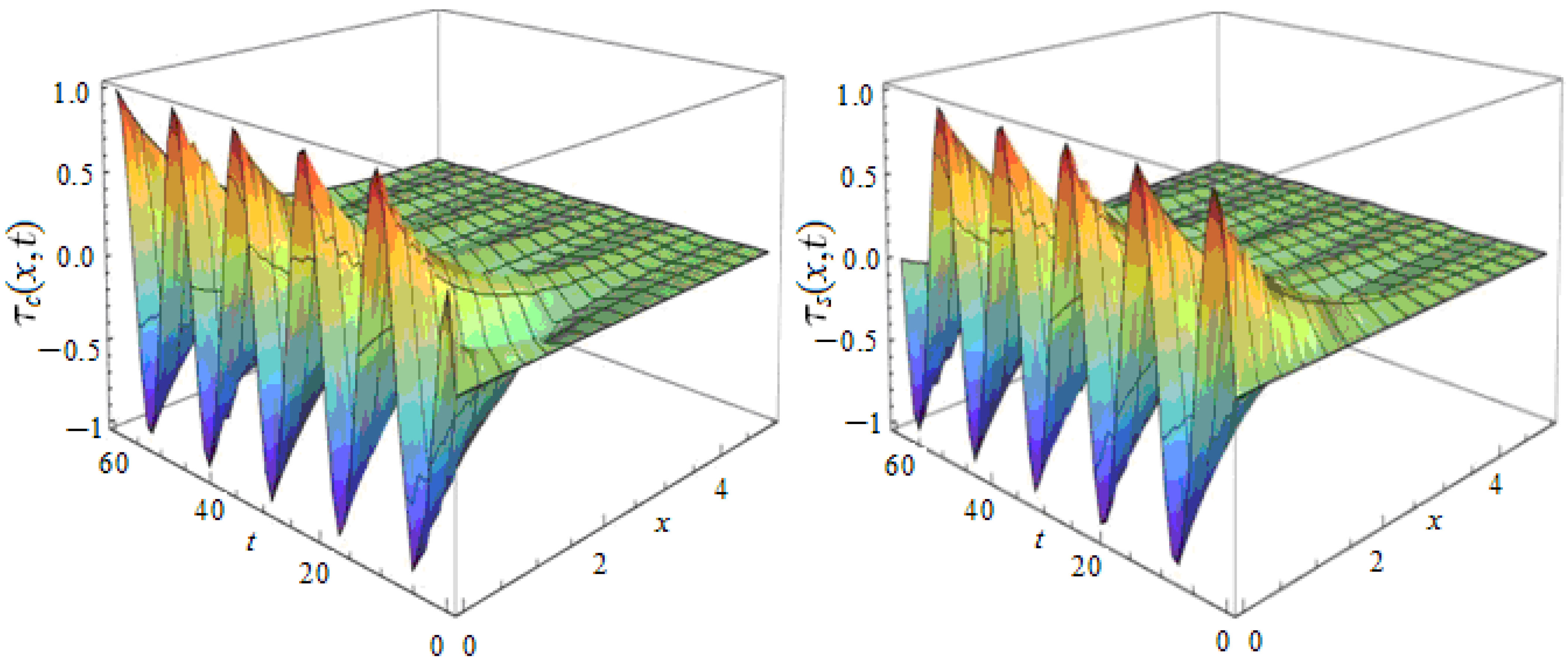
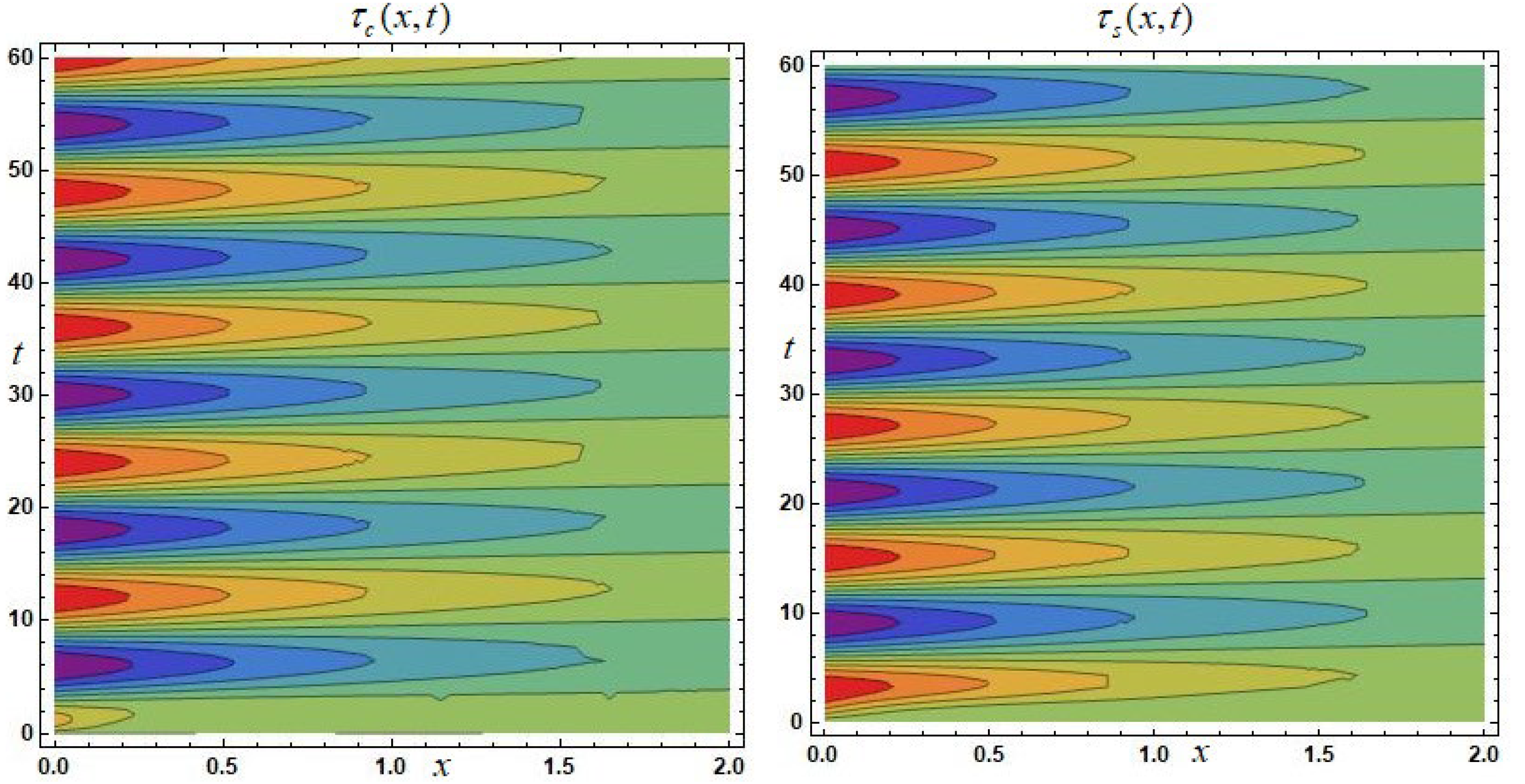
5. Some Numerical Results and Conclusions

The present study offers closed-form analytical expressions for dimensionless steady-state velocities and non-null shear stress distributions that pertain to isothermal MHD unsteady flows of IGBFs above an infinite flat plate subject to oscillatory shear stress conditions. The obtained solutions also encompass scenarios where the motion arises from a constant shear stress applied at the boundary, thus serving as a limiting case. Collectively, these solutions stand as the inaugural exact derivations for MHD flow behaviors exhibited by such fluids, particularly in scenarios where the shear stress is prescribed at the boundary. Moreover, these formulations can readily be tailored to yield solutions for other fluid models, such as Burgers’, Oldroyd-B, Maxwell, second grade, and Newtonian, all engaging in the same underlying motions. Notably, these derivations recover well-established solutions pertaining to second-grade fluids as limiting instances. Furthermore, akin solutions describing the identical motions of IGBFs sans the influence of magnetic effects can similarly be derived as limiting cases within the broader framework of these general solutions. These findings, noteworthy for their novelty, contribute novel insights to the existing body of scientific literature.

To validate the derived outcomes, we presented all solutions in two distinct formats, with their equivalence being visually demonstrated. In addition, as was to be expected, Figure 3 and Figure 4 clearly show that the starting solutions ${\tau }_c(x,t)$ and ${\tau }_s(x,t)$ (numerical solutions) converge to the corresponding permanent solutions ${\tau }_{cp}(x,t)$ and ${\tau }_{sp}(x,t)$, respectively, for increasing values of the time t.

From these graphical illustrations, which have been generated for two different values of the magnetic parameter M, it can be inferred that the time required to attain the permanent state diminishes as the magnetic parameter M increases. Consequently, the presence of a magnetic field leads to an earlier achievement of the permanent state for these unsteady motions of IGBFs. In addition, the required time to touch the permanent state for motions due to sine oscillations is shorter than that for cosine oscillations of shear stress on the boundary.

Now, in order to bring to light some characteristics of the fluid motion, Figure 5 and Figure 6 have been included here. Figure 5, which presents the time variations of the permanent velocities $u_{cp}(x,t)$ and $u_{sp}(x,t)$ at the middle of the channel for increasing values of the magnetic parameter M, shows that the oscillations’ amplitude decreases in the presence of a magnetic field. Moreover, the oscillatory characteristic feature of the two movements, along with the phase discrepancy between them, can be readily noticed.

Figure 6 shows the influence of the same parameter M on the dimensionless permanent solutions ${\tau }_{Cp}(x)$ and $u_{Cp}(x)$ corresponding to the unsteady MHD motion of IGBFs induced by the flat plate that applies a constant shear stress S to the fluid. It results in both the fluid velocity absolute value and the shear stress decline for increasing values of the magnetic parameter M. Consequently, the fluid moves slower in the presence of a magnetic field.

Finally, for comparison, the spatial profiles of the dimensionless starting shear stresses ${\tau }_c(x,t)$ and ${\tau }_s(x,t)$ (numerical solutions) are depicted adjoining in Figure 7 for $\alpha =0.8,$ $\beta =0.5, \gamma =0.7, \delta =0.4, \omega =\pi /6$ and $M=0.9$. As before, the oscillatory behavior and the phase difference between the two motions are easily observed and the initial and boundary conditions are clearly satisfied. The three-dimensional pattern of the initial shear stresses for both cases is also depicted using two-dimensional contour plots [24] in Figure 8. This visualization is based on the same set of physical parameter values. Different colors are used to indicate their trajectories. The red and purple colors are used to bring to light the solutions’ maximum and minimum values, respectively. The oscillatory behavior of the solutions is indicated by the alternation of two distinct sets of almost closed trajectories throughout the time t. The increasing values of x lead to a decrease in the oscillation amplitude.

The main results obtained through this study are:

(1)

Concise analytical expressions have been provided for the dimensionless permanent solutions associated with unsteady MHD motions of IGBFs over an unbounded flat plate that applies oscillatory or constant shear stresses upon the fluid;

(2)

These expressions can be promptly tailored to yield comparable solutions for incompressible Burgers’, Oldroyd-B, Maxwell, second grade, and Newtonian fluids performing the same motions, and their correctness has been graphically proved;

(3)

The acquired outcomes have been employed in investigating the magnetic effects on both the steady state and fluid velocity. It was found that the permanent state is more quickly obtained, and the fluid velocity is diminished in the presence of a magnetic field;

(4)

It is pertinent to highlight that the governing Equation (14), which characterizes shear stress, exhibiting an analogous structure to Equation (13) delineating velocity, assumes pivotal significance in obtaining new exact solutions for MHD motions of IGBFs.

References

1. Fetecau, C.; Hayat, T.; Corina, F. Seady-state solutions for some simple flows of generalized Burgers fluids. Int. J. Non-Linear Mech. 2006, 41, 880–887. [Google Scholar] [CrossRef]
2. Tong, D.; Shan, L. Exact solutions for generalized Burgers’ fluid in an annular pipe. Meccanica 2009, 44, 427–431. [Google Scholar] [CrossRef]
3. Zheng, L.C.; Zhao, F.F.; Zhang, X.X. An exact solution for an unsteady flow of a generalized Burgers’ fluid induced by an accelerating plate. Int. J. Nonlinear Sci. Numer. Simul. 2010, 11, 457–464. [Google Scholar] [CrossRef]
4. Tong, D. Starting solutions for oscillating motions of a generalized Burgers’ fluid in cylindrical domains. Acta Mech. 2010, 214, 395–407. [Google Scholar] [CrossRef]
5. Jamil, M. First problem of Stokes for generalized Burgers’ fluids. Int. Sch. Res. Not. 2012, 2012, 831063. [Google Scholar] [CrossRef]
6. Khan, I.; Hussanan, A.; Salleh, M.Z.; Tahar, R.M. Exact solutions of accelerated flows for a generalized Burgers’ fluid, I: The case. In Proceedings of the 4th International Conference on Computer Science and Computational Mathematics (ICCSCM 2015), Langkawi, Malaysia, 7–8 May 2015; pp. 47–52. [Google Scholar]
7. Fetecau, C.; Corina, F.; Akhtar, S. Permanent solutions for some axial motions of generalized Burgers fluids in cylindrical domains. Ann. Acad. Rom. Sci. Ser. Math. Appl. 2015, 7, 271–284. [Google Scholar]
8. Sultan, Q.; Nazar, M.; Ali, U.; Ahmad, I. On the flow of generalized Burgers’ fluid induced by sawtooth pulses. J. Appl. Fluid Mech. 2015, 8, 243–254. [Google Scholar] [CrossRef]
9. Khan, M.; Malik, R.; Anjum, A. Exact solutions of MHD second Stokes’ flow of generalized Burgers fluid. Appl. Math. Mech. 2015, 36, 211–224. [Google Scholar] [CrossRef]
10. Abro, K.A.; Hussain, M.; Baig, M.M. Analytical solution of magnetohydrodynamics generalized Burgers’ fluid embedded with porosity. Int. J. Adv. Appl. Sci. 2017, 4, 80–89. [Google Scholar] [CrossRef]
11. Alqahtani, A.M.; Khan, I. Time-dependent MHD flow of non-Newtonian generalized Butgers’ fluid (GBF) over a suddenly moved plate with generalized Darcy’s law. Front. Phys. 2020, 7, 214. [Google Scholar] [CrossRef]
12. Hussain, M.; Qayyum, M.; Sidra, A. Modeling and analysis of MHD oscillatory flows of generalized Burgers’ fluid in a porous medium using Fourier transform. J. Math. 2022, 2022, 2373084. [Google Scholar] [CrossRef]
13. Renardy, M. Inflow boundary condition for steady flow of viscoelastic fluids with differential constitutive laws. Rocky Mt. J. Math. 1988, 18, 445–453. Available online: http://www.jstor.org/stable/44237133 (accessed on 30 August 2023). [CrossRef]
14. Renardy, M. An alternative approach to inflow boundary conditions for Maxwell fluids in three space dimensions. J. Non-Newton. Fluid Mech. 1990, 36, 419–425. [Google Scholar] [CrossRef]
15. Renardy, M. Recent advances in the mathematical theory of steady flow of viscoelastic fluids. J. Non-Newton. Fluid Mech. 1988, 1, 11–24. [Google Scholar] [CrossRef]
16. Rajagopal, K.R. A new development and interpretation of the Navier-Stokes fluid which reveals why the “Stokes Assumption” is inapt. Int. J. Non-Linear Mech. 2013, 50, 141–151. [Google Scholar] [CrossRef]
17. Cramer, K.R.; Pai, S.I. Magnetofluid Dynamics for Engineers and Applied Physicists; McGraw-Hill: New York, NY, USA, 1973. [Google Scholar]
18. Rajagopal, K.R. A note on unsteady unidirectional flows of a non-Newtonian fluid. Int. J. Non-Linear Mech. 1982, 17, 369–373. [Google Scholar] [CrossRef]
19. Fetecau, C.; Morosanu, C. Influence of magnetic field and porous medium on the steady state and flow resistance of second grade fluids on an infinite plate. Symmetry 2023, 15, 1269. [Google Scholar] [CrossRef]
20. Baranovskii, E.S.; Artemov, M.A. Steady flows of second grade fluids in a channel. Vestn. St. Petersburg Univ. Appl. Math. Comput. Sci. Control Process 2017, 13, 342–353. (In Russian) [Google Scholar] [CrossRef]
21. Baranovskii, E.S.; Artemov, M.A. Steady flows of second grade fluids subject to stick-slip boundary conditions. In Proceedings of the 23rd International Conference Engineering Mechanics, Svratka, Czech Republic, 15–18 May 2017; pp. 110–113. [Google Scholar]
22. Erdogan, M.E. A note on an unsteady flow of a viscous fluid due to an oscillating plane wall. Int. J. Non-Linear Mech. 2000, 35, 1–6. [Google Scholar] [CrossRef]
23. Joseph, D.D. Fluid Dynamics of Viscoelastic Liquids; Springer: New York, NY, USA, 1990. [Google Scholar]
24. Fullard, L.A.; Wake, G.C. An analytical series solution to the steady laminar flow of a Newtonian fluid in a partially filled pipe, including the velocity distribution and the dip phenomenon. IMA J. Appl. Math. 2015, 80, 1890–1901. [Google Scholar] [CrossRef]
Figure 1. Diagrams of shear stresses τ c p ( x , t ) and τ s p ( x , t ) given by Equations (17), (26) and (18), (27), respectively, for α = 0.8 ,     β = 0.5 ,     γ = 0.7 ,   δ = 0.4 ,     ω = π / 6 ,     M = 0.9 and t = 10 .
Symmetry 15 01683 g001
Figure 2. Diagrams of the velocities u c p ( x , t ) and u s p ( x , t ) given by Equations (32), (34) and (33), (35), respectively, for α = 0.8 ,     β = 0.5 ,     γ = 0.7 ,   δ = 0.4 ,     ω = π / 6 ,     M = 0.9 and t = 10 .
Symmetry 15 01683 g002
Figure 3. Convergence of the starting shear stress τ c ( x , t ) (numerical solution) to its permanent component τ c p ( x , t ) for α = 0.8 ,     β = 0.5 ,     γ = 0.7 ,   δ = 0.4 ,     ω = π / 6 , two values of M and increasing values of the time t.
Symmetry 15 01683 g003
Figure 4. Convergence of the starting shear stress τ s ( x , t ) (numerical solution) to its permanent component τ s p ( x , t ) for α = 0.8 ,     β = 0.5 ,     γ = 0.7 ,   δ = 0.4 ,     ω = π / 6 , two values of M and increasing values of the time t.
Symmetry 15 01683 g004
Figure 5. The time variations of the midplane permanent velocities u c p ( 0.5 , t ) and u s p ( 0.5 , t ) for α = 0.8 ,     β = 0.5 ,     γ = 0.7 ,     δ = 0.4 ,     ω = π / 6 ,     x = 0.5 and three values of M.
Symmetry 15 01683 g005
Figure 6. Configurations of the permanent shear stress and velocity fields τ C p ( x ) and u C p ( x ) given by Equations (55) and (56), respectively, for three values of M.
Symmetry 15 01683 g006
Figure 7. Spatial profiles of the starting shear stresses τ c ( x , t ) and τ s ( x , t ) (numerical solutions) for α = 0.8 ,     β = 0.5 ,     γ = 0.7 ,   δ = 0.4 ,     ω = π / 6 , and M = 0.9 .
Symmetry 15 01683 g007
Figure 8. Contour profiles of the starting shear stresses τ c ( x , t ) and τ s ( x , t ) (numerical solutions) for α = 0.8 ,     β = 0.5 ,     γ = 0.7 ,   δ = 0.4 ,     ω = π / 6 and M = 0.9 .
Symmetry 15 01683 g008
Disclaimer/Publisher’s Note: The statements, opinions and data contained in all publications are solely those of the individual author(s) and contributor(s) and not of MDPI and/or the editor(s). MDPI and/or the editor(s) disclaim responsibility for any injury to people or property resulting from any ideas, methods, instructions or products referred to in the content.