
Multiple Axes of Visual Symmetry: Detection and Aesthetic Preference
Abstract
:1. Introduction
2. Experiment 1
2.1. Materials and Methods
2.1.1. Participants
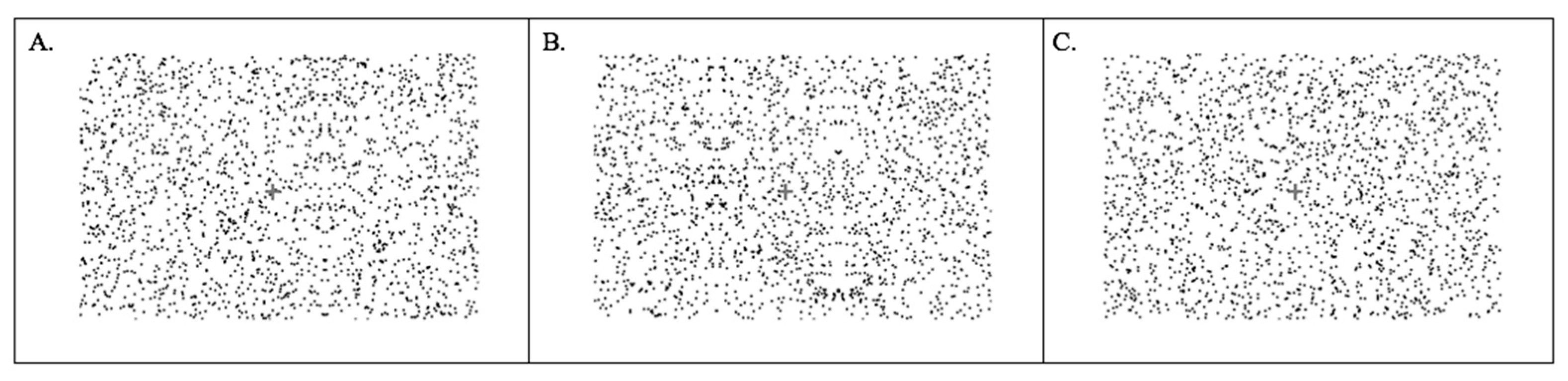
2.1.2. Apparatus and Stimuli
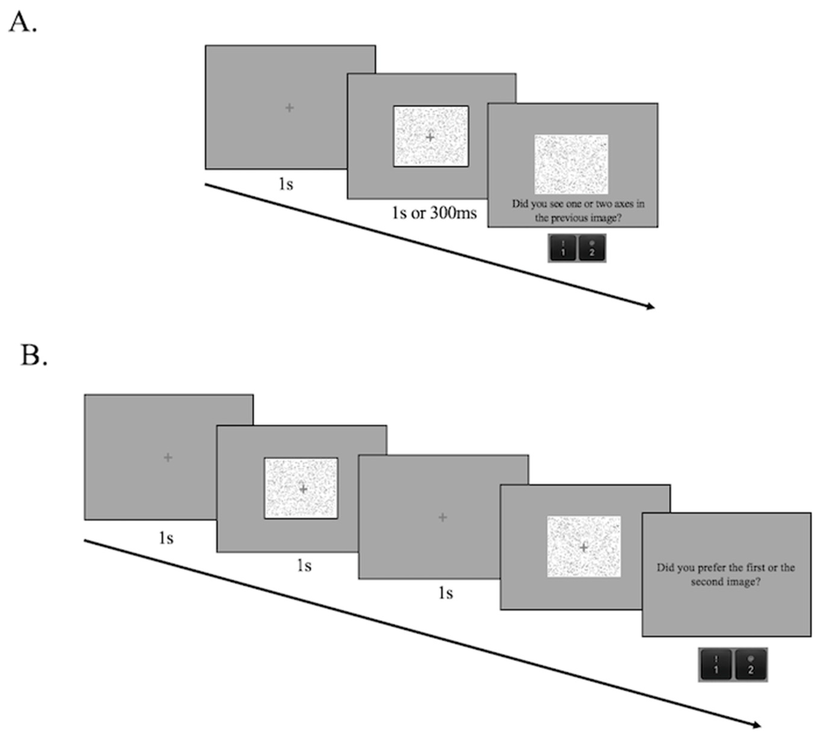
2.1.3. Procedure
2.1.4. Data Analysis
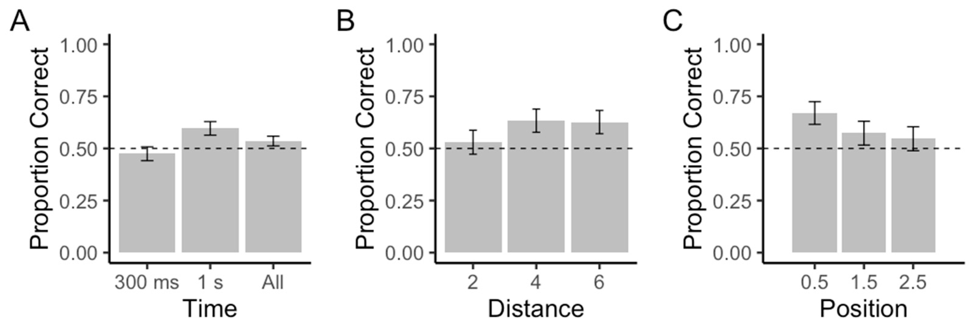
2.2. Results
2.3. Discussion
3. Experiment 2
3.1. Materials and Methods
3.1.1. Participants
3.1.2. Apparatus and Stimuli
3.1.3. Procedure
3.1.4. Data Analysis
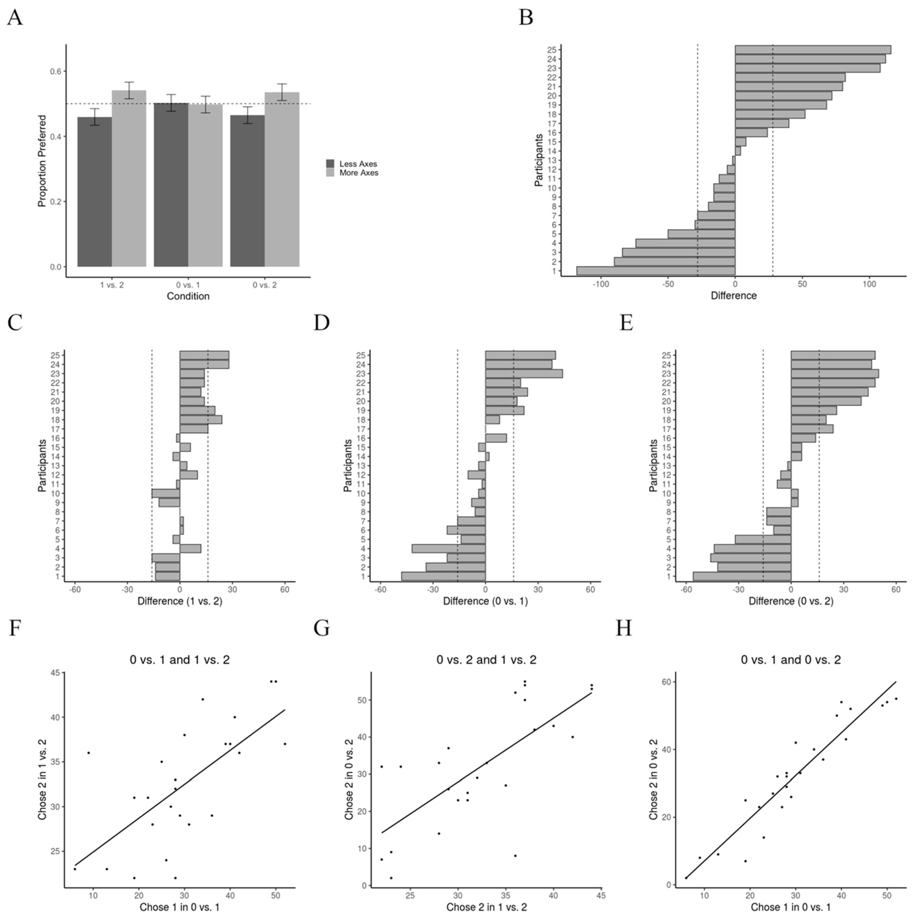
3.2. Results
3.3. Discussion
4. A Theoretical Framework for the Detection and Preference of Multiple-Symmetry Axes
4.1. Assumptions
- Seeing symmetry is detecting at least one axis of symmetry, and sensing more axes makes no difference.
- As the number of axes of symmetry increases, the probability of detecting at least one of them also increases. Thus, the probability of detecting at least one axis of symmetry follows probability summation [42].
- When confronted with a choice between symmetry or complexity, each individual has a consistent preference for either the former or latter. However, these judgments are likely influenced by noise, ranging from the nature of the stimuli to decision noise, and thus are not absolute.
- If an individual fails to detect symmetry in the two experimental images, preference is random.
4.2. Experiment 3—Test of the Assumptions of the Theoretical Framework
4.2.1. Methods
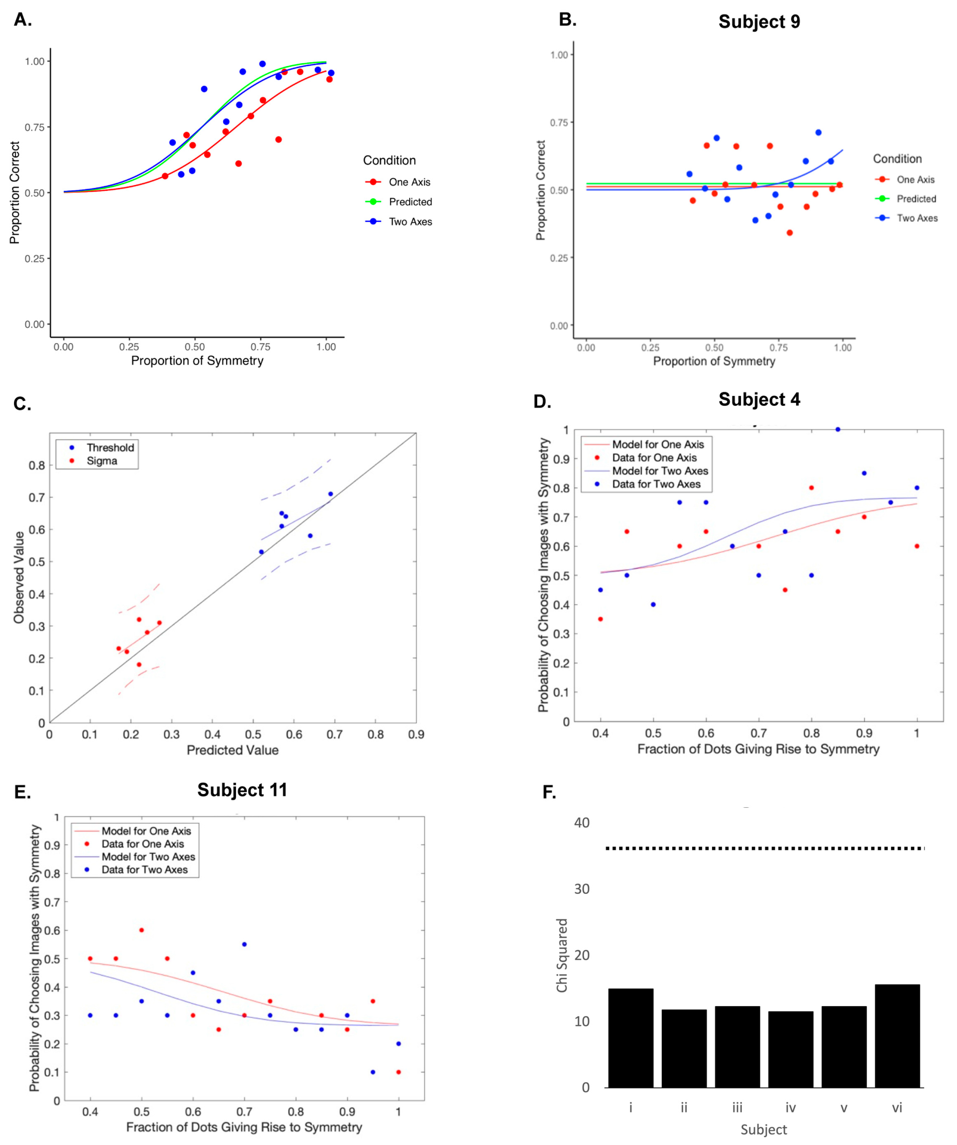
4.2.2. Results
4.2.3. Discussion
4.3. Computational Model for Individual Observers
4.3.1. Rationale
4.3.2. Fundamental Equations of the Model
4.3.3. Equations for Individual Preference of Symmetry
4.3.4. Methods
4.3.5. Results
4.3.6. Discussion
4.4. Computational Model for the Population
4.4.1. Rationale
4.4.2. Population Equations
4.4.3. Methods of Computer Simulations
- Sample from Equation (7).
- Calculate from Equation (8) using the outcome from Step a.
- Sample from Equation (11).
- Calculate and from Equation (9) using the outcome from Step c.
- Calculate from Equation (10) using the outcomes from Steps b and d.
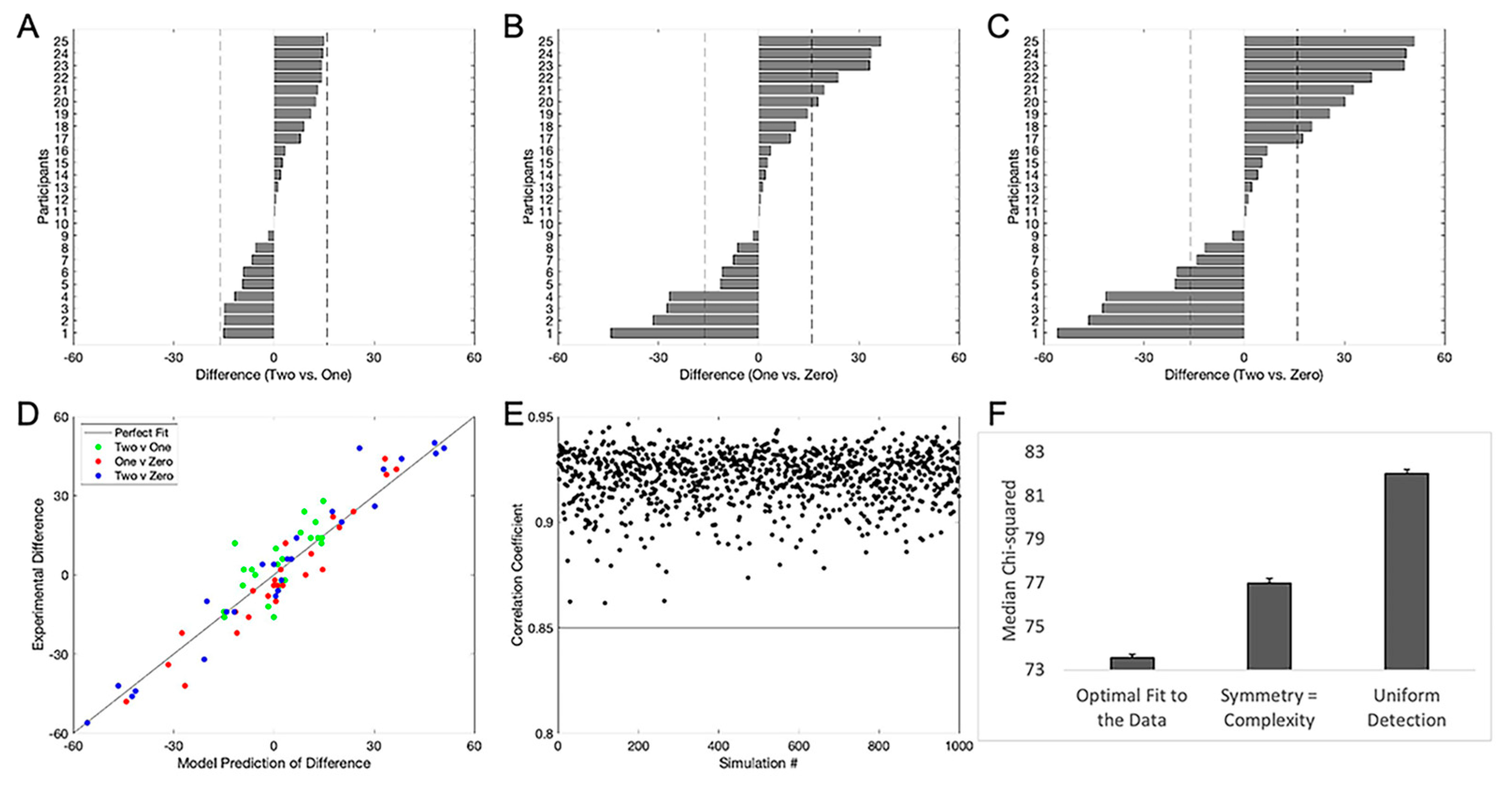
4.4.4. Results
4.4.5. Discussion
5. General Discussion
5.1. Time Required for the Detection of Multiple Axes of Symmetry
5.2. Why People like Multiple Axes of Symmetry
5.3. Do People Always Prefer Symmetry?
Supplementary Materials
Author Contributions
Funding
Institutional Review Board Statement
Informed Consent Statement
Data Availability Statement
Acknowledgments
Conflicts of Interest
References
- Rodríguez, I.; Gumbert, A.; Hempel de Ibarra, N.; Kunze, J.; Giurfa, M. Symmetry Is in the Eye of the ‘Beeholder’: Innate Preference for Bilateral Symmetry in Flower-Naïve Bumblebees. Naturwissenschaften 2004, 91, 374–377. [Google Scholar] [CrossRef] [PubMed]
- Treder, M.S. Behind the Looking-Glass: A Review on Human Symmetry Perception. Symmetry 2010, 2, 1510–1543. [Google Scholar] [CrossRef] [Green Version]
- Wenderoth, P. The Salience of Vertical Symmetry. Perception 1994, 23, 221–236. [Google Scholar] [CrossRef]
- Palmer, S.E.; Schloss, K.B.; Sammartino, J. Visual Aesthetics and Human Preference. Annu. Rev. Psychol. 2013, 64, 77–107. [Google Scholar] [CrossRef] [Green Version]
- Tinio, P.P.L.; Leder, H. Just How Stable Are Stable Aesthetic Features? Symmetry, Complexity, and the Jaws of Massive Familiarization. Acta Psychol. 2009, 130, 241–250. [Google Scholar] [CrossRef]
- Voloshinov, A.V. Symmetry as a Superprinciple of Science and Art. Leonardo 1996, 29, 109–113. [Google Scholar] [CrossRef]
- Aleem, H.; Correa-Herran, I.; Grzywacz, N.M. Inferring Master Painters’ Esthetic Biases from the Statistics of Portraits. Front. Hum. Neurosci. 2017, 11, 94. [Google Scholar] [CrossRef] [Green Version]
- Nucci, M.; Wagemans, J. Goodness of Regularity in Dot Patterns: Global Symmetry, Local Symmetry, and Their Interactions. Perception 2007, 36, 1305–1319. [Google Scholar] [CrossRef] [Green Version]
- Bichot, N.P.; Rossi, A.F.; Desimone, R. Parallel and Serial Neural Mechanisms for Visual Search in Macaque Area V4. Science 2005, 308, 529–534. [Google Scholar] [CrossRef] [Green Version]
- Shipp, S. The Brain Circuitry of Attention. Trends Cogn. Sci. 2004, 8, 223–230. [Google Scholar] [CrossRef]
- Sigman, M.; Dehaene, S. Brain Mechanisms of Serial and Parallel Processing during Dual-Task Performance. J. Neurosci. 2008, 28, 7585–7598. [Google Scholar] [CrossRef] [PubMed] [Green Version]
- Wagemans, J.; Van Gool, L.; D’ydewalle, G. Detection of Symmetry in Tachistoscopically Presented Dot Patterns: Effects of Multiple Axes and Skewing. Percept. Psychophys. 1991, 50, 413–427. [Google Scholar] [CrossRef] [PubMed] [Green Version]
- Sasaki, Y.; Vanduffel, W.; Knutsen, T.; Tyler, C.; Tootell, R. Symmetry Activates Extrastriate Visual Cortex in Human and Nonhuman Primates. Proc. Natl. Acad. Sci. USA 2005, 102, 3159–3163. [Google Scholar] [CrossRef] [PubMed]
- Tyler, C.W.; Baseler, H.A.; Kontsevich, L.L.; Likova, L.T.; Wade, A.R.; Wandell, B.A. Predominantly Extra-Retinotopic Cortical Response to Pattern Symmetry. Neuroimage 2005, 24, 306–314. [Google Scholar] [CrossRef]
- Cattaneo, Z. The Neural Basis of Mirror Symmetry Detection: A Review. J. Cogn. Psychol. 2017, 29, 259–268. [Google Scholar] [CrossRef]
- Chen, C.-C.; Kao, K.-L.C.; Tyler, C.W. Face Configuration Processing in the Human Brain: The Role of Symmetry. Cereb. Cortex 2007, 17, 1423–1432. [Google Scholar] [CrossRef] [Green Version]
- Saarinen, J.; Levi, D.M. Perception of Mirror Symmetry Reveals Long-Range Interactions between Orientation-Selective Cortical Filters. NeuroReport 2000, 11, 2133–2138. [Google Scholar]
- Tyler, C.W.; Hardage, L.; Miller, R.T. Multiple Mechanisms for the Detection of Mirror Symmetry. Spat. Vis. 1995, 9, 79–100. [Google Scholar]
- Tyler, C.W.; Hardage, L. Mirror Symmetry Detection: Predominance of Second-Order Pattern Processing throughout the Visual Field. In Human Symmetry Perception and Its Computational Analysis; Psychology Press: London, UK, 2002; ISBN 978-1-4106-0660-0. [Google Scholar]
- Desimone, R.; Gross, C.G. Visual areas in the temporal cortex of the macaque. Brain Res. 1979, 178, 363–380. [Google Scholar]
- Smith; Singh, K.D.; Williams, A.L.; Greenlee, M.W. Estimating Receptive Field Size from FMRI Data in Human Striate and Extrastriate Visual Cortex. Cereb. Cortex 2001, 11, 1182–1190. [Google Scholar] [CrossRef] [Green Version]
- Olivers, C.N.L.; van der Helm, P.A. Symmetry and Selective Attention: A Dissociation between Effortless Perception and Serial Search. Percept. Psychophys. 1998, 60, 1101–1116. [Google Scholar] [CrossRef] [PubMed] [Green Version]
- Pramod, R.T.; Arun, S.P. Symmetric objects become special in perception because of generic computations in neurons. Psychol. Sci. 2018, 29, 95–109. [Google Scholar] [PubMed]
- Tyler, C.W. The Symmetry Magnification Function Varies with Detection Task. J. Vis. 2001, 1, 7. [Google Scholar] [CrossRef] [PubMed]
- Dakin, S.C.; Herbert, A.M. The Spatial Region of Integration for Visual Symmetry Detection. Proc. R. Soc. Lond. Ser. B Biol. Sci. 1998, 265, 659–664. [Google Scholar] [CrossRef]
- Strasburger, H. Seven Myths on Crowding and Peripheral Vision. i-Perception 2020, 11, 2041669520913052. [Google Scholar] [CrossRef]
- Traquair, H.M. An Introduction to Clinical Perimetry; Henry Kimpton Publisher: London, UK, 1927. [Google Scholar]
- Aleem, H.; Pombo, M.; Correa-Herran, I.; Grzywacz, N.M. Is Beauty in the Eye of the Beholder or an Objective Truth? A Neuroscientific Answer. In Mobile Brain-Body Imaging and the Neuroscience of Art, Innovation and Creativity; Contreras-Vidal, J.L., Robleto, D., Cruz-Garza, J.G., Azorín, J.M., Nam, C.S., Eds.; Springer Series on Bio- and Neurosystems; Springer International Publishing: Cham, Switzerland, 2019; pp. 101–110. ISBN 978-3-030-24326-5. [Google Scholar]
- Reber, R.; Schwarz, N.; Winkielman, P. Processing Fluency and Aesthetic Pleasure: Is Beauty in the Perceiver’s Processing Experience? Pers. Soc. Psychol. Rev. 2004, 8, 364–382. [Google Scholar] [CrossRef] [Green Version]
- Cohen, J. Statistical Power Analysis for the Behavioral Sciences, 2nd ed.; L. Erlbaum Associates: Hillsdale, NJ, USA, 1988; ISBN 978-0-8058-0283-2. [Google Scholar]
- Champely, S. Pwr: Basic Functions for Power Analysis; R Package Version 1.3-0; 2020; Available online: https://cran.r-project.org/web/packages/pwr/.
- Correll, J.; Mellinger, C.; McClelland, G.H.; Judd, C.M. Avoid Cohen’s ‘Small’, ‘Medium’, and ‘Large’ for Power Analysis. Trends Cogn. Sci. 2020, 24, 200–207. [Google Scholar] [CrossRef]
- Peirce, J.; Gray, J.R.; Simpson, S.; MacAskill, M.; Höchenberger, R.; Sogo, H.; Kastman, E.; Lindeløv, J.K. PsychoPy2: Experiments in Behavior Made Easy. Behav. Res. 2019, 51, 195–203. [Google Scholar] [CrossRef] [Green Version]
- Hunter, J.D. Matplotlib: A 2D Graphics Environment. Comput. Sci. Eng. 2007, 9, 90–95. [Google Scholar] [CrossRef]
- R Core Team. R: A Language and Environment for Statistical Computing; R Foundation for Statistical Computing: Vienna, Austria, 2013; Available online: http://www.R-project.org/.
- Miller, D. Saccadic and Pursuit Systems: A Review. J. Pediatr. Ophthalmol. Strabismus 1968, 5, 39–43. [Google Scholar] [CrossRef]
- Carlson, T.A.; Hogendoorn, H.; Verstraten, F.A.J. The Speed of Visual Attention: What Time Is It? J. Vis. 2006, 6, 6–11. [Google Scholar] [CrossRef] [Green Version]
- Aleem, H.; Correa-Herran, I.; Grzywacz, N.M. A Theoretical Framework for How We Learn Aesthetic Values. Front. Hum. Neurosci. 2020, 14, 345. [Google Scholar] [CrossRef]
- Donderi, D.C. An Information Theory Analysis of Visual Complexity and Dissimilarity. Perception 2006, 35, 823–835. [Google Scholar] [CrossRef]
- Correa-Herran, I.; Aleem, H.; Grzywacz, N.M. Evolution of Neuroaesthetic Variables in Portrait Paintings throughout the Renaissance. Entropy 2020, 22, 146. [Google Scholar] [CrossRef] [PubMed] [Green Version]
- Güçlütürk, Y.; Jacobs, R.H.A.H.; van Lier, R. Liking versus Complexity: Decomposing the Inverted U-Curve. Front. Hum. Neurosci. 2016, 10, 112. [Google Scholar] [CrossRef] [PubMed]
- Tyler, C.W.; Chen, C.-C. Signal Detection Theory in the 2AFC Paradigm: Attention, Channel Uncertainty and Probability Summation. Vis. Res. 2000, 40, 3121–3144. [Google Scholar] [CrossRef] [Green Version]
- Andrews, L.C. Special Functions of Mathematics for Engineers; SPIE Press: Bellingham, WA, USA, 1998; ISBN 978-0-8194-2616-1. [Google Scholar]
- Pombo, M.; Brielmann, A.A.; Pelli, D.G. The Intrinsic Variance of Beauty Judgment. Atten. Percept. Psychophys. 2022, 85, 1355–1373. [Google Scholar]
- Rousseeuw, P.J.; Leroy, A.M. Robust Regression and Outlier Detection; Wiley Series in Probability and Mathematical Statistics; Wiley: New York, NY, USA, 1987; ISBN 978-0-471-85233-9. [Google Scholar]
- Nelder, J.A.; Mead, R. A Simplex Method for Function Minimization. Comput. J. 1965, 7, 308–313. [Google Scholar] [CrossRef]
- Wright, S.J. Coordinate Descent Algorithms. Math. Program. 2015, 151, 3–34. [Google Scholar] [CrossRef]
- Loaiza-Ganem, G.; Cunningham, J.P. The Continuous Bernoulli: Fixing a Pervasive Error in Variational Autoencoders. Adv. Neural Inf. Process. Syst. 2019, 32, 13287–13297. [Google Scholar]
- Bertamini, M.; Makin, A.; Pecchinenda, A. Testing Whether and When Abstract Symmetric Patterns Produce Affective Responses. PLoS ONE 2013, 8, e68403. [Google Scholar] [CrossRef]
- Makin, A.D.J.; Wright, D.; Rampone, G.; Palumbo, L.; Guest, M.; Sheehan, R.; Cleaver, H.; Bertamini, M. An Electrophysiological Index of Perceptual Goodness. Cereb. Cortex 2016, 26, 4416–4434. [Google Scholar] [CrossRef] [PubMed] [Green Version]
- Bertamini, M.; Rampone, G.; Makin, A.D.J.; Jessop, A. Symmetry Preference in Shapes, Faces, Flowers and Landscapes. PeerJ 2019, 7, e7078. [Google Scholar] [CrossRef] [PubMed] [Green Version]
- Pombo, M.; Pelli, D.G. Aesthetics: It’s Beautiful to Me. Curr. Biol. 2022, 32, R378–R379. [Google Scholar] [CrossRef] [PubMed]


Disclaimer/Publisher’s Note: The statements, opinions and data contained in all publications are solely those of the individual author(s) and contributor(s) and not of MDPI and/or the editor(s). MDPI and/or the editor(s) disclaim responsibility for any injury to people or property resulting from any ideas, methods, instructions or products referred to in the content. |
© 2023 by the authors. Licensee MDPI, Basel, Switzerland. This article is an open access article distributed under the terms and conditions of the Creative Commons Attribution (CC BY) license (https://creativecommons.org/licenses/by/4.0/).
Share and Cite
Pombo, M.; Aleem, H.; Grzywacz, N.M. Multiple Axes of Visual Symmetry: Detection and Aesthetic Preference. Symmetry 2023, 15, 1568. https://doi.org/10.3390/sym15081568
Pombo M, Aleem H, Grzywacz NM. Multiple Axes of Visual Symmetry: Detection and Aesthetic Preference. Symmetry. 2023; 15(8):1568. https://doi.org/10.3390/sym15081568
Chicago/Turabian StylePombo, Maria, Hassan Aleem, and Norberto M. Grzywacz. 2023. "Multiple Axes of Visual Symmetry: Detection and Aesthetic Preference" Symmetry 15, no. 8: 1568. https://doi.org/10.3390/sym15081568