Nonlinear Dynamic Modeling and Analysis for a Spur Gear System with Dynamic Meshing Parameters and Sliding Friction

Abstract

The performance of gear systems is closely related to the meshing parameters and sliding friction. However, the time-varying characteristics of meshing parameters caused by transverse vibration are usually not regarded and the sliding friction has always been ignored in previous studies. Therefore, the influence of the transverse vibration on meshing parameters and sliding friction have not been considered. In view of this, a nonlinear dynamic model for a spur gear system is proposed. The dynamic meshing parameters (pressure angle, backlash, etc.) and the effects of the variations of these parameters on the dynamic mesh force (DMF) and sliding friction are emphasized. The differential equations of motion are derived by the Lagrange method and solved by the Runge–Kutta method. Then, the input speed and friction coefficient are used as control parameters to compare the dynamic responses of the new and previous models. The results show that the meshing parameters and sliding friction are affected by transverse vibration, leading to distinctive nonlinear dynamic responses. This paper can provide a basis for further research and give a better understanding of system vibration control.

1. Introduction

Gear systems have the advantages of wide transmission power range, high efficiency, and accurate transmission ratio, and are widely used in aerospace, marine, and electric power fields as typical periodic symmetrical components [1]. The performance of the gear system directly affects the overall performance of mechanical equipment. Furthermore, the noise caused by vibration and shock during the operation of the gear system is one of the important components of mechanical equipment noise, which seriously influences comfort [2], and also affects the concealment of military equipment [3]. Therefore, it is of great significance to establish a proper dynamic model of gear systems and study the dynamic characteristics for engineering design, condition monitoring, and fault diagnosis.

For simplification, the influence of transverse vibration on gear meshing parameters is not considered in most of the existing gear system models, that is, the pressure angle, contact ratio, and backlash are all assumed to be constant [4,5,6,7,8]. In fact, the meshing parameters change due to the transverse vibration. With the urgent demand for lightweight design of gear systems in modern industry, especially in aerospace, flexible supporting structures such as thin hollow shafts and thin wall gearboxes have been widely used [9]. As the stiffness of the supporting structure decreases, the transverse vibration of the gear becomes obvious, and the prior model could not accurately predict the dynamic behavior. Scholars have recently begun to pay attention to this problem. Chen et al. [10] deduced the relationship between the backlash and the variation of center distance, and established a dynamic model considering the sliding friction, but they did not consider the change of the other mesh parameters under the influence of transverse vibration. Focusing on the time-varying pressure angle caused by the transverse vibration, Kim et al. [11] proposed a new spur gear system model, and on this basis studied the effects of stiffness and damping on the dynamic response of the system. Then, they [12] established a 15-degrees-of-freedom (DOFs) dynamic model with a planetary gear system as an object and analyzed the influence of bearing deformation on tooth deformation, pressure angle, and contact ratio between sun and star gears and between star and ring gears, as well as vibration displacement in different directions. Afterwards, Chen [13] extended the study to a helical gear system and investigated the effects of bearing radial and axial stiffness and mass eccentricity on dynamic response. Liu et al. [14] proposed a lateral–torsional–rocking coupled model of a gear system considering time-varying center distance and backlash, and analyzed the effects of different modification methods. Yi et al. [15] established a new nonlinear dynamic model of a spur gear considering the time-varying backlash, and the results showed that the calculated dynamic response was more realistic. Wang and Zhu [16] put forward a nonlinear dynamic model of a GTF gearbox with time-varying backlash, and investigated the dynamic characteristics from the time domain and frequency domain. Jedliński [17] focused on the influence of the off-line-of-action (OLOA) direction displacement on the distance between the meshing tooth surfaces along the line of action (LOA) and established a 12-DOFs analytical model. The results show that the influence of the OLOA displacement on the distance between the meshing tooth surfaces could not be neglected when the OLOA displacement was significant. Yang et al. [18] proposed a new method for calculating the mesh stiffness of a helical gear pair, which considered the time-varying backlash. Considering the effect of bearing clearance on the radial vibration of gears, Tian et al. [19] investigated the stability of the spur gear system in depth by selecting bifurcation parameters such as rotational speed and bearing clearance.

As one of the important excitation sources, the sliding friction between the tooth surface couples the motions of LOA and OLOA. The effect of sliding friction on the vibration and noise of the gear system cannot be ignored [20]. Singh and co-authors used Floquet theory [21], harmonic balance method [22], and the numerical method [23] to comprehensively study the sliding friction of a SDOF gear pair, and later extended this to multiple DOFs systems [24,25]. Ghosh and Chakraborty [26] studied the effects of friction coefficient, damping, and modification on the system stability of a six-DOF spur gear system. Zhou et al. [27] proposed a 16-DOFs coupling dynamic model of the gear rotor system, and studied the influence of the friction coefficient on the nonlinear characteristics of the system. They found that the system entered a chaotic state with the increase in friction coefficient within a certain range. Shi et al. [28] established a SDOF gear pair considering multi-state mesh and sliding friction and analyzed the effects of load coefficient, backlash, and comprehensive error on the system dynamic response. Afterwards, they carried out a study on the nonlinear dynamic characteristics of the system under random excitation [29]. Wang [30] built a bending-torsion-shaft-coupled model of the helical gear pair and investigated the influence of sliding friction through dynamic meshing force (DMF)/speed/displacement. Aiming at the loss-of-lubrication condition of helicopter gear transmission, Hu et al. [31] predicted the friction coefficient based on the computational inverse technique, and studied the nonlinear dynamic behavior of the system considering gyroscopic effect, thermal expansion, and wear under this working condition. The results show that although friction had little effect on the natural frequency, it had significant effect on nonlinear dynamic behavior. Luo et al. [32] established a dynamic model of the planetary gear sets to research the influence of the spalling defect on the dynamic performance when the sliding friction was considered. Jiang and Liu [33] paid attention to the axial friction caused by the axial mesh force in the helical gear system and pointed out that the oscillations of the dynamic responses become more significant incorporating the effects of coupled sliding friction.

In general, although scholars have conducted many studies on gear dynamics for different factors, few studies have simultaneously considered the influences of transverse vibration on the meshing parameters and sliding friction. The direction of sliding friction changes as the pressure angle changes, and the length of friction force arm is affected by the variation of center distance. The variations of meshing parameters and sliding friction affect the dynamic characteristics of the system and then change the transverse vibration response. This interaction should be taken into account in the study of gear dynamics. For this reason, a new dynamic model for a spur gear system with dynamic meshing parameters and sliding friction is proposed, and the dynamic characteristics of the system are analyzed on this basis.

The rest of this paper is organized as follows. In the next section, the dynamic meshing parameters affected by transverse vibration and the corresponding DMF and friction force are given and a six-DOFs nonlinear dynamic model for a spur gear system is developed with time-varying pressure angle, time-varying mesh stiffness (TVMS), dynamic backlash, and sliding friction. The equations of motion are strictly derived using the Lagrange method in Section 3. In Section 4, the dynamic responses of the new and previous models are compared, with the input speed and friction coefficient as the control parameters, respectively. In the last section, some brief conclusions are presented.

The main contributions of this paper are summarized as follows:

• We establish a new sliding friction model between the tooth surfaces considering the influence of the transverse vibration.
• Based on the sliding friction model, a new nonlinear dynamic model with dynamic meshing parameters and sliding friction is proposed.
• The effects of the input speed and friction coefficient on the dynamic response of the new model and the previous model are compared and analyzed.

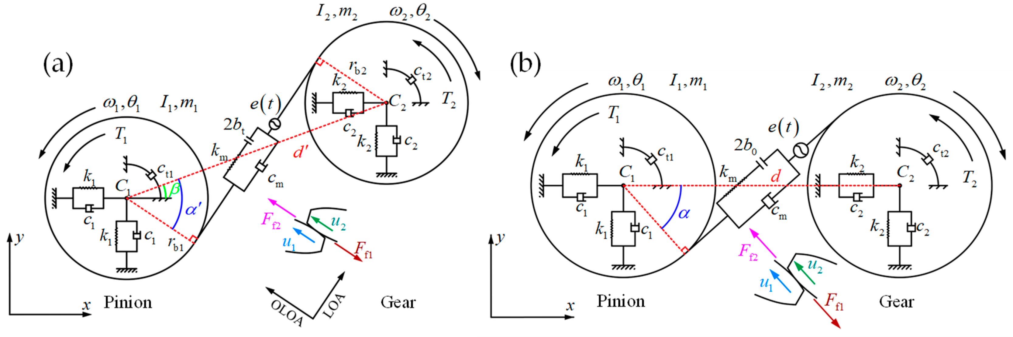
2. Dynamic Model for Spur Gear System

Figure 1a shows the dynamic model (new model) proposed in this paper, which considers the influence of transverse vibration on meshing parameters and sliding friction. Figure 1b shows the dynamic model (previous model) commonly used in previous studies that ignores the influence of transverse vibration, which assumes that the direction of the LOA remains constant during operation. As the main difference between the two models, the effects of transverse vibration on the system can be divided into two levels. The first includes the variations of the meshing parameters such as center distance, pressure angle, and backlash caused by transverse vibration. The second is the influence of these parameters on DMF and sliding friction. This paper focuses on these two levels to model the spur gear system with the influence of transverse vibration, which will be introduced in detail.

2.1. Dynamic Meshing Parameters under the Influence of Transverse Vibration

In Figure 1, subscript 1 and 2 represent the pinion (driving gear) and the gear (driven gear), respectively. The supporting structure of each gear is equivalent to two sets of spring-damping units, namely $k_{xi}$, $c_{xi}$, $k_{yi}$, and $c_{yi}\left(i=1,2\right)$, and the torsional damping unit $c_{\mathrm{t}i}$, which is used to explain the viscous loss caused by the bearings and shafts. This paper assumes that $c_{xi}=c_{yi}$ and $k_{xi}=k_{yi}$, so only $c_1$, $c_2$, $k_1$, and $k_2$ are indicated in Figure 1. $r_{\mathrm{b}i}$ is the radius of the base circle. $m_i$, $I_i$, and $T_i$ are the mass, moment of inertia, and external torque, respectively. ${\omega }_i$, ${\phi }_i$, and ${\theta }_i$ are, respectively, the angular speed, angular displacement, and small angular displacement resulting from torsional vibration. Figure 2 illustrates the generalized coordinates of the meshing gears, where the black dashed and blue solid lines separately represent the meshing gears before and after motion. The initial position of the rotation center of the gear is represented by $O_i$ and the position after the motion is denoted by $C_i$. $G_i$ is the mass center of the gear. Assuming that only the translational motion is considered, the coordinates of the gear can be given by the translation coordinates $x_i$, $y_i$ and the angular coordinate ${\phi }_i$. The angular displacements of the pinion and gear can be written as:

$${\phi }_1={\omega }_{1}t+{\theta }_1+{\phi }_{01}, {\phi }_2={\omega }_{2}t+{\theta }_2+{\phi }_{02}$$

(1)

where ${\phi }_{0i}$ is the initial angular displacement.

According to Figure 1a and Figure 2, when geometric eccentricity and material defects are ignored, the displacement vectors for the mass center of the pinion and gear at an arbitrary time can be expressed as:

$$\begin{array}{l}{r}_1=\left(x_1+{\epsilon }_1\cos {\phi }_1\right)i+\left(y_1+{\epsilon }_1\sin {\phi }_1\right)j\\ r_2=\left(x_2+{\epsilon }_2\cos {\phi }_2+d\right)i+\left(y_2-{\epsilon }_2\sin {\phi }_2\right)j \end{array}$$

(2)

where ${\epsilon }_i$ is the mass eccentricity, $i$ and $j$ are unit vectors along the $x$ and $y$ axes, respectively.

The time-varying pressure angle, that is, the acute angle sandwiched between the velocity direction at the pitch point and the LOA (Figure 1a), can be expressed as:

$${\alpha }^{\prime }={\cos }^{-1}\frac{r_{\mathrm{b}}{}_1+r_{\mathrm{b}2}}{d^{\prime }}$$

(3)

in which $d^{\prime }$ is the time-varying center distance, and the relationship between $d^{\prime }$ and the initial center distance $d$ is $d^{\prime }=\sqrt{{\left(x_2-x_1+d\right)}^2+{\left(y_2-y_1\right)}^2}$.

The contact ratio at any time is:

$$m_{\mathrm{p}}=\frac{\sqrt{r_{\mathrm{a}2}^2-r_{\mathrm{b}2}^2}+\sqrt{r_{\mathrm{a}2}^2-r_{\mathrm{b}2}^2}-d^{\prime }\sin {\alpha }^{\prime }}{p_{\mathrm{b}}}$$

(4)

where $r_{\mathrm{a}i}$ is the addendum radius of the gear, $p_{\mathrm{b}}$ is the base pitch, and $p_{\mathrm{b}}=\mathsf{\pi }m\cos \alpha$, in which $m$ is the module and $\alpha$ is the pressure angle of the reference circle.

It can be seen that for Equations (3) and (4) the gear translation caused by transverse vibration directly leads to the variation of center distance, which then affects the pressure angle and contact ratio, so that they are no longer constant.

Furthermore, the center distance alone is no longer sufficient to describe the relative position of the two gears as shown in Figure 1a and Figure 2. Therefore, it is necessary to define another position angle $\beta$, which is:

$$\beta ={\tan }^{-1}\frac{y_2-y_1}{x_2-x_1+d}$$

(5)

In Figure 1a, the contact between the tooth surfaces is equivalent to a spring-damping system along the LOA. The compression direction is defined as the positive direction, and the dynamic transmission error (DTE), i.e., the gear mesh deformation along the LOA, can be given as:

$$\delta =r_{\mathrm{b}1}{\theta }_1-r_{\mathrm{b}2}{\theta }_2+\left(x_1-x_2\right)\sin \left({\alpha }^{\prime }-\beta \right)+\left(y_1-y_2\right)\cos \left({\alpha }^{\prime }-\beta \right)-e(t)$$

(6)

where the static transmission error (STE) $e\left(t\right)=e_{\mathrm{a}}\sin \left(2\mathsf{\pi }{f}_{\mathrm{m}}t+{\varphi }_0\right)$, in which $e_{\mathrm{a}}$ is the amplitude of the STE, $f_{\mathrm{m}}$($=n_1{z}_1/60\left(n_2{z}_2/60\right)={\omega }_1{z}_1/2\mathsf{\pi }\left({\omega }_2{z}_2/2\mathsf{\pi }\right)$), is the meshing frequency and ${\varphi }_0$ is the initial phase.

$k_{\mathrm{m}}$ is the TVMS as shown in Figure 1. The analytical model proposed by Ma et al. [34] is applied to calculate the TVMS here, and the corresponding result is presented by the blue dotted line in Figure 3. The double-teeth meshing zone is from $\left(n+1-m_{\mathrm{p}}\right)T_{\mathrm{m}}$ to $n{T}_{\mathrm{m}}\left(n\ge 1 , n\in N+\right)$, and the single-tooth meshing zone is from $\left(n-1\right)T_{\mathrm{m}}$ to $\left(n+1-m_{\mathrm{p}}\right)T_{\mathrm{m}}$. $T_{\mathrm{m}}$ is the meshing period. Since the periodic composition of the TVMS is related to $m_{\mathrm{p}}$, the TVMS is also affected by transverse vibration. To simplify, the TVMS of the square wave form proposed by Kahraman and Singh [35] is adopted, as shown by the red line in Figure 3. The square wave is determined by $k_{\mathrm{h}}$ and $k_{\mathrm{l}}$, which are, respectively, the maximum and minimum value in a single mesh period. The time-varying mesh damping $c_{\mathrm{m}}$ can be expressed as $c_{\mathrm{m}}=2{\xi }_{\mathrm{m}}\sqrt{k_{\mathrm{m}}{I}_1{I}_2/\left(I_1{r}_{\mathrm{b}2}^2+I_2{r}_{\mathrm{b}1}^2\right)}$, in which ${\xi }_{\mathrm{m}}$ is the damping ratio.

Dynamic backlash $b_{\mathrm{t}}$ usually consists of constant backlash and time-varying backlash [14,15], namely:

$$2b_{\mathrm{t}}=2b_0+\Delta b$$

(7)

where $2b_0$ is the constant backlash, that is the initial or design backlash, which is generally guaranteed by the manufacturing tolerance or the installation center distance error. $\Delta b$ is the time-varying backlash, which is generally caused by the geometric eccentricity or the transverse vibration of the gear. This paper emphasizes the influence of transverse vibration. According to the involute principle, the time-varying backlash can be expressed as:

$$\Delta b=2\left(r_{\mathrm{b}1}+r_{\mathrm{b}2}\right)\left(\mathrm{inv}\left({\alpha }^{\prime }\right)-\mathrm{inv}\left(\alpha \right)\right)$$

(8)

where $\mathrm{inv}\left(x\right)$ is the involute function and $\mathrm{inv}\left(x\right)=\tan \left(x\right)-x$.

So far, the dynamic meshing parameters under the influence of transverse vibration have been determined.

2.2. DMF and Sliding Friction Force/Torque under the Influence of Transverse Vibration

Based on the viscoelastic theory, the DMF is composed of elastic force and damping force, which can be obtained by:

$$F_{\mathrm{m}}=k_{\mathrm{m}}{f}_1\left(\delta \right)+c_{\mathrm{m}}{f}_2\left(\dot{\delta }\right)$$

(9)

where $f_1\left(\delta \right)$ and $f_2\left(\dot{\delta }\right)$ are the displacement and velocity functions of the backlash, respectively. $f_1\left(\delta \right)$ and $f_2\left(\dot{\delta }\right)$ can be described as:

$$f_1\left(\delta \right)=\left\{\begin{array}{cc}\delta -b_{\mathrm{t}},& \delta >b_{\mathrm{t}}\\ 0,& \left|\delta \right|\le b_{\mathrm{t}}\\ \delta +b_{\mathrm{t}},& \delta <-b_{\mathrm{t}}\end{array}\right., f_2\left(\dot{\delta }\right)=\left\{\begin{array}{cc}\dot{\delta }-{\dot{b}}_{\mathrm{t}},& \delta >b_{\mathrm{t}}\\ 0,& \left|\delta \right|\le b_{\mathrm{t}}\\ \dot{\delta }+{\dot{b}}_{\mathrm{t}},& \delta <-b_{\mathrm{t}}\end{array}\right.$$

(10)

in which $\cdot$ represents the differential of time. The three conditions in Equation (10) correspond successively to non-impact state (drive-side tooth mesh), single-sided impact state (teeth separation), and double-sided impact state (back-side tooth mesh).

Although the sliding friction was involved in some prior studies, the influence of variations of the meshing parameters was not considered. Therefore, a new sliding friction model between contact tooth surfaces is proposed, in which the effect of variations of the meshing parameters is taken into account. Figure 4 shows the schematic diagram of sliding friction between the tooth surfaces. It should be noted that the reference coordinate system is rotated $\beta$ clockwise compared with Figure 1a. The direction of sliding friction in Figure 4 is consistent with that shown in Figure 1a. $N_1{N}_2$ is the theoretical LOA segment, $B_1$ and $B_2$ are the starting and ending points of the engagement, corresponding to the actual LOA segment. For the $j^{\mathrm{th}}$ meshing tooth pair, the sliding velocity between the pinion tooth surface and the gear tooth surface can be expressed as:

$$v_{\mathrm{s}j}\left(t\right)=u_{1j}\left(t\right)-u_{2j}\left(t\right)$$

(11)

where $j\in N+$ and $j\le \mathrm{ceil}\left(m_{\mathrm{p}}\right)$, $\mathrm{ceil}\left(x\right)$ is the integer function, $u_{ij}\left(t\right)$ is the instantaneous tangential velocity of the tooth surface at the meshing point. If the angular velocity fluctuations of the gear are neglected, $u_{ij}\left(t\right)$ can be written as:

$$u_{ij}\left(t\right)={\omega }_i{R}_{ij}\left(t\right)$$

(12)

In Equation (12), $R_{ij}\left(t\right)$ is the contact radius, and can be obtained by:

$$\begin{array}{l}{R}_{1j}\left(t\right)=\sqrt{r_{\mathrm{a}1}^2-r_{\mathrm{b}1}^2}+\mathrm{mod}(r_{\mathrm{b}1}{\omega }_{1}t,p_{\mathrm{b}})-p_{\mathrm{b}}j\\ R_{2j}\left(t\right)=\left(r_{\mathrm{b}1}+r_{\mathrm{b}2}\right)\tan {\alpha }^{\prime }-\sqrt{r_{\mathrm{a}1}^2-r_{\mathrm{b}1}^2}+p_{\mathrm{b}}j-\mathrm{mod}(r_{\mathrm{b}1}{\omega }_{1}t,p_{\mathrm{b}})\end{array}$$

(13)

where $\mathrm{mod}\left(\mathrm{num}1,\mathrm{num}2\right)$ is the remainder function. From Figure 4 and Equation (13), it can be seen that the direction and the force arm of the sliding friction are affected by the transverse vibration.

The direction of sliding friction will change at the pitch point. In order to reconcile the difference between the actual direction and the assumed direction, a sign function is introduced here, which can be written as:

$${\lambda }_j=\left\{\begin{array}{ll}1,\hfill & v_{\mathrm{s}j}>0\\ 0,\hfill & v_{\mathrm{s}j}=0\\ -1,\hfill & v_{\mathrm{s}j}<0\end{array}\right.$$

(14)

In addition, the load sharing ratio model proposed by Pedrero et al. [36] is employed to determine the DMF between different meshing tooth pairs. The DMF between the $j\mathrm{th}$ meshing tooth pair can be determined by:

$$F_{\mathrm{N}ij}=L_j\left(t\right)F_{\mathrm{m}}$$

(15)

where $L_j\left(t\right)$ is the load sharing ratio of the $j^{\mathrm{th}}$ meshing tooth pair.

According to the Coulomb friction law, the sliding friction force can be calculated by:

$$F_{\mathrm{f}ij}=L_j\left(t\right)F_{\mathrm{m}}$$

(16)

Subsequently, the sliding friction torque can be expressed as:

$$T_{\mathrm{f}ij}=F_{\mathrm{f}ij}{R}_{ij}\left(t\right)$$

(17)

Thus, the DMF and sliding friction force/torque under the influence of transverse vibration are deduced.

3. Derivation of Equations of Motion

The dynamic differential equations of the spur gear system are derived in this section. As shown in Figure 1a, the gear system has six DOFs. Hence, the generalized coordinate vector of the dynamic model is $q={[x_1 y_1 {\theta }_1 x_2 y_2 {\theta }_2]}^{\mathrm{T}}$. Accordingly, the system kinetic energy $T$, system potential energy $U$, and Rayleigh’s dissipation function $D$ for generalized coordinates can be expressed as:

$$\begin{array}{c}T=\left[m_1{\left(‖{\dot{r}}_1‖\right)}^2+m_2{\left(‖{\dot{r}}_2‖\right)}^2+I_1{\dot{\phi }}_1^2+I_2{\dot{\phi }}_2^2\right]/2\\ U=\left[k_1\left(x_1^2+y_1^2\right)+k_2\left(x_2^2+y_2^2\right)+k_{\mathrm{m}}{f}_1^2\left(\delta \right)\right]/2\\ D=\left[c_1\left({\dot{x}}_1^2+{\dot{y}}_1^2\right)+c_2\left({\dot{x}}_2^2+{\dot{y}}_2^2\right)+\left(c_{\mathrm{t}1}{\dot{\theta }}_1^2+c_{\mathrm{t}2}{\dot{\theta }}_2^2\right)+c_{\mathrm{m}}{f}_2^2\left(\delta \right)\right]/2\end{array}$$

(18)

The generalized force or torque subjected to the system can be given by:

$$\begin{array}{l}Q=\left\{{\displaystyle \sum _{j=1}^{n=\mathrm{ceil}\left(m_{\mathrm{p}}\right)}{F}_{\mathrm{f}1j}\cos \left({\alpha }^{\prime }-\beta \right)\hspace{1em}-{\displaystyle \sum _{j=1}^{n=\mathrm{ceil}\left(m_{\mathrm{p}}\right)}{F}_{\mathrm{f}1j}\sin \left({\alpha }^{\prime }-\beta \right)-m_{1}g}}\right.\\ \hspace{1em}{T}_1-{\displaystyle \sum _{j=1}^{n=\mathrm{ceil}\left(m_{\mathrm{p}}\right)}{F}_{\mathrm{f}1j}{R}_{1j}}\hspace{1em}-{\displaystyle \sum _{j=1}^{n=\mathrm{ceil}\left(m_{\mathrm{p}}\right)}{F}_{\mathrm{f}2j}\cos \left({\alpha }^{\prime }-\beta \right)}\\ \hspace{1em}{\left.{\displaystyle \sum _{j=1}^{n=\mathrm{ceil}\left(m_{\mathrm{p}}\right)}{F}_{\mathrm{f}2j}\sin \left({\alpha }^{\prime }-\beta \right)-m_{2}g}\hspace{1em}-T_2+{\displaystyle \sum _{j=1}^{n=\mathrm{ceil}\left(m_{\mathrm{p}}\right)}{F}_{\mathrm{f}2j}{R}_{2j}}\right\}}^{\mathrm{T}}\end{array}$$

(19)

The equations of motion of the spur gear system can be derived from Lagrange’s equation, which can be described as:

$$\frac{d}{dt}\left(\frac{\partial T}{\partial {\dot{q}}_i}\right)-\frac{\partial T}{\partial q_i}+\frac{\partial D}{\partial {\dot{q}}_i}+\frac{\partial U}{\partial q_i}=Q_i$$

(20)

where $q_i$ is the generalized coordinate of the system and $i=1,2,3,\dots ,n$. $n$ is the degree of system freedom.

Substituting Equations (18) and (19) into Equation (20), the equations of motion of the spur gear system considering the influence of transverse vibration on meshing interface can be obtained as:

$$\begin{array}{l}{m}_1\left({\ddot{x}}_1-{\epsilon }_1{\ddot{\theta }}_1\sin {\phi }_1-{\epsilon }_1{\dot{\phi }}_1^2\cos {\phi }_1\right)+c_1{\dot{x}}_1+c_{\mathrm{m}}{f}_2\left(\delta \right)f_{2,{\dot{x}}_1}+k_1{x}_1+k_{\mathrm{m}}{f}_1\left(\delta \right)f_{1,x_1}={\displaystyle \sum _{j=1}^{n=\mathrm{ceil}\left(m_{\mathrm{p}}\right)}{F}_{\mathrm{f}1j}\cos \left({\alpha }^{\prime }-\beta \right)}\\ m_1\left({\ddot{y}}_1+{\epsilon }_1{\ddot{\theta }}_1\cos {\phi }_1-{\epsilon }_1{\dot{\phi }}_1^2\sin {\phi }_1\right)+c_1{\dot{y}}_1+c_{\mathrm{m}}{f}_2\left(\delta \right)f_{2,{\dot{y}}_1}+k_1{y}_1+k_{\mathrm{m}}{f}_1\left(\delta \right)f_{1,y_1}=-m_{1}g-{\displaystyle \sum _{j=1}^{n=\mathrm{ceil}\left(m_{\mathrm{p}}\right)}{F}_{\mathrm{f}1j}\sin \left({\alpha }^{\prime }-\beta \right)}\\ \left(I_1+m_1{\epsilon }_1^2\right){\ddot{\theta }}_1-m_1{\epsilon }_1\left({\ddot{x}}_1\sin {\phi }_1-{\ddot{y}}_1\cos {\phi }_1\right)+c_{\mathrm{t}1}{\dot{\phi }}_1+c_{\mathrm{m}}{f}_2\left(\delta \right)f_{2,{\dot{\theta }}_1}+k_{\mathrm{m}}{f}_1\left(\delta \right)f_{1,{\theta }_1}=T_1-{\displaystyle \sum _{j=1}^{n=\mathrm{ceil}\left(m_{\mathrm{p}}\right)}{F}_{\mathrm{f}1j}{R}_{1j}}\\ m_2\left({\ddot{x}}_2-{\epsilon }_2{\ddot{\theta }}_2\sin {\phi }_2-{\epsilon }_2{\dot{\phi }}_2^2\cos {\phi }_2\right)+c_2{\dot{x}}_2+c_{\mathrm{m}}{f}_2\left(\delta \right)f_{2,{\dot{x}}_2}+k_2{x}_2+k_{\mathrm{m}}{f}_1\left(\delta \right)f_{1,x_2}=-{\displaystyle \sum _{j=1}^{n=\mathrm{ceil}\left(m_{\mathrm{p}}\right)}{F}_{\mathrm{f}2j}\cos \left({\alpha }^{\prime }-\beta \right)}\\ m_2\left({\ddot{y}}_2-{\epsilon }_2{\ddot{\theta }}_2\cos {\phi }_2+{\epsilon }_2{\dot{\phi }}_2^2\sin {\phi }_2\right)+c_2{\dot{y}}_2+c_{\mathrm{m}}{f}_2\left(\delta \right)f_{2,{\dot{y}}_2}+k_2{y}_2+k_{\mathrm{m}}{f}_1\left(\delta \right){\delta }_{,y_2}=-m_{2}g+{\displaystyle \sum _{j=1}^{n=\mathrm{ceil}\left(m_{\mathrm{p}}\right)}{F}_{\mathrm{f}2j}\sin \left({\alpha }^{\prime }-\beta \right)}\\ \left(I_2+m_2{\epsilon }_2^2\right){\ddot{\theta }}_2-m_2{\epsilon }_2\left({\ddot{x}}_2\sin {\phi }_2+{\ddot{y}}_2\cos {\phi }_2\right)+c_{\mathrm{t}2}{\dot{\phi }}_2+c_{\mathrm{m}}{f}_2\left(\delta \right)f_{2,{\dot{\theta }}_2}+k_{\mathrm{m}}{f}_1\left(\delta \right)f_{1,{\theta }_2}=-T_2+{\displaystyle \sum _{j=1}^{n=\mathrm{ceil}\left(m_{\mathrm{p}}\right)}{F}_{\mathrm{f}2j}{R}_{2j}}\end{array}$$

(21)

where the comma in the subscript represents the partial differentiation, e.g., $f_{,x_1}=\partial f/\partial x_1$ and $f_{,{\dot{x}}_1}=\partial f/\partial {\dot{x}}_1$. The expressions for the remaining variables are as follows:

$$f_{1,x_i}=\left\{\begin{array}{cc}{\delta }_{,x_i}-b_{\mathrm{t},x_i},& \delta >b_{\mathrm{t}}\hfill \\ 0,& \left|\delta \right|\le b_{\mathrm{t}}\hfill \\ {\delta }_{,x_i}+b_{\mathrm{t},x_i},& \delta <-b_{\mathrm{t}}\hfill \end{array}\right.\hspace{1em}\left(i=1,2\right)$$

(22)

$$f_{1,y_i}=\left\{\begin{array}{cc}{\delta }_{,y_i}-b_{\mathrm{t},y_i},& \delta >b_{\mathrm{t}}\hfill \\ 0,& \left|\delta \right|\le b_{\mathrm{t}}\hfill \\ {\delta }_{,y_i}+b_{\mathrm{t},y_i},& \delta <-b_{\mathrm{t}}\hfill \end{array}\right.\hspace{1em}\left(i=1,2\right)$$

(23)

$$f_{1,{\theta }_1}=\left\{\begin{array}{cc}{r}_{\mathrm{b}1}-b_{\mathrm{t},{\theta }_1},& \delta >b_{\mathrm{t}}\hfill \\ 0,& \left|\delta \right|\le b_{\mathrm{t}}\hfill \\ r_{\mathrm{b}1}+b_{\mathrm{t},{\theta }_1},& \delta <-b_{\mathrm{t}}\hfill \end{array}\right.$$

(24)

$$f_{1,{\theta }_2}=\left\{\begin{array}{cc}-r_{\mathrm{b}2}-b_{\mathrm{t},{\theta }_2},& \delta >b_{\mathrm{t}}\hfill \\ 0,& \left|\delta \right|\le b_{\mathrm{t}}\hfill \\ -r_{\mathrm{b}1}+b_{\mathrm{t},{\theta }_2},& \delta <-b_{\mathrm{t}}\hfill \end{array}\right.$$

(25)

$$b_{\mathrm{t},x_i}=\left(r_{\mathrm{b}1}+r_{\mathrm{b}2}\right){{\alpha }^{\prime }}_{,x_i}{\tan }^2{\alpha }^{\prime }$$

(26)

$$b_{\mathrm{t},y_i}=\left(r_{\mathrm{b}1}+r_{\mathrm{b}2}\right){{\alpha }^{\prime }}_{,y_i}{\tan }^2{\alpha }^{\prime }$$

(27)

$$b_{\mathrm{t},{\theta }_i}=0$$

(28)

$$f_{2,{\dot{x}}_i}=f_{1,x_i},\hspace{1em}{f}_{2,{\dot{y}}_i}=f_{1,y_i},\hspace{1em}{f}_{2,{\dot{\theta }}_i}=f_{1,{\theta }_i}$$

(29)

$$\dot{\delta }={\dot{x}}_1{\delta }_{,x_1}+{\dot{y}}_1{\delta }_{,y_1}+{\dot{\theta }}_1{\delta }_{,{\theta }_1}+{\dot{x}}_2{\delta }_{,x_2}+{\dot{y}}_2{\delta }_{,y_2}+{\dot{\theta }}_2{\delta }_{,{\theta }_2}-\dot{e}(t)$$

(30)

$${\dot{b}}_{\mathrm{t}}=\left[\left(r_{\mathrm{b}1}+r_{\mathrm{b}2}\right){\tan }^2{\alpha }^{\prime }\right]\left({\dot{x}}_1{{\alpha }^{\prime }}_{,x_1}+{\dot{y}}_1{{\alpha }^{\prime }}_{,y_1}+{\dot{x}}_2{{\alpha }^{\prime }}_{,x_2}+{\dot{y}}_2{{\alpha }^{\prime }}_{,y_2}\right)$$

(31)

$${\delta }_{,x_1}=\sin \left({\alpha }^{\prime }-\beta \right)+\left[\left(x_1-x_2\right)\cos \left({\alpha }^{\prime }-\beta \right)-\left(y_1-y_2\right)\sin \left({\alpha }^{\prime }-\beta \right)\right]\left({{\alpha }^{\prime }}_{,x_1}-{\beta }_{,x_1}\right)$$

(32)

$${\delta }_{,y_1}=\cos \left({\alpha }^{\prime }-\beta \right)+\left[\left(x_1-x_2\right)\cos \left({\alpha }^{\prime }-\beta \right)-\left(y_1-y_2\right)\sin \left({\alpha }^{\prime }-\beta \right)\right]\left({{\alpha }^{\prime }}_{,y_1}-{\beta }_{,y_1}\right)$$

(33)

$${\delta }_{,{\theta }_1}=r_{\mathrm{b}1}$$

(34)

$${\delta }_{,x_2}=-\sin \left({\alpha }^{\prime }-\beta \right)+\left[\left(x_1-x_2\right)\cos \left({\alpha }^{\prime }-\beta \right)-\left(y_1-y_2\right)\sin \left({\alpha }^{\prime }-\beta \right)\right]\left({{\alpha }^{\prime }}_{,x_2}-{\beta }_{,x_2}\right)$$

(35)

$${\delta }_{,y_2}=-\cos \left({\alpha }^{\prime }-\beta \right)+\left[\left(x_1-x_2\right)\cos \left({\alpha }^{\prime }-\beta \right)-\left(y_1-y_2\right)\sin \left({\alpha }^{\prime }-\beta \right)\right]\left({{\alpha }^{\prime }}_{,y_2}-{\beta }_{,y_2}\right)$$

(36)

$${\delta }_{,{\theta }_2}=-r_{\mathrm{b}2}$$

(37)

in which:

$${{\alpha }^{\prime }}_{,x_1}=-{{\alpha }^{\prime }}_{,x_2}=-\frac{\left(x_2-x_1+d\right)\left(r_{\mathrm{b}1}+r_{\mathrm{b}2}\right)}{\left[{\left(x_2-x_1+d\right)}^2+{\left(y_2-y_1\right)}^2\right]\sqrt{{\left(x_2-x_1+d\right)}^2+{\left(y_2-y_1\right)}^2-{\left(r_{\mathrm{b}1}+r_{\mathrm{b}2}\right)}^2}}$$

(38)

$${{\alpha }^{\prime }}_{,y_1}=-{{\alpha }^{\prime }}_{,y_2}=-\frac{\left(y_2-y_1\right)\left(r_{\mathrm{b}1}+r_{\mathrm{b}2}\right)}{\left[{\left(x_2-x_1+d\right)}^2+{\left(y_2-y_1\right)}^2\right]\sqrt{{\left(x_2-x_1+d\right)}^2+{\left(y_2-y_1\right)}^2-{\left(r_{\mathrm{b}1}+r_{\mathrm{b}2}\right)}^2}}$$

(39)

$${\beta }_{,x_1}=-{\beta }_{,x_2}=\frac{y_2-y_1}{{\left(x_2-x_1+d\right)}^2+{\left(y_2-y_1\right)}^2}$$

(40)

$${\beta }_{,y_1}=-{\beta }_{,y_2}=-\frac{x_2-x_1+d}{{\left(x_2-x_1+d\right)}^2+{\left(y_2-y_1\right)}^2}$$

(41)

It can be seen from Equation (21) that the equations of motion of the system are nonlinear and coupled with each other. This also shows that the transverse vibration will affect the meshing parameters and change the DMF and sliding friction, etc. These changes will in turn affect the dynamic characteristics of the system, and then affect the time-varying characteristics of the meshing parameters and sliding friction.

When the influence of transverse vibration is ignored, the model (Figure 1b) commonly used in previous studies can be obtained by replacing ${\alpha }^{\prime }$ with $\alpha$, $b_{\mathrm{t}}$ with $b_0$, and setting $\beta =0$. The detailed description of the previous model refers to the work of He [20] or Chen et al. [10].

4. Comparison and Discussion of Dynamic Response

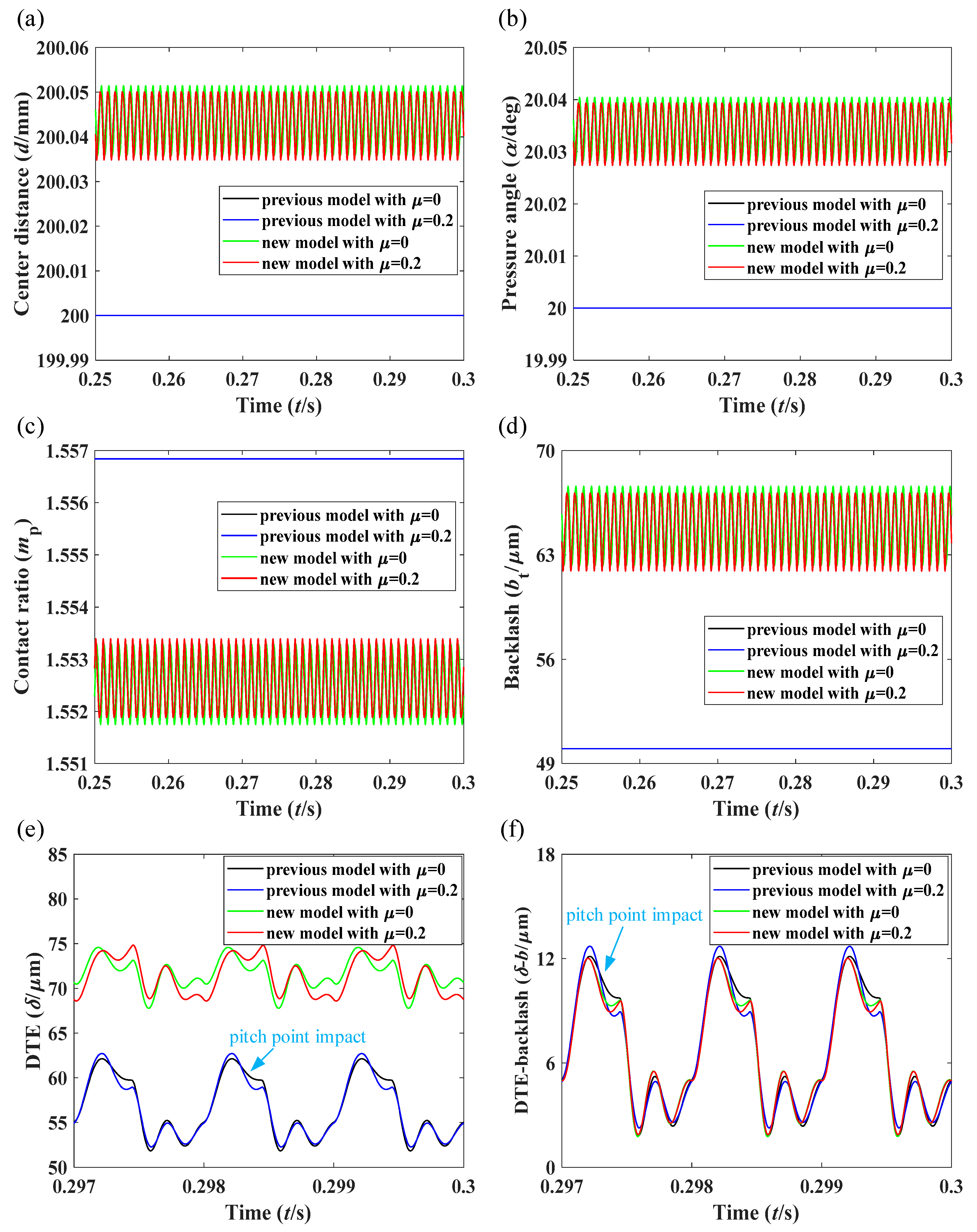
4.1. System Parameters and Model Validation

Geometrical and physical parameters of the spur gear system are listed in

Table 1. Geometrical and physical parameters of spur gear system.

Parameters	Symbols	Values
Module/(mm)	$m$	10
Number of teeth	$z_1$$/z_2$	20/20
Pressure angle of reference circle/(deg)	$\alpha$	20
Addendum coefficient	$h^{\ast }$	1
Tip clearance coefficient	$c^{\ast }$	0.25
Face width/(mm)	$L$	30
Gear mass/(kg)	$m_1$$/m_2$	6.57/6.57
Moment of inertia/(kg·m2)	$I_1$$/I_2$	0.0365/0.0365
Designed contact ratio	$m_{\mathrm{p}}$	1.5568
Equivalent shaft-bearing stiffness/(N/m)	$k_1$$/k_2$	1 × 108
Equivalent shaft-bearing damping/(N·s/m)	$c_1$$/c_2$	512.64/512.64
Torsional damping/(N·s/m)	$c_{\mathrm{t}1}$$/c_{\mathrm{t}2}$	143.29/143.29

. Gravity and mass eccentricity are neglected in the following study. Due to the strong nonlinearity and time variation, MATLAB ode15s, which is suitable for solving stiff problems, is used to simulate [37].

For validation purposes, the method in Ref. [15] is used here, that is, some key dynamic responses of the new and previous models are compared. The same parameters are utilized in this section. Furthermore, the input and output torque are $300 \mathrm{N}\cdot \mathrm{m}$. Figure 5 shows the time-domain responses of center distance, pressure angle, contact ratio, backlash, and DTE and the difference of DTE and backlash under different friction coefficients.

As shown in Figure 5a–d, the meshing parameters (i.e., center distance, pressure angle, contact ratio, and backlash) of the previous model remain unchanged. However, these meshing parameters of the new model display time-varying characteristics due to the consideration of the influence of transverse vibration. Moreover, the change of friction coefficient has effects on the meshing parameters. The center distance, pressure angle and backlash of the new model are greater than the theoretical value or the design value, and the contact ratio is less than the theoretical value. In Figure 5e, the pitch point impact caused by the change of sliding friction direction can be clearly seen in the DTE curves of the previous model. However, the pitch point impact of the new model is not obvious. This is because the backlash of the previous model is constant, and the influence of sliding friction is directly reflected in the DTE response, thus affecting the DMF. For the new model, sliding friction not only affects the DTE but also affects the backlash. With reference to Equations (7), (8) and (21), the influence of sliding friction on DMF depends on the difference between the DTE and the backlash. For better illustration, Figure 5f illustrates the response curve of the difference between DTE and backlash. Compared with Figure 5e, the shape of the difference curve of the previous model is the same as the DTE due to the constant backlash, with translation. The difference curve of the new model changes obviously, similar to the difference curve of the previous model, and the pitch point impact can also be observed clearly.

It can be seen that the transverse vibration has an obvious influence on the meshing parameters and sliding friction, which affects the dynamic characteristics of the system. Therefore, compared with the previous model, the new model can to some extent provide a more realistic response prediction. Next, this paper will further study the influence of input speed and sliding friction coefficient on the system dynamic response.

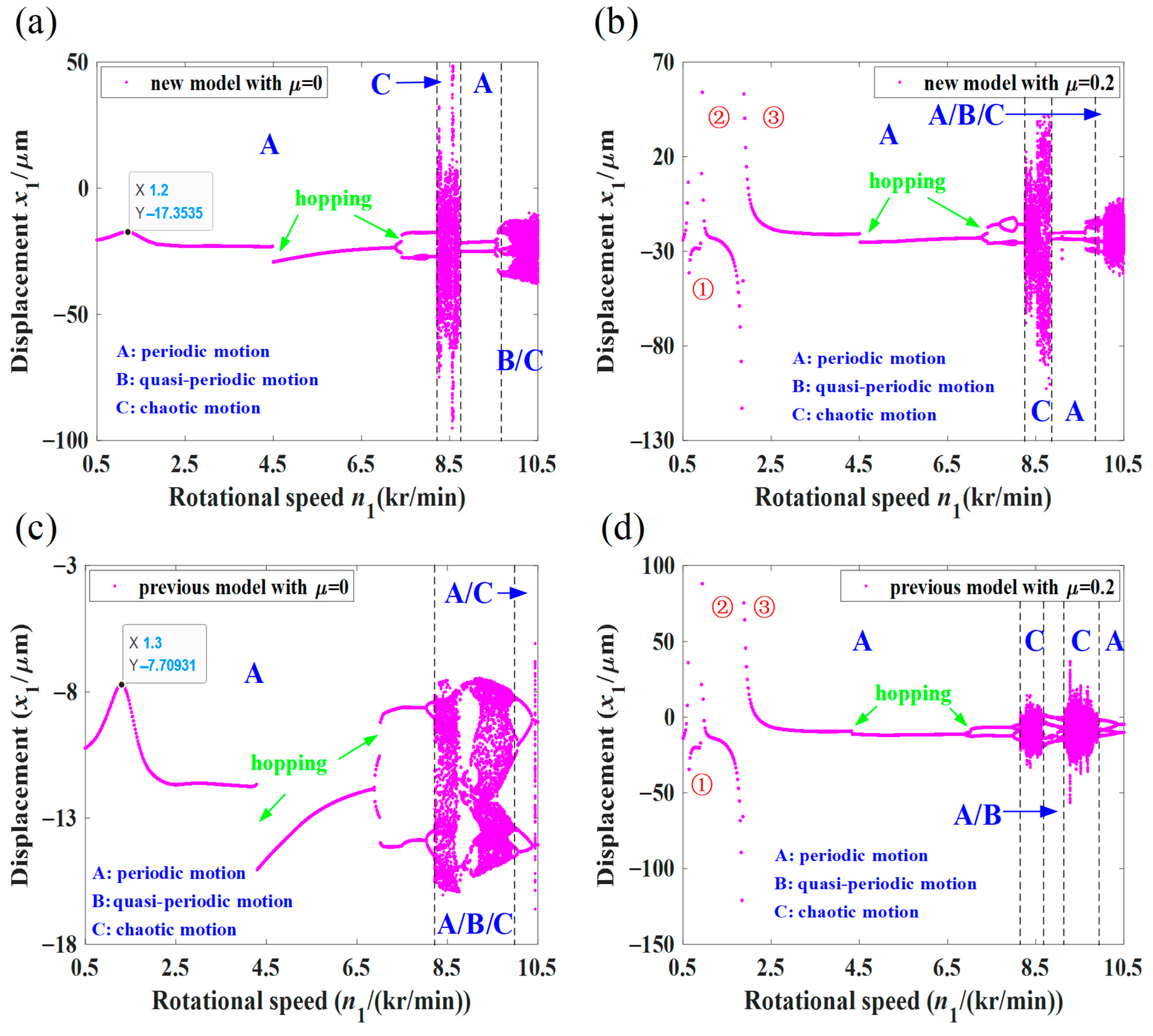
4.2. Effect of the Input Speed on System Dynamic Response

The gear system exhibits different dynamic behavior under different input speed. In this section, the input speed is used as the control parameter to study the dynamic behaviors of the system.

4.2.1. Chaotic Response of the System with $\mu =0$ and $\mu =0.2$

The global characteristics of the new and previous models are compared via bifurcation diagrams with respect to the input speed $n_1$, as shown in Figure 6. In order to further illustrate the necessity of considering the sliding friction, two cases $\mu =0$ and $\mu =0.2$ are considered. Figure 6 indicates that the steady-state motion of the system presents complex bifurcation characteristics with the variation of the input speed in both new and previous models. It can be observed that the two models have obvious differences in predicting the global characteristics.

When $\mu =0$, both two models perform periodic motion in the range of $\left[500, 8200\right]\mathrm{r}/\min$ as shown in Figure 6a,c. With the increase in input speed, the new model undergoes chaotic motion in the range of $\left(8200, 8720\right]\mathrm{r}/\min$ and periodic motion in the range of $\left(8720, 9620\right]\mathrm{r}/\min$. In the range of $\left(9620, \mathrm{10,500}\right]\mathrm{r}/\min$, the motion of the new model is mainly chaotic, but there also appears quasi-periodic motion. The previous model mainly experiences chaotic motion in the range of $\left(8220, 9960\right]\mathrm{r}/\min$, turning into periodic motion in the regions of $\left(9960, \mathrm{10,500}\right]\mathrm{r}/\min$. The new model resonates at $1200 \mathrm{r}/\min$, earlier than $1300 \mathrm{r}/\min$ in the previous model. Comparing Figure 6b,d, the new model and the previous model perform periodic motion in the regions of $\left[500, 8240\right]\mathrm{r}/\min$ and $\left[500, 8140\right]\mathrm{r}/\min$, respectively. In the ranges of $\left(8240, 8820\right]\mathrm{r}/\min$ and $\left(8820, 9860\right]\mathrm{r}/\min$, the new model undergoes chaotic and periodic motion, respectively. Then, the new model carries out several bifurcations of quasi-periodic motion and chaotic motion at $9880 \mathrm{r}/\min$, $\mathrm{10,040} \mathrm{r}/\min$, and $\mathrm{10,060} \mathrm{r}/\min$, and finally enters chaos. The previous model performs chaotic motion in the regions of $\left(8140, 8640\right]\mathrm{r}/\min$ and $\left(9140, 9900\right]\mathrm{r}/\min$, and mainly undergoes periodic and quasi-periodic motions in the range of $\left(8640, 9140\right]\mathrm{r}/\min$. The previous model returns to periodic motion at $n_1>9900 \mathrm{r}/\min$. It can be seen in Figure 6b,d that both models have three resonance peaks at $620 \mathrm{r}/\min$, $940 \mathrm{r}/\min$, and $1880 \mathrm{r}/\min$, as indicated by the red circle numbers. Compared with the case of $\mu =0$, the occurrence of these resonance points is caused by sliding friction. The region $1880 \mathrm{r}/\min$ corresponds to the torsional natural frequency of the system (620 Hz), $940 \mathrm{r}/\min$ and $620 \mathrm{r}/\min$ correspond to the first- and second-order super-harmonic resonances, respectively. These resonance peaks greatly affect the observation of the resonance peaks at $1200 \mathrm{r}/\min$ and $1300 \mathrm{r}/\min$. Furthermore, the sliding friction has a significant effect on the hopping and bifurcation points of the two models. Considering the complex operation conditions of the gear system, the rotational speed may fluctuate slightly. In order to avoid the instability caused by the system rotational speed falling near the corresponding speed of the bifurcation point, it is necessary to consider the sliding friction in order to predict more accurately. Consequently, the subsequent part of this section gives only the result comparisons for $\mu =0.2$.

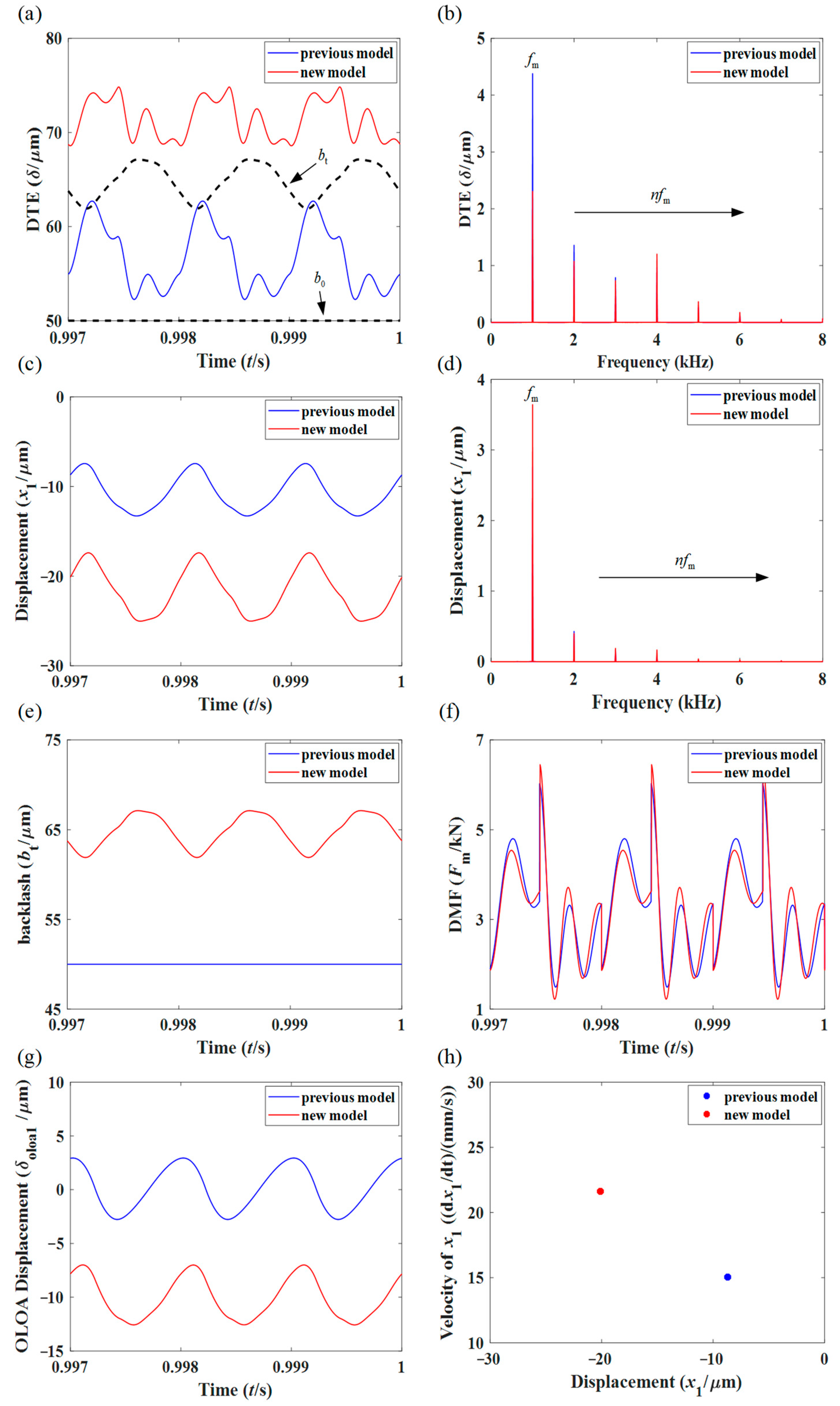
4.2.2. Comparison of Dynamic Responses at Different Input Speed with $\mu =0.2$

Based on the bifurcation diagram, $n_1=3000 \mathrm{r}/\min$, $7000 \mathrm{r}/\min$, $9500 \mathrm{r}/\min$, and $10,400 \mathrm{r}/\min$ are selected as examples to analyze the dynamic response of the system.

Figure 7 shows the comparison of dynamic responses of the new and previous models at $n_1=3000 \mathrm{r}/\min$. From Figure 7a,b, the DTE amplitude of the new model is larger than that of the previous model, and the amplitude difference of DTE between the two models is mainly concentrated in $f_{\mathrm{m}}$, $2f_{\mathrm{m}}$ and $4f_{\mathrm{m}}$. In Figure 7c, the mean value of vibration displacement $x_1$ of the new model is larger and the fluctuation of the new model is enhanced. The frequency-domain responses of $x_1$ in both models consist of the meshing frequency multiplication components ($n{f}_{\mathrm{m}}$), and the amplitude difference of $f_{\mathrm{m}}$ is the most obvious, as shown in Figure 7d. As shown in Figure 7e, the backlash of the previous model is constant and the relative relationship between the DTE and backlash is intuitive. Therefore, it is generally not necessary to draw the backlash curve along with the DTE curve when judging the meshing state. However, the backlash of the new model is time-variable. It may not be so intuitive to determine the relative relationship between the two time variables ($\delta$ and $b_{\mathrm{t}}$), and the response curve of the backlash is required to assist, as indicated by the black dashed line in Figure 7a (the backlash of the previous model is also drawn). It can be seen that the DTEs of the two models are always greater than the backlash, so they are each in a non-impact state, and $F_{\mathrm{m}}$ (Figure 7f) is always larger than 0. Although the DTE of the new model is much higher than that of the previous model, the difference between the DMF in the two models is not evident. This is because the backlash also becomes larger after considering the influence of transverse vibration. Figure 5f can also give a certain explanation, that is, the difference curves of the DTE and backlash of the two models are similar, and similar DMF results are obtained. As shown in Figure 7g, the mean value of the OLOA displacement of the previous model (${\delta }_{\mathrm{oloa}1}=x_1\cos \alpha -y_1\sin \alpha$) is far less than that of the new model (${\delta }_{\mathrm{oloa}1}=x_1\cos \left({\alpha }^{\prime }-\beta \right)-y_1\sin \left({\alpha }^{\prime }-\beta \right)$). The difference in DMF between the two models is not obvious, which means that the difference in sliding friction force is also not obvious. Therefore, the difference between ${\delta }_{\mathrm{oloa}1}$ in the two models is obviously due to the consideration of the influence of the transverse vibration in the new model. The Poincaré map for the two models, which reveals that both models experience period-1 motion, is shown in Figure 7h.

Figure 8 performs the same comparison as Figure 7 at $n_1=7000 \mathrm{r}/\min$. From Figure 8a,c, the DTE amplitude, the mean value, and the fluctuation of $x_1$ of the new model are still larger than those of the previous model. Compared with the new model, in addition to the amplitude difference at $f_{\mathrm{m}}$, $2f_{\mathrm{m}}$, and $3f_{\mathrm{m}}$, the frequency components of $n{f}_{\mathrm{m}}/2$ ($n$ is an odd number) also appear in the DTE and $x_1$ frequency-domain responses of the previous model, as shown in Figure 8b,d. It can be seen from Figure 8e that the backlash of the new model is still larger than the initial one. Compared with Figure 7e, the amplitude change of the dynamic backlash is not obvious with the increase in input speed. Comparing the real and dashed lines in Figure 8a, it can be found that $\delta <b_{\mathrm{t}}\left(b_0\right)$ occurs in both models, but $\delta$ is always greater than $-b_{\mathrm{t}}\left(b_0\right)$, so both models are in a single-sided impact state. The situation of $F_{\mathrm{m}}=0$ appears as illustrated in Figure 8f, and the phenomenon of teeth separation occurs periodically. When the meshing state is switched from drive-side tooth mesh to teeth separation, the DMF first decreases to 0 and then increases in the reverse direction, resulting in tooth surface impact as shown in the magnified figure in Figure 8f. The transition process of the DMF can be described as $F_{\mathrm{m}}>0\to F_{\mathrm{m}}=0\to F_{\mathrm{m}}<0\to F_{\mathrm{m}}=0$. Afterwards, the gear system enters teeth separation and the DMF is equal to 0 until the gear tooth meshes again. Both the mean value and amplitude of ${\delta }_{\mathrm{oloa}1}$ in the new model are greater than those of the previous model, as shown in Figure 8g. It can be seen from the time-domain response and the Poincaré map (Figure 8h) that the previous model undergoes period-2 motion, while the new model still experiences period-1 motion.

Figure 9 illustrates the same comparison at $n_1=9500 \mathrm{r}/\min$. The complex time-domain response, the continuous spectrum in the frequency-domain response, and the Poincaré map show that the previous model has entered chaos. The period of the DTE and $x_1$ responses, the presence of $n{f}_{\mathrm{m}}/2$ ($n$ is an odd number) components, and the Poincaré map indicate that the new model experiences period-2 motion. The new model is still in a single-sided impact state. As for the previous model, $\delta <-b_0$ occurs and it is in a double-sided impact state. As shown in Figure 9e, the dynamic backlash is still higher than the initial backlash. Compared with Figure 8f, the previous model in Figure 9f not only converts the drive-side tooth mesh into teeth separation as shown in magnified figure A (in Figure 9f), but also changes from teeth separation to back-side tooth mesh as shown in magnified figure B (in Figure 9f). As the system moves from teeth separation to back-side tooth mesh, the DMF changes from $F_{\mathrm{m}}=0\to F_{\mathrm{m}}<0\to F_{\mathrm{m}}=0\to F_{\mathrm{m}}>0\to F_{\mathrm{m}}=0$, resulting in tooth surface impact. The DMF transition process of the new model is similar to that shown in Figure 8f.

When $n_1=\mathrm{10,400} \mathrm{r}/\min$, the comparison of dynamic responses of the two models is shown in Figure 10. It can be seen that the previous model undergoes period-2 motion, and obvious $0.5f_{\mathrm{m}}$ and $f_{\mathrm{m}}$ components appear in the frequency-domain responses of DTE and $x_1$. The new model undergoes chaotic motion, continuous spectra appear in the frequency-domain responses of DTE and $x_1$, but $0.5f_{\mathrm{m}}$ and $f_{\mathrm{m}}$ components are still observed. From Figure 10a, the previous model is in a double-sided impact state. Therefore, the DMF response curve contains the transition process from drive-side tooth mesh to teeth separation ($F_{\mathrm{m}}>0\to F_{\mathrm{m}}=0\to F_{\mathrm{m}}<0\to F_{\mathrm{m}}=0$) and the transition process from teeth separation to back-side tooth mesh ($F_{\mathrm{m}}=0\to F_{\mathrm{m}}<0\to F_{\mathrm{m}}=0\to F_{\mathrm{m}}>0\to F_{\mathrm{m}}=0$) as shown in Figure 10f. The new model is in a state of constant transition between single-sided impact state and double-sided impact state. From the above analysis, it can be found that the meshing state can be judged not only by comparing DTE and backlash, but also by the transition process of DMF. The Poincaré map shown in Figure 10h confirms the previous analysis of the motion of the system.

4.3. Effect of the Friction Coefficient on System Dynamic Response

Based on the previous analysis, it is obvious that the friction coefficient is one of the key parameters affecting the dynamic characteristics of the gear system. In this section, the friction coefficient is used as the control parameter to study the dynamic behaviors of the system.

4.3.1. Chaotic Response of the System at $n_1=3000 \mathrm{r}/\min$ and $n_1=9000 \mathrm{r}/\min$

In this section, a low speed $n_1=3000 \mathrm{r}/\min$ and a high speed $9000 \mathrm{r}/\min$ are chosen according to Figure 6 and other parameters remain the same. When $n_1=3000 \mathrm{r}/\min$, both two models undergo period-1 motion and are far away from the resonance, bifurcation, and hopping points; when $n_1=9000 \mathrm{r}/\min$, the motions of both models are relatively complicated. Referring to the literature [27,38], $\left[0, 0.5\right]$ is selected as the variation range of the friction coefficient. Figure 11 shows the bifurcation diagrams with respect to the friction coefficient $\mu$.

As shown in Figure 11a,c, when $n_1=3000 \mathrm{r}/\min$, the two models maintain period-1 motion as the friction coefficient increases from 0 to 0.5. The motion form of the system is not affected by the variation of friction coefficient, but the response of the system is affected by the change of friction coefficient. When $n_1=9000 \mathrm{r}/\min$, the new model undergoes period-1 motion in the range of $\mu \in \left[0, 0.374\right]$. In the range of $\mu \in \left(0.374, 0.5\right]$, the new model mainly performs chaotic motion. The previous model experiences period-4 motion or period-8 motion in the regions of $\mu \in \left[0, 0.024\right]\cup \left[0.248, 0.5\right]$ and period-8 motion or quasi-periodic motion in the range of $\mu \in \left(0.024, 0.248\right)$. The different nonlinear dynamic characteristics of the new and previous models are evidently caused by the variation of meshing parameters and sliding friction induced by transverse vibration.

4.3.2. Comparison of Dynamic Responses under Different Friction Coefficients at $n_1=3000 \mathrm{r}/\min$

As the friction coefficient increases, the motion forms of the two models remain unchanged at $n_1=3000 \mathrm{r}/\min$ within the parameters covered in this paper. Thus, the influence of friction coefficient variation on the amplitudes of system dynamic responses is emphasized. The dynamic responses of the new and previous models under different friction coefficients are shown in Figure 12 and Figure 13, respectively. Compared with Figure 12a and Figure 13a, as the friction coefficient increases, the DTE fluctuation of the new model is enhanced, while that of the previous model is not significantly changed. As reflected in the frequency domain, in addition to the $2f_{\mathrm{m}}$ amplitude of DTE increasing with the increase in friction coefficient as in the previous model, the $f_{\mathrm{m}}$ amplitude of the new model also increases significantly, as shown in Figure 12b and Figure 13b. As indicated in Figure 12c and Figure 13c, the vibration displacement $x_1$ of the new model is larger than that of the previous model. With the increase in friction coefficient, the $x_1$ fluctuation of the previous model increases, but that of the new model decreases first and then increases. This may be due to the change of meshing interface. Accordingly, the $f_{\mathrm{m}}$ amplitude of $x_1$ in the new model first decreases and then increases, while that of the previous model gradually increases. However, the $2f_{\mathrm{m}}$ amplitude of $x_1$ in both models increases with the increase in friction coefficient, as shown in Figure 12d and Figure 13d. In Figure 12e and Figure 13e, the variation trend of the backlash in the new model is similar to that of $x_1$, while the backlash in the previous model is constant. As mentioned in Section 4.1, for the previous model, the pitch point impact can be directly observed in the DTE time-domain response (Figure 13a), while the pitch point impact cannot be observed in the DTE time-domain response (Figure 12a) of the new model due to the dynamic backlash. In consequence, the response curve of the difference between DTE and backlash is given, i.e., Figure 12f. The pitch point impact becomes more and more obvious with the increase in friction coefficient as shown in Figure 12f and Figure 13a,f. Compared with Figure 12g and Figure 13g, the DMF of the new model is less affected by the change of friction coefficient than that of the previous model. Figure 12h and Figure 13h show that the OLOA displacements of both models intensify due to the increase in friction coefficient. Nevertheless, the mean value and amplitude of ${\delta }_{\mathrm{oloa}1}$ of the new model are greater than those of the previous model. When $\mu =0$, the OLOA displacement of the previous model is 0, while that of the new model is not 0. This is because the direction of the LOA of the new model changes constantly under the influence of transverse vibration.

4.3.3. Comparison of Dynamic Responses under Different Friction Coefficients at $n_1=9000 \mathrm{r}/\min$

Based on Figure 11b,d, $\mu =0.24$, $0.3$, and $0.42$ are taken as examples to carry out dynamic response analysis of the system at $n_1=9000 \mathrm{r}/\min$.

Figure 14 illustrates the comparison of dynamic responses of the two models with $\mu =0.24$. Figure 14a shows that there is little difference in the amplitudes of DTE between the two models. From Figure 14b, the DTE frequency-domain response of the new model is mainly located at $0.5f_{\mathrm{m}}$ and $f_{\mathrm{m}}$. The DTE frequency-domain response of the previous model also contains $0.25f_{\mathrm{m}}$ and $0.75f_{\mathrm{m}}$ components in addition to the components of the new model. As shown in Figure 14c, the $x_1$ amplitude of the new model is still greater than that of the previous model. Compared with the new model (Figure 14d), the $x_1$ frequency-domain response of the previous model consists of more components, such as $0.125f_{\mathrm{m}}$ and $0.25f_{\mathrm{m}}$. As shown in Figure 14e, the backlash of the new model is obviously greater than that of the previous model. According to the transition process of DMF shown in Figure 14f, it can be concluded that the new model is in a single-sided impact state while the previous model is in a double-sided impact state. Both the mean value and amplitude of ${\delta }_{\mathrm{oloa}1}$ in the new model are still greater than those in the previous model, as shown in Figure 14g. It can be seen that the new model experiences period-2 motion and the previous model undergoes quasi-periodic motion.

Considering $\mu =0.3$, the comparison of dynamic responses of the two models is presented in Figure 15. Figure 15a illustrates that there is still little difference in the amplitudes of DTE between the two models. The $x_1$ amplitude of the new model is still greater than that of the previous model, as shown in Figure 15c. As indicated in Figure 15e, the backlash of the new model is still larger than that of the previous model. From the DMF response curve plotted in Figure 15f, it can be seen that the previous model is still in a double-sided impact state and the new model is still in a single-sided impact state. The OLOA displacements of the two models in Figure 15g are still significantly different. According to Figure 15b,d,h, the previous model and the new model undergo period-4 motion and period-2 motion, respectively.

Figure 16 shows the comparison of dynamic responses of the two models with $\mu =0.42$. The black circles and boxes in Figure 16f indicate local magnification. It can be seen that the new model has entered chaos, and the previous model transfers from period-4 motion to period-8 motion by period-doubling bifurcation. S shown in Figure 16c, the fluctuation of $x_1$ of the new model clearly intensifies. The fluctuation of the backlash becomes more obvious, and even appears to be smaller than the initial backlash, as shown in Figure 16e. Both models are in a double-sided impact state, as shown in Figure 16f.

5. Conclusions

In this paper, a new six-DOFs dynamic model for a spur gear system with dynamic meshing parameters and sliding friction is presented, in which the sliding friction modeling under the influence of the transverse vibration is emphasized. Compared with the previous model, the new model can to some extent provide more realistic system-response prediction.

The effects of the input speed and friction coefficient on the dynamic response were investigated. Both the input speed and the friction coefficient have a significant influence on the dynamic characteristics of the spur gear system. Under a certain friction coefficient, with the increase in the input speed, the mean value and amplitude of vibration displacement $x_1$, backlash, and OLOA displacement of the new model are greater than those of the previous model in the periodic and quasi-periodic regions. The DTE and DMF of the new model are not always greater than those of the previous model. Considering a low speed, with the increasing friction coefficient, the $x_1$ fluctuation of the new model decreases first and then increases, but that of the previous model keeps increasing. In addition, the transition process may be a better choice to judge the meshing state of the new model due to the variation of the backlash.

The new model could be used in the dynamic analysis of spur gear systems with highly flexible support structures or under extreme vibration conditions. Certainly, experimental work relevant to this study is the first task to be carried out next. In the future, research can also be extended to different kinds of gear systems such as helical gears, bevel gears, and planetary gears. Furthermore, the flexible rotor and box should be considered and research should be extended to gear-rotor systems and gearbox systems in the future. This paper provides a basis for the study of dynamic characteristics, vibration, and noise control of gear systems.

References

1. Wang, Y.; Ye, H.; Yang, L.; Tian, A. On the Existence of Self-Excited Vibration in Thin Spur Gears: A Theoretical Model for the Estimation of Damping by the Energy Method. Symmetry 2018, 10, 664. [Google Scholar] [CrossRef] [Green Version]
2. Chen, Z.G.; Shao, Y.M.; Lim, T.C. Non-Linear Dynamic Simulation of Gear Response under the Idling Condition. Int. J. Automot. Technol. 2012, 13, 541–552. [Google Scholar] [CrossRef]
3. Yin, M. Study on Dynamics of Herringbone Gear-Rotor-Journal Bearing System with Lubrication Effects. Ph.D. Thesis, Northwestern Polytechnical University, Xi’an, China, 2017. [Google Scholar]
4. Kahraman, A.; Singh, R. Non-Linear Dynamics of a Geared Rotor-Bearing System with Multiple Clearances. J. Sound Vib. 1991, 144, 469–506. [Google Scholar] [CrossRef]
5. Li, S.; Kahraman, A. A Tribo-Dynamic Model of a Spur Gear Pair. J. Sound Vib. 2013, 332, 4963–4978. [Google Scholar] [CrossRef]
6. Zhao, B.; Huangfu, Y.; Ma, H.; Zhao, Z.; Wang, K. The Influence of the Geometric Eccentricity on the Dynamic Behaviors of Helical Gear Systems. Eng. Fail. Anal. 2020, 118, 104907. [Google Scholar] [CrossRef]
7. Cao, Z.; Chen, Z.; Jiang, H. Nonlinear Dynamics of a Spur Gear Pair with Force-Dependent Mesh Stiffness. Nonlinear Dyn. 2020, 99, 1227–1241. [Google Scholar] [CrossRef]
8. Geng, Z.; Li, J.; Xiao, K.; Wang, J. Analysis on the Vibration Reduction for a New Rigid–Flexible Gear Transmission System. J. Vib. Control 2022, 28, 2212–2225. [Google Scholar] [CrossRef]
9. Kong, X.; Hu, Z.; Tang, J.; Chen, S.; Wang, Z. Effects of Gear Flexibility on the Dynamic Characteristics of Spur and Helical Gear System. Mech. Syst. Signal Process. 2023, 184, 109691. [Google Scholar] [CrossRef]
10. Siyu, C.; Jinyuan, T.; Caiwang, L.; Qibo, W. Nonlinear Dynamic Characteristics of Geared Rotor Bearing Systems with Dynamic Backlash and Friction. Mech. Mach. Theory 2011, 46, 466–478. [Google Scholar] [CrossRef]
11. Kim, W.; Yoo, H.H.; Chung, J. Dynamic Analysis for a Pair of Spur Gears with Translational Motion Due to Bearing Deformation. J. Sound Vib. 2010, 329, 4409–4421. [Google Scholar] [CrossRef]
12. Kim, W.; Lee, J.Y.; Chung, J. Dynamic Analysis for a Planetary Gear with Time-Varying Pressure Angles and Contact Ratios. J. Sound Vib. 2012, 331, 883–901. [Google Scholar] [CrossRef]
13. Chen, Y.-C. Time-Varying Dynamic Analysis for a Helical Gear Pair System with Three-Dimensional Motion Due to Bearing Deformation. Adv. Mech. Eng. 2020, 12, 168781402091812. [Google Scholar] [CrossRef]
14. Liu, H.; Zhang, C.; Xiang, C.L.; Wang, C. Tooth Profile Modification Based on Lateral-Torsional-Rocking Coupled Nonlinear Dynamic Model of Gear System. Mech. Mach. Theory 2016, 105, 606–619. [Google Scholar] [CrossRef]
15. Yi, Y.; Huang, K.; Xiong, Y.; Sang, M. Nonlinear Dynamic Modelling and Analysis for a Spur Gear System with Time-Varying Pressure Angle and Gear Backlash. Mech. Syst. Signal Process. 2019, 132, 18–34. [Google Scholar] [CrossRef]
16. Wang, S.; Zhu, R. Theoretical Investigation of the Improved Nonlinear Dynamic Model for Star Gearing System in GTF Gearbox Based on Dynamic Meshing Parameters. Mech. Mach. Theory 2021, 156, 104108. [Google Scholar] [CrossRef]
17. Jedliński, Ł. Influence of the Movement of Involute Profile Gears along the Off-Line of Action on the Gear Tooth Position along the Line of Action Direction. Eksploat. Niezawodn.–Maint. Reliab. 2021, 23, 736–744. [Google Scholar] [CrossRef]
18. Yang, H.; Shi, W.; Chen, Z.; Guo, N. An Improved Analytical Method for Mesh Stiffness Calculation of Helical Gear Pair Considering Time-Varying Backlash. Mech. Syst. Signal Process. 2022, 170, 108882. [Google Scholar] [CrossRef]
19. Tian, G.; Gao, Z.; Liu, P.; Bian, Y. Dynamic Modeling and Stability Analysis for a Spur Gear System Considering Gear Backlash and Bearing Clearance. Machines 2022, 10, 439. [Google Scholar] [CrossRef]
20. He, S. Effect of Sliding Friction on Spur and Helical Gear Dynamics and Vibro-Acoustics. Ph.D. Thesis, The Ohio State University, Columbus, OH, USA, 2008. [Google Scholar]
21. Vaishya, M.; Singh, R. Analysis of periodically varying gear mesh systems with coulomb friction using floquet theory. J. Sound Vib. 2001, 243, 525–545. [Google Scholar] [CrossRef] [Green Version]
22. Vaishya, M.; Singh, R. Sliding friction-induced non-linearity and parametric effects in gear dynamics. J. Sound Vib. 2001, 248, 671–694. [Google Scholar] [CrossRef] [Green Version]
23. Gunda, R.; Singh, R. Dynamic Analysis of Sliding Friction in a Gear Pair. In Proceedings of the 9th International Power Transmission and Gearing Conference, Parts A and B, ASMEDC, Chicago, IL, USA, 1 January 2003; Volume 4, pp. 441–448. [Google Scholar]
24. He, S.; Gunda, R.; Singh, R. Effect of Sliding Friction on the Dynamics of Spur Gear Pair with Realistic Time-Varying Stiffness. J. Sound Vib. 2007, 301, 927–949. [Google Scholar] [CrossRef]
25. He, S.; Rook, T.; Singh, R. Construction of Semianalytical Solutions to Spur Gear Dynamics Given Periodic Mesh Stiffness and Sliding Friction Functions. J. Mech. Des. 2008, 130, 122601. [Google Scholar] [CrossRef] [Green Version]
26. Ghosh, S.S.; Chakraborty, G. Parametric Instability of a Multi-Degree-of-Freedom Spur Gear System with Friction. J. Sound Vib. 2015, 354, 236–253. [Google Scholar] [CrossRef]
27. Zhou, S.; Song, G.; Sun, M.; Ren, Z. Nonlinear Dynamic Response Analysis on Gear-Rotor-Bearing Transmission System. J. Vib. Control 2018, 24, 1632–1651. [Google Scholar] [CrossRef]
28. Shi, J.; Gou, X.; Zhu, L. Modeling and Analysis of a Spur Gear Pair Considering Multi-State Mesh with Time-Varying Parameters and Backlash. Mech. Mach. Theory 2019, 134, 582–603. [Google Scholar] [CrossRef]
29. Shi, J.; Gou, X.; Jin, W.; Feng, R. Multi-Meshing-State and Disengaging-Proportion Analyses of a Gear-Bearing System Considering Deterministic-Random Excitation Based on Nonlinear Dynamics. J. Sound Vib. 2023, 544, 117360. [Google Scholar] [CrossRef]
30. Wang, C. Dynamic Model of a Helical Gear Pair Considering Tooth Surface Friction. J. Vib. Control 2020, 26, 1356–1366. [Google Scholar] [CrossRef]
31. Hu, B.; Zhou, C.; Wang, H.; Chen, S. Nonlinear Tribo-Dynamic Model and Experimental Verification of a Spur Gear Drive under Loss-of-Lubrication Condition. Mech. Syst. Signal Process. 2021, 153, 107509. [Google Scholar] [CrossRef]
32. Luo, W.; Qiao, B.; Shen, Z.; Yang, Z.; Cao, H.; Chen, X. Investigation on the Influence of Spalling Defects on the Dynamic Performance of Planetary Gear Sets with Sliding Friction. Tribol. Int. 2021, 154, 106639. [Google Scholar] [CrossRef]
33. Jiang, H.; Liu, F. Dynamic Characteristics of Helical Gears Incorporating the Effects of Coupled Sliding Friction. Meccanica 2022, 57, 523–539. [Google Scholar] [CrossRef]
34. Ma, H.; Song, R.; Pang, X.; Wen, B. Time-Varying Mesh Stiffness Calculation of Cracked Spur Gears. Eng. Fail. Anal. 2014, 44, 179–194. [Google Scholar] [CrossRef]
35. Kahraman, A.; Singh, R. Non-Linear Dynamics of a Spur Gear Pair. J. Sound Vib. 1990, 142, 49–75. [Google Scholar] [CrossRef]
36. Pedrero, J.I.; Pleguezuelos, M.; Artés, M.; Antona, J.A. Load Distribution Model along the Line of Contact for Involute External Gears. Mech. Mach. Theory 2010, 45, 780–794. [Google Scholar] [CrossRef]
37. Shampine, L.F.; Reichelt, M.W. The MATLAB ODE Suite. SIAM J. Sci. Comput. 1997, 18, 1–22. [Google Scholar] [CrossRef] [Green Version]
38. Wen, S.; Huang, P. Principles of Tribology, 2nd ed.; John Wiley & Sons, Ltd.: Hoboken, NJ, USA, 2017; ISBN 978-1-119-21490-8. [Google Scholar]
Figure 1. Dynamic model for spur gear system: (a) the new model, (b) the previous model.
Symmetry 15 01530 g001
Figure 2. Generalized coordinates of gear system.
Symmetry 15 01530 g002
Figure 3. Time-varying mesh stiffness.
Symmetry 15 01530 g003
Figure 4. Schematic diagram of the sliding friction.
Symmetry 15 01530 g004
Figure 5. Time-domain curves for the various values of the friction coefficient at n 1 = 3000   r / min : (a) center distance, (b) pressure angle, (c) contact ratio, (d) backlash, (e) DTE, (f) difference between DTE and backlash.
Symmetry 15 01530 g005
Figure 6. Bifurcation diagrams of x 1 vs. n 1 : (a) new model with μ = 0 , (b) new model with μ = 0.2 . (c) previous model with μ = 0 , (d) previous model with μ = 0.2 .
Symmetry 15 01530 g006
Figure 7. Comparison of dynamic responses at n 1 = 3000   r / min : (a,b) DTE, (c,d) displacement x 1 , (e) backlash, (f) DMF, (g) OLOA displacement δ oloa 1 , (h) Poincaré map.
Symmetry 15 01530 g007
Figure 8. Comparison of dynamic responses at n 1 = 7000   r / min : (a,b) DTE, (c,d) displacement x 1 , (e) backlash, (f) DMF, (g) OLOA displacement δ oloa 1 , (h) Poincaré map.
Symmetry 15 01530 g008
Figure 9. Comparison of dynamic responses at n 1 = 9500   r / min : (a,b) DTE, (c,d) displacement x 1 , (e) backlash, (f) DMF, (g) OLOA displacement δ oloa 1 , (h) Poincaré map.
Symmetry 15 01530 g009
Figure 10. Comparison of dynamic responses at n 1 = 10,400   r / min : (a,b) DTE, (c,d) displacement x 1 , (e) backlash, (f) DMF, (g) OLOA displacement δ oloa 1 , (h) Poincaré map.
Symmetry 15 01530 g010
Figure 11. Bifurcation diagrams of x 1 vs. μ for the new and previous models.
Symmetry 15 01530 g011
Figure 12. Dynamic responses of the new model with different friction coefficients at n 1 = 3000   r / min : (a,b) DTE, (c,d) displacement x 1 , (e) backlash, (f) difference between DTE and backlash, (g) DMF, (h) OLOA displacement δ oloa 1 .
Symmetry 15 01530 g012
Figure 13. Dynamic responses of the previous model with different friction coefficients at n 1 = 3000   r / min : (a,b) DTE, (c,d) displacement x 1 , (e) backlash, (f) difference between DTE and backlash, (g) DMF, (h) OLOA displacement δ oloa 1 .
Symmetry 15 01530 g013
Figure 14. Comparison of dynamic responses with μ = 0.24 : (a,b) DTE, (c,d) displacement x 1 , (e) backlash, (f) DMF, (g) OLOA displacement δ oloa 1 , (h) Poincaré map.
Symmetry 15 01530 g014
Figure 15. Comparison of dynamic responses with μ = 0.3 : (a,b) DTE, (c,d) displacement x 1 , (e) backlash, (f) DMF, (g) OLOA displacement δ oloa 1 , (h) Poincaré map.
Symmetry 15 01530 g015
Figure 16. Comparison of dynamic responses with μ = 0.42 : (a,b) DTE, (c,d) displacement x 1 , (e) backlash, (f) DMF, (g) OLOA displacement δ oloa 1 , (h) Poincaré map.
Symmetry 15 01530 g016