1. Introduction
The rolling mill system is a kind of complex system which combines mechanical, electrical, hydraulic and multiple nonlinear factors. For the convenience of analysis, researchers often highly abstract the system into a ’mass spring’ system [
1,
2]. Yarita, I. et al. [
3] are the first scholars to study the vibration problem of rolling mills. They analyzed the influence of process parameters and emulsion properties on vibration. Tlusty, J. et al. [
4] propose that the vertical vibration of a rolling mill is a self-excited vibration caused by a negative damping effect when the phase difference between the rear tension fluctuation and rolling force fluctuation is 90°. In subsequent studies [
5], the results all showed that the vibration of the rolling mills was caused by the dynamic change in the rolling mill’s structure and the interaction of the rolling process, which caused the self-excited vibration. Therefore, the research focus was shifted to the theoretical modeling of the rolling mill structure and rolling process.
In rolling mill production, torsional vibration problems of complex rolling mill systems are inevitable [
6,
7]. For example, in the case of a sudden load (such as steel biting, steel throwing, etc.) [
8,
9] or a roll slipping, the static and stable state of the roller’s connecting shaft torque is changed, resulting in a torsional vibration phenomenon of rolling mills. Therefore, it is very important and necessary to study the dynamics and responses of rolling mill systems [
10,
11].
In the past decades, fractional systems have attracted much attention and have been extensively studied in many scientific and engineering fields [
12,
13,
14], such as bioengineering [
15,
16], automatic control [
17], signal processing [
18,
19], quantum evolutionary complex systems [
20], etc. Fractional systems have many better properties than integer-order differential systems. Because of this, some works have studied the effects of fractional order derivatives on the dynamic properties of rolling mill systems [
21,
22]. In 2014, Zhang [
11] studied the dynamic properties of a class of rolling mill systems, and mainly analyzed the Hopf analysis properties of the system. However, the influence of the fractional derivative on the dynamics of the system was ignored. Wang [
23] analyzed the Hopf bifurcation control for the main drive delay system of rolling mills. However, the study did not consider the impact of noise on the system.
In addition, random factors are ubiquitous and non-negligible [
24,
25,
26,
27,
28,
29]. Actually, there are lots of random factors in rolling mill systems and rolling process [
30,
31]. However, there was little literature concerning the effect of stochastic excitations on the dynamics of the rolling mill system. Based on the above analysis, different from the previous studies on rolling mill systems, this paper considers the stochastic response of rolling mill systems. With the aid of the equivalent transformation of a fractional derivative and the stochastic averaging method, the effect of noise and the fractional derivative on the dynamics of the concerned system is indicated. Our results also provide a new perspective to studies on dynamical analysis of rolling mill systems. We end this part by highlighting the novelties and contributions of this work as follows:
The fractional derivative and random factor are simultaneously introduced to the rolling mill’s main drive system;
Combining the equivalent transformation of the fractional derivative with the stochastic averaging method, we obtain the stochastic response of the proposed system;
The influence of fractional derivative and noise intensity on system dynamics behavior is revealed.
The structure of this study is underscored as follows. In
Section 2, the model of a rolling mill system with fractional damping and noise is designed. Simplification and an approximate analytical solution of the rolling mill model are presented in
Section 3. In
Section 4, deterministic bifurcation of the fractional rolling mill system is studied theoretically and numerically. Subsequently, the stochastic response of rolling mill system is investigated with varied fractional order and noise intensity in
Section 5. In
Section 6, we conclude this paper.
2. The Rolling Mill’s Main Drive System with Fractional Damping and Noise
In this work, the rolling mill’s main drive system closely follows Ref. [
11] and the dimensionless equation is given below in (1).
where
stands for roll angle, and
are system parameters. The specific meaning of the parameters can be seen in Ref. [
11].
As the rolling mill’s main drive system (1), there has been almost no consideration of the viscoelastic properties of the damping term and external disturbance of the system. To make the model more general, we adopt a model with fractional derivatives and external disturbance, and its kinetic equation is as follows:
where
are constants.
The fractional order term is used to model the viscoelasticity of stick-slip friction between rolls and rolled parts and Gaussian white noise is adopted to represent the external stochastic disturbance.
represents the fractional derivative within the Captuo’s definition:
and
represents the Gaussian white noise satisfying the following statistical characteristics:
3. Equivalent Model and Theoretical Analysis
In consideration of
, the term associated with the fractional derivative can be considered to contribute to both the damped term and the stiffness term [
32,
33].
Substituting (5) into (2):
where the dot represents the derivative with respect to
t.
The new variables transformation is introduced as follows:
To take the first derivative of (7), we have
Under the assumption that damping and excitation terms are small,
and
are two slowly varying processes, i.e., the amplitude and the phase will be slowly varying with respect to time. Equation (
8) can be simplified as follows:
Then the potential energy
and the total energy
H of the system are as follows:
By aid of (7) and (9), (6) can be rearranged as an equation within variables
a and
,
where
To derive the stochastic equations for
and
, we take the average of Equation (
11) over one period base on the method of stochastic averaging [
34,
35].
where
The amplitude
and phase
are decoupled to independent variables. Then, we can derive the first derivative moment and second derivative moment of amplitude
as follows:
Then, the Fokker–Planck–Kolmogorov (FPK) equation of the transition probability density function complies with the following equation:
Letting
, one ultimately derives the expression of the stationary density in (14).
where
N is normalization constant,
Meanwhile, the total energy
, the stationary PDF of the total energy
H can be obtained as follows:
Then the joint PDF of the displacement
and velocity
is as follows:
In the above equation, , , N is normalization constant,
4. Deterministic Case
In this section, we will investigate the potential bifurcation phenomenon of the rolling mill’s main drive system without stochastic disturbance (
). Then, (6) reduces to the following equation:
The eigenvalues of the Jacobian can be obtained in virtue of linearizing Equation (
11) at
which yields the Hopf bifurcation condition as follows:
Next, the details of the bifurcation with the variation in the fractional order
will be explored. The parameters
are fixed. The bifurcation diagram in parameter plane
can be found and is shown in
Figure 1 based on Equation (
19).
Figure 1 shows that the red curve (the edge of the Hopf bifurcation) divides the parametric space into two regions. Subsequently, we fix
and investigate the bifurcation on the fractional order
q that vary along the horizontal dotted line in
Figure 1. When
, the rolling mill’s main drive system yields a stable limit cycle. When
, one yields a stable steady state.
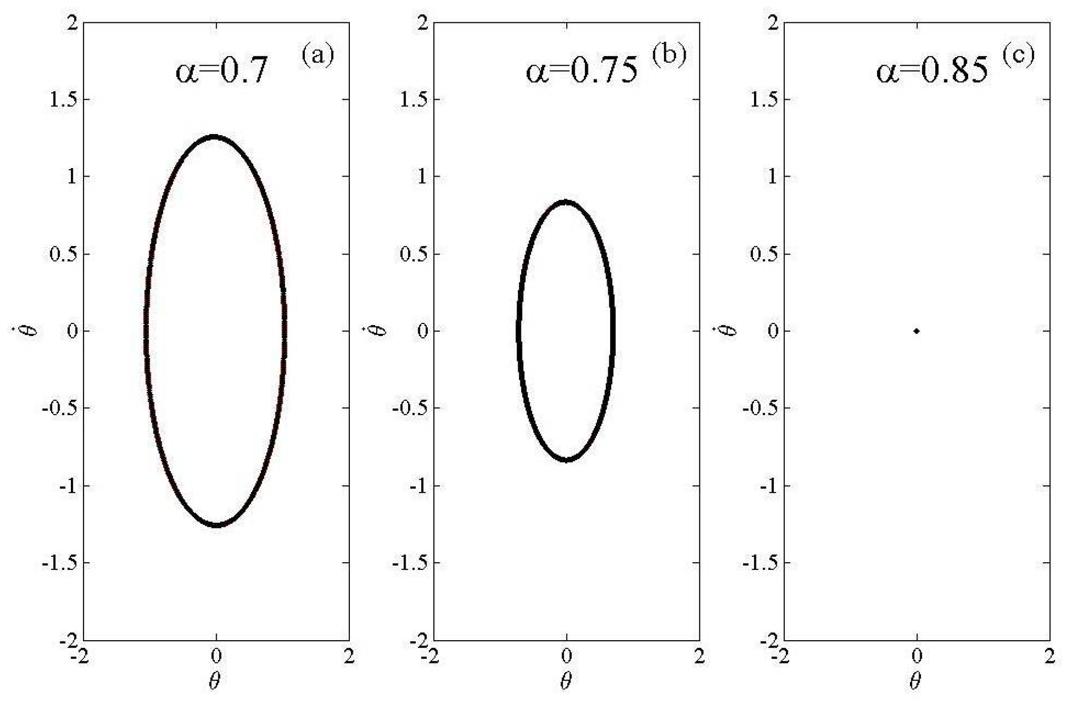
The phase diagrams with fractional order of 0.7, 0.75, 0.85 are depicted in
Figure 2. The time history diagram with fractional orders of 0.7, 0.75, 0.85 are depicted in
Figure 3. In
Figure 2 and
Figure 3, the same representative initial condition
are selected. A scrutiny of
Figure 2 and
Figure 3 indicates that the phase diagram the rolling mill’s main drive system changes from a limit cycle to a stable steady state along with the increase in the fractional order. This confirms the validity of our research results.
5. Stochastic Case
As is well known, noise is omnipresent in many dynamics systems. Therefore, it is important to study the response of the the rolling mill’s main drive system in the presence of noise. Subsequently, the effect of noise intensity and fractional order will be investigated in the rolling mill’s main drive system. The parameters are fixed.
5.1. Effect of Noise Intensity
The effects of noise intensity
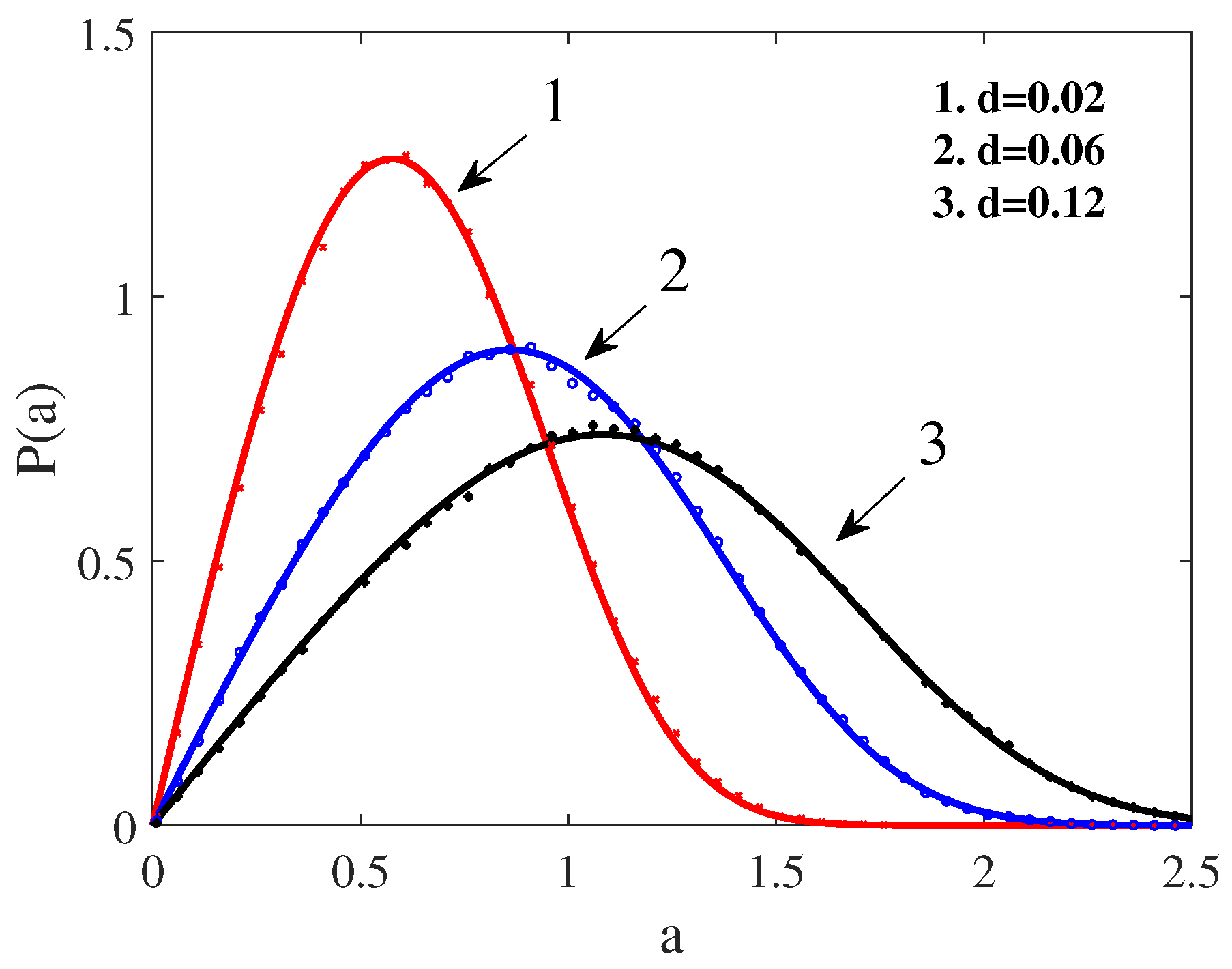
d on the rolling mill’s main drive system will be studied in this part. The theoretical results and numerical results of the stationary probability density function (PDF)
and joint stationary probability density function
are obtained and shown in
Figure 4 and
Figure 5.
As can be seen from
Figure 4, the stationary PDF
for different noise intensity showed a unimodal shape. Firstly, for noise intensity
, the peak of the stationary PDF
corresponds to a smaller amplitude (see curve 1). For noise intensity
, the amplitude corresponding to the peak of the stationary PDF becomes larger(see curve 2). With the noise intensity further increase (
), the amplitude corresponding to the peak of the PDF still increases further (see curve 3). This implies that the system response is concentrated near a certain amplitude in the presence of noise and increases gradually with the monotonically increasing of noise intensity.
5.2. Effect of Fractional Order
The effects of fractional order on the rolling mill’s main drive system have been studied in this subsection. The theoretical results and numerical results of the stationary PDF
and joint stationary PDF
are obtained and shown
Figure 6 and
Figure 7.
It reflects that both the stationary PDF
for different noise intensities showed a unimodal shape in
Figure 6. Firstly, for fractional order
, the peak of the stationary PDF
corresponds to a larger amplitude (see curve 1). For fractional order
, the amplitude corresponding to the peak of the stationary PDF
becomes smaller (see curve 2). With the fractional order further increasing (
, see curve 3), the amplitude corresponding to the peak of the stationary PDF
still decreases further. This implies that the system response is concentrated near a certain amplitude in the presence of noise and decreases gradually with the monotonically increasing of fractional order.
To conclude, all of the above results mirror that noise intensity and fractional order can modulate the amplitude corresponding to the peak of the stationary PDF’s left shift or right shift. The evolution of the response with the monotonic increasing of noise intensity and fractional order indicate that the noise intensity is conducive to modulate a larger amplitude. In contrast, the fractional order is conducive to induce a small amplitude.
It is worth pointing out that the response of the rolling mill’s main drive system for different fractional orders yields a limit cycle or a stable fixed point in the absence of noise. Nevertheless, both the stationary probability density functions for different system parameters (noise intensity and fractional order) showed a unimodal shape in the presence of noise. The theoretical and numerical results of the stationary probability density function and joint stationary probability density function verify the validity of the conclusion.
6. Conclusions and Discussion
In a summary, the rolling mill’s main drive system with a fractional order derivative and stochastic disturbance was considered. The dynamics of the rolling mill’s main drive system was investigated both in the absence and in the presence of stochastic disturbance.
For the absence of stochastic disturbance, the deterministic bifurcations induced by fractional order were explored based on the linearization method and a numerical simulation for the rolling mill’s main drive system. The results indicated that fractional order can change the system from a stable point to a limit cycle.
For the presence of stochastic disturbance, the response of the rolling mill’s main drive system was investigated with varying the fractional order and noise intensity. The evolution of the response with the monotonic increase in noise intensity and fractional order implied that the noise intensity was conducive to modulate a larger amplitude. In contrast, the fractional order was conducive to induce a small amplitude. Therefore, it provides an efficient strategy to control the system so that the amplitude of the vibration was small enough when the vibration occurs, which is going to be our later work.
In this paper, the rolling mill’s main drive system with fractional order and stochastic disturbance is considered and the dynamic response is investigated both in the absence and presence of stochastic disturbance. We mainly focused on the impact of Gaussian white noise and fractional order on the dynamic behavior of the system. The impact of other types of noise and time delays on the dynamic behavior of the system is also a problem that needs further research.
Author Contributions
Formal analysis, G.W.; methodology, G.W.; writing—original draft preparation, G.W.; writing—review and editing, G.W. and L.M.; supervision, L.M. All authors have read and agreed to the published version of the manuscript.
Funding
This work is supported by the National Natural Science Foundation of China (Grant No. U1910213).
Institutional Review Board Statement
Not applicable.
Informed Consent Statement
Not applicable.
Data Availability Statement
Not applicable.
Conflicts of Interest
The authors declare no conflict of interest.
References
- Mao, D.H.; Zhang, Y.F.; Nie, Z.H.; Liu, Q.H.; Zhong, J. Effects of ultrasonic treatment on structure of roll casting aluminum strip. J. Cent. South Univ. Technol. 2007, 14, 363–369. [Google Scholar] [CrossRef]
- He, J.; Yu, S.; Zhong, J. Modeling for driving systems of four-high rolling mill. Trans. Nonferrous Met. Soc. China 2002, 12, 88–92. [Google Scholar]
- Yarita, K.; Furukawa, K.; Seino, Y.; Takimoto, T.; Nakazato, Y.; Nakagawa, K. An analysis of chattering in cold rolling for ultrathin gauge steel strip. Trans. Iron Steel Inst. Jpn. 1978, 18, 1–10. [Google Scholar] [CrossRef]
- Tlusty, J.; Chandra, G.; Critchley, S.; Paton, D. Chatter in cold rolling. Cirp Ann. 1982, 31, 195–199. [Google Scholar] [CrossRef]
- Chefneux, L.; Fischbach, J.P.; Gouzou, J. Study and industrial control of chatter in cold rolling. Iron Steel Eng. 1984, 61, 17–26. [Google Scholar]
- Dhaouadi, R.; Kubo, K.; Tobise, M. Two-degree-offreedom robust speed controller for high-performance rolling mill drives. IEEE Trans. Ind. Appl. 1993, 29, 919–926. [Google Scholar] [CrossRef]
- Wang, Z.; Wang, D. Dynamic characteristics of a rolling mill drive system with backlash in rolling slippage. J. Mater. Process. Technol. 2000, 97, 69–73. [Google Scholar] [CrossRef]
- Kashay, A.M. Torque Amplification and Vibration Investigation Project. Iron Steel Eng. 1973, 50, 55–70. [Google Scholar]
- Klamka, J. Torque amplification and torsional vibration in large reversing mill drive. Iron Steel Eng. 1969, 5, 54–66. [Google Scholar]
- Ding, Q.; Cooper, J.E.; Leung, A.Y.T. Hopf bifurcation analysis of a rotor/seal system. J. Sound Vib. 2002, 252, 817–833. [Google Scholar] [CrossRef]
- Zhang, R.; Yang, P.; Cui, C. Hopf bifurcation for nonlinear delay system of rolling mill main drive. J. Vib. Meas. Diagn. 2014, 234, 909–914. [Google Scholar]
- Mainardi, F. Fractional Calculus and Waves in Linear Viscoelasticity: An Introduction to Mathematical Models; World Scientific: Singapore, 2010. [Google Scholar]
- Caponetto, R. Fractional Order Systems: Modeling and Control Applications; World Scientific: Singapore, 2010. [Google Scholar]
- Monje, C.A.; Chen, Y.; Vinagre, B.M.; Xue, D.; Feliu-Batlle, V. Fractional-Order Systems and Controls: Fundamentals and Applications; Springer Science & Business Media: Berlin/Heidelberg, Germany, 2010. [Google Scholar]
- Carpinteri, A.; Mainardi, F. Fractals and Fractional Calculus in Continuum Mechanics; Springer: Berlin/Heidelberg, Germany, 2014; p. 378. [Google Scholar]
- Rossikhin, Y.A.; Shitikova, M.V. Application of fractional calculus for dynamic problems of solid mechanics: Novel trends and recent results. Appl. Mech. Rev. 2010, 63, 010801. [Google Scholar] [CrossRef]
- Agrawal, O.P. A general formulation and solution scheme for fractional optimal control problems. Nonl. Dyn. 2004, 38, 323–337. [Google Scholar] [CrossRef]
- Ozaktas, H.M.; Kutay, M.A. 2001 European Control Conference (ECC); IEEE: Piscataway, NJ, USA, 2001; pp. 1477–1483. [Google Scholar]
- Das, S.; Pan, I. Fractional Order Signal Processing: Introductory Concepts and Applications; Springer Science & Business Media: Berlin/Heidelberg, Germany, 2011. [Google Scholar]
- Kusnezov, D.; Bulgac, A.; Do Dang, G. Quantum levy processes and fractional kinetics. Phys. Rev. Lett. 1999, 82, 1136. [Google Scholar] [CrossRef] [Green Version]
- Rossikhin, Y.A.; Shitikova, M.V. Analysis of damped vibrations of linear viscoelastic plates with damping modeled with fractional derivatives. Signal Process. 2006, 86, 2703–2711. [Google Scholar] [CrossRef]
- Xie, J.; Zheng, Y.; Ren, Z.; Wang, T.; Shen, G. Numerical vibration displacement solutions of fractional drawing self-excited vibration model based on fractional Legendre functions. Complexity 2019, 2019, 9234586. [Google Scholar] [CrossRef] [Green Version]
- Wang, J.; Ma, L.; Wang, Y. Hopf bifurcation control for the main drive delay system of rolling mill. Adv. Differ. Equ. 2020, 2020, 211. [Google Scholar] [CrossRef]
- Duan, J.Q. An Introduction to Stochastic Dynamics; Cambridge University Press: Cambridge, UK, 2015. [Google Scholar]
- Liu, J.K.; Xu, W. An averaging result for impulsive fractional neutral stochastic differential equations. Appl. Math. Lett. 2021, 114, 106892. [Google Scholar] [CrossRef]
- Liu, J.K.; Wei, W.; Xu, W. An averaging principle for stochastic fractional differential equations driven by fBm involving impulses. Fractal Fract. 2022, 6, 256. [Google Scholar] [CrossRef]
- Zakharova, A.; Vadivasova, T.; Anishchenko, V.; Koseska, A.; Kurths, J. Stochastic bifurcations and coherencelike resonance in a self-sustained bistable noisy oscillator. Phys. Rev. E 2010, 81, 011106. [Google Scholar] [CrossRef]
- Jin, C.; Sun, Z.K.; Xu, W. Stochastic bifurcations and its regulation in a Rijke tube model. Chaos Soliton Fract 2022, 154, 111650. [Google Scholar] [CrossRef]
- Liu, J.; Wei, W.; Wang, J.; Xu, W. Limit behavior of the solution of Caputo-Hadamard fractional stochastic differential equations. Appl. Math. Lett. 2023, 140, 108586. [Google Scholar] [CrossRef]
- Xu, B.Y.; Wang, X.D.; Liu, Y.L.; Feng, H.C. Strip Rolling Mill Random Vibration Analysis Based on Pseudo-Excitation Method. Appl. Mech. Mater. 2012, 143, 250–254. [Google Scholar]
- Xu, B.Y.; Liu, Y.L.; Wang, X.D.; Dong, F. Stochastic Excitation Model of Strip Rolling Mill. Appl. Mech. Mater. 2011, 216, 378–382. [Google Scholar]
- Shen, Y.J.; Wei, P.; Yang, S.P. Primary resonance of fractional-order van der Pol oscillator. Nonlinear Dyn. 2014, 77, 1629–1642. [Google Scholar] [CrossRef]
- Yang, Y.; Xu, W.; Gu, X.D. Stochastic response of a class of self-excited systems with Caputo-type fractional derivative driven by Gaussian white noise. Chaos Soliton Fract 2015, 77, 190–204. [Google Scholar] [CrossRef]
- Zhu, W.Q.; Lin, Y.K. Stochastic averaging of energy envelope. J. Eng. Mech. 1991, 117, 1890–1905. [Google Scholar] [CrossRef]
- Gu, X.; Zhu, W. A stochastic averaging method for analyzing vibro-impact systems under Gaussian white noise excitations. J. Sound. Vib. 2014, 333, 2632–2642. [Google Scholar] [CrossRef]
Figure 1.
Bifurcation diagram of the deterministic system for ; The red curve denotes the edge of the Hopf bifurcation.
Figure 1.
Bifurcation diagram of the deterministic system for ; The red curve denotes the edge of the Hopf bifurcation.
Figure 2.
Phase planes of the deterministic system for different fractional order: (a) , the system yields a large limit cycle; (b) , the system yields a small limit cycle; (c) , the system yields a stable steady state.
Figure 2.
Phase planes of the deterministic system for different fractional order: (a) , the system yields a large limit cycle; (b) , the system yields a small limit cycle; (c) , the system yields a stable steady state.
Figure 3.
The time history diagram of in the deterministic system: (a) ; (b) ; (c) .
Figure 3.
The time history diagram of in the deterministic system: (a) ; (b) ; (c) .
Figure 4.
The stationary probability density function of the amplitude for different noise intensity d with . The lines denote the analytical results, whereas dots represent the numerical results.
Figure 4.
The stationary probability density function of the amplitude for different noise intensity d with . The lines denote the analytical results, whereas dots represent the numerical results.
Figure 5.
The joint stationary probability density function with different noise intensity d. The the left side of the figure represent the analytic results and the right side denotes the numerical results.
Figure 5.
The joint stationary probability density function with different noise intensity d. The the left side of the figure represent the analytic results and the right side denotes the numerical results.
Figure 6.
The stationary probability density function of the amplitude for different fractional order with . The lines denote the analytical results, whereas dots represent the numerical results.
Figure 6.
The stationary probability density function of the amplitude for different fractional order with . The lines denote the analytical results, whereas dots represent the numerical results.
Figure 7.
The joint stationary probability density function with distinct values of . The left side of the figure represent the analytic results and the right side denotes the numerical results.
Figure 7.
The joint stationary probability density function with distinct values of . The left side of the figure represent the analytic results and the right side denotes the numerical results.
| Disclaimer/Publisher’s Note: The statements, opinions and data contained in all publications are solely those of the individual author(s) and contributor(s) and not of MDPI and/or the editor(s). MDPI and/or the editor(s) disclaim responsibility for any injury to people or property resulting from any ideas, methods, instructions or products referred to in the content. |
© 2023 by the authors. Licensee MDPI, Basel, Switzerland. This article is an open access article distributed under the terms and conditions of the Creative Commons Attribution (CC BY) license (https://creativecommons.org/licenses/by/4.0/).


