A Novel Fractional-Order Memristive Chaotic Circuit with Coexisting Double-Layout Four-Scroll Attractors and Its Application in Visually Meaningful Image Encryption

Abstract

This paper proposes a fractional-order chaotic system using a tri-stable locally active memristor. The characteristics of the memristor, dynamic mechanism of oscillation, and behaviors of the proposed system were analyzed, and then a visually meaningful image encryption scheme was designed based on the chaotic system, DNA encoding, and integer wavelet transform (IWT). Firstly, the mathematical model of the memristor was designed, which was nonvolatile, locally active, and tri-stable. Secondly, the stability, dynamic mechanism of oscillation, bifurcation behaviors, and complexity of the fractional-order memristive chaotic system were investigated and the conditions of stability were obtained. Thirdly, the largest Lyapunov exponent, bifurcation diagram, and complexity of the novel system were calculated and the coexisting bifurcation, coexisting attractors, spectral entropy, and so on are shown. Finally, a visually meaningful image encryption scheme based on the proposed system was designed, and its security was assessed by statistical analysis and different attacks. Numerical simulation demonstrated the effectiveness of the theoretical analysis and high security of the proposed image encryption scheme.

1. Introduction

Prof. Chua predicted that there should be four fundamental elements of the theory of completeness in nature, namely resistance, capacitance, inductance, and memristance [1]. As a possible component, initial research on memristors was slow and very few researchers were interested because there was no physical device to support memristance. With the development of technology, HP Labs first reported a physical device of a nano-size memristor in 2008, which was of groundbreaking significance [2]. From then on, research on memristors has attracted a huge amount of attention in industry and academia. Their natural nonlinear and non-volatile characteristics give memristors great potential for data storage and computation [3,4], artificial neural networks [5,6,7], nonlinear circuits [8,9,10], secure communication [11], image encryption [12,13,14], and other fields.

Chua proposed that local activity is the origin of complexity in 2005 [15]. The first locally active memristor was designed and called the Chua corsage memristor [16]. In order to analyze the characteristics of the memristor, some new methods such as DC V-I Plot, Power-Off Plot (POP), and Dynamic Route Map (DRM) were proposed. These methods can analyze the locally active and non-volatile characteristics of the memristor. Research showed that the memristor has negative differential memristance or memductance in some regions, called locally active memristors [17]. According to the conservation of energy, a memristive system can produce and maintain continuous self-excited oscillation in the locally active regions of the memristor, resulting in rich dynamic behaviors.

Recently, research on locally active memristors and their applications are going through a blowout period. In 2013, a NbO₂ Mott locally active memristor was first realized by Williams et al. [18]. Later, in 2021, the Williams team used a resistor, capacitor, and NbO₂ Mott locally active memristor to build a neuron chaotic system and analyzed the dynamic behaviors of the neuron system. Their research indicated that the physical locally active memristor could greatly improve the efficiency and accuracy of the computation when it was applied in a Hopfield neural network [19]. In 2016, Mannan et al. demonstrated a nonautonomous system based on the Chua corsage memristor and analyzed the edge of chaos and the Hopf bifurcation of the system. The results showed that the system would oscillate near locally active operating points located on the memristor’s DC V-I curve [16]. In 2017, Mannan et al. further studied the Chua corsage memristor and found that the memristor has two asymptotically stable equilibrium points and two distinct coexisting pinched hysteresis loops [20]. In 2018, Mannan et al. designed 4-lobe Chua corsage memristor and a 6-lobe Chua corsage memristor and analyzed their characteristics [21,22]. In 2020, Mannan et al. reviewed the nonlinear dynamic attributes, switching kinetics, bifurcation analysis, and physical realization of a family of Chua corsage memristors and analyzed the nonautonomous system based on the Chua corsage memristors, finding unique stable limit cycles from a supercritical Hopf bifurcation along with static attractors [23]. We find that all systems based on locally active memristors only produce periodic oscillations and no chaotic oscillations. In 2020, Dong et al. designed a bistable nonvolatile locally active memristor and added an inductor to the periodic oscillating circuit of the memristor. The coexisting chaotic attractors and various complex dynamic phenomena were reported in [24]. Tan et al. designed a simple locally active memristor and established HR neurons on the memristor. Complicated firing behaviors and coexisting position symmetry for different attractors were found in [25]. All of these studies showed that the locally active memristor has extensive application prospects and potential in chaotic oscillations.

As we all know, almost all systems are fractional-order systems in nature, and the integer-order system is a special case of fractional-order systems. Fractional calculus has the same historical memory function as a memristor; therefore, all memristive systems can be extended to fractional order. However, research on fractional-order chaotic systems based on locally active memristors is still in its infancy. Xie et al. proposed a fractional-order chaotic system based on a designed locally active memristor model, and dynamics analysis indicated that the system not only had diverse nonlinear dynamics, such as infinitely many discrete equilibrium points, multistability, and anti-monotonicity, but it also produced two new phenomena [26]. Ding et al. designed a fractional-order Hopfield neural network system based on a coupled locally active memristor, and the simulation results displayed that the fractional-order system not only had rich dynamic phenomena but also had some special transient transition process [27]. Yang et al. devised a fractional-order simplest chaotic system based on a bi-stable locally active memristor. Rich coexisting phenomena were found and some transient transition behaviors were analyzed [28]. It can be found that fractional-order systems based on locally-active memristors can generate richer dynamic behaviors and some new phenomena that have not been found in other chaotic systems.

Nowadays, digital images are ubiquitous, and yet the security of their transmission and storage causes anxiety. Research shows that there is higher security for image encryption in a chaotic system, which has better security than other methods because of the initial value sensitivity as well as the pseudo-random and aperiodic characteristics of chaotic systems. In recent years, many image encryption schemes based on chaotic systems have been proposed; however, these ciphertext images are noise-like or texture-like and easily distinguished from normal visually meaningful images. These visually meaningless noise-like images can only protect the security of image data but they fail to protect the security of image visual data. In pursuit of dual security of image data and visual data, the noise-like or texture-like ciphertext image should be converted into a visually meaningful image after the plain image is encrypted by existing encryption algorithms.

In order to achieve visual security, Bao et al. first proposed an image encryption scheme to encrypt plain images into visually meaningful ciphertext images [29]. This scheme added an embedding process on the basis of the existing image encryption algorithm. When the visually meaningful cipher image emerged in an insecure channel, it was difficult to catch the attention of attackers; therefore, the carrier image and the original image were more secure. Chai et al. proposed a novel visually secure image encryption scheme based on compressive sensing. Simulation results and performance analyses both demonstrated high sensitivity to the plain image and availability to known- and chosen-plaintext attacks [30]. Wang et al. proposed a visually meaningful scheme by employing the parallel compressive sensing method and embedding technique. Simulation analysis demonstrated that the cipher image exhibited excellent security and the reconstructed image had higher quality [31]. Ping et al. designed a visually meaningful image encryption scheme using the compressive sensing and partial block pairing substitution technique. Experimental results demonstrated that the scheme had higher quality and higher security [32]. It can be observed that the style of image decomposition is discrete wavelet transform (DWT); however, the DWT is irreversible, and the quality of the final reconstructed image will be poor during decryption. To solve this problem, the integer wavelet transform (IWT) is used to decompose and reconstruct the carrier image, which is fully reversible. Owing to the fact that IWT and inverse IWT are completely reversible, the obtained image is exactly the same as the original carrier image after the carrier image undergoes IWT and inverse IWT transformation. Based on this, we used this method to complete the embedding and extracting processes of the secret image.

Based on the above discussions, this study proposed a new continuous nonlinear tri-bistable locally active memristor model, and we studied its nonlinear characteristics. Then, we analyzed the features of the locally active memristor, including time-domain waveforms, three coexisting pinched hysteresis loops, Power-Off Plot, and DC V-I Curve. Next, we designed a fractional-order simple circuit system using our memristor, a linear passive inductor, and a linear passive capacitor in series. We observed that the system could produce oscillation under some conditions and had abundant dynamic behaviors. Finally, we used the fractional-order memristive chaotic system to design an image encryption scheme and analyzed its security. The contributions of this paper are listed as follows: (1) A tri-stable locally active memristor was designed and analyzed. (2) A fractional-order chaotic system was built based on the proposed memristor, and we discovered its rich coexisting dynamic behaviors. In order to apply the chaotic system, we analyzed the complexity when some parameters were changed. (3) A visually secure image encryption scheme was proposed based on the fractional-order memristive chaotic system and integer wavelet transform (IWT) embedding. The analysis results pointed out that our algorithm not had only higher security, but it also enabled dual protection of data security and visual security.

The remainder of this paper is organized as follows. The tri-stable locally-active memristor model is built in Section 2. Section 3 shows the dynamic characteristics of the designed memristor. The new fractional-order chaotic system based on the tri-stable locally-active memristor is presented, and the dynamic behavior of the chaotic system is analyzed in Section 4. Section 5 designs a visually meaningful image encryption scheme to use the chaotic system. Finally, Section 6 is the conclusion.

2. New Locally Active Memristor

Based on Chua’s definition and classification of memristors, this paper designed a new tri-stable locally-active memristor model, which can be described by the voltage–current relationship and the state equation as follows:

$$\frac{\mathrm{dx}}{\mathrm{dt}}={\mathrm{k}}_1\left(\mathrm{ax}+\mathrm{bx}\left|\mathrm{x}\right|+\mathrm{c}{\mathrm{x}}^3+\mathrm{dx}{\mathrm{v}}^2+\mathrm{ev}\right)$$

(1)

$$\mathrm{i}={\mathrm{k}}_2\left({\mathrm{x}}^2-\mathrm{m}\right)\mathrm{v}$$

(2)

where v and i are the input and output of the memristor, respectively. x is the state variable of the memristor. ${\mathrm{k}}_1$, ${\mathrm{k}}_2$, e, and m are parameters.

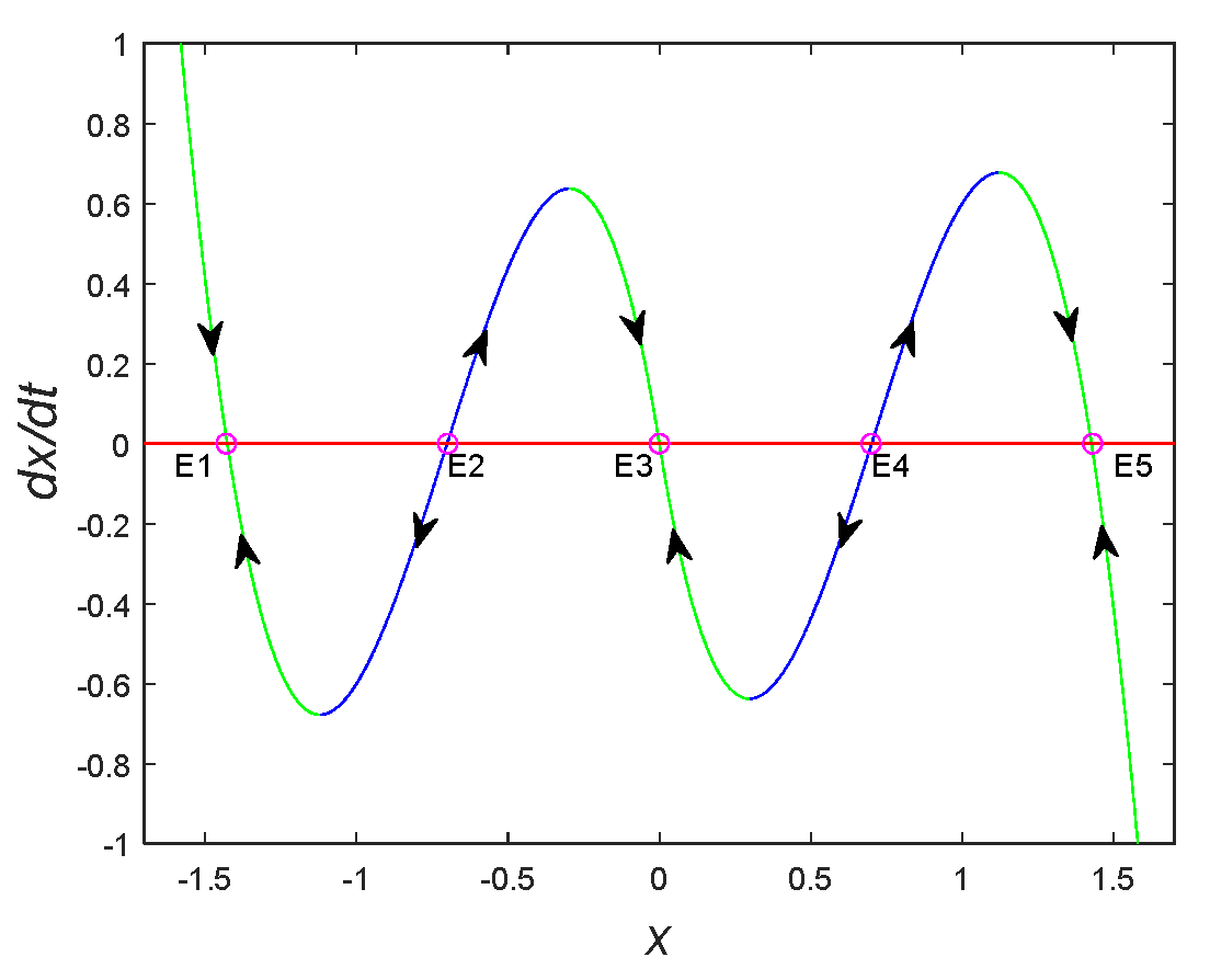
According to Equations (1) and (2), when the parameters are set as ${\mathrm{k}}_1=1,{\mathrm{k}}_2=1,\mathrm{a}=-4.7,\mathrm{b}=10,\mathrm{c}=-4.7,\mathrm{d}=0.1,\mathrm{m}=10,\mathrm{a}\mathrm{n}\mathrm{d}\mathrm{e}=10$, the color POP of Equation (1) with arrow heads is shown in Figure 1. It can be observed that there are five intersections with $\mathrm{d}\mathrm{x}/\mathrm{d}\mathrm{t}=0$, namely E₁, E₂, E₃, E₄, and E₅. By adjusting the dynamic route of the five points, we can judge that the equilibrium points E₁, E₃, and E₅ are asymptotically stable, whereas the equilibrium points E₂ and E₄ are unstable. The green lines represent the negative slope ranges, while the blue lines represent the positive slope ranges. The arrow above the x = 0 axis faces right, and the curve arrow below the x = 0 axis faces left.

2.1. Pinched Hysteresis Loops

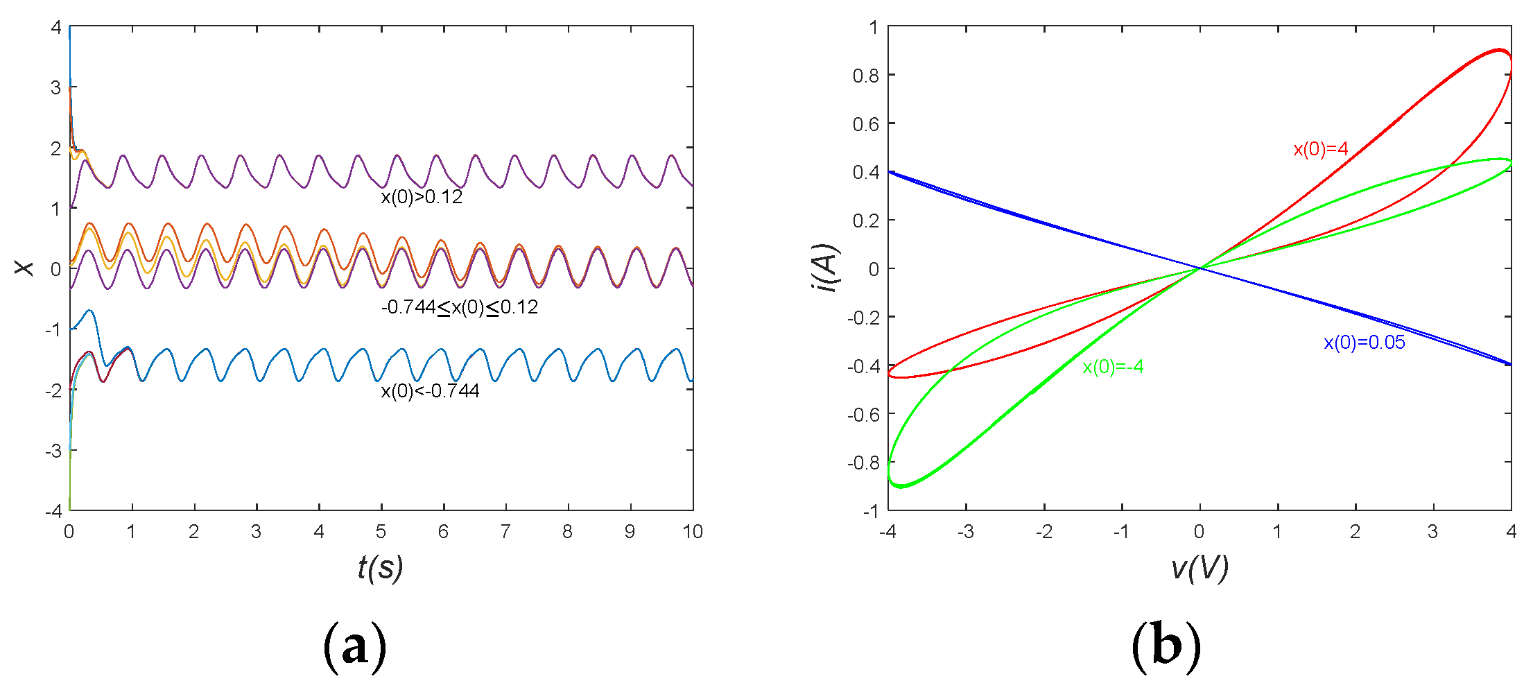
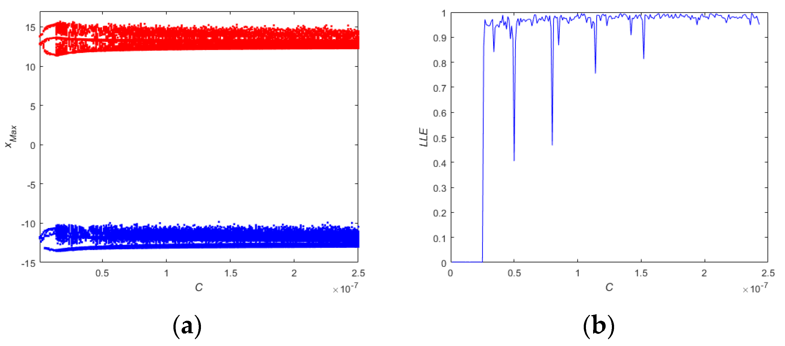
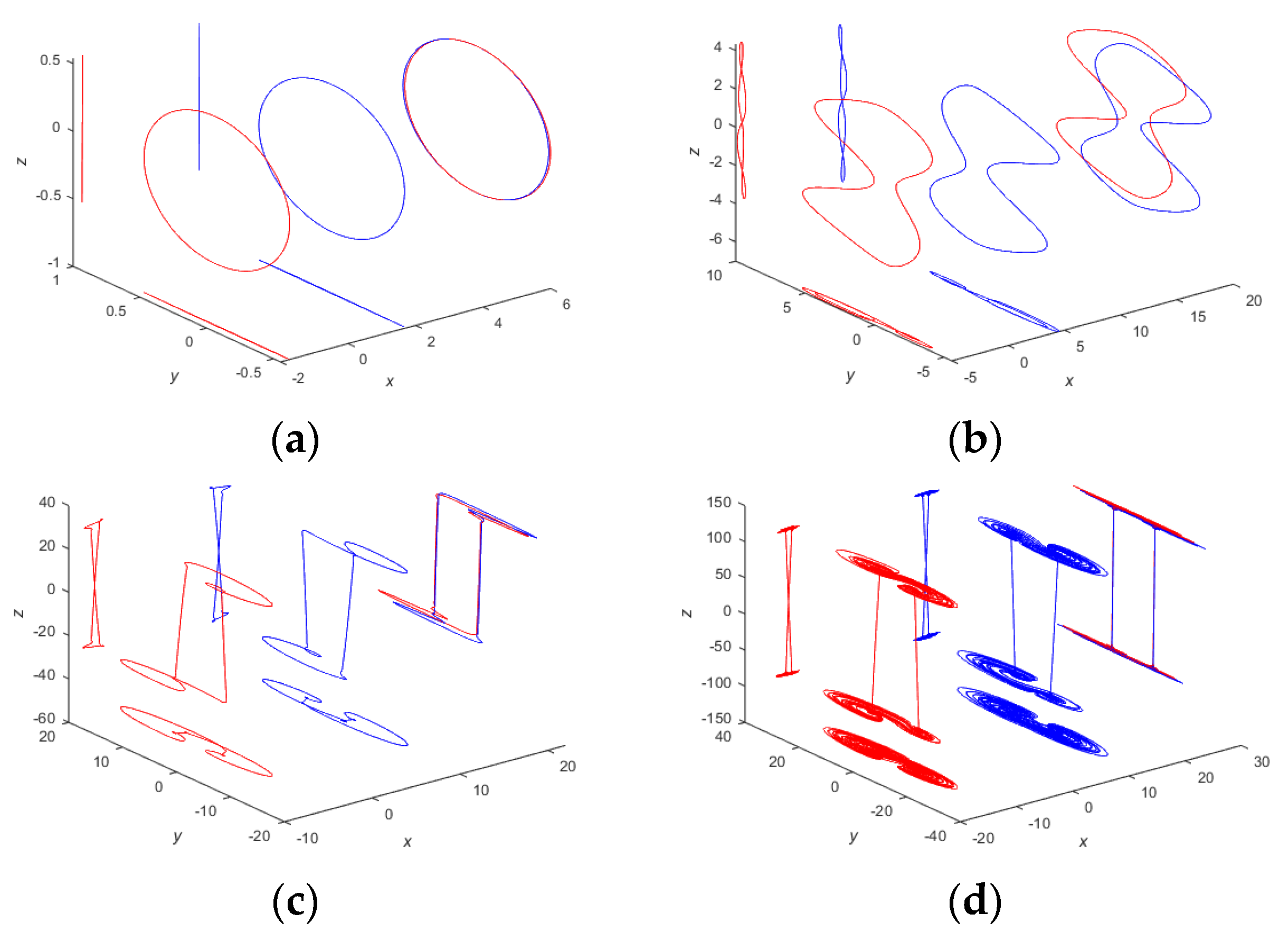
When the memristor is driven by a periodic signal source with amplitude A and frequency $\mathsf{\omega }$, the $\mathrm{v}-\mathrm{i}$ curves of the memristor are pinched hysteresis loops passing through the origin. While the parameters of the memristor and the periodic signal source take different values, and the initial values of Equation (1) also take different values, the memristor will exhibit a variety of characteristics. The parameters of Equations (1) and (2) are set as ${\mathrm{k}}_1=1,{\mathrm{k}}_2=1,\mathrm{a}=-4.7,\mathrm{b}=10,\mathrm{c}=-4.7,\mathrm{d}=0.1,\mathrm{m}=10,\mathrm{a}\mathrm{n}\mathrm{d}\mathrm{e}=10$.

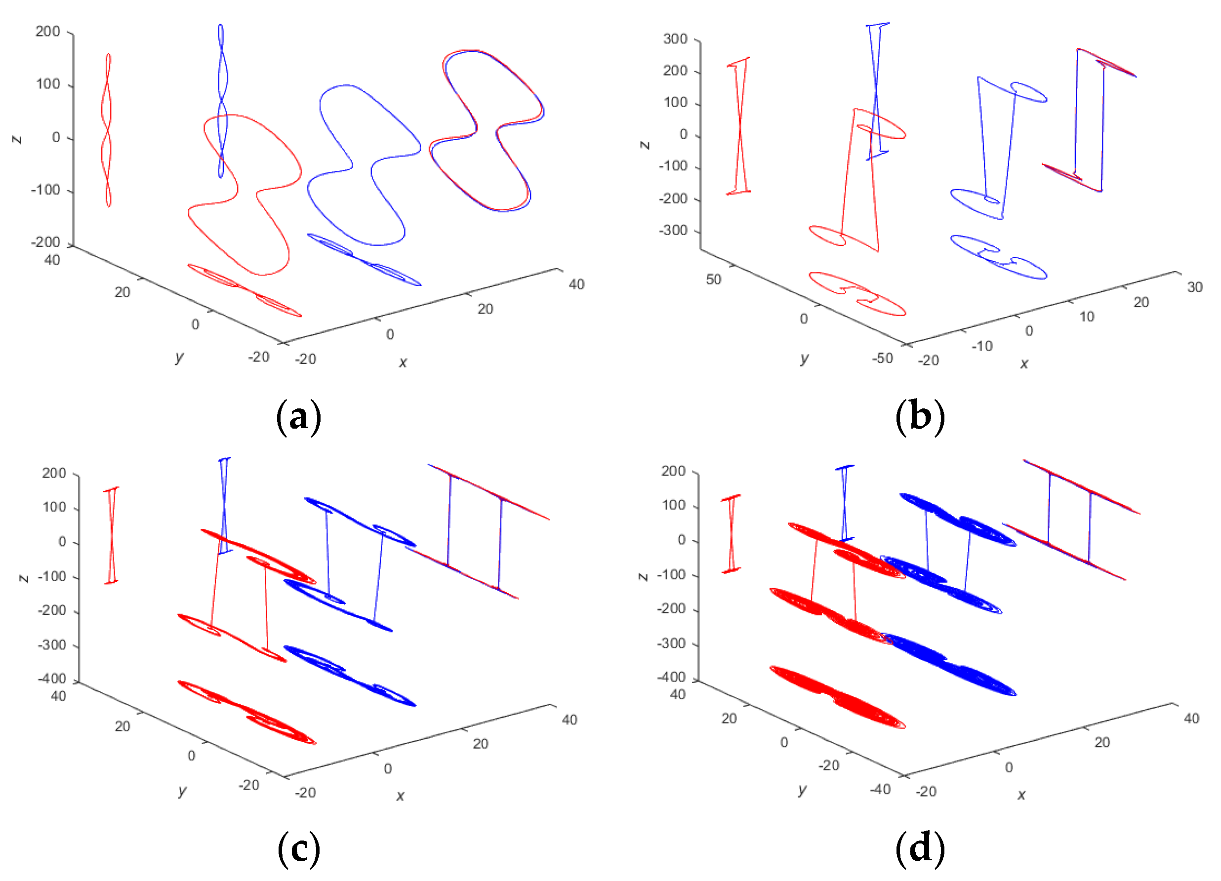
Let $\mathrm{A}=4,\mathsf{\omega }=10\mathrm{r}\mathrm{a}\mathrm{d}/\mathrm{s}$, and the parameter $\mathrm{d}$ is changed. When $d\in [-0.048,0.17]$, the dynamic trajectory displays three coexisting pinched hysteresis loops, as shown in Figure 2b, and the corresponding time-domain waveforms are shown in Figure 2a.

It can be observed from Figure 2 that if the initial value $\mathrm{x}\left(0\right)>0.12$, the pinched hysteresis loop is the red curve of Figure 2b; if the initial value $-0.744\le \mathrm{x}\left(0\right)\le 0.12$, the pinched hysteresis loop is the blue curve of Figure 2b; if the initial value $\mathrm{x}\left(0\right)<-0.744$, the pinched hysteresis loop is the green curve of Figure 2b. The red and green curves are symmetrical hysteresis loops about the origin. 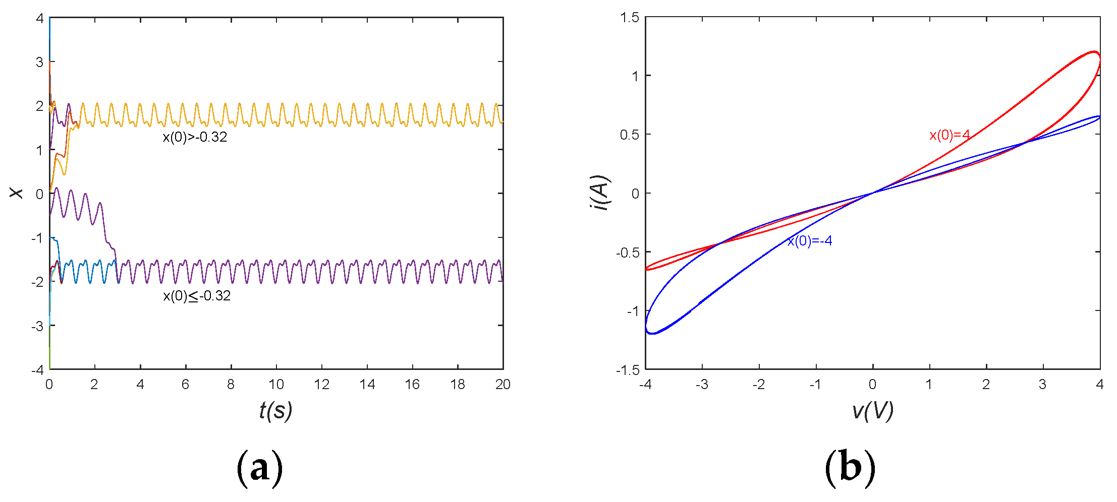When $\mathrm{d}>0.17$, the dynamic trajectories display double coexisting pinched hysteresis loops, as shown in Figure 3b, and the corresponding time-domain waveforms are shown in Figure 3a. It can be observed from Figure 3 that if the initial value $\mathrm{x}\left(0\right)>-0.32$, the pinched hysteresis loop is the red curve of Figure 3b; if the initial value $\mathrm{x}\left(0\right)<-0.32$, the pinched hysteresis loop is the green curve of Figure 3b. The red and blue curves are symmetrical hysteresis loops about the origin, and they have two pinched points. 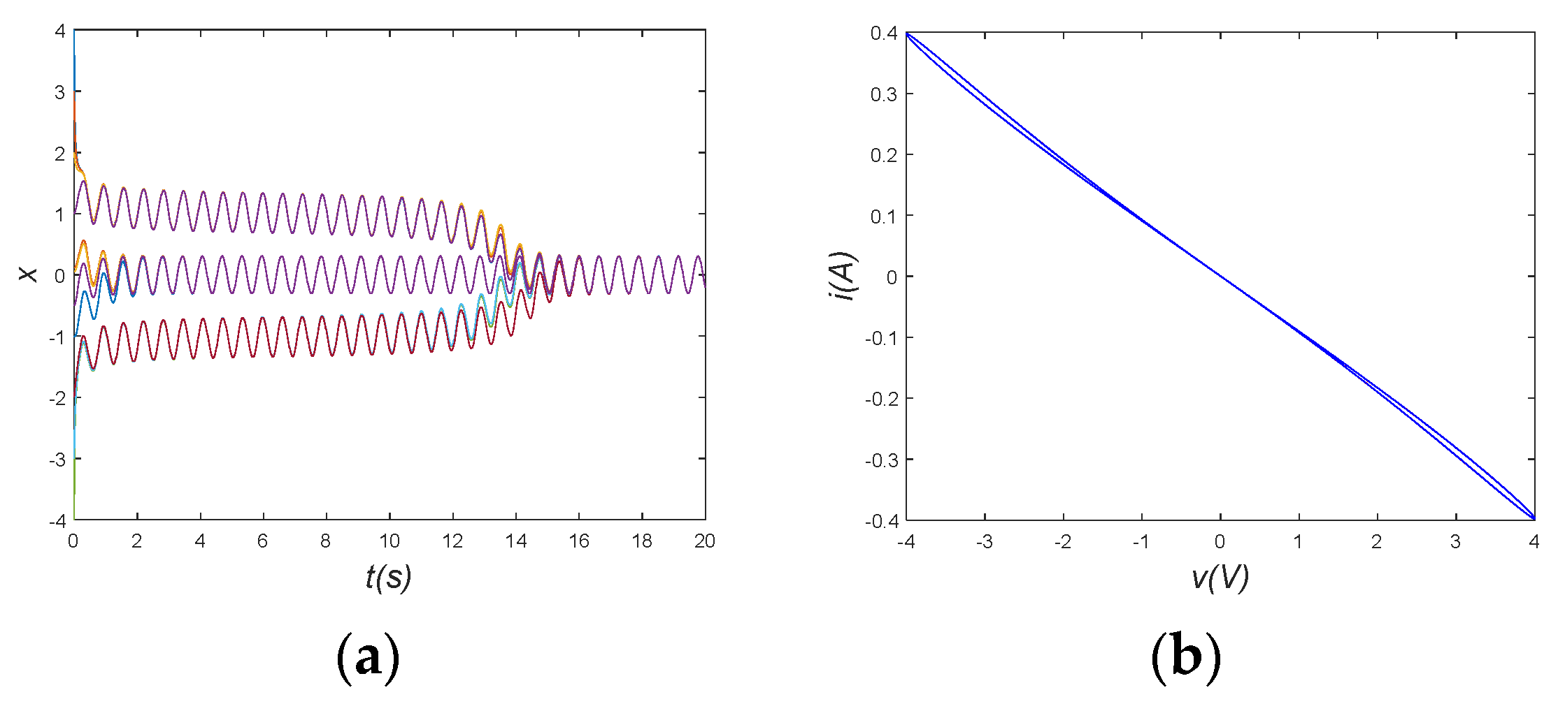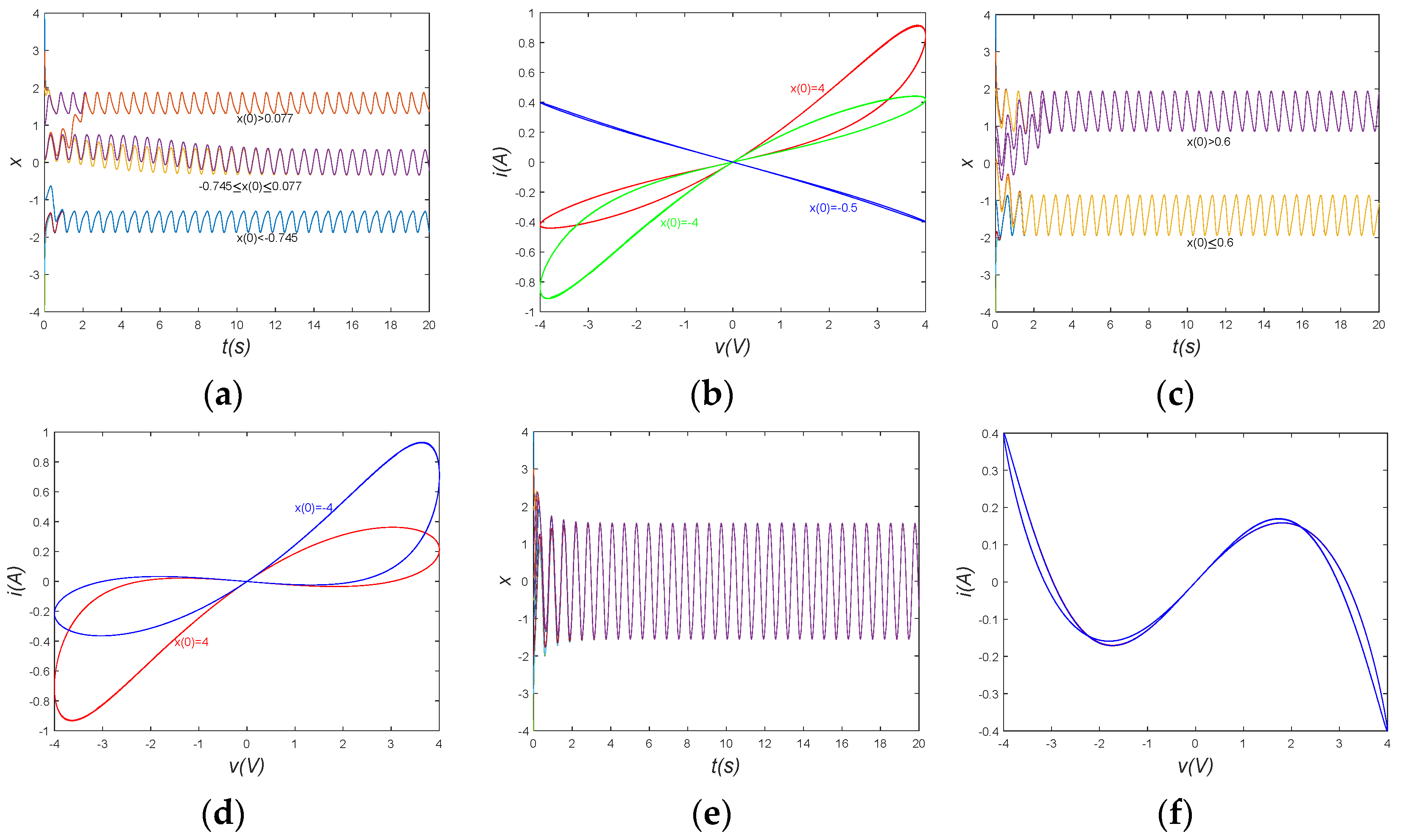When $\mathrm{d}<-0.048$, the dynamic trajectory displays only one pinched hysteresis loop, as shown in Figure 4b, and the corresponding time-domain waveforms are shown in Figure 4a. It can be observed that the dynamic trajectories have three stable states at the beginning, and as time goes on, the final curves are independent of the initial values and eventually converge to the same curve.

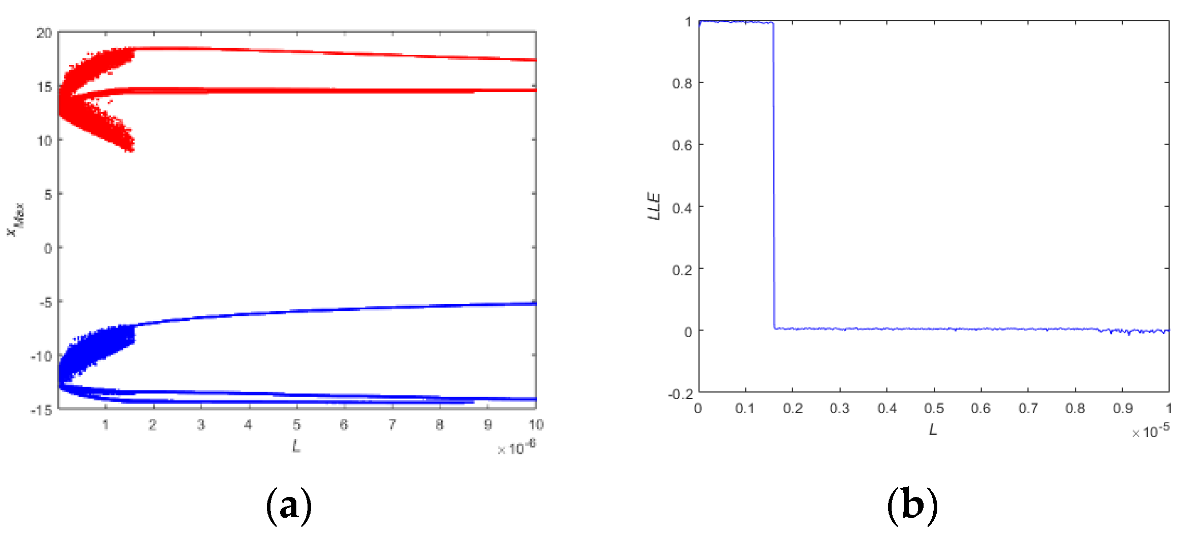
Let the amplitude $\mathrm{A}=4\mathrm{V},\mathsf{\omega }=10\mathrm{rad}/\mathrm{s}$, and the parameter $e$ is changed. When $\mathrm{e}\in \left[-1,0.958\right]$, the dynamic trajectory displays three coexisting pinched hysteresis loops, as shown in Figure 5b, and the corresponding time-domain waveforms are shown in Figure 5a. It can be observed from Figure 5 that if the initial value $\mathrm{x}\left(0\right)>0.077$, the pinched hysteresis loop is the red curve of Figure 5b; if the initial value −$0.745\le \mathrm{x}\left(0\right)\le 0.077$, the pinched hysteresis loop is the blue curve of Figure 5b; if the initial value $\mathrm{x}\left(0\right)<-0.745$, the pinched hysteresis loop is the green curve of Figure 5b. The red and green curves are symmetrical hysteresis loops about the origin. When $\mathrm{e}>0.958$ and −$3.6\le \mathrm{e}<-1$, the dynamic trajectories display double coexisting pinched hysteresis loops, as shown in Figure 5d, and the corresponding time-domain waveforms are shown in Figure 5c. It can be observed that if the initial value $\mathrm{x}\left(0\right)>0.6$, the pinched hysteresis loop is the red curve of Figure 5b; if the initial value $\mathrm{x}\left(0\right)\le 0.6$, the pinched hysteresis loop is the green curve of Figure 5b. The red and blue curves are symmetrical hysteresis loops about the origin, and they have two pinched points. When $\mathrm{e}>-3.6$, the dynamic trajectory displays only one pinched hysteresis loop, as shown in Figure 5f, and the corresponding time-domain waveforms are shown in Figure 5e. It can be observed that the pinched hysteresis loop has three pinched points and is symmetric about the origin.

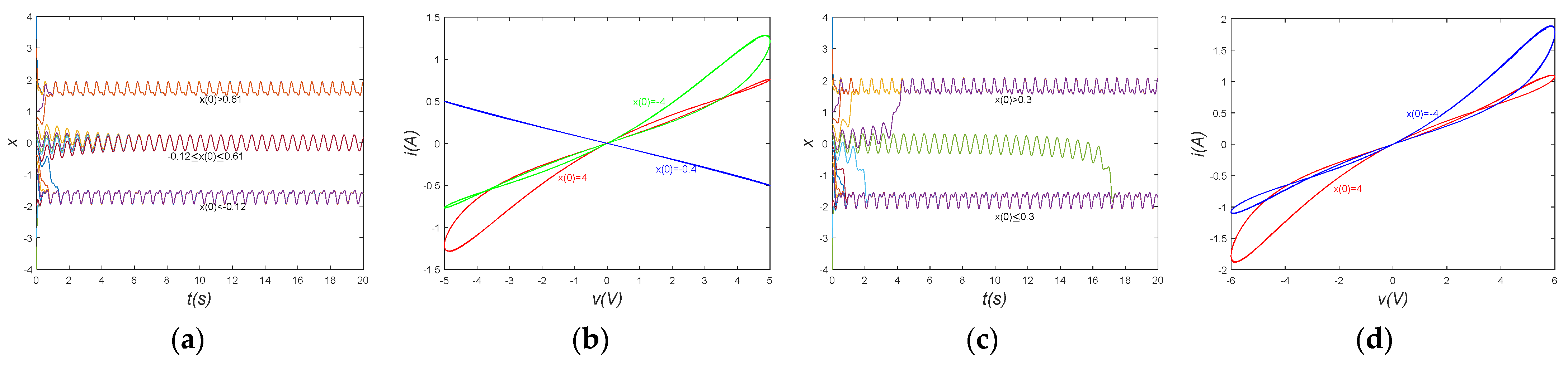
Let the amplitude $\mathrm{e}=0.5,\mathrm{d}=0.1,\mathsf{\omega }=10\mathrm{rad}/\mathrm{s}$, and the parameter $\mathrm{A}$ is changed. When $\mathrm{A}\le 5.7$, the dynamic trajectory displays three coexisting pinched hysteresis loops, as shown in Figure 6b, and the corresponding time-domain waveforms are shown in Figure 6a. It can be seen that if the initial value $\mathrm{x}\left(0\right)>0.61$, the pinched hysteresis loop is the red curve of Figure 6b; if the initial value −$0.12\le \mathrm{x}\left(0\right)\le 0.61$, the pinched hysteresis loop is the blue curve of Figure 6b; if the initial value $\mathrm{x}\left(0\right)<-0.12$, the pinched hysteresis loop is the green curve of Figure 6b. The red and green curves are symmetrical hysteresis loops about the origin. When $\mathrm{A}>5.7$, the dynamic trajectories display double coexisting pinched hysteresis loops, as shown in Figure 6d, and the corresponding time-domain waveforms are shown in Figure 6c. It can be observed that if the initial value $\mathrm{x}\left(0\right)>0.3$, the pinched hysteresis loop is the red curve of Figure 6d; if the initial value $\mathrm{x}\left(0\right)\le 0.3$, the pinched hysteresis loop is the green curve of Figure 6d. The red and blue curves are symmetrical hysteresis loops about the origin and they have two pinched points.

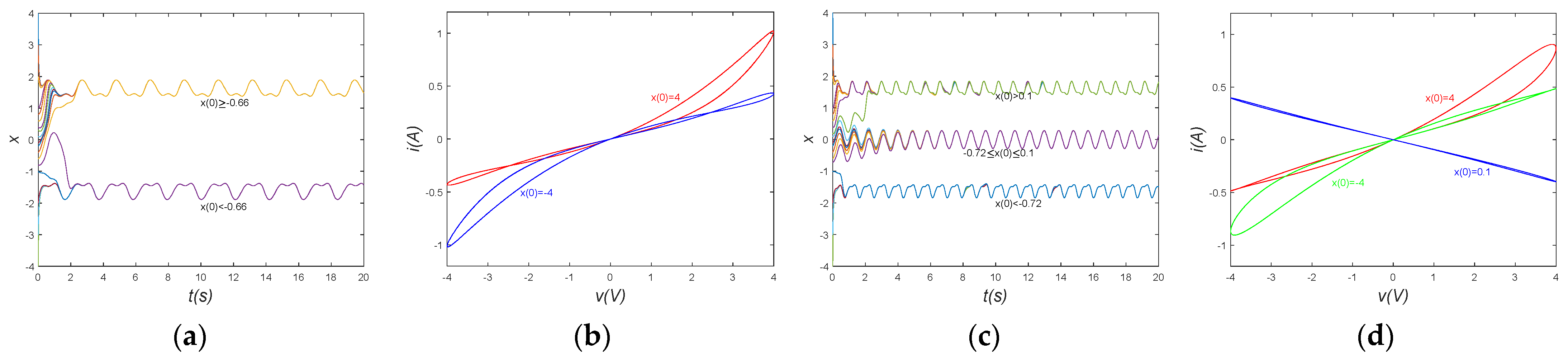
Let the amplitude $\mathrm{e}=0.5,\mathrm{d}=0.1,\mathrm{A}=4\mathrm{V}$, and the parameter $\mathsf{\omega }$ is changed. When $\mathsf{\omega }\le 5$, the dynamic trajectory displays double coexisting pinched hysteresis loops, as shown in Figure 7b, and the corresponding time-domain waveforms are shown in Figure 7a. It can be observed that if the initial value $\mathrm{x}\left(0\right)\ge -0.66$, the pinched hysteresis loop is the red curve of Figure 7b; if the initial value $\mathrm{x}\left(0\right)<-0.66$, the pinched hysteresis loop is the blue curve of Figure 7b. The red and green curves are symmetrical hysteresis loops about the origin. When $\mathsf{\omega }>5$, the dynamic trajectories display three coexisting pinched hysteresis loops, as shown in Figure 7d, and the corresponding time-domain waveforms are shown in Figure 7c. It can be observed that if the initial value $\mathrm{x}\left(0\right)>0.1$, the pinched hysteresis loop is the red curve of Figure 7d; if the initial value −$0.72\le \mathrm{x}\left(0\right)\le 0.1$, the pinched hysteresis loop is the blue curve of Figure 7d; if the initial value $\mathrm{x}\left(0\right)$ < $-0.72$, the pinched hysteresis loop is the green curve of Figure 7d. The red and blue curves are symmetrical hysteresis loops about the origin. It can be seen from the above analysis that the memristor presented different stable states with changes in parameters and input signals.

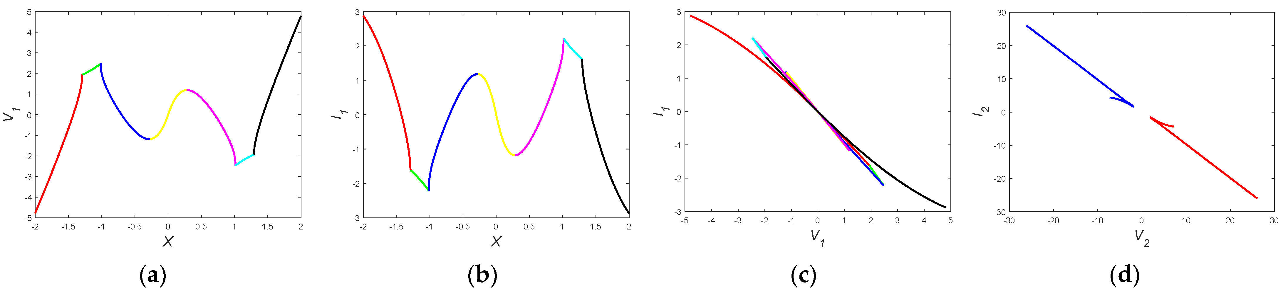
2.2. Local Activity

The DC V-I plot reflects Ohm’s law for the memristor, which describes the DC characteristics of the memristor and can analyze the intrinsic locally active features of the memristor. Let $\mathrm{x}=\mathrm{X},\mathrm{d}\mathrm{x}/\mathrm{d}\mathrm{t}{|}_{\mathrm{x}=\mathrm{X}}=0$ in Equation (1), we can obtain the relationship between voltage $V$ and state variable $X$:

$$\mathrm{aX}+\mathrm{bX}\left|\mathrm{X}\right|+\mathrm{c}{\mathrm{X}}^3+\mathrm{dX}{\mathrm{V}}^2+\mathrm{eV}=0$$

(3)

Then, setting $\mathrm{a}=-4.7,\mathrm{b}=10,\mathrm{c}=-4.7,\mathrm{d}=0.1,\mathrm{a}\mathrm{n}\mathrm{d}\mathrm{e}=0.5$. Based on Equation (3), we can obtain a function between the state variable $\mathrm{X}$ and the DC voltage $\mathrm{V}$:

$${\mathrm{V}}_1=\frac{-5+\sqrt{25+4\mathrm{X}\left(47\mathrm{X}-100\mathrm{X}\left|\mathrm{X}\right|+47{\mathrm{X}}^3\right)}}{2\mathrm{X}}$$

(4)

$${\mathrm{V}}_2=\frac{-5-\sqrt{25+4\mathrm{X}\left(47\mathrm{X}-100\mathrm{X}\left|\mathrm{X}\right|+47{\mathrm{X}}^3\right)}}{2\mathrm{X}}$$

(5)

Substituting Equations (4) and (5) into Equation (2), the DC current $\mathrm{I}$ can be calculated, respectively:

$${\mathrm{I}}_1=\left({\mathrm{X}}^2-\mathrm{m}\right){\mathrm{V}}_1$$

(6)

$${\mathrm{I}}_2=\left({\mathrm{X}}^2-\mathrm{m}\right){\mathrm{V}}_2$$

(7)

Let $\mathrm{m}=10$, based on Equations (4) and (6), when −$2<\mathrm{X}<2,$ we drew points $\left(\mathrm{X},{\mathrm{V}}_1\right),\left(\mathrm{X},{\mathrm{I}}_1\right),$ and $\left({\mathrm{V}}_1,{\mathrm{I}}_1\right)$ in the $\mathrm{X}-{\mathrm{V}}_1,\mathrm{X}-{\mathrm{I}}_1$ and ${\mathrm{V}}_1-{\mathrm{I}}_1$ planes, respectively, and obtained the DC ${\mathrm{V}}_1-{\mathrm{I}}_1$ plots shown in Figure 8a–c. Based on Equations (5) and (7), we drew points $\left({\mathrm{V}}_2,{\mathrm{I}}_2\right)$ in the ${\mathrm{V}}_2-{\mathrm{I}}_2$ plane and obtained the DC ${\mathrm{V}}_2-{\mathrm{I}}_2$ plot shown in Figure 8d in the same way. It was observed that the slopes of all of the curves had negative values; therefore, we determined that the memristor was a locally active memristor.

Comparison with the existing memristor model is shown in

Table 1. Comparison with the memristor model.

Memristor Models	Number of Parameters	Number of Equilibrium Points
Ref. [17]	1	3
Ref. [25]	1	3
Ref. [33]	2	infinite
Ref. [34]	1	5
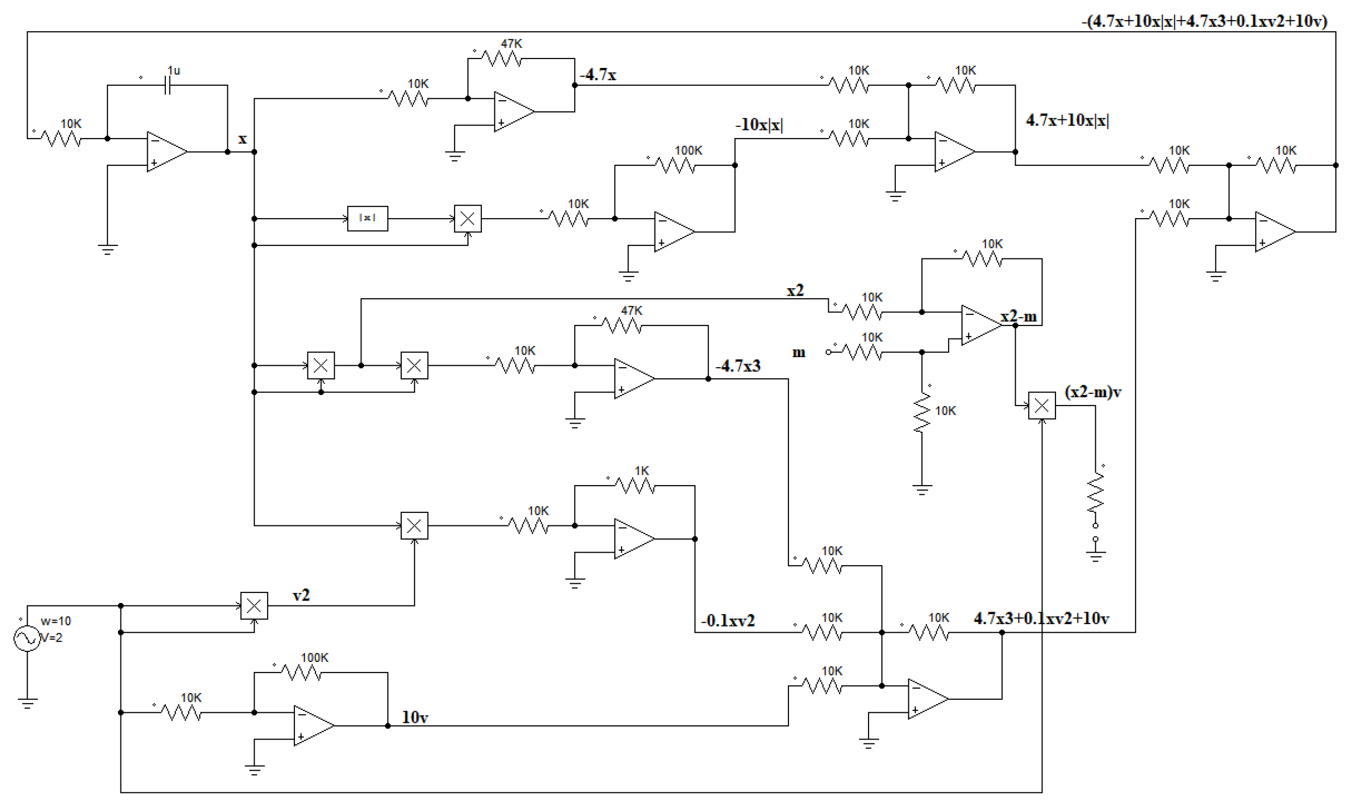
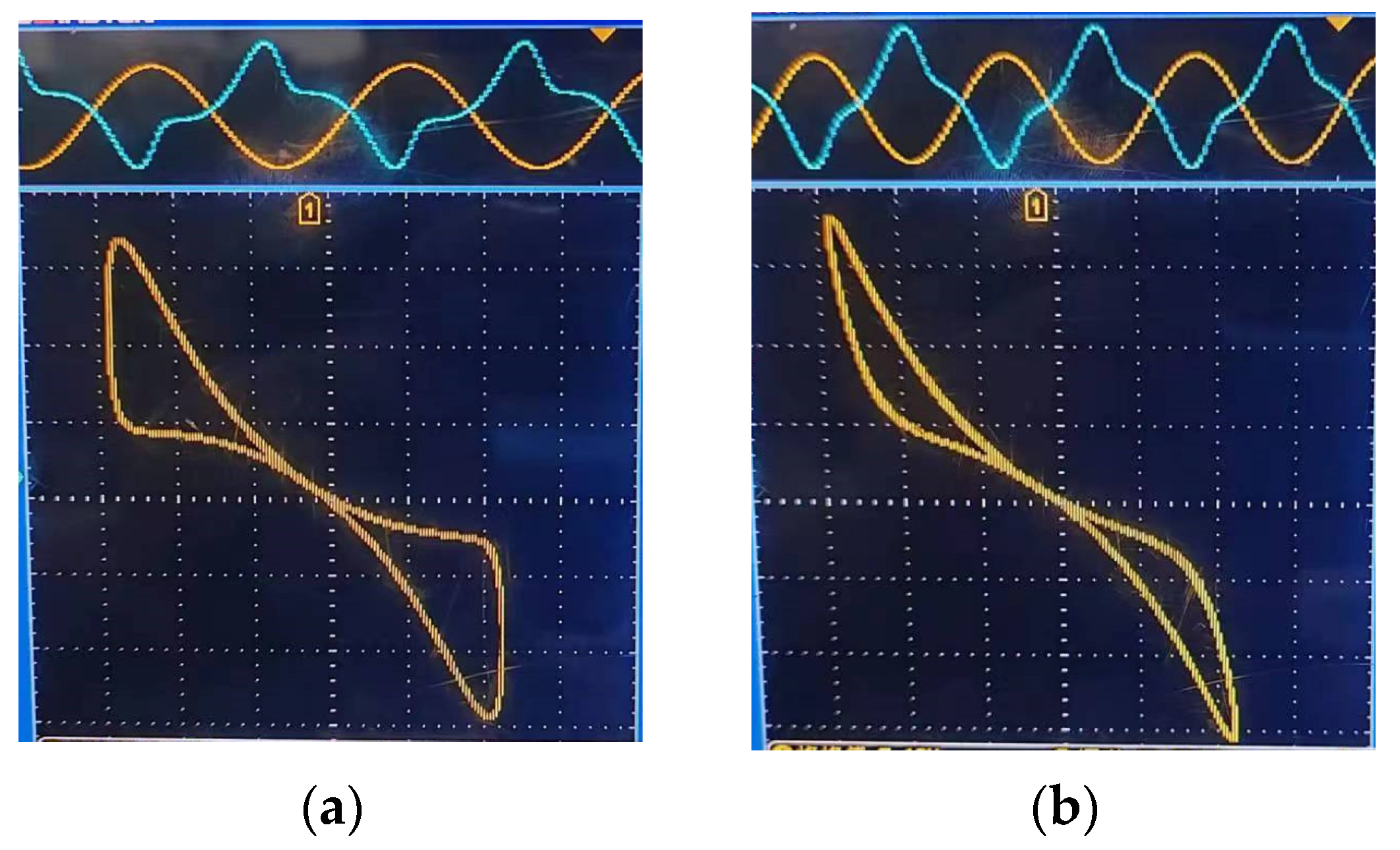
Ours	7	5

. It was found that the model proposed in this paper had more parameters and equilibrium points. In order to verify the correctness of the analysis, we designed a circuit on the proposed memristor, as shown in Figure 9. When we placed a sinusoidal excitation at both ends of the memristor, pinched hysteresis loops were observed, as shown in Figure 10. It could be concluded that the analysis was correct by comparison.

3. Fractional-Order Memristive Chaotic System

A fractional-order capacitor, fractional-order inductance, and our proposed fractional-order memristor were connected in series to construct a third-order fractional-order circuit, as shown in Figure 11. The new 3D fractional-order memristive system may generate chaotic oscillation because it contained a locally active memristor.

According to Kirchhoff’s laws, we could obtain the fractional-order differential equations as follows:

$$\left\{\begin{array}{l}\frac{{\mathrm{d}}^{\mathrm{q}}\mathrm{x}}{\mathrm{d}{\mathrm{t}}^{\mathrm{q}}}=\mathrm{k}\left(\mathrm{ax}+\mathrm{bx}\left|\mathrm{x}\right|+\mathrm{c}{\mathrm{x}}^3+\mathrm{ex}{\mathrm{y}}^2+\mathrm{fy}\right)\\ \frac{{\mathrm{d}}^{\mathrm{q}}\mathrm{y}}{\mathrm{d}{\mathrm{t}}^{\mathrm{q}}}=-\frac{\left({\mathrm{x}}^2-\mathrm{m}\right)\mathrm{y}+\mathrm{z}}{\mathrm{L}}\\ \frac{{\mathrm{d}}^{\mathrm{q}}\mathrm{z}}{\mathrm{d}{\mathrm{t}}^{\mathrm{q}}}=\frac{\mathrm{y}}{\mathrm{C}}\end{array}\right.$$

(8)

where $\mathrm{a},\mathrm{b},\mathrm{c},\mathrm{e},\mathrm{a}\mathrm{n}\mathrm{d}\mathrm{f}$ are the parameters of the designed system, $\mathrm{L}$ represents the inductance of an inductor, $\mathrm{C}$ represents the capacitance of the capacitor, $\mathrm{q}$ represents the order of the system, $\mathrm{x}$ is the internal state variable of the memristor, $\mathrm{y}$ is the current value through the inductor $\mathrm{L}$, and $\mathrm{z}$ is the voltage value of the capacitor $\mathrm{C}$.

3.1. Fractional Calculus

Definition 1

([35]). The Caputo fractional derivation definition of fractional-order $\alpha$ is:

$$D_t^{\alpha }f(t)=\frac{1}{\Gamma (m-\alpha )}{\int }_0^t{(t-\tau )}^{m-\alpha -1}{f}^{\left(m\right)}\left(\tau \right)d\tau ,\hspace{1em}m-1<\alpha <m$$

(9)

where $\mathsf{\Gamma }(·)$ is the Gamma function, and $\mathsf{\alpha }\in \mathrm{R},\mathrm{m}\in {\mathrm{Z}}^{+}$. When $0<\mathsf{\alpha }<1$, ${\mathrm{D}}_{\mathrm{t}}^{\mathsf{\alpha }}=\frac{1}{\mathsf{\Gamma }(1-\mathsf{\alpha })}{\int }_0^{\mathrm{t}}\frac{{\mathrm{f}}^{\prime }\left(\mathsf{\tau }\right)}{{(\mathrm{t}-\mathsf{\tau })}^{\mathsf{\alpha }}}\mathrm{d}\mathsf{\tau },0<\mathsf{\alpha }<1$.

In this paper, we used the Adomian Decomposition Method (ADM) to solve the proposed fractional-order differential equations.

3.2. The Stability of the System

Let the right side of Equation (8) be equal to zero:

$$\left\{\begin{array}{l}\frac{{\mathrm{d}}^{\mathrm{q}}\mathrm{x}}{\mathrm{d}{\mathrm{t}}^{\mathrm{q}}}=0\\ \frac{{\mathrm{d}}^{\mathrm{q}}\mathrm{y}}{\mathrm{d}{\mathrm{t}}^{\mathrm{q}}}=0\\ \frac{{\mathrm{d}}^{\mathrm{q}}\mathrm{z}}{\mathrm{d}{\mathrm{t}}^{\mathrm{q}}}=0\end{array}\right.$$

(10)

and the equilibrium points $\left({\mathrm{x}}_{\mathrm{e}},{\mathrm{y}}_{\mathrm{e}},{\mathrm{z}}_{\mathrm{e}}\right)$ of Equation (8) can be obtained as ${\mathrm{e}}_1\left(-\mathrm{1.4268,0},0\right)$, ${\mathrm{e}}_2(-\mathrm{0.7009,0},0)$, ${\mathrm{e}}_3\left(\mathrm{0,0},0\right)$, ${\mathrm{e}}_4\left(\mathrm{0.7009,0},0\right)$, and ${\mathrm{e}}_5(\mathrm{1.4268,0},0)$. The Jacobian matrix of system (8) at $\left({\mathrm{x}}_{\mathrm{e}},{\mathrm{y}}_{\mathrm{e}},{\mathrm{z}}_{\mathrm{e}}\right)=({\mathrm{x}}^{\mathrm{*}},0,0)$ is:

$${\mathrm{J}}_{\mathrm{E}}=\left(\begin{array}{ccc}\mathrm{f}\left({\mathrm{x}}^{*}\right)& 0& 0\\ 0& \frac{\mathrm{m}-{\mathrm{x}}^{*2}}{\mathrm{L}}& -\frac{1}{\mathrm{L}}\\ 0& \frac{1}{\mathrm{C}}& 0\end{array}\right)$$

(11)

where $\mathrm{f}\left({\mathrm{x}}^{\mathrm{*}}\right)=\mathrm{k}\left(\mathrm{a}+\mathrm{b}\left|{\mathrm{x}}^{\mathrm{*}}\right|+\frac{\mathrm{b}{\mathrm{x}}^{\mathrm{*}2}}{\left|{\mathrm{x}}^{\mathrm{*}}\right|}+3\mathrm{c}{\mathrm{x}}^{\mathrm{*}2}\right)$. The corresponding characteristic equation is:

$$\left[\mathsf{\lambda }-\mathrm{f}\left({\mathrm{x}}^{*}\right)\right]\left[{\mathsf{\lambda }}^2-\frac{\mathrm{m}-{\mathrm{x}}^{*2}}{\mathrm{L}}\mathsf{\lambda }+\frac{1}{\mathrm{LC}}\right]=0$$

(12)

Based on Equation (12), we could calculate its three eigenvalues as follows:

$${\mathsf{\lambda }}_1=\mathrm{f}\left({\mathrm{x}}^{*}\right)$$

(13)

$${\mathsf{\lambda }}_{2,3}=\frac{(\mathrm{m}-{\mathrm{x}}^{*2})/\mathrm{L}\text{±}\sqrt{{\left(\right(\mathrm{m}-{\mathrm{x}}^{*2})/\mathrm{L})}^2-4/\mathrm{LC}}}{2}$$

(14)

In order to analyze the stability of the system (8), we discuss the characteristic roots at the equilibrium points, respectively, and we obtained the conditions of stability of the system.

Obviously, when $\mathrm{L}>0,\mathrm{C}>0,$ then $\mathrm{L}/\mathrm{C}>0.$ When the equilibrium point was set as (x*,0,0), then ${\mathsf{\lambda }}_1=\mathrm{f}\left({\mathrm{x}}^{\mathrm{*}}\right),\mathrm{a}\mathrm{n}\mathrm{d}{\mathsf{\lambda }}_{\mathrm{2,3}}=\mathrm{m}\pm \sqrt{{\mathrm{m}}^2-4\mathrm{L}/\mathrm{C}}/2\mathrm{L}.$ If $\mathrm{f}\left({\mathrm{x}}^{\mathrm{*}}\right)<0,\mathrm{m}<0$, then all of the characteristic roots had negative real parts, namely ${\mathrm{R}\mathrm{e}(\mathsf{\lambda }}_1)<0,{\mathrm{R}\mathrm{e}(\mathsf{\lambda }}_{\mathrm{2,3}})<0$. Clearly, the system (8) was asymptotically stable at the equilibrium point. If $\mathrm{f}\left({\mathrm{x}}^{\mathrm{*}}\right)>0$ or $\mathrm{m}>0$, then at least one of the eigenvalues had a positive real part, namely ${\mathrm{R}\mathrm{e}(\mathsf{\lambda }}_1)>0$ or ${\mathrm{R}\mathrm{e}(\mathsf{\lambda }}_{\mathrm{2,3}})>0$. Clearly, the system (8) was unstable and chaotic oscillation may occur.

3.3. Mechanism of Chaotic Oscillation

We set the parameters as $\mathrm{a}=-4.7,\mathrm{b}=10,\mathrm{c}=-4.7,\mathrm{k}=\mathrm{20,000},\mathrm{m}=160,\mathrm{e}=10,\mathrm{f}=10,\mathrm{L}=1\mathrm{e}-7,\mathrm{C}=1\mathrm{e}-7,\mathrm{a}\mathrm{n}\mathrm{d}\mathrm{q}=0.9,$ and we set the initial value as $\left(\mathrm{x},\mathrm{y},\mathrm{z}\right)=\left(12.5,-\mathrm{2,0.1}\right)$. The phase diagram of chaotic oscillation of system (8) is shown in Figure 9d. In order to explore the mechanism of chaotic oscillation of system (8), we took several values of discretized voltage $\mathrm{V}={\mathrm{V}}_1,{\mathrm{V}}_2,\cdots ,{\mathrm{V}}_{\mathrm{k}},$ and plotted dynamic routes in the $dx/dt\mathrm{v}\mathrm{s}.x$ phase plane. Part of the routes of the dynamic switching process for values of discretized voltage $V$ are shown in Figure 12a, where the step length was $1\mathrm{u}\mathrm{s}$. In Figure 12a, different colors indicate different dynamic routes obtained by the different voltages. The red points and short blue lines indicate the dynamic evolution when the state variable x was changed. In order to observe the results more clearly, we enlarged the local area in the black box of Figure 12a, as shown in Figure 12b. The corresponding phase diagram is shown in Figure 12c. When we set the initial values as $\left(\mathrm{x},\mathrm{y},\mathrm{z}\right)=\left(12.5,-\mathrm{0.53,0.3}\right)$ and $\left(\mathrm{x},\mathrm{y},\mathrm{z}\right)=\left(-12.5,-\mathrm{0.53,0.3}\right)$, double coexisting routes of the dynamic switching process could be observed in Figure 12d. The phase diagram corresponding to Figure 12d is shown in Figure 12e. When we took smaller step lengths and more points, a smooth dynamic trajectory and chaotic attractor were generated, which possessed a double layout and four scrolls, as shown in Figure 12f.

3.4. Dynamic Behaviors

In order to clearly show the dynamic behaviors of the system (8) when some relevant parameters were changed in a certain range, a phase diagram, bifurcation diagram, and the largest Lyapunov exponents [36] should first be drawn. In this paper, we used the QR algorithm to calculate the Lyapunov exponents.

3.4.1. Dynamic Depending on $\mathrm{C}$

There were nine parameters in the system (8); therefore, we could only select some different types of parameters to study the impact on the dynamic behaviors of the system. Firstly, we set initial values as $\left({\mathrm{x}}_0,{\mathrm{y}}_0,{\mathrm{z}}_0\right)=(12.5,-\mathrm{0.5,0.3})$ and $\left({\mathrm{x}}_0,{\mathrm{y}}_0,{\mathrm{z}}_0\right)=(-12.5,-\mathrm{0.5,0.3})$, and some parameters as $\mathrm{a}=-4.7,\mathrm{b}=10,\mathrm{c}=-4.7,\mathrm{k}=\mathrm{20,000},\mathrm{m}=160,\mathrm{e}=10,\mathrm{f}=10,\mathrm{L}=1\mathrm{e}-7,\mathrm{a}\mathrm{n}\mathrm{d}\mathrm{q}=0.9$. When the parameter $\mathrm{C}$ was changed, the resulting bifurcation diagram and the largest Lyapunov exponent are shown in Figure 13.

It can be seen that the system (8) was in a periodic state when $\mathrm{C}<13 \mathrm{n}\mathrm{F}$, while it was in a chaotic state when $\mathrm{C}>13 \mathrm{n}\mathrm{F}$. The LLE diagram on the right and the bifurcation diagram on the left strictly corresponded. They were symmetrical and separated when the parameter $\mathrm{C}$ was changed from $1$ to $243\mathrm{n}\mathrm{F}$. To further illustrate the status of the system, we selected different values of the parameter C and the same initial conditions, and we obtained the coexisting attractors of the system in Figure 11. In Figure 11, the three-dimensional coexisting attractors and their projection in the $x-y,x-z$, and $y-z$ coordinate axes can be clearly observed. Figure 14a,b shows the phase diagrams of different periodic states. Figure 14c,d shows the phase diagrams of the chaotic state, which possessed a double layout and four scrolls, but their oscillation amplitudes and frequencies were different. As the parameter $\mathrm{C}$ was increased, the system (8) shifted from periodic to chaotic.

3.4.2. Dynamic Depending on $\mathrm{L}$

Setting the initial values as $\left({\mathrm{x}}_0,{\mathrm{y}}_0,{\mathrm{z}}_0\right)=(12.5,-\mathrm{0.5,0.3})$ and $\left({\mathrm{x}}_0,{\mathrm{y}}_0,{\mathrm{z}}_0\right)=(-12.5,-\mathrm{0.5,0.3})$, some parameters were confirmed as $\mathrm{a}=-4.7,\mathrm{b}=10,\mathrm{c}=-4.7,\mathrm{k}=\mathrm{20,000},\mathrm{m}=160,\mathrm{e}=10,\mathrm{f}=10,\mathrm{C}=1\mathrm{e}-7,\mathrm{a}\mathrm{n}\mathrm{d}\mathrm{q}=0.9$. When the parameter $\mathrm{L}$ was changed, the resulting bifurcation diagram and the largest Lyapunov exponent are shown in Figure 15.

It can be seen that the system (8) was in a chaotic state when $\mathrm{L}<1.590\mathrm{u}\mathrm{H},$ while it was in three cycle state when $\mathrm{L}<8.678\mathrm{u}\mathrm{H}$ and in a two cycle state when $\mathrm{L}\ge 8.678\mathrm{u}\mathrm{H}$. The LLE diagram on the right and the bifurcation diagram on the left strictly corresponded. To further illustrate the status of the system, we selected several values of the parameter $\mathrm{C}$ and the same initial conditions, and we obtained the coexisting attractors of the system in Figure 16. In Figure 16, three-dimensional coexisting attractors and their projection in the $x-y,x-z,$ and $y-z$ coordinate axes can be clearly seen. Figure 16a,b shows the phase diagrams of the chaotic state. When the parameter $\mathrm{L}$ was increased, the oscillation amplitude of system (8) increased. Figure 16c,d shows the phase diagrams of different cycle states, but the numbers of periods were different. As the parameter $\mathrm{L}$ was increased, the system (8) shifted from chaotic to periodic, which was the opposite result of changes in the parameter $\mathrm{C}$.

3.4.3. Dynamic Depending on $\mathrm{k}$

Setting the initial values as $\left({\mathrm{x}}_0,{\mathrm{y}}_0,{\mathrm{z}}_0\right)=(12.5,-\mathrm{0.5,0.3})$ and $\left({\mathrm{x}}_0,{\mathrm{y}}_0,{\mathrm{z}}_0\right)=(-12.5,-\mathrm{0.5,0.3})$, some parameters were confirmed as $\mathrm{a}=-4.7,\mathrm{b}=10,\mathrm{c}=-4.7,\mathrm{m}=160,\mathrm{e}=10,\mathrm{f}=10,\mathrm{L}=1\mathrm{e}-7,\mathrm{C}=1\mathrm{e}-7,\mathrm{a}\mathrm{n}\mathrm{d}\mathrm{q}=0.9$. When the parameter $\mathrm{k}$ was change, the resulting bifurcation diagram and the largest Lyapunov exponent are shown in Figure 17.

In Figure 18, the three-dimensional coexisting attractors and their projection in the $x-y,x-z,$ and $y-z$ coordinate axes can be clearly seen. Figure 18a–c shows the phase diagrams of cycle states. When the parameter $\mathrm{k}$ was increased, the oscillation amplitude and number of cycles of the system (8) increased. Figure 18d shows the phase diagrams of the chaotic state. As the parameter $\mathrm{k}$ was increased, the system (8) shifted from periodic to chaotic.

3.4.4. Dynamic Depending on $\mathrm{m}$

Setting the initial values as $\left({\mathrm{x}}_0,{\mathrm{y}}_0,{\mathrm{z}}_0\right)=(12.5,-\mathrm{0.5,0.3})$ and $\left({\mathrm{x}}_0,{\mathrm{y}}_0,{\mathrm{z}}_0\right)=(-12.5,-0.5,0.3)$, some parameters were confirmed as $\mathrm{a}=-4.7,\mathrm{b}=10,\mathrm{c}=-4.7,\mathrm{k}=\mathrm{20,000},\mathrm{e}=10,\mathrm{f}=10,\mathrm{L}=1\mathrm{e}-7,\mathrm{C}=1\mathrm{e}-7,\mathrm{a}\mathrm{n}\mathrm{d}\mathrm{q}=0.9$. When the parameters $\mathrm{m}$ was changed, the resulting bifurcation diagram and the largest Lyapunov exponent are shown in Figure 19.

It can be seen that the system (8) was in a periodic state when m < 38, while it was in a chaotic state when m ≥ 38. The LLE diagram on the right and the bifurcation diagram on the left strictly corresponded. To further illustrate the status of the system, we selected several values of the parameter m and the same initial conditions, and we obtained the coexisting attractors of the system in Figure 20. In Figure 20, the three-dimensional coexisting attractors and their projection in the $x-y,x-z,$ and $y-z$ coordinate axes can be clearly observed. Figure 20a–c shows the phase diagrams of different periodic states. Figure 20d shows the phase diagram of the chaotic state. As the parameter m was increased, the system (8) shifted from periodic to chaotic.

3.4.5. Dynamic Depending on $\mathrm{q}$

Setting the initial values as $\left({\mathrm{x}}_0,{\mathrm{y}}_0,{\mathrm{z}}_0\right)=(12.5,-\mathrm{0.5,0.3})$ and $\left({\mathrm{x}}_0,{\mathrm{y}}_0,{\mathrm{z}}_0\right)=(-12.5,-\mathrm{0.5,0.3})$, some parameters were confirmed as $\mathrm{a}=-4.7,\mathrm{b}=10,\mathrm{c}=-4.7,\mathrm{k}=\mathrm{20,000},\mathrm{m}=160,\mathrm{e}=10,\mathrm{f}=10,\mathrm{C}=1\mathrm{e}-7,\mathrm{a}\mathrm{n}\mathrm{d}\mathrm{L}=1\mathrm{e}-7$. When the parameter $\mathrm{q}$ was changed, the resulting coexisting bifurcation diagram is shown in Figure 21a. It can be seen that no matter how $\mathrm{q}$ changed, the system (8) was always in a chaotic state. Although the state of the system had not changed, the frequency of system oscillation underwent significant changes from the time-domain diagram in Figure 21b–d. When $\mathrm{q}$ was increased, the frequency of the system rapidly decreased.

3.5. Complexity Analysis

Complexity analysis is an important aspect of chaotic dynamics research, which includes two aspects: behavioral complexity and structural complexity. The complexity of a chaotic system is a measurement of the degree of a chaotic sequence approaching a random sequence. The closer the sequence is to a random sequence, the higher the complexity, and the higher the corresponding security. In this paper, we mainly studied the structural complexity of the system (8), which consisted of spectral entropy (SE) and $\mathrm{C}0$ complexity.

Spectral entropy is a measure of disorder applied to the power spectrum of periods of time series data [36]. The principle of $\mathrm{C}0$ complexity is as follows: Calculate the amplitude spectrum of the signal and its mean value, and keep the amplitude spectrum components unchanged if their amplitude values are no less than the mean value while replacing all the other components with zero. Calculate the inverse FFT of the new spectra and obtain a new signal. The ratio of the area of the original signal to the area of the new signal and its mean value over the area between the original signal and its mean value is defined as the $\mathrm{C}0$ complexity of the original system [37].

The chaos diagrams of the system (8) based on the $\mathrm{C}0$ algorithm and the spectral entropy algorithm are shown in Figure 22. From the diagrams, it can be seen that the boundaries were more obvious between high complexity regions and low complexity regions. Comparing the $\mathrm{C}0$ algorithm and the spectral entropy algorithm, the $\mathrm{C}0$ algorithm performed better.

4. Visually Meaningful Image Encryption and Decryption Scheme

In this section, the visually meaningful image encryption and decryption scheme is described. First, the fractional-order memristive chaotic sequences were generated. Second, image encryption based on DNA coding is described in detail, and the flow chart of the proposed scheme is shown as Figure 23a. Third, the embedding process of the encrypted images by IWT is described, and the flow chart of the proposed scheme is shown as Figure 23b. Finally, the simulation results and performance analysis are presented.

4.1. Chaotic Sequence Generation

The fractional-order memristive chaotic system could stably and continuously generate chaotic sequences, which had strong pseudo-random and statistical characteristics, thus providing a solid foundation for their application. The detailed process is as follows.

Step 1: In order to increase security, we selected the region with the highest complexity, as shown in Figure 22, and removed the initial $N_0$ iteration data. Then, four different sets of initial values were used in Equation (8), generating four sets of chaotic sequences: ${\mathrm{x}}_1,{\mathrm{y}}_1,{\mathrm{z}}_1;{\mathrm{x}}_2,{\mathrm{y}}_2,{\mathrm{z}}_2;{\mathrm{x}}_3,{\mathrm{y}}_3,{\mathrm{z}}_3;{\mathrm{a}\mathrm{n}\mathrm{d}\mathrm{x}}_4,{\mathrm{y}}_4,{\mathrm{z}}_4$. Next, we chose ${\mathrm{s}}_1\left(\mathrm{i},\mathrm{j}\right)=\left\{{\mathrm{x}}_{\mathrm{j}}\left(\mathrm{i}\right),\mathrm{i}=1,2,\cdots ,\mathrm{m}\mathrm{n},\mathrm{j}=1,2,3,4\right\},$ and ${\mathrm{s}}_2\left(\mathrm{i},\mathrm{j}\right)=\left\{{\mathrm{y}}_{\mathrm{j}}\right(\mathrm{i}),\mathrm{i}=\mathrm{1,2},\cdots ,\mathrm{m}\mathrm{n},\mathrm{j}=\mathrm{1,2},\mathrm{3,4}\}$ as two four-dimensional sequences.

Step 2: The two new sequences $s_1$ and $s_2$ were used to generate two special sequences ${\mathrm{s}}_1^{\prime }\left(\mathrm{i},\mathrm{j}\right)\in \left[0,255\right],\mathrm{j}=\mathrm{1,2},\mathrm{3,4}$ and ${\mathrm{s}}_2^{\prime }\left(\mathrm{i},\mathrm{j}\right)\in \left[0,255\right],\mathrm{j}=\mathrm{1,2},\mathrm{3,4}$, respectively. Their transformation process is as follows:

$${\mathrm{s}}_1^{\prime }\left(\mathrm{i},\mathrm{j}\right)=\mathrm{m}\mathrm{o}\mathrm{d}\left\{\mathrm{f}\mathrm{l}\mathrm{o}\mathrm{o}\mathrm{r}\left(\mathrm{a}\mathrm{b}\mathrm{s}\left({\mathrm{x}}_{\mathrm{j}}\left(\mathrm{i}\right)\right)-\mathrm{f}\mathrm{l}\mathrm{o}\mathrm{o}\mathrm{r}\left(\mathrm{a}\mathrm{b}\mathrm{s}\left({\mathrm{x}}_{\mathrm{j}}\left(\mathrm{i}\right)\right)\right)\right)\times {10}^6,256\right\},$$

$$\mathrm{i}=\mathrm{1,2},\cdots ,\mathrm{m}\mathrm{n},\mathrm{j}=\mathrm{1,2},\mathrm{3,4}$$

$${\mathrm{s}}_2^{\prime }\left(\mathrm{i},\mathrm{j}\right)=\mathrm{m}\mathrm{o}\mathrm{d}\left\{\mathrm{f}\mathrm{l}\mathrm{o}\mathrm{o}\mathrm{r}\left(\mathrm{a}\mathrm{b}\mathrm{s}\left({\mathrm{y}}_{\mathrm{j}}\left(\mathrm{i}\right)\right)-\mathrm{f}\mathrm{l}\mathrm{o}\mathrm{o}\mathrm{r}\left(\mathrm{a}\mathrm{b}\mathrm{s}\left({\mathrm{y}}_{\mathrm{j}}\left(\mathrm{i}\right)\right)\right)\right)\times {10}^6,256\right\}$$

$$\mathrm{i}=\mathrm{1,2},\cdots ,\mathrm{m}\mathrm{n},\mathrm{j}=\mathrm{1,2},\mathrm{3,4}$$

where $\mathrm{m}\mathrm{o}\mathrm{d}\{·\}$ denotes the modulo operation, $\mathrm{f}\mathrm{l}\mathrm{o}\mathrm{o}\mathrm{r}(·)$ denotes the flooring operation, and $\mathrm{a}\mathrm{b}\mathrm{s}(·)$ denotes the absolute value operation. Then, we merged ${\mathrm{s}}_1^{\prime }$ and ${\mathrm{s}}_2^{\prime }$ as vector $ss:$

$$\mathrm{s}\mathrm{s}\left(\mathrm{i}\right)=\left[{\mathrm{s}}_1^{\prime }\right(\mathrm{i},1),{\mathrm{s}}_2^{\prime }(\mathrm{i},1),{\mathrm{s}}_1^{\prime }(\mathrm{i},2),{\mathrm{s}}_2^{\prime }(\mathrm{i},2),{\mathrm{s}}_1^{\prime }(\mathrm{i},3),{\mathrm{s}}_2^{\prime }(\mathrm{i},3),{\mathrm{s}}_1^{\prime }(\mathrm{i},4),{\mathrm{s}}_2^{\prime }(\mathrm{i},4\left)\right]$$

Step 3: Then, $ss$ was composed for a sequence of $\mathrm{k}$, and every element of $\mathrm{k}$ was translated into a binary number of 8 bits. The sequence of $\mathrm{k}$ can be represented as:

$$\mathrm{k}=\left[\mathrm{s}\mathrm{s}\right(1),\mathrm{s}\mathrm{s}(3),\cdots ,\mathrm{s}\mathrm{s}(2),\mathrm{s}\mathrm{s}(4),\cdots ,\mathrm{s}\mathrm{s}(\mathrm{m}\mathrm{n}\left)\right]$$

4.2. Image Encryption

The methods of DNA encoding [38] and bit confusion are used to encrypt images, thereby resulting in changes in pixel values and pixel positions. Based on DNA encoding rules, the combination of two binary bits stands for a nucleotide, e.g., A-00, C-01, G-10, and T-11. There are eight combinations that are frequently used in all combinations, as shown in

Table 2. DNA coding rule.

Rule	1	2	3	4	5	6	7	8
00	A	C	C	A	G	T	T	G
01	C	T	A	G	A	G	C	T
10	G	A	T	C	T	C	G	A
11	T	G	G	T	C	A	A	C

. If one wants to encode an image using the DNA rule, all pixels of the image need to be converted into 8-bit binary sequences, and then encoded using DNA rules. For instance, the 135-pixel value is defined as a 10000111 binary array and it can be encoded as 01111000 by utilizing rule 8 in Table 2. It can be seen that the DNA encoding rules can change the pixel values of the image and have an effect on encryption. The specific scheme can be divided into five steps:

Step 1: Transform the plaintext image $\mathrm{P}$ to binary matrix ${\mathrm{P}}_{\mathrm{b}\mathrm{m}}$ with the size of $\mathrm{m}\times 8\mathrm{n}$. The pixel values of the image $\mathrm{P}$ are confused by bits, and the pixel positions are also simultaneously changed to reduce the correlation between adjacent pixels. The special process of the scheme is as follows: First, transform the two-dimension binary matrix ${\mathrm{P}}_{\mathrm{b}\mathrm{m}}$ into the one-dimension binary sequence ${\mathrm{s}}_{\mathrm{b}\mathrm{i}\mathrm{n}}$. Second, arrange the binary sequence of $\mathrm{k}$ in special order, and acquire a new sequence ${\mathrm{k}}_{\mathrm{n}\mathrm{e}\mathrm{w}}$. Third, use the sequence ${\mathrm{k}}_{\mathrm{n}\mathrm{e}\mathrm{w}}$ to scramble the one-dimension sequence ${\mathrm{s}}_{\mathrm{b}\mathrm{i}\mathrm{n}}$, and obtain binary sequence ${\mathrm{s}}_{\mathrm{b}\mathrm{i}\mathrm{n}}^{\prime }={\mathrm{s}}_{\mathrm{b}\mathrm{i}\mathrm{n}}\left({\mathrm{k}}_{\mathrm{n}\mathrm{e}\mathrm{w}}\right)$.

Step 2: First, encode the binary sequence ${\mathrm{s}}_{\mathrm{b}\mathrm{i}\mathrm{n}}^{\prime }$ as DNA sequence ${\mathrm{s}}_{\mathrm{D}\mathrm{N}\mathrm{A}}$ using the final DNA encoding rule (Table 2). Second, transform sequence ${\mathrm{s}}_2^{\prime }$ into a binary sequence ${\mathrm{s}}_{2\mathrm{b}\mathrm{i}\mathrm{n}}^{\prime }$, then encode binary sequence ${\mathrm{s}}_{2\mathrm{b}\mathrm{i}\mathrm{n}}^{\prime }$ as DNA sequence ${\mathrm{s}}_{2\mathrm{D}\mathrm{N}\mathrm{A}}$ using the first DNA encoding rule. Third, conduct the DNA XNOR operation (

Table 3. DNA XNOR.

⊙	A	G	C	T
A	T	C	G	A
G	C	T	A	G
C	G	A	T	C
T	A	G	C	T

) on DNA sequences ${\mathrm{s}}_{\mathrm{D}\mathrm{N}\mathrm{A}}$ and ${\mathrm{s}}_{2\mathrm{D}\mathrm{N}\mathrm{A}}$, and obtain a new DNA sequence ${\mathrm{s}}_{\mathrm{D}\mathrm{N}\mathrm{A}}^{\prime }$.

$${\mathrm{s}}_{\mathrm{D}\mathrm{N}\mathrm{A}}^{\prime }\left(\mathrm{i}\right)={\mathrm{s}}_{2\mathrm{D}\mathrm{N}\mathrm{A}}\left(\mathrm{i}\right)⨀{\mathrm{s}}_{\mathrm{D}\mathrm{N}\mathrm{A}}\left(\mathrm{i}\right),\mathrm{i}\in \left[\mathrm{1,4}\mathrm{m}\mathrm{n}\right]$$

where $⨀$ denotes the DNA XNOR operation.

Step 3: Extract the odd terms of sequence ${\mathrm{k}}_{\mathrm{n}\mathrm{e}\mathrm{w}}$, and obtaining a new sequence ${\mathrm{k}}_{\mathrm{n}\mathrm{e}\mathrm{w}}^{\mathrm{o}\mathrm{d}\mathrm{d}}=[{\mathrm{k}}_{\mathrm{n}\mathrm{e}\mathrm{w}}(1),{\mathrm{k}}_{\mathrm{n}\mathrm{e}\mathrm{w}}(3),\cdots ,{\mathrm{k}}_{\mathrm{n}\mathrm{e}\mathrm{w}}(8\mathrm{m}\mathrm{n}-1)]$. Then, transform sequence ${\mathrm{s}}_{\mathrm{D}\mathrm{N}\mathrm{A}}^{\prime }$ into the sequence ${\mathrm{s}}_{\mathrm{D}\mathrm{N}\mathrm{A}}^{″}$ on the value of ${\mathrm{k}}_{\mathrm{n}\mathrm{e}\mathrm{w}}^{\mathrm{o}\mathrm{d}\mathrm{d}}$: if $0<{\mathrm{k}}_{\mathrm{n}\mathrm{e}\mathrm{w}}^{\mathrm{o}\mathrm{d}\mathrm{d}}/255<0.5$, the corresponding ${\mathrm{s}}_{\mathrm{D}\mathrm{N}\mathrm{A}}^{\prime }\left(\mathrm{i}\right)$ is performed in reverse operation, otherwise it remains unchanged.

Step 4: The fourth DNA encoding rule is used to decode the DNA sequence ${\mathrm{s}}_{\mathrm{D}\mathrm{N}\mathrm{A}}^{″}$ to obtain the binary sequence ${\mathrm{s}}_{\mathrm{b}\mathrm{i}\mathrm{n}}^{″}$.

Step 5: The binary sequence ${\mathrm{s}}_{\mathrm{b}\mathrm{i}\mathrm{n}}^{″}$ is converted to the corresponding cipher image ${\mathrm{P}}_{\mathrm{c}\mathrm{i}\mathrm{p}\mathrm{h}\mathrm{e}\mathrm{r}}$.

According to the five steps above, we summarize them into the following Algorithm 1.

Algorithm 1: The image encryption process.

(1) Convert $\mathrm{P}$ into a binary matrix ${\mathrm{P}}_{\mathrm{b}\mathrm{m}}$

(2) Convert ${\mathrm{P}}_{\mathrm{b}\mathrm{m}}$ into a binary sequence ${\mathrm{s}}_{\mathrm{b}\mathrm{i}\mathrm{n}}$

(3) Arrange the $\mathrm{k}$ sequence order, and acquire a new sequence ${\mathrm{k}}_{\mathrm{n}\mathrm{e}\mathrm{w}}$

(4) for i = 1:mn × 8 do

$S_{\mathrm{b}\mathrm{i}\mathrm{n}}$(i) = ${\mathrm{s}}_{\mathrm{b}\mathrm{i}\mathrm{n}}$(${\mathrm{k}}_{\mathrm{n}\mathrm{e}\mathrm{w}}$(i))

End for

(5) Encode the sequence $S_{\mathrm{b}\mathrm{i}\mathrm{n}}$ as a DNA sequence ${\mathrm{s}}_{\mathrm{D}\mathrm{N}\mathrm{A}}$ using the eighth DNA encoding rule

(6) Transform the sequence ${\mathrm{s}}_2^{\prime }$ into a binary sequence ${\mathrm{s}}_{2\mathrm{b}\mathrm{i}\mathrm{n}}^{\prime }$

(7) Encode the sequence ${\mathrm{s}}_{2\mathrm{b}\mathrm{i}\mathrm{n}}^{\prime }$ as a DNA sequence ${\mathrm{s}}_{2\mathrm{D}\mathrm{N}\mathrm{A}}$ using the first DNA encoding rule

(8) for i = 1:mn × 4 do

${\mathrm{s}}_{\mathrm{D}\mathrm{N}\mathrm{A}}^{\prime }\left(\mathrm{i}\right)={\mathrm{s}}_{2\mathrm{D}\mathrm{N}\mathrm{A}}\left(\mathrm{i}\right)⨀{\mathrm{s}}_{\mathrm{D}\mathrm{N}\mathrm{A}}\left(\mathrm{i}\right)$

End for

(9) Extract the odd term of $\mathrm{k}$ sequence as a new sequence ${\mathrm{k}}_{\mathrm{n}\mathrm{e}\mathrm{w}}^{\mathrm{o}\mathrm{d}\mathrm{d}}$

(10) Transform the sequence ${\mathrm{s}}_{\mathrm{D}\mathrm{N}\mathrm{A}}^{\prime }$ into the sequence ${\mathrm{s}}_{\mathrm{D}\mathrm{N}\mathrm{A}}^{\prime \prime }$ on the value of ${\mathrm{k}}_{\mathrm{n}\mathrm{e}\mathrm{w}}^{\mathrm{o}\mathrm{d}\mathrm{d}}$

(11) Decode the sequence ${\mathrm{s}}_{\mathrm{D}\mathrm{N}\mathrm{A}}^{\prime \prime }$ to a binary sequence ${\mathrm{s}}_{\mathrm{b}\mathrm{i}\mathrm{n}}^{\prime \prime }$ using the fourth DNA encoding rule

(12) Convert binary sequence ${\mathrm{s}}_{\mathrm{b}\mathrm{i}\mathrm{n}}^{\prime \prime }$ into decimal matrix ${\mathrm{P}}_{\mathrm{c}\mathrm{i}\mathrm{p}\mathrm{h}\mathrm{e}\mathrm{r}}$

In order to elaborate on this encryption process, an illustrative example for a 5 × 5 pixel sample of the Barbara image is presented in Figure 24 on Algorithm 1.

4.3. Cipher Image Embedding Process

In order to obtain a visually meaningful cipher image, we embedded the cipher image ${\mathrm{P}}_{\mathrm{c}\mathrm{i}\mathrm{p}\mathrm{h}\mathrm{e}\mathrm{r}}$ into the carrier image ${\mathrm{P}}_{\mathrm{c}\mathrm{a}\mathrm{r}\mathrm{r}\mathrm{i}\mathrm{e}\mathrm{r}}$ using the IWT and Least Significant Bit (LSB) methods. LSB replacement is a well-known steganographic scheme, in which the LSBs of the carrier image are replaced by cipher image data bits to obtain the stego image. The method has the advantages of sufficient payload, good visual and statistical imperceptibility, and ease of implementation. The specific steps of the embedding process are as follows:

Step 1: Decompose the carrier image ${\mathrm{P}}_{\mathrm{c}\mathrm{a}\mathrm{r}\mathrm{r}\mathrm{i}\mathrm{e}\mathrm{r}}$ to obtain the wavelet coefficient matrices $\mathrm{L}\mathrm{L}$, $\mathrm{L}\mathrm{H}$, $\mathrm{H}\mathrm{L}$, $\mathrm{a}\mathrm{n}\mathrm{d}\mathrm{H}\mathrm{H}$ by IWT, and then transform them into one-dimensional sequences, labeled as ${\mathrm{s}}_{\mathrm{L}\mathrm{L}}$, ${\mathrm{s}}_{\mathrm{L}\mathrm{H}}$, ${\mathrm{s}}_{\mathrm{H}\mathrm{L}}$, $\mathrm{a}\mathrm{n}\mathrm{d}{\mathrm{s}}_{\mathrm{H}\mathrm{H}}$, respectively.

Step 2: Transform ${\mathrm{s}}_{\mathrm{L}\mathrm{L}}$, ${\mathrm{s}}_{\mathrm{L}\mathrm{H}}$, ${\mathrm{s}}_{\mathrm{H}\mathrm{L}}$, $\mathrm{a}\mathrm{n}\mathrm{d}{\mathrm{s}}_{\mathrm{H}\mathrm{H}}$ as 8-bit binary sequences ${\mathrm{s}}_{\mathrm{b}\mathrm{i}\mathrm{n}\mathrm{L}\mathrm{L}}=\{{\mathrm{l}\mathrm{l}}_{\mathrm{i}},\mathrm{i}=\mathrm{1,2},\cdots ,\mathrm{m}\mathrm{n}\}$, ${\mathrm{s}}_{\mathrm{b}\mathrm{i}\mathrm{n}\mathrm{L}\mathrm{H}}=\{{\mathrm{l}\mathrm{h}}_{\mathrm{i}},\mathrm{i}=\mathrm{1,2},\cdots ,\mathrm{m}\mathrm{n}\}$, ${\mathrm{s}}_{\mathrm{b}\mathrm{i}\mathrm{n}\mathrm{H}\mathrm{L}}=\{{\mathrm{h}\mathrm{l}}_{\mathrm{i}},\mathrm{i}=\mathrm{1,2},\cdots ,\mathrm{m}\mathrm{n}\}$, $\mathrm{a}\mathrm{n}\mathrm{d}{\mathrm{s}}_{\mathrm{b}\mathrm{i}\mathrm{n}\mathrm{H}\mathrm{H}}=\{{\mathrm{h}\mathrm{h}}_{\mathrm{i}},\mathrm{i}=\mathrm{1,2},\cdots ,\mathrm{m}\mathrm{n}\}$, respectively.

Step 3: Convert the secret image ${\mathrm{P}}_{\mathrm{c}\mathrm{i}\mathrm{p}\mathrm{h}\mathrm{e}\mathrm{r}}$ into a one-dimensional sequence ${\mathrm{s}}_{{\mathrm{P}}_{\mathrm{c}\mathrm{i}\mathrm{p}\mathrm{h}\mathrm{e}\mathrm{r}}}=\{{\mathrm{y}}_{\mathrm{i}},\mathrm{i}=\mathrm{1,2},\cdots ,\mathrm{m}\mathrm{n}\}$, and then transform the sequence ${\mathrm{s}}_{{\mathrm{P}}_{\mathrm{c}\mathrm{i}\mathrm{p}\mathrm{h}\mathrm{e}\mathrm{r}}}$ into 8-bit binary sequence ${\mathrm{s}}_{\mathrm{b}\mathrm{i}\mathrm{n}{\mathrm{P}}_{\mathrm{c}\mathrm{i}\mathrm{p}\mathrm{h}\mathrm{e}\mathrm{r}}}$.

Step 4: Replace the lowest 2 bits of ${\mathrm{s}}_{\mathrm{b}\mathrm{i}\mathrm{n}\mathrm{L}\mathrm{L}}$, ${\mathrm{s}}_{\mathrm{b}\mathrm{i}\mathrm{n}\mathrm{L}\mathrm{H}}$, ${\mathrm{s}}_{\mathrm{b}\mathrm{i}\mathrm{n}\mathrm{H}\mathrm{L}}$, $\mathrm{a}\mathrm{n}\mathrm{d}{\mathrm{s}}_{\mathrm{b}\mathrm{i}\mathrm{n}\mathrm{H}\mathrm{H}}$ with the bits of ${\mathrm{s}}_{\mathrm{b}\mathrm{i}\mathrm{n}{\mathrm{P}}_{\mathrm{c}\mathrm{i}\mathrm{p}\mathrm{h}\mathrm{e}\mathrm{r}}}$ as follows:

$${\mathrm{l}\mathrm{l}}_{\mathrm{i}1}{\mathrm{l}\mathrm{l}}_{\mathrm{i}2}={\mathrm{y}}_{\mathrm{i}1}{\mathrm{y}}_{\mathrm{i}8},{\mathrm{l}\mathrm{h}}_{\mathrm{i}1}{\mathrm{l}\mathrm{h}}_{\mathrm{i}2}={\mathrm{y}}_{\mathrm{i}2}{\mathrm{y}}_{\mathrm{i}7},$$

$${\mathrm{h}\mathrm{l}}_{\mathrm{i}1}{\mathrm{h}\mathrm{l}}_{\mathrm{i}2}={\mathrm{y}}_{\mathrm{i}3}{\mathrm{y}}_{\mathrm{i}6},{\mathrm{h}\mathrm{h}}_{\mathrm{i}1}{\mathrm{h}\mathrm{h}}_{\mathrm{i}2}={\mathrm{y}}_{\mathrm{i}3}{\mathrm{y}}_{\mathrm{i}4}.$$

Step 5: Obtain four new binary sequences ${\mathrm{s}}_{\mathrm{b}\mathrm{i}\mathrm{n}\mathrm{L}\mathrm{L}}^{\prime }$, ${\mathrm{s}}_{\mathrm{b}\mathrm{i}\mathrm{n}\mathrm{L}\mathrm{H}}^{\prime }$, ${\mathrm{s}}_{\mathrm{b}\mathrm{i}\mathrm{n}\mathrm{H}\mathrm{L}}^{\prime }$, $\mathrm{a}\mathrm{n}\mathrm{d}{\mathrm{s}}_{\mathrm{b}\mathrm{i}\mathrm{n}\mathrm{H}\mathrm{H}}^{\prime }$, which contain the secret image. Transform the binary sequences ${\mathrm{s}}_{\mathrm{b}\mathrm{i}\mathrm{n}\mathrm{L}\mathrm{L}}^{\prime }$, ${\mathrm{s}}_{\mathrm{b}\mathrm{i}\mathrm{n}\mathrm{L}\mathrm{H}}^{\prime }$, ${\mathrm{s}}_{\mathrm{b}\mathrm{i}\mathrm{n}\mathrm{H}\mathrm{L}}^{\prime }$, and ${\mathrm{s}}_{\mathrm{b}\mathrm{i}\mathrm{n}\mathrm{H}\mathrm{H}}^{\prime }$ into decimal sequences ${\mathrm{s}}_{\mathrm{L}\mathrm{L}}^{\prime }$, ${\mathrm{s}}_{\mathrm{L}\mathrm{H}}^{\prime }$, ${\mathrm{s}}_{\mathrm{H}\mathrm{L}}^{\prime }$, $\mathrm{a}\mathrm{n}\mathrm{d}{\mathrm{s}}_{\mathrm{H}\mathrm{H}}^{\prime }$, respectively, and then arrange the sequences ${\mathrm{s}}_{\mathrm{L}\mathrm{L}}^{\prime }$, ${\mathrm{s}}_{\mathrm{L}\mathrm{H}}^{\prime }$, ${\mathrm{s}}_{\mathrm{H}\mathrm{L}}^{\prime }$, ${\mathrm{a}\mathrm{n}\mathrm{d}\mathrm{s}}_{\mathrm{H}\mathrm{H}}^{\prime }$ into two-dimensional forms. Finally, use inverse IWT to convert them into a visually meaningful cipher image.

According to the five steps above, we summarize them into the following Algorithm 2.

Algorithm 2: The cipher embedding process.

(1) Decompose the carrier image ${\mathrm{P}}_{\mathrm{c}\mathrm{a}\mathrm{r}\mathrm{r}\mathrm{i}\mathrm{e}\mathrm{r}}$ by IWT, and then transform it into the sequences ${\mathrm{s}}_{\mathrm{L}\mathrm{L}}$, ${\mathrm{s}}_{\mathrm{L}\mathrm{H}}$, ${\mathrm{s}}_{\mathrm{H}\mathrm{L}}$, $\mathrm{a}\mathrm{n}\mathrm{d}{\mathrm{s}}_{\mathrm{H}\mathrm{H}}$

(2) Transform ${\mathrm{s}}_{\mathrm{L}\mathrm{L}}$, ${\mathrm{s}}_{\mathrm{L}\mathrm{H}}$, ${\mathrm{s}}_{\mathrm{H}\mathrm{L}}$, $\mathrm{a}\mathrm{n}\mathrm{d}{\mathrm{s}}_{\mathrm{H}\mathrm{H}}$ as 8-bit binary sequences ${\mathrm{s}}_{\mathrm{b}\mathrm{i}\mathrm{n}\mathrm{L}\mathrm{L}}$, ${\mathrm{s}}_{\mathrm{b}\mathrm{i}\mathrm{n}\mathrm{L}\mathrm{H}}$, ${\mathrm{s}}_{\mathrm{b}\mathrm{i}\mathrm{n}\mathrm{H}\mathrm{L}}$, $\mathrm{a}\mathrm{n}\mathrm{d}{\mathrm{s}}_{\mathrm{b}\mathrm{i}\mathrm{n}\mathrm{H}\mathrm{H}}$

(3) Convert the secret image ${\mathrm{P}}_{\mathrm{c}\mathrm{i}\mathrm{p}\mathrm{h}\mathrm{e}\mathrm{r}}$ into 8-bit binary sequence ${\mathrm{s}}_{\mathrm{b}\mathrm{i}\mathrm{n}{\mathrm{P}}_{\mathrm{c}\mathrm{i}\mathrm{p}\mathrm{h}\mathrm{e}\mathrm{r}}}$

(4) Replace the lowest 2 bits of ${\mathrm{s}}_{\mathrm{b}\mathrm{i}\mathrm{n}\mathrm{L}\mathrm{L}}$, ${\mathrm{s}}_{\mathrm{b}\mathrm{i}\mathrm{n}\mathrm{L}\mathrm{H}}$, ${\mathrm{s}}_{\mathrm{b}\mathrm{i}\mathrm{n}\mathrm{H}\mathrm{L}}$, $\mathrm{a}\mathrm{n}\mathrm{d}{\mathrm{s}}_{\mathrm{b}\mathrm{i}\mathrm{n}\mathrm{H}\mathrm{H}}$ with the bits of ${\mathrm{s}}_{\mathrm{b}\mathrm{i}\mathrm{n}{\mathrm{P}}_{\mathrm{c}\mathrm{i}\mathrm{p}\mathrm{h}\mathrm{e}\mathrm{r}}}$

(5) ${\mathrm{s}}_{\mathrm{b}\mathrm{i}\mathrm{n}\mathrm{L}\mathrm{L}}^{\prime }$= [${\mathrm{s}}_{\mathrm{b}\mathrm{i}\mathrm{n}\mathrm{L}\mathrm{L}}$(:,1:6), ${\mathrm{s}}_{\mathrm{b}\mathrm{i}\mathrm{n}{\mathrm{P}}_{\mathrm{c}\mathrm{i}\mathrm{p}\mathrm{h}\mathrm{e}\mathrm{r}}}$(:,1:2)]

(6) ${\mathrm{s}}_{\mathrm{b}\mathrm{i}\mathrm{n}\mathrm{L}\mathrm{H}}^{\prime }$= [${\mathrm{s}}_{\mathrm{b}\mathrm{i}\mathrm{n}\mathrm{L}\mathrm{H}}$(:,1:6), ${\mathrm{s}}_{\mathrm{b}\mathrm{i}\mathrm{n}{\mathrm{P}}_{\mathrm{c}\mathrm{i}\mathrm{p}\mathrm{h}\mathrm{e}\mathrm{r}}}$(:,3:4)]

(7) ${\mathrm{s}}_{\mathrm{b}\mathrm{i}\mathrm{n}\mathrm{H}\mathrm{L}}^{\prime }$ = [${\mathrm{s}}_{\mathrm{b}\mathrm{i}\mathrm{n}\mathrm{H}\mathrm{L}}$(:,1:6), ${\mathrm{s}}_{\mathrm{b}\mathrm{i}\mathrm{n}{\mathrm{P}}_{\mathrm{c}\mathrm{i}\mathrm{p}\mathrm{h}\mathrm{e}\mathrm{r}}}$(:,5:6)]

(8) ${\mathrm{s}}_{\mathrm{b}\mathrm{i}\mathrm{n}\mathrm{H}\mathrm{H}}^{\prime }$ = [${\mathrm{s}}_{\mathrm{b}\mathrm{i}\mathrm{n}\mathrm{H}\mathrm{H}}$(:,1:6), ${\mathrm{s}}_{\mathrm{b}\mathrm{i}\mathrm{n}{\mathrm{P}}_{\mathrm{c}\mathrm{i}\mathrm{p}\mathrm{h}\mathrm{e}\mathrm{r}}}$(:,7:8)]

(9) Transform the sequences ${\mathrm{s}}_{\mathrm{b}\mathrm{i}\mathrm{n}\mathrm{L}\mathrm{L}}^{\prime }$, ${\mathrm{s}}_{\mathrm{b}\mathrm{i}\mathrm{n}\mathrm{L}\mathrm{H}}^{\prime }$, ${\mathrm{s}}_{\mathrm{b}\mathrm{i}\mathrm{n}\mathrm{H}\mathrm{L}}^{\prime }$, $\mathrm{a}\mathrm{n}\mathrm{d}{\mathrm{s}}_{\mathrm{b}\mathrm{i}\mathrm{n}\mathrm{H}\mathrm{H}}^{\prime }$ into decimal sequences ${\mathrm{s}}_{\mathrm{L}\mathrm{L}}^{\prime }$, ${\mathrm{s}}_{\mathrm{L}\mathrm{H}}^{\prime }$, ${\mathrm{s}}_{\mathrm{H}\mathrm{L}}^{\prime }$, $\mathrm{a}\mathrm{n}\mathrm{d}{\mathrm{s}}_{\mathrm{H}\mathrm{H}}^{\prime }$

(10) Use inverse IWT to convert ${\mathrm{s}}_{\mathrm{L}\mathrm{L}}^{\prime }$, ${\mathrm{s}}_{\mathrm{L}\mathrm{H}}^{\prime }$, ${\mathrm{s}}_{\mathrm{H}\mathrm{L}}^{\prime }$, $\mathrm{a}\mathrm{n}\mathrm{d}{\mathrm{s}}_{\mathrm{H}\mathrm{H}}^{\prime }$ into a visually meaningful cipher image

In order to elaborate on this embedding process, an illustrative example is presented for a 3 × 3 pixel sample of the cipher image and a 6 × 6 pixel sample of the carrier image in Figure 25 on Algorithm 2.

4.4. Image Decryption Scheme

The image decryption and image encryption processes are opposite. First, extract the secret image from the visually secure cipher image, and then recover the plain image from the secret image. The flow chart of the image decryption scheme is shown in Figure 26.

4.5. Extracting the Cipher Image

Step 1: Decompose the visually meaningful cipher image by IWT, and obtain four modified wavelet coefficient matrices: $\mathrm{M}\mathrm{L}\mathrm{L}$, $\mathrm{M}\mathrm{L}\mathrm{H}$, $\mathrm{M}\mathrm{H}\mathrm{L},$ and $\mathrm{M}\mathrm{H}\mathrm{H}$.

Step 2: Transform the four modified wavelet coefficient matrices $\mathrm{M}\mathrm{L}\mathrm{L}$, $\mathrm{M}\mathrm{L}\mathrm{H}$, $\mathrm{M}\mathrm{H}\mathrm{L},$ and $\mathrm{M}\mathrm{H}\mathrm{H}$ into one-dimensional sequences ${\mathrm{s}}_{\mathrm{M}\mathrm{L}\mathrm{L}}$, ${\mathrm{s}}_{\mathrm{M}\mathrm{L}\mathrm{H}}$, ${\mathrm{s}}_{\mathrm{M}\mathrm{H}\mathrm{L}},{\mathrm{a}\mathrm{n}\mathrm{d}\mathrm{s}}_{\mathrm{M}\mathrm{H}\mathrm{H}}$, and then decompose them into 8-bit binary sequences ${\mathrm{s}}_{\mathrm{b}\mathrm{i}\mathrm{n}\mathrm{M}\mathrm{L}\mathrm{L}},{\mathrm{s}}_{\mathrm{b}\mathrm{i}\mathrm{n}\mathrm{M}\mathrm{L}\mathrm{H}},{\mathrm{s}}_{\mathrm{b}\mathrm{i}\mathrm{n}\mathrm{M}\mathrm{H}\mathrm{L}},{\mathrm{a}\mathrm{n}\mathrm{d}\mathrm{s}}_{\mathrm{b}\mathrm{i}\mathrm{n}\mathrm{M}\mathrm{H}\mathrm{H}}$.

Step 3: Extract the final 2 bits of every pixel as follows:

$${\mathrm{y}}_{\mathrm{i}1}{\mathrm{y}}_{\mathrm{i}8}={\mathrm{l}\mathrm{l}}_{\mathrm{i}1}{\mathrm{l}\mathrm{l}}_{\mathrm{i}2},{\mathrm{y}}_{\mathrm{i}2}{\mathrm{y}}_{\mathrm{i}7}={\mathrm{l}\mathrm{h}}_{\mathrm{i}1}{\mathrm{l}\mathrm{h}}_{\mathrm{i}2},$$

$${\mathrm{y}}_{\mathrm{i}3}{\mathrm{y}}_{\mathrm{i}6}={\mathrm{h}\mathrm{l}}_{\mathrm{i}1}{\mathrm{h}\mathrm{l}}_{\mathrm{i}2},{\mathrm{y}}_{\mathrm{i}3}{\mathrm{y}}_{\mathrm{i}4}={\mathrm{h}\mathrm{h}}_{\mathrm{i}1}{\mathrm{h}\mathrm{h}}_{\mathrm{i}2}.$$

Step 4: Compose the bit values and transform them into decimals, and then arrange them in two-dimensions to obtain the secret image.

5. Numerical Simulation and Analysis

The simulation test results and performance analysis of the proposed visually meaningful image encryption algorithm are described in this section. Some classic metrics such as histograms, correlation coefficients, secret key sensitivity, NPCR, UACI, noise attacks, and cropping attacks were measured. The size of the plain image was $256\times 256$, and the size of the carrier image was $512\times 512$.

5.1. Simulated Results

The visual security performance of our encryption scheme was tested, the results are displayed in Figure 27. The first row shows four plain images, and the second row shows the visually secret cipher images corresponding to the four plain images of the first row. The third row shows the carrier images. It can be seen that the carrier images look like the normal images, and therefore they are visually safe and would not motivate an attacker. The fourth row shows the corresponding cipher images extracted from the carrier images. The final row shows the corresponding decryption images.

It can be seen from Figure 27 that the decryption images were almost the same as the plain images, which indicated that the quality of the reconstructed images was pretty good. Peak Signal-to-Noise Ratio ($\mathrm{P}\mathrm{S}\mathrm{N}\mathrm{R}$) and Mean Structure Similarity ($\mathrm{M}\mathrm{S}\mathrm{S}\mathrm{I}\mathrm{M}$) [39] are often used to evaluate the performance of proposed schemes, which are defined as

$$\mathrm{P}\mathrm{S}\mathrm{N}\mathrm{R}=10\mathrm{l}\mathrm{o}\mathrm{g}\frac{{255}^2}{\frac{1}{{\mathrm{n}}^2}\sum _{\mathrm{i}=1}^{\mathrm{n}}\sum _{\mathrm{j}=1}^{\mathrm{n}}{\left[\mathrm{R}\left(\mathrm{i},\mathrm{j}\right)-\mathrm{P}\left(\mathrm{i},\mathrm{j}\right)\right]}^2}$$

(15)

$$\left\{\begin{array}{c}\mathrm{S}\mathrm{S}\mathrm{I}\mathrm{M}\left({\mathrm{D}}_{\mathrm{i}},{\mathrm{I}}_{\mathrm{i}}\right)=\frac{2{\mathsf{\mu }}_{\mathrm{D}}^{\mathrm{i}}{\mathsf{\mu }}_{\mathrm{I}}^{\mathrm{i}}+{\left(0.01\times 255\right)}^2}{{\left({\mathsf{\mu }}_{\mathrm{D}}^{\mathrm{i}}\right)}^2+{\left({\mathsf{\mu }}_{\mathrm{I}}^{\mathrm{i}}\right)}^2+{\left(0.01\times 255\right)}^2}\\ \times \frac{2{\mathsf{\sigma }}_{\mathrm{D}}^{\mathrm{i}}{\mathsf{\sigma }}_{\mathrm{I}}^{\mathrm{i}}+{\left(0.03\times 255\right)}^2}{{\left({\mathsf{\sigma }}_{\mathrm{D}}^{\mathrm{i}}\right)}^2+{\left({\mathsf{\sigma }}_{\mathrm{I}}^{\mathrm{i}}\right)}^2+{\left(0.03\times 255\right)}^2}\\ \times \frac{2{\mathsf{\sigma }}_{\mathrm{D}\mathrm{I}}^{\mathrm{i}}+{\left(0.03\times 255\right)}^2}{2{\mathsf{\sigma }}_{\mathrm{D}}^{\mathrm{i}}{\mathsf{\sigma }}_{\mathrm{I}}^{\mathrm{i}}}\\ \hspace{1em}\mathrm{M}\mathrm{S}\mathrm{S}\mathrm{I}\mathrm{M}\left(\mathrm{D},\mathrm{I}\right)=\frac{1}{\mathrm{L}}{\displaystyle \sum _{\mathrm{i}=1}^{\mathrm{L}}}\mathrm{S}\mathrm{S}\mathrm{I}\mathrm{M}\left({\mathrm{D}}_{\mathrm{i}},{\mathrm{I}}_{\mathrm{i}}\right)\end{array}\right.$$

(16)

where $\mathrm{R}$ and $\mathrm{P}$ refer to the reconstructed image and the plain image, respectively. $\mathrm{L}$ is the gross of the selected image subblocks, ${\mathsf{\mu }}_{\mathrm{I}}^{\mathrm{i}}$ and ${\mathsf{\sigma }}_{\mathrm{I}}^{\mathrm{i}}$ are the mean value and variance of the $\mathrm{i}\text{-}\mathrm{t}\mathrm{h}$ subblock selected in image $\mathrm{I}$, respectively.

The $\mathrm{M}\mathrm{S}\mathrm{S}\mathrm{I}\mathrm{M}$ value quantitatively describes the similarity of two images in terms of brightness, contrast, and structure. The experimental results are listed in

Table 4. The values of PSNR and MSSIM.

Plain Image	Carrier Image	$\mathbf{P}\mathbf{S}\mathbf{N}\mathbf{R}$p-r	$\mathbf{M}\mathbf{S}\mathbf{S}\mathbf{I}\mathbf{M}$p-r	$\mathbf{P}\mathbf{S}\mathbf{N}\mathbf{R}$c-v	$\mathbf{M}\mathbf{S}\mathbf{S}\mathbf{I}\mathbf{M}$c-v
Barbara	Peppers	37.9526	0.9523	43.9256	0.9962
Cameraman	Pirate	38.8541	0.9567	43.2873	0.9952
Circuit	Living room	39.6512	0.9612	43.9638	0.9937
House	Walk bridge	39.0246	0.9528	43.4846	0.9990
Average		38.8706	0.95575	43.6653	0.9960

, where the symbol “p-r” represents the value between the plain image and the reconstructed image, and ‘‘c-v” represents the value between the carrier image and the visually meaningful cipher image. The numerical results indicated that the similarities among the plain images and the reconstructed images were very high. Additionally, the mean values of $\mathrm{P}\mathrm{S}\mathrm{N}\mathrm{R}$c-v and $\mathrm{M}\mathrm{S}\mathrm{S}\mathrm{I}\mathrm{M}$c-v were 43.8008 dB and 0.9956, respectively. In short, the above numerical values implied that the proposed scheme could provide good visual security and data security.

5.2. Performance Analyses

In order to analyze the security and robustness of the proposed scheme, some quantitative indexes were defined, calculated, and then compared with existing visually meaningful image encryption schemes.

5.2.1. Key Security Analysis

Key sensitivity is an important parameter to evaluate the security of an image encryption algorithm. In this subsection, the plain image is labeled as $\mathrm{P}$, and the carrier image is labeled as ${\mathrm{P}}_{\mathrm{c}\mathrm{a}\mathrm{r}\mathrm{r}\mathrm{i}\mathrm{e}\mathrm{r}}$. In the simulation, the key parameters were fixed as $\mathrm{a}=-4.7,\mathrm{b}=10,\mathrm{c}=-4.7,\mathrm{k}=\mathrm{20,000},\mathrm{m}=160,\mathrm{e}=10,\mathrm{f}=10,\mathrm{C}=1\mathrm{e}-7,\mathrm{L}=1\mathrm{e}-7,\mathrm{a}\mathrm{n}\mathrm{d}\mathrm{q}=0.9.$ When we added ${10}^{-16}$ to one of the parameters and the others were constant, the cipher image was incorrectly decrypted, as shown in Figure 28d. It can be seen that the decrypted image was completely different from the plain image. When we used the correct key to decrypt the cipher, it was almost the same as the plain image. In addition, we can observe that the embedded images $\mathrm{w}\mathrm{i}\mathrm{t}\mathrm{h}\mathrm{t}\mathrm{h}\mathrm{e}\mathrm{c}\mathrm{o}\mathrm{r}\mathrm{r}\mathrm{e}\mathrm{c}\mathrm{t}\mathrm{k}\mathrm{e}\mathrm{y}$ were almost the same as those with the modified keys, and their similar histograms are shown in Figure 28g,h. Obviously, our encryption algorithm was extremely sensitive to keys, yet modifying the keys had little effect on the carrier image. When the modified keys were used in the decryption process, the recovered images were in noisy-like form, and the change in their pixel values was more than 99% between the wrongly decrypted image and the plain image. These results plainly evidenced that the proposed encryption method had high sensitivity to secret keys in the decryption process.

5.2.2. Histogram Analysis

The histogram of an image reflects the frequency of image pixel values. Traditional image encryption algorithms can generate a secret image with a uniform histogram to resist statistical attack. When we used our algorithm to generate a visually meaningful cipher image, the histogram of the encrypted image was uniform, as shown in Figure 29b,d, and the histogram of the embedded image was similar to that of the carrier image, as shown in Figure 29e–l. The histograms of the plain images (Barbara and cameraman) and their cipher images are shown in Figure 29a–d. The histograms of the carrier images (third row) and four cipher images (fourth row) in Figure 27 are shown in the second and third row of Figure 29. It can be seen that the histograms of the encrypted images were completely different from those of the plain images, and the histograms of the embedded images and the carrier images were nearly similar, which showed that the attacker would be unable to obtain relevant information by analyzing the histograms of the encrypted images and the embedded images. These results implied that the pixel value distributions of the carrier images were effectively preserved by the embedding method, and the pixel value distributions of the plain images were effectively hidden by the encryption method.

5.2.3. Correlation Analysis

As we all know, there is strong correlation between adjacent pixels in a natural image. In order to quantitatively measure the correlation, we randomly selected three sets of pixel pairs $({\mathrm{x}}_{\mathrm{i}},{\mathrm{y}}_{\mathrm{i}})$ from the plain image, carrier image, and cipher image, where $\mathrm{i}$ is from 0 to 3000, and then calculated in the horizontal, vertical, and diagonal directions according to:

$${\mathrm{r}}_{\mathrm{x}\mathrm{y}}=\frac{{\sum }_{\mathrm{i}=1}^{\mathrm{N}}\left({\mathrm{x}}_{\mathrm{i}}-\overline{\mathrm{x}}\right)\left({\mathrm{y}}_{\mathrm{i}}-\overline{\mathrm{y}}\right)}{\sqrt{{\sum }_{\mathrm{i}=1}^{\mathrm{N}}{\left({\mathrm{x}}_{\mathrm{i}}-\overline{\mathrm{x}}\right)}^2\times {\sum }_{\mathrm{i}=1}^{\mathrm{N}}{\left({\mathrm{y}}_{\mathrm{i}}-\overline{\mathrm{y}}\right)}^2}}$$

(17)

where ${\mathrm{x}}_{\mathrm{i}}$ and ${\mathrm{y}}_{\mathrm{i}}$ are the values of two adjacent pixels in the image, $\overline{\mathrm{x}}=\frac{1}{\mathrm{N}}{\sum }_{\mathrm{i}=1}^{\mathrm{N}}{\mathrm{x}}_{\mathrm{i}}$ and $\overline{\mathrm{y}}=\frac{1}{\mathrm{N}}{\sum }_{\mathrm{i}=1}^{\mathrm{N}}{\mathrm{y}}_{\mathrm{i}}$ are the mean values, respectively.

Here, the plain image ‘‘Barbara” and the carrier image ‘‘peppers” were employed to evaluate the correlation coefficients between two adjacent pixels in the horizontal, vertical, and diagonal directions. The plain image ‘Barbara’ (first row and first column in Figure 27), carrier image ‘peppers’ (second row and first column in Figure 27), and the cipher image ‘peppers’ (second row and fifth column in Figure 27) were calculated using Equation (15), and the corresponding correlation coefficients in the horizontal direction are plotted in Figure 30. From these results one can see that the correlation distributions of the plain image and encrypted image were completely different, and the correlation distribution of the visually meaningful cipher image was very similar to that of the carrier image but was quite different from those of the plain image and encrypted image. All of these results indicated that it was difficult to distinguish between the visually meaningful cipher image and the carrier image through correlation analysis, and the visual security of our proposed scheme was achieved. Moreover, an attacker could not seek out the connection between the cipher image and plain image through correlation analysis.

5.3. Various Attacks

In this subsection, the abilities of the proposed scheme to resist noise attack, cropping attack, differential attack, and chosen-plaintext attack are evaluated.

5.3.1. Noise Attack

When the cipher image is transferred in real image communication, noise will inevitably be added to the cipher image. In order to test the ability of our scheme to defend against noise attack, salt-and-pepper noise (SPN) was added to the cipher image. The resulting images are shown in Figure 31. It can be seen that SPN had different impacts on different noise densities, and the recovered images are shown in Figure 31a–e. The $\mathrm{P}\mathrm{S}\mathrm{N}\mathrm{R}$ values were 25.13, 23.52, 19.41, 18.71, and 17.78 dB, respectively. In a word, the proposed encryption scheme had a strong capability for resisting SPN.

5.3.2. Cropping Attack

When the image is transferred over the internet, data loss of the visually meaningful cipher image can greatly affect the recovered image. Cropping attack is a factor that causes data loss. We randomly cut a few regions in these images and recovered the plain images using our decryption algorithm. The visually meaningful cipher images with three manners of data loss are depicted in Figure 32a–c, and the extracted cipher images and the recovered images are shown in Figure 32d–i. It can be seen that our scheme had higher robustness. The results implied that the proposed scheme could resist large-scale cropping attack to a certain extent.

5.3.3. Differential Attack

Hackers often use differential attacks to attack some target images. By changing a pixel value in the plain image and analyzing the difference between two cipher images, attackers attempt to seek out the relationship between the plain image and the cipher image and then reconstruct the original image without secret keys. In the proposed scheme, we first assumed the cipher images were obtained from the carrier images. Then we tested the ability of the encryption algorithm to defend against differential attack. First, suppose ${\mathrm{P}}_1$ and ${\mathrm{P}}_2$ are two plain images with one bit difference. Second, encrypt ${\mathrm{P}}_1$ and ${\mathrm{P}}_2$ using the same chaotic sequence. Third, obtain the corresponding secret images ${\mathrm{S}}_1$ and ${\mathrm{S}}_2$. Finally, calculate the $\mathrm{N}\mathrm{P}\mathrm{C}\mathrm{R}$ (Number of Pixels Change Rate) and $\mathrm{U}\mathrm{A}\mathrm{C}\mathrm{I}$ (Unified Average Changing Intensity) values of ${\mathrm{S}}_1$ and ${\mathrm{S}}_2$. $\mathrm{N}\mathrm{P}\mathrm{C}\mathrm{R}$ and $\mathrm{U}\mathrm{A}\mathrm{C}\mathrm{I}$ are usually applied to check the performance of the system against differential attack, and they are calculated as follows:

$$\mathrm{N}\mathrm{P}\mathrm{C}\mathrm{R}=\frac{1}{\mathrm{W}\times \mathrm{H}}\sum _{\mathrm{i}=1}^{\mathrm{W}}\sum _{\mathrm{j}=1}^{\mathrm{H}}\mathrm{D}\left(\mathrm{i},\mathrm{j}\right)\times 100\mathrm{\%}$$

(18)

$$\mathrm{U}\mathrm{A}\mathrm{C}\mathrm{I}=\frac{1}{\mathrm{W}\times \mathrm{H}}\sum _{\mathrm{i}=1}^{\mathrm{W}}\sum _{\mathrm{j}=1}^{\mathrm{H}}\frac{\left|{\mathrm{C}}_1\left(\mathrm{i},\mathrm{j}\right)-{\mathrm{C}}_2\left(\mathrm{i},\mathrm{j}\right)\right|}{255}\times 100\mathrm{\%}$$

(19)

where ${\mathrm{C}}_1(\mathrm{i},\mathrm{j})$ and ${\mathrm{C}}_2(\mathrm{i},\mathrm{j})$ are cipher images, both of which are $\mathrm{W}\times \mathrm{H}$ in size. If ${\mathrm{C}}_1(\mathrm{i},\mathrm{j})$ = ${\mathrm{C}}_2(\mathrm{i},\mathrm{j})$, then $\mathrm{D}(\mathrm{i},\mathrm{j})$ = 0, otherwise $\mathrm{D}(\mathrm{i},\mathrm{j})$ = 1. The results are shown in

Table 5. The $\mathrm{N}\mathrm{P}\mathrm{C}\mathrm{R}$ and $\mathrm{U}\mathrm{A}\mathrm{C}\mathrm{I}$ values of the plain images changed by one bit.

Item	Barbara	Cameraman	Circuit	House	Average	Ref. [40]
$\mathrm{N}\mathrm{P}\mathrm{C}\mathrm{R}$ (%)	99.63	99.57	99.69	99.48	99.592	99.59
$\mathrm{U}\mathrm{A}\mathrm{C}\mathrm{I}$ (%)	33.69	33.58	33.62	33.63	33.63	33.5

.

Table 5 shows the results for four different plain images. One can observe that when the plain image changed by one bit, the $\mathrm{N}\mathrm{P}\mathrm{C}\mathrm{R}$ value of the corresponding cipher image was about 99.592% and the $\mathrm{U}\mathrm{A}\mathrm{C}\mathrm{I}$ value was 33.65%. Comparing the results reported in [40] with our results, it could be seen that the values of $\mathrm{N}\mathrm{P}\mathrm{C}\mathrm{R}$ and $\mathrm{U}\mathrm{A}\mathrm{C}\mathrm{I}$ were higher. This meant that the cipher image remained almost unchanged and the proposed encryption algorithm had a strong resistance capability against differential attack.

5.3.4. Chosen-Plain Attack

Chosen-plain attack can break a variety of image encryption schemes. An encryption scheme should have the ability to resist such an attack. For an entirely black image, as shown in Figure 33a, its secret image was obtained, as shown in Figure 33b. It can be seen that there was no obvious difference between the secret image and the secret images of other plain images. The visually meaningful cipher image obtained through the embedding process is shown in Figure 33e, and its appearance was similar to that of the carrier image, as shown in Figure 33d. Finally, the noise-like cipher image in Figure 33e was extracted, as shown in Figure 33c. Therefore, it would be difficult for the attacker to obtain any useful information through this method, which implied that the encryption scheme could better resist the chosen-plain attack.

5.4. Comparison with Existing Schemes

An excellent scheme should have good comprehensive performance. In this section, we compare our scheme with existing image encryption schemes in terms of safety and time efficiency. For this purpose, we list some data to highlight the advantages of our algorithm in

Table 6. Comparison of the capability to resist SPN and cropping attacks.

Noise Type	Attack Intensity	PSNR
		Ref. [14]	Ref. [31]	Ref. [41]	Ours
SPN	0.0001	33.44	31.56	28.18	28.01
	0.0003	33.26	30.22	28.18	27.77
	0.0005	33.02	30.02	28.17	27.58
Cropping	$32\times 32$	24.92	27.21	30.18	30.35
	$48\times 48$	20.13	23.96	29.01	30.10

and

Table 7. Running time (Unit: s).

Algorithm	Encryption	Embedding	Extraction	Reconstruction
Ref. [41]	0.1262	0.1995	0.0833	0.4374
ours	0.1352	0.1024	0.0811	0.1578

, which mainly include the following two aspects: various attacks and execution efficiency.

In Table 6, we compare some of the latest encryption schemes with our scheme in terms of robustness. It can be seen that our scheme had stronger resistance to attacks under the same conditions. In Table 7, we compare another scheme with our scheme in terms of running time. Obviously, our scheme had a shorter running time and higher efficiency. In a word, our scheme was robust and efficient.

6. Conclusions

In this paper, a tri-bistable locally active memristor model was proposed, and its nonlinear characteristics were studied, including time-domain waveforms, three coexisting pinched hysteresis loops, Power-Off Plot, and DC V-I Curve. Then, a fractional-order chaotic system was built based on the proposed memristor. Research results showed that the system could generate abundant chaotic dynamic behaviors, including coexisting attractors with four scrolls, two channels, and complexity. Finally, a visually secure image encryption scheme was proposed, which consisted of two parts: the pre-encryption process based on DNA coding, and the embedding process based on IWT. In the pre-encryption process, bit scrambling, bit transformation, and DNA coding were used and a secret image was obtained, which protected the data security of the plain image. In the embedding process, the carrier image was decomposed by IWT, the secret image was embedded into the carrier image by bits, and finally a visually meaningful cipher image was obtained, which protected the visual security of the plain image. The simulation experiment and attack analysis showed that the proposed visually secure image encryption scheme could resist statistical analysis attack, chosen-plain attack, and differential attack.