On the Cube Polynomials of Padovan and Lucas–Padovan Cubes

Abstract

The hypercube is one of the best models for the network topology of a distributed system. Recently, Padovan cubes and Lucas–Padovan cubes have been introduced as new interconnection topologies. Despite their asymmetric and relatively sparse interconnections, the Padovan and Lucas–Padovan cubes are shown to possess attractive recurrent structures. In this paper, we determine the cube polynomial of Padovan cubes and Lucas–Padovan cubes, as well as the generating functions for the sequences of these cubes. Several explicit formulas for the coefficients of these polynomials are obtained, in particular, they can be expressed with convolved Padovan numbers and Lucas–Padovan numbers. In particular, the coefficients of the cube polynomials represent the number of hypercubes, a symmetry inherent in Padovan and Lucas–Padovan cubes. Therefore, cube polynomials are very important for characterizing these cubes.

1. Introduction

In this paper, we are concerned with the enumeration of hypercubes in Padovan and Lucas–Padovan cubes. Thus, we first represent n-dimensional hypercube or n-cube for short as $Q_n$. For a graph $G=(V,E)$, let $c_n\left(G\right)$, for $n\ge 0$, be the number of induced subgraphs of G isomorphic to $Q_n$. Note that, in particular, $c_0\left(G\right)=\left|V\left(G\right)\right|$, $c_1\left(G\right)=\left|E\left(G\right)\right|$, and $c_2\left(G\right)$ are the number of induced 4-cycles. The cube polynomial, $C(G,x)$, of G, is the corresponding counting polynomial, that is, the generating function

$$C(G,x)=\sum _{n\ge 0}{c}_n\left(G\right)x^n.$$

This polynomial was introduced in [1], where it was observed that it is multiplicative for the Cartesian multiplication of graphs: $C(G\square H,x)=C(G,x)C(H,x)$ holds for any graphs G and H.

As it is well known, the Fibonacci cube has become a popular interconnection topology. The Fibonacci cube was first introduced by Hsu [2], and many scholars studied cube polynomial in [1,3,4,5,6,7,8,9].

In [10,11], the authors introduced a new interconnection called the Padovan cube and Lucas–Padovan cube by using the Padovan sequence and Lucas–Padovan sequence, respectively. They gave a characterization of the Padovan cube and Lucas–Padovan cube, respectively.

The Padovan sequence is named after Padovan [12,13], and Kritsana, Shannon [14,15,16] and Lee [17,18] studied Padovan sequence.

The Padovan sequence is the sequence of integers $P_n$ defined by the initial values $P_1=P_2=P_3=1$ and the recurrence relation, for $n\ge 2$,

$$P_{n+2}=P_n+P_{n-1}.$$

The first few numbers of $P_n$ are $1,1,1,2,2,3,4,5,7,9,12,16,21,28,37,\dots .$ Moreover, the generating function of the Padovan sequence is

$$\begin{array}{c}\hfill g(\left\{P_n\right\},x)=\frac{1+x}{1-x^2-x^3}.\end{array}$$

(1)

In [11], the authors introduced a new sequence called the Lucas–Padovan sequence. The way the authors introduced the Lucas–Padovan sequence is similar to the way Dursun [19] introduced the Gaussian Leonardo numbers as something new. The Lucas–Padovan sequence is defined in the same way that we define the Lucas sequence for the Fibonacci sequence. In this paper, we represent the Lucas–Padovan sequence as $\left\{L{P}_n\right\}$. The Lucas–Padovan sequence is defined by the following rules; let $L{P}_1=1$ and, for $n\ge 2$,

$$L{P}_n=P_{n-1}+P_{n+1},$$

where $P_n$ is the nth Padovan number. The first few numbers of the Lucas–Padovan sequence $L{P}_n$, for $n\ge 1$, are $1,2,3,3,5,6,8,11,14,19,25,33,44,58,77,\dots .$ They also gave a recurrence relation on the sequence of the Lucas–Padovan as follows: For $n\ge 2$, $L{P}_{n+2}=L{P}_n+L{P}_{n-1}$. Moreover, the generating function of the Lucas–Padovan sequence is, $n\ge 0$,

$$\begin{array}{c}\hfill g(\left\{L{P}_{n+1}\right\},x)=\sum _{n\ge 0}L{P}_{n+1}{x}^n=\frac{1+2x+2x^2}{1-x^2-x^3}.\end{array}$$

(2)

In [20], the authors introduced Lucas cubes. They defined the Lucas cube as the graph whose vertices are the binary strings of length n without either two consecutive 1s or a 1 in the first and in the last position, and in which the vertices are adjacent when their Hamming distance is exactly 1. Eventually, they were able to construct the Lucas cube by deriving it from the Fibonacci cube. In [21], the author gave the structure of the k-Lucas cubes.

Lee and Kim [10] introduced the Padovan cube by using the odd-Padovan sequence. The odd-Padovan sequence $\left\{a_n\right\}$ is the sequence of integers defined by $a_n=P_{2n+1}$ for $n\ge 1$. Then the first few numbers of the odd-Padovan sequence $a_n$ are $1,2,4,7,12,21,37,65,114,200,$$351,616,\dots$. Furthermore, they gave a recurrence relation on the odd-Padovan sequences as follows: For $n\ge 5$,

$$a_n=a_{n-1}+a_{n-2}+a_{n-4}.$$

In [11], the authors introduced the Lucas–Padovan cube by using odd-Lucas–Padovan sequence. The odd-Lucas–Padovan sequence $\left\{l_n\right\}$ is defined by the following rules: let $l_1=L{P}_1$, $l_2=L{P}_2$, and $l_n=L{P}_{2n-3}$ for $n\ge 3$. Then the first few numbers of the odd-Lucas–Padovan sequence $l_n$ are $1,2,3,5,8,14,25,44,77,135,\dots$. Furthermore, they gave a recurrence relation on the odd-Lucas–Padovan sequence as follows: For $n\ge 7$,

$$l_n=l_{n-1}+l_{n-2}+l_{n-4}.$$

Despite their asymmetric and relatively sparse interconnections, the Padovan and Lucas–Padovan cubes are shown to possess attractive recurrent structures. Since they can be embedded in a subgraph of the Boolean cube and can have a Fibonacci cube as a subgraph, and since they are also a supergraph of other structures, it is possible that the Padovan cubes can be useful in fault-tolerant computing. Moreover, Padovan and Lucas–Padovan cubes contain hypercubes that are symmetric. Therefore, it is important to study how Padovan cubes contain hypercubes.

In this paper, from now on, we simply refer to Lucas–Padovan as Ludovan to express it in one word. So, for example, the odd-Lucas–Padovan cube would be expressed as the odd-Ludovan cube.

2. Expressing Padovan Number and Lucas–Padovan Number as Binomial Coefficients

In this section, before discussing the cube, we first look at how we can express Padovan number $P_n$ and Ludovan number $L{P}_n$ with binomial coefficients.

Theorem 1.

For the $(n+1)$th Padovan number $P_{n+1}$,

$$P_{n+1}=\sum _{k=0}^n\left(\genfrac{}{}{0pt}{}{k+1}{n-2k}\right).$$

Proof. 

Using the generating function, from (1),

$$\begin{array}{c}\hfill \sum _{n\ge 0}{P}_{n+1}{x}^n=\sum _{\alpha \ge 0}{(1+x)}^{\alpha +1}{x}^{2\alpha }=\sum _{\alpha \ge 0}\sum _{\beta =0}^{\alpha +1}\left(\genfrac{}{}{0pt}{}{\alpha +1}{\beta }\right)x^{2\alpha +\beta }.\end{array}$$

Set $2\alpha +\beta =n$. Then

$$\sum _{n\ge 0}{P}_{n+1}{x}^n=\sum _{n\ge 0}\sum _{k=0}^n\left(\genfrac{}{}{0pt}{}{k+1}{n-2k}\right)x^n.$$

Therefore, the proof is completed. □

Theorem 2.

For the $(n+1)$th Ludovan number $L{P}_{n+1}$,

$$L{P}_{n+1}=\sum _{k=0}^n\left(\left(\genfrac{}{}{0pt}{}{k}{n-2k}\right)+2\left(\genfrac{}{}{0pt}{}{k+1}{n-2k-1}\right)\right).$$

Proof. 

Using the generating function, from (2),

$$\begin{array}{cc}\hfill \sum _{n\ge 0}L{P}_{n+1}{x}^n& =\sum _{\alpha \ge 0}{(1+x)}^{\alpha }{x}^{2\alpha }+2\sum _{\alpha \ge 0}{(1+x)}^{\alpha +1}{x}^{2\alpha +1}\hfill \\ \hfill & =\sum _{\alpha \ge 0}\sum _{\beta =0}^{\alpha }\left(\genfrac{}{}{0pt}{}{\alpha }{\beta }\right)x^{2\alpha +\beta }+2\sum _{\alpha \ge 0}\sum _{\gamma =0}^{\alpha +1}\left(\genfrac{}{}{0pt}{}{\alpha +1}{\gamma }\right)x^{2\alpha +\gamma +1}.\hfill \end{array}$$

Let us look carefully at the next two expressions in the above equation:

$$\begin{array}{c}\hfill \sum _{\alpha \ge 0}\sum _{\beta =0}^{\alpha }\left(\genfrac{}{}{0pt}{}{\alpha }{\beta }\right)x^{2\alpha +\beta },\end{array}$$

(3)

and

$$\begin{array}{c}\hfill \sum _{\alpha \ge 0}\sum _{\gamma =0}^{\alpha +1}\left(\genfrac{}{}{0pt}{}{\alpha +1}{\gamma }\right)x^{2\alpha +\gamma +1}.\end{array}$$

(4)

In (3), if we set $n=2\alpha +\beta$, then $\beta =n-2\alpha$. Hence, we have

$$\begin{array}{c}\hfill \sum _{\alpha \ge 0}\sum _{\beta =0}^{\alpha }\left(\genfrac{}{}{0pt}{}{\alpha }{\beta }\right)x^{2\alpha +\beta }=\sum _{n\ge 0}\sum _{k=0}^n\left(\genfrac{}{}{0pt}{}{k}{n-2k}\right)x^n.\end{array}$$

(5)

In (4), if we set $n=2\alpha +\gamma +1$, then $\gamma =n-2\alpha -1$. Hence, we have

$$\begin{array}{c}\hfill \sum _{\alpha \ge 0}\sum _{\gamma =0}^{\alpha +1}\left(\genfrac{}{}{0pt}{}{\alpha +1}{\gamma }\right)x^{2\alpha +\gamma +1}=\sum _{n\ge 0}\sum _{k=0}^n\left(\genfrac{}{}{0pt}{}{k+1}{n-2k-1}\right)x^n.\end{array}$$

(6)

From (5) and (6), we can obtain the conclusion. □

Corollary 1.

For nonnegative integers k and n,

$$\sum _{k=0}^n\left(\left(\genfrac{}{}{0pt}{}{k}{n-2k}\right)+\left(\genfrac{}{}{0pt}{}{k+1}{n-2k-1}\right)\right)=\sum _{k=0}^{n+1}\left(\genfrac{}{}{0pt}{}{k+1}{n-2k+1}\right).$$

Proof. 

Since $L{P}_{n+1}=P_n+P_{n+2}$, from Theorems 1 and 2, we have

$$\sum _{k=0}^n\left(\left(\genfrac{}{}{0pt}{}{k}{n-2k}\right)+2\left(\genfrac{}{}{0pt}{}{k+1}{n-2k-1}\right)\right)=\sum _{k=0}^{n-1}\left(\genfrac{}{}{0pt}{}{k+1}{n-2k-1}\right)+\sum _{k=0}^{n+1}\left(\genfrac{}{}{0pt}{}{k+1}{n-2k+1}\right).$$

If $k=n$, then $\left(\genfrac{}{}{0pt}{}{n+1}{n-2n-1}\right)=0$. That is

$$\sum _{k=0}^{n-1}\left(\genfrac{}{}{0pt}{}{k+1}{n-2k-1}\right)=\sum _{k=0}^n\left(\genfrac{}{}{0pt}{}{k+1}{n-2k-1}\right).$$

Therefore, the proof is completed. □

For example, if $n=10$, then we have

$$\sum _{k=0}^{10}\left(\left(\genfrac{}{}{0pt}{}{k}{10-2k}\right)+\left(\genfrac{}{}{0pt}{}{k+1}{9-2k}\right)\right)=16,$$

and

$$\sum _{k=0}^{11}\left(\genfrac{}{}{0pt}{}{k+1}{11-2k}\right)=16.$$

Thus, we can obtain that

$$\sum _{k=0}^{10}\left(\left(\genfrac{}{}{0pt}{}{k}{10-2k}\right)+\left(\genfrac{}{}{0pt}{}{k+1}{9-2k}\right)\right)=\sum _{k=0}^{11}\left(\genfrac{}{}{0pt}{}{k+1}{11-2k}\right).$$

3. Padovan Cube Polynomial

In this section and the next section, we determine the cube polynomials of Padovan cubes and Ludovan cubes and read off the number of induced $Q_k$ in Padovan cubes and Ludovan cubes, respectively. First, we need definitions of the Padovan cubes and the Ludovan cubes. In [10,11], the authors gave the definitions of the Padovan cube and the Ludovan cube by using the odd-Padovan sequence $\left\{a_n\right\}$ and the odd-Ludovan sequence $\left\{l_n\right\}$, respectively.

We will consider the Padovan cubes in this section and the Ludovan cubes in the next section. In order to define the Padovan cubes, first, a definition of Hamming distance is required.

Let $I=(b_{n-1}\dots b_2{b}_1)$ and $J=(b_{n-1}^{\prime }\dots b_2^{\prime }{b}_1^{\prime })$ be two binary numbers. The Hamming distance between I and J, denoted by $H(I,J)$, is the number of bits where the two binary numbers differ. For example, if $I=\left(1101\right)$ and $J=\left(1011\right)$, then $H(I,J)=2$.

Definition 1. [Padovan cube]

For the nth odd-Padovan number $a_n$, let N denote an integer, where $1\le N\le a_n$ for some n. Let $I_P$ and $J_P$ denote the Padovan codes of i and j, $0\le i,j\le N-1$. The Padovan cube of size N is a graph $\left(V\right(N),E(N\left)\right)$ where $V\left(N\right)=\{0,1,2,\dots ,N-1\}$ and $\{i,j\}\in E\left(N\right)$ if and only if $H(I_P,J_P)=1$.

The Padovan cube of order n, denoted by ${\mathcal{P}}_n$, is a Padovan cube with $a_n$ vertices. Define ${\mathcal{P}}_0=(\varnothing ,\varnothing )$.

In [10], the authors gave the following theorem for a characterization of the Padovan cubes ${\mathcal{P}}_n$.

Theorem 3.

For $n\ge 5$, the Padovan cube ${\mathcal{P}}_n$ can be decomposed into ${\mathcal{P}}_{n-1}$, ${\mathcal{P}}_{n-2}$, and ${\mathcal{P}}_{n-4}$; the three subgraphs are pairwise disjoint.

For convenience we consider the empty string and set ${\mathcal{P}}_1=K_1$.

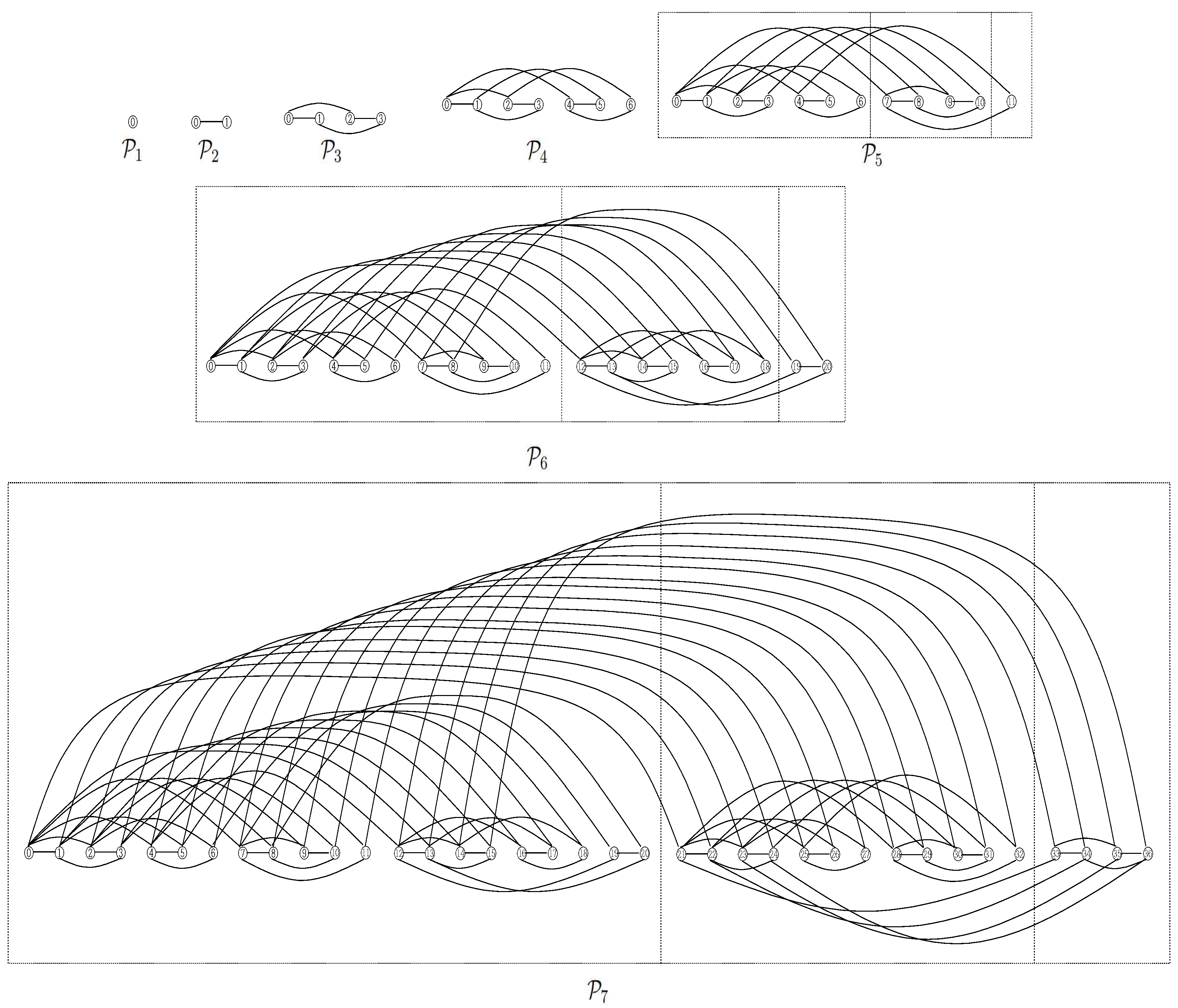
We determine the cube polynomial of the Padovan cubes and read off the number of induced $Q_n$ in ${\mathcal{P}}_n$. To obtain a feeling, we list the first few of them (see Figure 1): $C({\mathcal{P}}_1,x)=1$, $C({\mathcal{P}}_2,x)=2+x$, $C({\mathcal{P}}_3,x)=4+4x+x^2$, $C({\mathcal{P}}_4,x)=7+9x+3x^2$, $C({\mathcal{P}}_5,x)=12+19x+8x^2+x^3$, $C({\mathcal{P}}_6,x)=21+40x+22x^2+4x^3$.

Now, let us determine the generation function for the sequence of cube polynomials corresponding to the Padovan cube. In the process of obtaining the generation function, we need the Cartesian product for the two graphs. The Cartesian product $G\square H$ of graphs G and H has the vertex set $V\left(G\right)\times V\left(H\right)$, and $\{u,v\}$ is adjacent to $\{u^{\prime },v^{\prime }\}$ if either $u=u^{\prime }$ and $\{v,v^{\prime }\}\in E\left(H\right)$, or $\{u,u^{\prime }\}\in E\left(G\right)$ and $v=v^{\prime }$(see [6]).

Theorem 4.

For the Padovan cube, ${\mathcal{P}}_n$, the generating function of the sequence ${\left\{C({\mathcal{P}}_{n+1},x)\right\}}_{n=0}^{\infty }$ is

$$g(C({\mathcal{P}}_{n+1},x),y)=\sum _{n\ge 0}C({\mathcal{P}}_{n+1},x)y^n=\frac{1+(1+x)y+{(1+x)}^2{y}^2+{(1+x)}^2{y}^3}{1-y-(1+x)y^2-(1+2x)y^4}.$$

Proof. 

Clearly, $C({\mathcal{P}}_1,x)=1$, $C({\mathcal{P}}_2,x)=2+x$, $C({\mathcal{P}}_3,x)=4+4x+x^2$, and $C({\mathcal{P}}_4,x)=7+9x+3x^2$.

Let $n\ge 4$ and let

$$X_n=\{v=b_{n-1}{b}_{n-2}\dots b_1\in V\left({\mathcal{P}}_n\right)|b_{n-1}=0\},$$

$$Y_n=\{v=b_{n-1}{b}_{n-2}\dots b_1\in V\left({\mathcal{P}}_n\right)|b_{n-1}=1,b_{n-2}=0\},$$

and

$$Z_n=\{v=b_{n-1}{b}_{n-2}\dots b_1\in V\left({\mathcal{P}}_n\right)|b_{n-1}=b_{n-2}=1,b_{n-3}=b_{n-4}=0\}.$$

Then, $X_n$ induces a subgraph of ${\mathcal{P}}_n$ isomorphic to ${\mathcal{P}}_{n-1}$. The first two coordinates of a vertex from $Y_n$ are 10; hence, $Y_n$ induces a subgraph of ${\mathcal{P}}_n$ isomorphic to ${\mathcal{P}}_{n-2}$. The first four coordinates of a vertex from $Z_n$ are 1100; hence, $Z_n$ induces a subgraph of ${\mathcal{P}}_n$ isomorphic to ${\mathcal{P}}_{n-4}$. Moreover, every vertex from $Y_n$ has exactly one neighbor in $X_n$ and these edges form a matching, every vertex from $Z_n$ has exactly one neighbor in $X_n$ and these edges form a matching, and every vertex from $Z_n$ has exactly one neighbor in $Y_n$ and these edges form a matching.

Hence, for a subgraph H of ${\mathcal{P}}_n$ isomorphic to $Q_k$, we have exactly one of the following exclusive possibilities: (i) H lies in the subgraph induced by $X_n$, (ii) H lies in the subgraph induced by $Y_n$, (iii) H lies in the subgraph induced by $Z_n$, or (iv) $H=K\square K_2$, where K is isomorphic to $Q_{k-1}$ and the edges of $K\square K_2$ corresponding to $K_2$ are edges between $X_n$ and $Y_n$, $X_n$ and $Z_n$, and $Y_n$ and $Z_n$. It follows that, for $n\ge 4$,

$$\begin{array}{c}\hfill C({\mathcal{P}}_{n+1},x)=C({\mathcal{P}}_n,x)+(1+x)C({\mathcal{P}}_{n-1},x)+(1+2x)C({\mathcal{P}}_{n-3},x).\end{array}$$

Setting $g(C({\mathcal{P}}_{n+1},x),y)={\sum }_{n\ge 0}C({\mathcal{P}}_{n+1},x)y^n$, we have

$$\begin{array}{c}\hfill g(C({\mathcal{P}}_{n+1},x),y)=1+(2+x)y+(4+4x+x^2)y^2+(7+9x+3x^2)y^3+\sum _{n\ge 4}C({\mathcal{P}}_{n+1},x)y^n.\end{array}$$

(7)

In (7),

$$\begin{array}{cc}\hfill \sum _{n\ge 4}C({\mathcal{P}}_{n+1},x)y^n& =y\sum _{n\ge 3}C({\mathcal{P}}_{n+1},x)y^n+(1+x)y^2\sum _{n\ge 2}C({\mathcal{P}}_{n+1},x)y^n\hfill \\ \hfill & +(1+2x)y^4\sum _{n\ge 0}C({\mathcal{P}}_{n+1},x)y^n.\hfill \end{array}$$

Since

$$\begin{array}{cc}\hfill y\sum _{n\ge 3}C({\mathcal{P}}_{n+1},x)y^n& =y(g(C({\mathcal{P}}_{n+1},x),y)-1-(2+x)y-(4+4x+x^2)y^2),\hfill \\ \hfill (1+x)y^2\sum _{n\ge 2}C({\mathcal{P}}_{n+1},x)y^n& =(1+x)y^2(g(C({\mathcal{P}}_{n+1},x),y)-1-(2+x)y),\hfill \end{array}$$

and

$$(1+2x)y^4\sum _{n\ge 0}C({\mathcal{P}}_{n+1},x)y^n=(1+2x)y^{4}g(C({\mathcal{P}}_{n+1},x),y),$$

from (7), we can obtain

$$\begin{array}{cc}\hfill g(C({\mathcal{P}}_{n+1},x),y)& =1+(2+x)y+(4+4x+x^2)y^2+(7+9x+3x^2)y^3\hfill \\ & +y(g(C({\mathcal{P}}_{n+1},x),y)-1-(2+x)y-(4+4x+x^2)y^2)\hfill \\ \hfill & +(1+x)y^2(g(C({\mathcal{P}}_{n+1},x),y)-1-(2+x)y)+(1+2x)y^{4}g(C({\mathcal{P}}_{n+1},x),y).\hfill \end{array}$$

Therefore, we can obtain

$$g(C({\mathcal{P}}_{n+1},x),y)=\sum _{n\ge 0}C({\mathcal{P}}_{n+1},x)y^n=\frac{1+(1+x)y+{(1+x)}^2{y}^2+{(1+x)}^2{y}^3}{1-y-(1+x)y^2-(1+2x)y^4}.$$

□

For example, from Theorem 4, we can obtain $C({\mathcal{P}}_7,x)=24+75x+66x^2+23x^3+2x^4$. That is, we know that $c_0\left({\mathcal{P}}_7\right)=24=\left|V\left({\mathcal{P}}_7\right)\right|$, $c_1\left({\mathcal{P}}_7\right)=75=\left|E\left({\mathcal{P}}_7\right)\right|$, $c_2\left({\mathcal{P}}_7\right)=66$, which is the number of induced $Q_2$, $c_3\left({\mathcal{P}}_7\right)=23$, which is the number of induced $Q_3$, and $c_4\left({\mathcal{P}}_7\right)=2$, which is the number of induced $Q_4$.

$Q_n$ can be represented as the Cartesian product of n copies of $K_2$. Hence the property $C(G\square H,x)=C(G,x)C(H,x)$ immediately implies that for any $n\ge 0$,

$$C(Q_n,x)={(2+x)}^n=\sum _{k=0}^n\left(\genfrac{}{}{0pt}{}{n}{k}\right){(1+x)}^k.$$

Now, we consider the $C({\mathcal{P}}_{n+1},x)$ for Padovan cubes.

Lemma 1.

The power series representation of $\frac{1}{1-y-(1+x)y^2-(1+2x)y^4}$ is

$$\begin{array}{cc}\hfill \frac{1}{1-y-(1+x)y^2-(1+2x)y^4}& =\sum _{n\ge 0}^{}\sum _{k=0}^n\sum _{\gamma =0}^{n-k}\left(\genfrac{}{}{0pt}{}{k}{n-k-2\gamma }\right)\left(\genfrac{}{}{0pt}{}{n-k-2\gamma }{\gamma }\right)\hfill \\ \hfill \times {(1+x)}^{n-k-3\gamma }{(1+2x)}^{\gamma }{y}^n.\end{array}$$

Proof. 

$$\begin{array}{cc}\hfill \frac{1}{1-y-(1+x)y^2-(1+2x)y^4}& =\sum _{\alpha \ge 0}{(y+(1+x)y^2+(1+2x)y^4)}^{\alpha }\hfill \\ \hfill & =\sum _{\alpha \ge 0}\sum _{\beta =0}^{\alpha }\left(\genfrac{}{}{0pt}{}{\alpha }{\beta }\right){((1+x)y+(1+2x)y^3)}^{\beta }{y}^a\hfill \\ \hfill & =\sum _{\alpha \ge 0}\sum _{\beta =0}^{\alpha }\left(\genfrac{}{}{0pt}{}{\alpha }{\beta }\right){\left(1+\left(\frac{1+2x}{1+x}\right)y^2\right)}^{\beta }{(1+x)}^{\beta }{y}^{\alpha +\beta }\hfill \\ \hfill & =\sum _{\alpha \ge 0}\sum _{\beta =0}^{\alpha }\sum _{\gamma =0}^{\beta }\left(\genfrac{}{}{0pt}{}{\alpha }{\beta }\right)\left(\genfrac{}{}{0pt}{}{\beta }{\gamma }\right){(1+x)}^{\beta -\gamma }{(1+2x)}^{\gamma }{y}^{\alpha +\beta +2\gamma }.\hfill \end{array}$$

Set $n=\alpha +\beta +2\gamma$. Then we have

$$\begin{array}{cc}\hfill \frac{1}{1-y-(1+x)y^2-(1+2x)y^4}& =\sum _{\alpha \ge 0}\sum _{\beta =0}^{\alpha }\sum _{\gamma =0}^{\beta }\left(\genfrac{}{}{0pt}{}{\alpha }{\beta }\right)\left(\genfrac{}{}{0pt}{}{\beta }{\gamma }\right){(1+x)}^{\beta -\gamma }{(1+2x)}^{\gamma }{y}^{\alpha +\beta +2\gamma }\hfill \\ \hfill & =\sum _{n\ge 0}\sum _{k=0}^n\sum _{\gamma =0}^{n-k}\left(\genfrac{}{}{0pt}{}{k}{n-k-2\gamma }\right)\left(\genfrac{}{}{0pt}{}{n-k-2\gamma }{\gamma }\right){(1+x)}^{n-k-3\gamma }\hfill \\ \hfill & \times {(1+2x)}^{\gamma }{y}^n.\hfill \end{array}$$

□

Theorem 5.

For nonnegative integer n, let

$$\begin{array}{cc}\hfill R({\mathcal{P}}_{n+1},x)& =\sum _{n\ge 0}\sum _{k=0}^n\sum _{\gamma =0}^{n-k}\left(\genfrac{}{}{0pt}{}{k}{n-k-2\gamma }\right)\left(\genfrac{}{}{0pt}{}{n-k-2\gamma }{\gamma }\right){(1+x)}^{n-k-3\gamma }{(1+2x)}^{\gamma },\hfill \\ \hfill S({\mathcal{P}}_{n+1},x)& =\sum _{n\ge 0}\sum _{k=0}^{n-1}\sum _{\gamma =0}^{n-k-1}\left(\genfrac{}{}{0pt}{}{k}{n-k-2\gamma -1}\right)\left(\genfrac{}{}{0pt}{}{n-k-2\gamma -1}{\gamma }\right){(1+x)}^{n-k-3\gamma }{(1+2x)}^{\gamma },\hfill \\ \hfill T({\mathcal{P}}_{n+1},x)& =\sum _{n\ge 0}\sum _{k=0}^{n-2}\sum _{\gamma =0}^{n-k-2}\left(\genfrac{}{}{0pt}{}{k}{n-k-2\gamma -2}\right)\left(\genfrac{}{}{0pt}{}{n-k-2\gamma -2}{\gamma }\right){(1+x)}^{n-k-3\gamma }{(1+2x)}^{\gamma },\hfill \\ \hfill U({\mathcal{P}}_{n+1},x)& =\sum _{n\ge 0}\sum _{k=0}^{n-3}\sum _{\gamma =0}^{n-k-3}\left(\genfrac{}{}{0pt}{}{k}{n-k-2\gamma -3}\right)\left(\genfrac{}{}{0pt}{}{n-k-2\gamma -3}{\gamma }\right){(1+x)}^{n-k-3\gamma -1}{(1+2x)}^{\gamma }.\hfill \end{array}$$

Then

$$C({\mathcal{P}}_{n+1},x)=R({\mathcal{P}}_{n+1},x)+S({\mathcal{P}}_{n+1},x)+T({\mathcal{P}}_{n+1},x)+U({\mathcal{P}}_{n+1},x).$$

Proof. 

From Theorem 4, we know that

$$\begin{array}{cc}\hfill \sum _{n\ge 0}C({\mathcal{P}}_{n+1},x)y^n& =\frac{1}{1-y-(1+x)y^2-(1+2x)y^4}+\frac{(1+x)y}{1-y-(1+x)y^2-(1+2x)y^4}\hfill \\ \hfill & +\frac{{(1+x)}^2{y}^2}{1-y-(1+x)y^2-(1+2x)y^4}+\frac{{(1+x)}^2{y}^3}{1-y-(1+x)y^2-(1+2x)y^4}.\hfill \end{array}$$

From Lemma 1, we obtain

$$\begin{array}{cc}\hfill \sum _{n\ge 0}C({\mathcal{P}}_{n+1},x)y^n& =\sum _{n\ge 0}\left(\sum _{k=0}^n\sum _{\gamma =0}^{n-k}\left(\genfrac{}{}{0pt}{}{k}{n-k-2\gamma }\right)\left(\genfrac{}{}{0pt}{}{n-k-2\gamma }{\gamma }\right){(1+x)}^{n-k-3\gamma }{(1+2x)}^{\gamma }\right.\hfill \\ \hfill & +\sum _{k=0}^{n-1}\sum _{\gamma =0}^{n-k-1}\left(\genfrac{}{}{0pt}{}{k}{n-k-2\gamma -1}\right)\left(\genfrac{}{}{0pt}{}{n-k-2\gamma -1}{\gamma }\right){(1+x)}^{n-k-3\gamma }{(1+2x)}^{\gamma }\hfill \\ \hfill & +\sum _{k=0}^{n-2}\sum _{\gamma =0}^{n-k-2}\left(\genfrac{}{}{0pt}{}{k}{n-k-2\gamma -2}\right)\left(\genfrac{}{}{0pt}{}{n-k-2\gamma -2}{\gamma }\right){(1+x)}^{n-k-3\gamma }{(1+2x)}^{\gamma }\hfill \\ \hfill & \left.+\sum _{k=0}^{n-3}\sum _{\gamma =0}^{n-k-3}\left(\genfrac{}{}{0pt}{}{k}{n-k-2\gamma -3}\right)\left(\genfrac{}{}{0pt}{}{n-k-2\gamma -3}{\gamma }\right){(1+x)}^{n-k-3\gamma -1}{(1+2x)}^{\gamma }\right)y^n.\hfill \end{array}$$

Therefore, we can obtain $C({\mathcal{P}}_{n+1},x)=R({\mathcal{P}}_{n+1},x)+S({\mathcal{P}}_{n+1},x)+T({\mathcal{P}}_{n+1},x)+$$U({\mathcal{P}}_{n+1},x)$. □

For example, from Theorem 5, we can obtain $C({\mathcal{P}}_6,x)=21+40x+22x^2+4x^3$ and $C({\mathcal{P}}_7,x)=24+75x+66x^2+23x^3+2x^4$.

Recall that, for the odd-Padovan sequence $\left\{a_n\right\}$, $a_1=1$, $a_2=2$, $a_3=4$, $a_4=7$, and for $n\ge 5$, $a_n=a_{n-1}+a_{n-2}+a_{n-4}$. Now we consider the generating function of the odd-Padovan sequence.

Lemma 2.

The generating function of the odd-Padovan sequence $\left\{a_n\right\}$ is

$$g(\left\{a_n\right\},y)=\frac{1+y+y^2+y^3}{1-y-y^2-y^4}.$$

Proof. 

Since $a_1=1$, $a_2=2$, $a_3=4$, $a_4=7$, and for $n\ge 5$, $a_n=a_{n-1}+a_{n-2}+a_{n-4}$, we have

$$\begin{array}{c}\hfill g(\left\{a_n\right\},y)=\sum _{n\ge 0}^{}{a}_{n+1}{y}^n=1+2y+4y^2+7y^3+y^4\sum _{n\ge 4}{a}_{n+1}{y}^{n-4}.\end{array}$$

(8)

In (8),

$$\begin{array}{cc}\hfill y^4\sum _{n\ge 4}{a}_{n+1}{y}^{n-4}& =y\sum _{n\ge 3}{a}_{n+1}{y}^n+y^2\sum _{n\ge 2}{a}_{n+1}{y}^n+y^4\sum _{n\ge 0}{a}_{n+1}{y}^n\hfill \\ \hfill & =y(g(\left\{a_n\right\},y)-a_1-a_{2}y-a_3{y}^2)+y^2(g(\left\{a_n\right\},y)-a_1-a_{2}y)+y^{4}g(\left\{a_n\right\},y).\hfill \end{array}$$

Therefore, we can obtain

$$g(\left\{a_n\right\},y)=(y+y^2+y^4)g(\left\{a_n\right\},y)+1+y+y^2+y^3.$$

Therefore, the proof is completed. □

Recall that the $c_n\left(G\right)$ is the number of induced subgraphs of G isomorphic to $Q_n$ for $n\ge 0$. We next determine, for a fixed k, the generating function of the sequence ${\left\{c_k\left({\mathcal{P}}_{n+1}\right)\right\}}_{n=0}^{\infty }$:

Theorem 6.

For a fixed integer $k\ge 0$, let $g(c_k\left({\mathcal{P}}_{n+1}\right),y)={\sum }_{n\ge 0}{c}_k\left({\mathcal{P}}_{n+1}\right)y^n$. And let $\delta \left(y\right)=y^2(1+y)(1-y+3y^3+y^4+2y^6+y^8)$. Then we have

$$\begin{array}{c}\hfill g(c_0\left({\mathcal{P}}_{n+1}\right),y)=\frac{1+y+y^2+y^3}{1-y-y^2-y^4},g(c_1\left({\mathcal{P}}_{n+1}\right),y)=\frac{y+2y^2-y^4}{{(1-y-y^2-y^4)}^2},\end{array}$$

and, for $n\ge 2$ and $k\ge 2$,

$$g(c_k\left({\mathcal{P}}_{n+1}\right),y)=\sum _{n\ge 0}^{}{c}_k\left({\mathcal{P}}_{n+1}\right)y^n=\frac{{(y^2+2y^4)}^{k-2}\delta \left(y\right)}{{(1-y-y^2-y^4)}^{k+1}}.$$

Proof. 

Since $c_0\left({\mathcal{P}}_{n+1}\right)=\left|V\left({\mathcal{P}}_{n+1}\right)\right|=a_{n+1}$, from Lemma 2, we have

$$g(c_0\left({\mathcal{P}}_{n+1}\right),y)=\frac{1+y+y^2+y^3}{1-y-y^2-y^4}.$$

As in the proof of Theorem 4, let $n\ge 4$ and consider the partition of $V\left({\mathcal{P}}_n\right)$ into the sets $X_n=\{v=b_{n-1}{b}_{n-2}\dots b_1\in V\left({\mathcal{P}}_n\right)|b_{n-1}=0\}$, $Y_n=\{v=b_{n-1}{b}_{n-2}\dots b_1\in V\left({\mathcal{P}}_n\right)|b_{n-1}=1,b_{n-2}=0\}$, and $Z_n=\{v=b_{n-1}{b}_{n-2}\dots b_1\in V\left({\mathcal{P}}_n\right)|b_{n-1}=b_{n-2}=1,b_{n-3}=b_{n-4}=0\}$. Then a subgraph H of ${\mathcal{P}}_n$ isomorphic to $Q_k$ either lies in the subgraph induced by $X_n$, it lies in the subgraph induced by $Y_n$, it lies in the subgraph induced by $Z_n$, or it is of the form $K\square K_2$ with $K=Q_{k-1}$ and the edges of $K\square K_2$ corresponding to $K_2$ are edges between $X_n$ and $Y_n$, $X_n$ and $Z_n$, and $Y_n$ and $Z_n$. Thus we have, for $n\ge 4$,

$$\begin{array}{c}\hfill c_k\left({\mathcal{P}}_{n+1}\right)=c_k\left({\mathcal{P}}_n\right)+c_k\left({\mathcal{P}}_{n-1}\right)+c_k\left({\mathcal{P}}_{n-3}\right)+c_{k-1}\left({\mathcal{P}}_{n-1}\right)+2c_{k-1}\left({\mathcal{P}}_{n-3}\right).\end{array}$$

(9)

Note that $c_0\left({\mathcal{P}}_1\right)=a_1=1$, $c_0\left({\mathcal{P}}_2\right)=a_2=2$, $c_0\left({\mathcal{P}}_3\right)=a_3=4$, $c_0\left({\mathcal{P}}_4\right)=a_4=7$, $c_1\left({\mathcal{P}}_1\right)=0$, $c_1\left({\mathcal{P}}_2\right)=1$, $c_1\left({\mathcal{P}}_3\right)=4$, $c_1\left({\mathcal{P}}_4\right)=9$, and

$$\begin{array}{c}\hfill g(c_1\left({\mathcal{P}}_{n+1}\right),y)=\sum _{n\ge 0}^{}{c}_1\left({\mathcal{P}}_{n+1}\right)y^n=y+4y^2+9y^3+\sum _{n\ge 4}{c}_1\left({\mathcal{P}}_{n+1}\right)y^n.\end{array}$$

(10)

In (10), we have, from (9),

$$\begin{array}{cc}\hfill \sum _{n\ge 4}{c}_1\left({\mathcal{P}}_{n+1}\right)y^n& =y\sum _{n\ge 3}{c}_1\left({\mathcal{P}}_{n+1}\right)y^n+y^2\sum _{n\ge 2}{c}_1\left({\mathcal{P}}_{n+1}\right)y^n+y^{4}g(c_1\left({\mathcal{P}}_{n+1}\right),y)\hfill \\ \hfill & +y^2\sum _{n\ge 2}{c}_0\left({\mathcal{P}}_{n+1}\right)y^n+2y^{4}g(c_0\left({\mathcal{P}}_{n+1}\right),y)\hfill \\ \hfill & =y(g(c_1\left({\mathcal{P}}_{n+1}\right),y)-c_1\left({\mathcal{P}}_1\right)-c_1\left({\mathcal{P}}_2\right)y-c_1\left({\mathcal{P}}_3\right)y^2)\hfill \\ \hfill & +y^2(g(c_1\left({\mathcal{P}}_{n+1}\right),y)-c_1\left({\mathcal{P}}_1\right)-c_1\left({\mathcal{P}}_2\right)y)+y^{4}g(c_1\left({\mathcal{P}}_{n+1}\right),y)\hfill \\ \hfill & +y^2(g(c_0\left({\mathcal{P}}_{n+1}\right),y)-c_0\left({\mathcal{P}}_0\right)-c_1\left({\mathcal{P}}_2\right)y)+2y^{4}g(c_0\left({\mathcal{P}}_{n+1}\right),y)\hfill \\ \hfill & =(y+y^2+y^4)g(c_1\left({\mathcal{P}}_{n+1}\right),y)-2y^2-7y^3+(y^2+2y^4)g(c_0\left({\mathcal{P}}_{n+1}\right),y).\hfill \end{array}$$

Therefore, we have

$$\begin{array}{cc}\hfill g(c_1\left({\mathcal{P}}_{n+1}\right),y)& =y+4y^2+9y^3+(y+y^2+y^4)g(c_1\left({\mathcal{P}}_{n+1}\right),y)-2y^2-7y^3\hfill \\ \hfill & +(y^2+2y^4)g(c_0\left({\mathcal{P}}_{n+1}\right),y).\hfill \end{array}$$

Since $g(c_0\left({\mathcal{P}}_{n+1}\right),y)=\frac{1+y+y^2+y^3}{1-y-y^2-y^4}$, we can obtain

$$g(c_1\left({\mathcal{P}}_{n+1}\right),y)=\frac{y+2y^2-y^4}{{(1-y-y^2-y^4)}^2}.$$

Since $c_2\left({\mathcal{P}}_1\right)=c_2\left({\mathcal{P}}_2\right)=0$, $c_2\left({\mathcal{P}}_3\right)=1$, and $c_2\left({\mathcal{P}}_4\right)=3$, a routine computation yields

$$g(c_2\left({\mathcal{P}}_{n+1}\right),y)=\frac{\delta \left(y\right)}{{(1-y-y^2-y^4)}^3},$$

where $\delta \left(y\right)=y^2(1+y)(1-y+3y^3+y^4+2y^6+y^8)$. Also, since $c_3\left({\mathcal{P}}_1\right)=c_3\left({\mathcal{P}}_2\right)=c_3\left({\mathcal{P}}_3\right)=c_3\left({\mathcal{P}}_4\right)=0$, a routine computation yields

$$g(c_3\left({\mathcal{P}}_{n+1}\right),y)=\frac{(y^2+2y^4)\delta \left(y\right)}{{(1-y-y^2-y^4)}^4}.$$

By induction on $k\ge 3$, we can obtain

$$g(c_k\left({\mathcal{P}}_{n+1}\right),y)=\frac{{(y^2+2y^4)}^{k-2}\delta \left(y\right)}{{(1-y-y^2-y^4)}^{k+1}}.$$

Therefore, the proof is completed. □

Now, we define a sequence $\left\{r_n\right\}$ of positive integers by using the odd-Padovan sequence $\left\{a_n\right\}$. Let $\left\{r_n\right\}$ be defined as following; $r_0=a_1$, $r_1=a_1$, $r_2=a_2$, $r_3=a_1+a_2$, $r_4=a_2+a_3$, and for $n\ge 5$, $r_n=r_{n-1}+r_{n-2}+r_{n-4}$. The first few values of $r_n$ are $1,1,2,3,6,10,18,31,55,96,169,296,\dots$.

Lemma 3.

The generating function of the sequence $\left\{r_n\right\}$ is

$$g(\left\{r_n\right\},y)=\frac{1}{1-y-y^2-y^4}.$$

Proof. 

Since

$$g(\left\{r_n\right\},y)=1+y+2y^2+3y^3+6y^4+y^5\sum _{n\ge 5}{r}_n{y}^{n-5},$$

and, for $n\ge 4$, $r_n=r_{n-1}+r_{n-2}+r_{n-4}$, we have

$$g(\left\{r_n\right\},y)=\frac{1}{1-y-y^2-y^4}.$$

□

Lemma 4.

For the sequence $\left\{r_n\right\}$,

$$r_n=\sum _{k=0}^n\sum _{\gamma =0}^{n-k}\left(\genfrac{}{}{0pt}{}{k}{n-k-2\gamma }\right)\left(\genfrac{}{}{0pt}{}{n-k-2\gamma }{\gamma }\right).$$

That is,

$$g(\left\{r_n\right\},y)=\sum _{n\ge 0}^{}\left(\sum _{k=0}^n\sum _{\gamma =0}^{n-k}\left(\genfrac{}{}{0pt}{}{k}{n-k-2\gamma }\right)\left(\genfrac{}{}{0pt}{}{n-k-2\gamma }{\gamma }\right)\right)y^n.$$

Proof. 

Since

$$\sum _{n\ge 0}{r}_n{y}^n=\sum _{\alpha \ge 0}{(1+y+y^3)}^{\alpha }{y}^{\alpha },$$

we have

$$\begin{array}{cc}\hfill \sum _{\alpha \ge 0}{(1+y+y^3)}^{\alpha }{y}^{\alpha }& =\sum _{\alpha \ge 0}\sum _{\beta =0}^{\alpha }\left(\genfrac{}{}{0pt}{}{\alpha }{\beta }\right){(1+y^2)}^{\beta }{y}^{\alpha +\beta }\hfill \\ \hfill & =\sum _{\alpha \ge 0}\sum _{\beta =0}^{\alpha }\sum _{\gamma =0}^{\beta }\left(\genfrac{}{}{0pt}{}{\alpha }{\beta }\right)\left(\genfrac{}{}{0pt}{}{\beta }{\gamma }\right)y^{\alpha +\beta +2\gamma }.\hfill \end{array}$$

(11)

Set $n=\alpha +\beta +2\gamma$. Then $\beta =n-\alpha -2\gamma$, and hence, if $\beta =0$, then $n=\alpha +2\gamma$. So, from (11), we can obtain

$$\begin{array}{c}\hfill g(\left\{r_n\right\},y)=\sum _{n\ge 0}\sum _{k=0}^n\sum _{\gamma =0}^{n-k}\left(\genfrac{}{}{0pt}{}{k}{n-k-2\gamma }\right)\left(\genfrac{}{}{0pt}{}{n-k-2\gamma }{\gamma }\right)y^n.\end{array}$$

Therefore, the proof is completed. □

Corollary 2.

For nonnegative integer n, k,

$$\begin{array}{cc}\hfill \sum _{k=0}^{2n+2}\left(\genfrac{}{}{0pt}{}{k+1}{2n-2k+2}\right)& =\sum _{k=0}^n\sum _{\gamma =0}^{n-k}\left(\genfrac{}{}{0pt}{}{k}{n-k-2\gamma }\right)\left(\genfrac{}{}{0pt}{}{n-k-2\gamma }{\gamma }\right)\hfill \\ \hfill & +\sum _{k=0}^{n-1}\sum _{\gamma =0}^{n-k-1}\left(\genfrac{}{}{0pt}{}{k}{n-k-2\gamma -1}\right)\left(\genfrac{}{}{0pt}{}{n-k-2\gamma -1}{\gamma }\right)\hfill \\ \hfill & +\sum _{k=0}^{n-2}\sum _{\gamma =0}^{n-k-2}\left(\genfrac{}{}{0pt}{}{k}{n-k-2\gamma -2}\right)\left(\genfrac{}{}{0pt}{}{n-k-2\gamma -2}{\gamma }\right)\hfill \\ \hfill & +\sum _{k=0}^{n-3}\sum _{\gamma =0}^{n-k-3}\left(\genfrac{}{}{0pt}{}{k}{n-k-2\gamma -3}\right)\left(\genfrac{}{}{0pt}{}{n-k-2\gamma -3}{\gamma }\right).\hfill \end{array}$$

Proof. 

From Lemma 4, we have, for $i\ge 0$,

$$\frac{y^i}{1-y-y^2-y^4}=\sum _{n\ge 0}\sum _{k=0}^{n-i}\sum _{\gamma =0}^{n-k-i}\left(\genfrac{}{}{0pt}{}{k}{n-k-2\gamma -i}\right)\left(\genfrac{}{}{0pt}{}{n-k-2\gamma -i}{\gamma }\right)y^n.$$

And, from Theorem 6, we have

$$\sum _{n\ge 0}{a}_{n+1}{y}^n=\frac{1+y+y^2+y^3}{1-y-y^2-y^4}.$$

Since $a_{n+1}=P_{2n+3}={\sum }_{k=0}^{2n+2}\left(\genfrac{}{}{0pt}{}{k+1}{2n-2k+2}\right)$, we can obtain the conclusion. □

Lee and Kim [10] gave the number of edges of the Padovan cube ${\mathcal{P}}_n$ as follows, for $n\ge 4$,

$$ϵ\left({\mathcal{P}}_{n+1}\right)=ϵ\left({\mathcal{P}}_n\right)+ϵ\left({\mathcal{P}}_{n-1}\right)+ϵ\left({\mathcal{P}}_{n-3}\right)+a_{n-1}+2a_{n-3},$$

where $ϵ\left({\mathcal{P}}_n\right)$ is the number of edges of the Padovan cube ${\mathcal{P}}_n$. In this paper, we give the number of edges of the Padovan cube ${\mathcal{P}}_n$. To do this, we first introduce the convolution of the two sequences. Let ${\left\{A_n\right\}}_{n=0}^{\infty }$ and ${\left\{B_n\right\}}_{n=0}^{\infty }$ be two sequences of numbers, then the convolution of $A_n$ and $B_n$ is the sequence ${\left\{{(A\ast B)}_n\right\}}_{n=0}^{\infty }$ defined by ${(A\ast B)}_n={\sum }_{i=0}^n{A}_i{B}_{n-i}$ (see [6]). From the definition, it is clear that the generating function of ${\left\{{(A\ast B)}_n\right\}}_{n=0}^{\infty }$ is the product of those of ${\left\{A_n\right\}}_{n=0}^{\infty }$ and ${\left\{B_n\right\}}_{n=0}^{\infty }$ We will denote by $A^{\ast m}$ the sequence defined by $A^{\ast 1}=A$ and $A^{\ast m}=A\ast A^{\ast (m-1)}$, $m\ge 2$.

Theorem 7.

The number of edges of the Padovan cube ${\mathcal{P}}_{n+1}$ is, for $n\ge 4$,

$$c_1\left({\mathcal{P}}_{n+1}\right)=r_{n-1}^{\ast 2}+2r_{n-2}^{\ast 2}-r_{n-4}^{\ast 2},$$

where $r_k^{\ast 2}={\sum }_{i=0}^k{r}_i{r}_{k-i}$ for $k\ge 0$.

Proof. 

Note that $c_1\left({\mathcal{P}}_{n+1}\right)=\left|E\left({\mathcal{P}}_{n+1}\right)\right|$. Since $g(\left\{r_n\right\},y)=\frac{1}{1-y-y^2-y^4}$, we have

$$\sum _{n=0}^{\infty }{r}_n^{\ast 2}{y}^n=\frac{1}{{(1-y-y^2-y^4)}^2}.$$

Thus, the coefficient at $y^n$ in the expansion of $\frac{1}{{(1-y-y^2-y^4)}^2}$ is $r_n^{\ast 2}$ and the coefficient at $y^n$ in the expansion of $\frac{y^k}{{(1-y-y^2-y^4)}^2}$ is $r_{n-k}^{\ast 2}$. From Theorem 6, we know that

$$g\left(c_1({\mathcal{P}}_{n+1},y)\right)=\frac{y+2y^2-y^4}{{(1-y-y^2-y^4)}^2}.$$

Thus, the coefficient at $y^n$ in the expansion of $\frac{y+2y^2-y^4}{{(1-y-y^2-y^4)}^2}$ is $c_1\left({\mathcal{P}}_{n+1}\right)=r_{n-1}^{\ast 2}+2r_{n-2}^{\ast 2}-r_{n-4}^{\ast 2}$. □

4. Lucas–Padovan Cube Polynomial

In this section, we determine the cube polynomial of Ludovan cubes and read off the number of induced $Q_k$ in ${\mathcal{L}}_n$. First, let us determine the generation function of the sequence of cube polynomials corresponding to the Ludovan cube.

Definition 2. [Ludovan cube]

For the nth odd-Ludovan number $l_n$, let N denote an integer, where $1\le N\le l_n$ for some n. Let $I_L$ and $J_L$ denote the Ludovan codes of i and j, $0\le i,j\le N-1$. The Ludovan cube of size N is a graph $\left(V\right(N),E(N\left)\right)$ where $V\left(N\right)=\{0,1,2,\dots ,N-1\}$ and $\{i,j\}\in E\left(N\right)$ if and only if $H(I_P,J_P)=1$.

The Ludovan cube of order n, denoted by ${\mathcal{L}}_n$, is a Ludovan cube with $l_n$ vertices. Define ${\mathcal{L}}_0=(\varnothing ,\varnothing )$.

In [11], the authors gave the following theorem for a characterization of the Ludovan cubes ${\mathcal{L}}_n$.

Theorem 8.

For $n\ge 7$, the Ludovan cube ${\mathcal{L}}_n$ can be decomposed into ${\mathcal{L}}_{n-1}$, ${\mathcal{L}}_{n-2}$, and ${\mathcal{L}}_{n-4}$; the three subgraphs are pairwise disjoint.

For convenience, we consider the empty string and set ${\mathcal{L}}_1=K_1$.

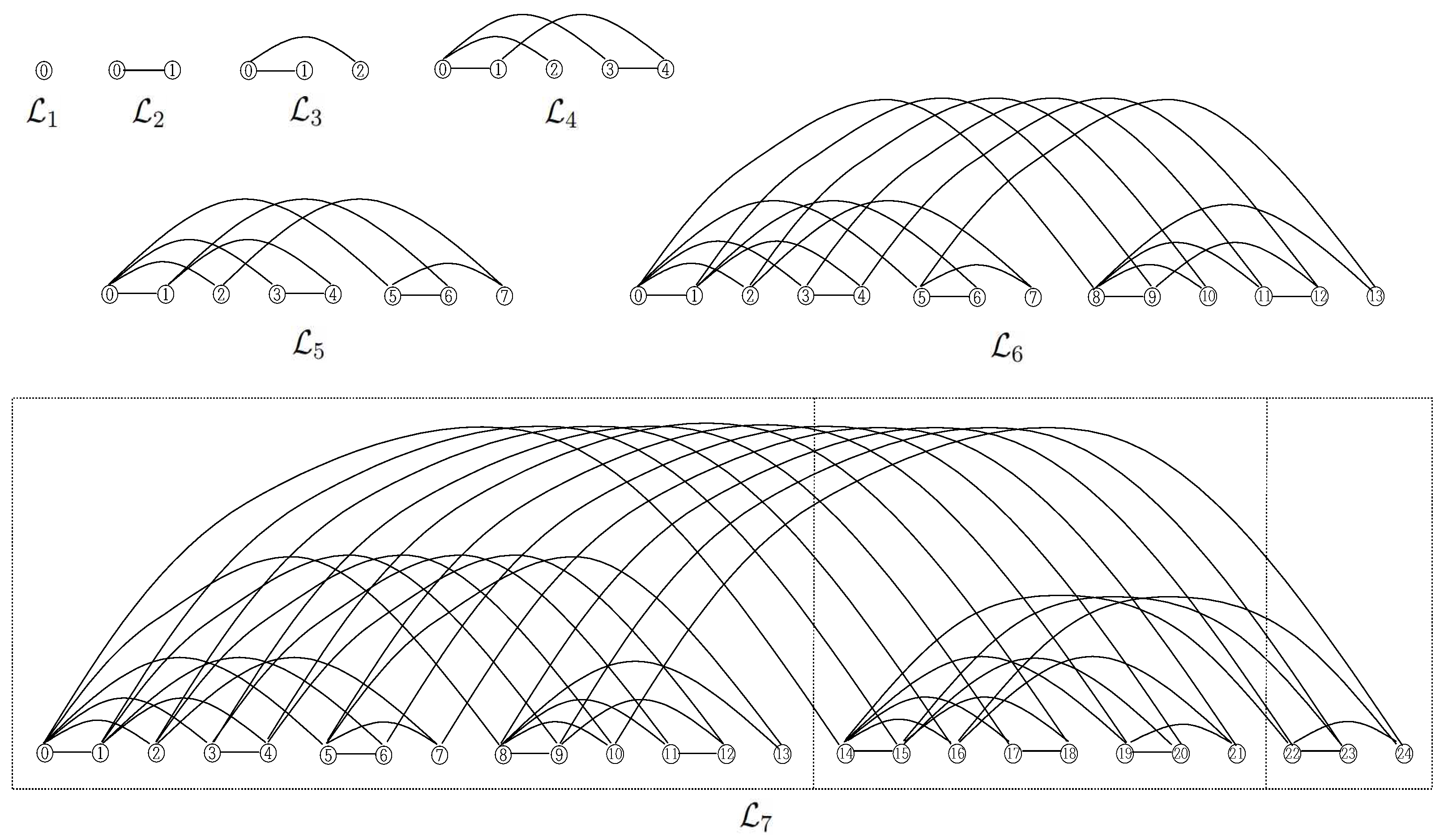
We determine the cube polynomial of the Ludovan cubes and read off the number of induced $Q_n$ in ${\mathcal{L}}_n$. To obtain a feeling, we list the first few of them (see Figure 2): $C({\mathcal{L}}_1,x)=1$, $C({\mathcal{L}}_2,x)=2+x$, $C({\mathcal{L}}_3,x)=3+2x$, $C({\mathcal{L}}_4,x)=5+5x+x^2$, $C({\mathcal{L}}_5,x)=8+10x+3x^2$, $C({\mathcal{L}}_6,x)=14+22x+9x^2+x^3$.

Theorem 9.

For the Ludovan cube ${\mathcal{L}}_n$, the generating function of the sequence ${\left\{C({\mathcal{L}}_{n+1},x)\right\}}_{n=0}^{\infty }$ is

$$\sum _{n\ge 0}C({\mathcal{L}}_{n+1},x)y^n=\frac{1+(1+x)y-(1+2x)y^4-(1+3x+2x^2)y^5}{1-y-(1+x)y^2-(1+2x)y^4}.$$

Proof. 

Clearly, $C({\mathcal{L}}_1,x)=1$, $C({\mathcal{L}}_2,x)=2+x$, $C({\mathcal{L}}_3,x)=3+2x$, $C({\mathcal{L}}_4,x)=5+5x+x^2$, $C({\mathcal{L}}_5,x)=8+10x+3x^2$, $C({\mathcal{L}}_6,x)=14+22x+9x^2+x^3$. Let $X_n=\{v=b_{n-1}{b}_{n-2}\dots b_1\in V\left({\mathcal{L}}_n\right)|b_{n-1}=0\}$, $Y_n=\{v=b_{n-1}{b}_{n-2}\dots b_1\in V\left({\mathcal{L}}_n\right)|b_{n-1}=1,b_{n-2}=0\}$, and $Z_n=\{v=b_{n-1}{b}_{n-2}\dots b_1\in V\left({\mathcal{L}}_n\right)|b_{n-1}=b_{n-2}=1,b_{n-3}=b_{n-4}=0\}$ for $n\ge 6$.

Similarly as in the proof of Theorem 4, we can obtain that, for $n\ge 5$,

$$\begin{array}{c}\hfill C({\mathcal{L}}_{n+1},x)=C({\mathcal{L}}_n,x)+(1+x)C({\mathcal{L}}_{n-1},x)+(1+2x)C({\mathcal{L}}_{n-3},x).\end{array}$$

Set $g(C({\mathcal{L}}_{n+1},x),y)={\sum }_{n\ge 0}C({\mathcal{L}}_{n+1},x)y^n$, we have

$$\begin{array}{cc}\hfill g(C({\mathcal{L}}_{n+1},x),y)& =1+(2+x)y+(3+2x)y^2+(5+5x+x^2)y^3+(8+10x+3x^2)y^4\hfill \\ \hfill & +(14+22x+9x^2+x^3)y^5+\sum _{n\ge 6}C({\mathcal{L}}_{n+1},x)y^n.\hfill \end{array}$$

(12)

In (12), we can obtain

$$(1-y-(1+x)y^2-(1+2x)y^4)g(C({\mathcal{L}}_{n+1},x),y)=1+(1+x)y-(1+2x)y^4-(1+3x+2x^2)y^5.$$

Therefore, we obtain

$$g(C({\mathcal{L}}_{n+1},x),y)=\frac{1+(1+x)y-(1+2x)y^4-(1+3x+2x^2)y^5}{1-y-(1+x)y^2-(1+2x)y^4}.$$

□

For example, from Theorem 9, we can obtain $C({\mathcal{L}}_7,x)=25+48x+26x^2+4x^3$. That is, we know that $c_0\left({\mathcal{L}}_7\right)=25=\left|V\left({\mathcal{L}}_7\right)\right|$, $c_1\left({\mathcal{L}}_7\right)=48=\left|E\left({\mathcal{L}}_7\right)\right|$, $c_2\left({\mathcal{L}}_7\right)=26$, which is the number of induced $Q_2$, and $c_3\left({\mathcal{L}}_7\right)=4$, which is the number of induced $Q_3$.

Theorem 10.

For nonnegative integer n, let

$$\begin{array}{cc}\hfill R^{\prime }({\mathcal{L}}_{n+1},x)& =\sum _{n\ge 0}\sum _{k=0}^n\sum _{\gamma =0}^{n-k}\left(\genfrac{}{}{0pt}{}{k}{n-k-2\gamma }\right)\left(\genfrac{}{}{0pt}{}{n-k-2\gamma }{\gamma }\right){(1+x)}^{n-k-3\gamma }{(1+2x)}^{\gamma },\hfill \\ \hfill S^{\prime }({\mathcal{L}}_{n+1},x)& =\sum _{n\ge 0}\sum _{k=0}^{n-1}\sum _{\gamma =0}^{n-k-1}\left(\genfrac{}{}{0pt}{}{k}{n-k-2\gamma -1}\right)\left(\genfrac{}{}{0pt}{}{n-k-2\gamma -1}{\gamma }\right){(1+x)}^{n-k-3\gamma }{(1+2x)}^{\gamma },\hfill \\ \hfill T^{\prime }({\mathcal{L}}_{n+1},x)& =\sum _{n\ge 0}\sum _{k=0}^{n-4}\sum _{\gamma =0}^{n-k-4}\left(\genfrac{}{}{0pt}{}{k}{n-k-2\gamma -4}\right)\left(\genfrac{}{}{0pt}{}{n-k-2\gamma -4}{\gamma }\right){(1+x)}^{n-k-3\gamma -4}{(1+2x)}^{\gamma +1},\hfill \\ \hfill U^{\prime }({\mathcal{L}}_{n+1},x)& =\sum _{n\ge 0}\sum _{k=0}^{n-5}\sum _{\gamma =0}^{n-k-5}\left(\genfrac{}{}{0pt}{}{k}{n-k-2\gamma -5}\right)\left(\genfrac{}{}{0pt}{}{n-k-2\gamma -5}{\gamma }\right){(1+x)}^{n-k-3\gamma -5}\hfill \\ \hfill & \times {(1+2x)}^{\gamma }(1+3x+2x^2).\hfill \end{array}$$

Then

$$C({\mathcal{L}}_{n+1},x)=R^{\prime }({\mathcal{L}}_{n+1},x)+S^{\prime }({\mathcal{L}}_{n+1},x)+T^{\prime }({\mathcal{L}}_{n+1},x)+U^{\prime }({\mathcal{L}}_{n+1},x).$$

Proof. 

From Theorem 9, we know that

$$\sum _{n\ge 0}C({\mathcal{L}}_{n+1},x)y^n=\frac{1+(1+x)y-(1+2x)y^4-(1+3x+2x^2)y^5}{1-y-(1+x)y^2-(1+2x)y^4}.$$

As in the proof of Theorem 5, we can obtain $C({\mathcal{L}}_{n+1},x)=R^{\prime }({\mathcal{L}}_{n+1},x)+S^{\prime }({\mathcal{L}}_{n+1},x)+T^{\prime }({\mathcal{L}}_{n+1},x)+U^{\prime }({\mathcal{L}}_{n+1},x)$. □

For example, from Theorem 10, we have $C({\mathcal{L}}_7,x)=25+48x+26x^2+4x^3$ and $C({\mathcal{L}}_8,x)=44+99x+68x^2+16x^3+x^4$.

Recall that, for the odd-Ludovan sequence $\left\{l_n\right\}$, $l_1=1$, $l_2=2$, $l_3=3$, $l_4=5$, $l_5=8$, $l_6=14$, and for $n\ge 7$, $l_n=l_{n-1}+l_{n-2}+l_{n-4}$. Now, we consider the generating function of the odd-Ludovan sequence $\left\{l_n\right\}$.

Lemma 5.

The generating function of the odd-Ludovan sequence $\left\{l_n\right\}$ is

$$g(\left\{l_n\right\},y)=\frac{1+y-y^4-y^5}{1-y-y^2-y^4}.$$

Proof. 

Since $l_1=1$, $l_2=2$, $l_3=3$, $l_4=5$, $l_5=8$, $l_6=14$, and for $n\ge 6$, $l_{n+1}=l_n+l_{n-1}+l_{n-3}$, we have

$$g(\left\{l_n\right\},y)=1+2y+3y^2+5y^3+8y^4+14y^5+y^6\sum _{n\ge 6}{l}_{n+1}{y}^{n-6}.$$

As in the proof of Lemma 2, we obtain

$$g(\left\{l_n\right\},y)=(y+y^2+y^4)g(\left\{l_n\right\},y)+1+y-y^4-y^5.$$

Therefore, the proof is completed. □

Theorem 11.

For a fixed $k\ge 0$, let $g(c_k\left({\mathcal{L}}_{n+1}\right),y)={\sum }_{n\ge 0}{c}_k\left({\mathcal{L}}_{n+1}\right)y^n$. And let $\theta \left(y\right)=y^3+4y^6+2y^7+4y^9+4y^{10}+y^{11}$. Then, we have

$$\begin{array}{c}\hfill g(c_0\left({\mathcal{L}}_{n+1}\right),y)=\frac{1+y-y^4-y^5}{1-y-y^2-y^4},g(c_1\left({\mathcal{L}}_{n+1}\right),y)=\sum _{n\ge 0}{c}_1\left({\mathcal{L}}_{n+1}\right)y^n=\frac{y+4y^6+2y^7+y^9}{{(1-y-y^2-y^4)}^2},\end{array}$$

and, for $k\ge 2$,

$$g(c_k\left({\mathcal{L}}_{n+1}\right),y)=\frac{{(y^2+2y^4)}^{k-2}\theta \left(y\right)}{{(1-y-y^2-y^4)}^{k+1}}.$$

Proof. 

Since $c_0\left({\mathcal{L}}_{n+1}\right)=\left|V\left({\mathcal{L}}_{n+1}\right)\right|=l_{n+1}$, we have, from Lemma 5,

$$g(c_0\left({\mathcal{L}}_{n+1}\right),y)=\frac{1+y-y^4-y^5}{1-y-y^2-y^4}.$$

As in the proof of Theorem 6, for $n\ge 5$, we have

$$\begin{array}{c}\hfill c_k\left({\mathcal{L}}_{n+1}\right)=c_k\left({\mathcal{L}}_n\right)+c_k\left({\mathcal{L}}_{n-1}\right)+c_k\left({\mathcal{L}}_{n-3}\right)+c_{k-1}\left({\mathcal{L}}_{n-1}\right)+2c_{k-1}\left({\mathcal{L}}_{n-3}\right).\end{array}$$

(13)

Since $c_0\left({\mathcal{L}}_1\right)=1$, $c_0\left({\mathcal{L}}_2\right)=2$, $c_0\left({\mathcal{L}}_3\right)=3$, $c_0\left({\mathcal{L}}_4\right)=5$, $c_0\left({\mathcal{L}}_5\right)=8$, $c_0\left({\mathcal{L}}_6\right)=14$, $c_1\left({\mathcal{L}}_1\right)=0$, $c_1\left({\mathcal{L}}_2\right)=1$, $c_1\left({\mathcal{L}}_3\right)=2$, $c_1\left({\mathcal{L}}_4\right)=5$, $c_1\left({\mathcal{L}}_5\right)=10$, $c_1\left({\mathcal{L}}_6\right)=22$, and

$$g(c_1\left({\mathcal{L}}_{n+1}\right),y)=y+2y^2+5y^3+10y^4+22y^5+\sum _{n\ge 6}{c}_1\left({\mathcal{L}}_{n+1}\right)y^n,$$

we can obtain

$$g(c_1\left({\mathcal{L}}_{n+1}\right),y)=(y+y^2+y^4)g(c_1\left({\mathcal{L}}_{n+1}\right),y)+y-2y^4-3y^5+(y^2+2y^4)g(c_0\left({\mathcal{L}}_{n+1}\right),y).$$

Since $g(c_0\left({\mathcal{L}}_{n+1}\right),y)=\frac{1+y-y^4-y^5}{1-y-y^2-y^4}$, we have

$$g(c_1\left({\mathcal{L}}_{n+1}\right),y)=\frac{y+4y^6+2y^7+y^9}{{(1-y-y^2-y^4)}^2}.$$

Since $c_2\left({\mathcal{L}}_1\right)=c_2\left({\mathcal{L}}_2\right)=c_2\left({\mathcal{L}}_3\right)=0$, $c_2\left({\mathcal{L}}_4\right)=1$, $c_2\left({\mathcal{L}}_5\right)=3$, $c_2\left({\mathcal{L}}_6\right)=9$, a routine computation, using (13), yields

$$g(c_2\left({\mathcal{L}}_{n+1}\right),y)=\frac{\theta \left(y\right)}{{(1-y-y^2-y^4)}^3},$$

where $\theta \left(y\right)=y^3+4y^6+2y^7+4y^9+4y^{10}+y^{11}$. Since $c_3\left({\mathcal{L}}_1\right)=c_3\left({\mathcal{L}}_2\right)=c_3\left({\mathcal{L}}_3\right)=c_3\left({\mathcal{L}}_4\right)=c_3\left({\mathcal{L}}_5\right)=0$ and $c_3\left({\mathcal{L}}_6\right)=1$, a routine computation, using (13), yields

$$g(c_3\left({\mathcal{L}}_{n+1}\right),y)=\frac{(y^2+2y^4)\theta \left(y\right)}{{(1-y-y^2-y^4)}^4}.$$

By induction on $k\ge 3$, we can obtain

$$g(c_k\left({\mathcal{L}}_{n+1}\right),y)=\frac{{(y^2+2y^4)}^{k-2}\theta \left(y\right)}{{(1-y-y^2-y^4)}^{k+1}}.$$

Therefore, the proof is completed. □

Corollary 3.

For nonnegative integer n, k,

$$\begin{array}{cc}\hfill \sum _{k=0}^{2n-2}\left(\left(\genfrac{}{}{0pt}{}{k}{2n-2k-2}\right)+2\left(\genfrac{}{}{0pt}{}{k+1}{2n-2k-3}\right)\right)& =\sum _{k=0}^n\sum _{\gamma =0}^{n-k}\left(\genfrac{}{}{0pt}{}{k}{n-k-2\gamma }\right)\left(\genfrac{}{}{0pt}{}{n-k-2\gamma }{\gamma }\right)\hfill \\ \hfill & +\sum _{k=0}^{n-1}\sum _{\gamma =0}^{n-k-1}\left(\genfrac{}{}{0pt}{}{k}{n-k-2\gamma -1}\right)\left(\genfrac{}{}{0pt}{}{n-k-2\gamma -1}{\gamma }\right)\hfill \\ \hfill & -\sum _{k=0}^{n-4}\sum _{\gamma =0}^{n-k-4}\left(\genfrac{}{}{0pt}{}{k}{n-k-2\gamma -4}\right)\left(\genfrac{}{}{0pt}{}{n-k-2\gamma -4}{\gamma }\right)\hfill \\ \hfill & -\sum _{k=0}^{n-5}\sum _{\gamma =0}^{n-k-5}\left(\genfrac{}{}{0pt}{}{k}{n-k-2\gamma -5}\right)\left(\genfrac{}{}{0pt}{}{n-k-2\gamma -5}{\gamma }\right).\hfill \end{array}$$

Proof. 

From Lemma 4, we have, for $i\ge 0$,

$$\frac{y^i}{1-y-y^2-y^4}=\sum _{n\ge 0}\sum _{k=0}^{n-i}\sum _{\gamma =0}^{n-k-i}\left(\genfrac{}{}{0pt}{}{k}{n-k-2\gamma -i}\right)\left(\genfrac{}{}{0pt}{}{n-k-2\gamma -i}{\gamma }\right)y^n,$$

and, from Lemma 5 and Theorem 11, we have

$$\sum _{n\ge 0}{l}_{n+1}{y}^n=\frac{1+y-y^4-y^5}{1-y-y^2-y^4}.$$

Since

$$l_{n+1}=L_{2n-1}=\sum _{k=0}^{2n-2}\left(\left(\genfrac{}{}{0pt}{}{k}{2n-2k-2}\right)+2\left(\genfrac{}{}{0pt}{}{k+1}{2n-2k-3}\right)\right),$$

we can obtain the conclusion. □

Lee and Kim [11] gave the number of edges of the Ludovan cube ${\mathcal{L}}_n$ as follows: for $n\ge 6$, Then

$$ϵ\left({\mathcal{L}}_{n+1}\right)=ϵ\left({\mathcal{L}}_n\right)+ϵ\left({\mathcal{L}}_{n-1}\right)+ϵ\left({\mathcal{L}}_{n-3}\right)+l_{n-1}+2l_{n-3}.$$

where $ϵ\left({\mathcal{L}}_n\right)$ is the number of edges of the Ludovan cube ${\mathcal{L}}_n$. From Theorem 11 and Corollary 3, we can obtain another equation for the number of edges of the Ludovan cube ${\mathcal{L}}_n$.

Theorem 12.

The number of edges of the Ludovan cube ${\mathcal{L}}_{n+1}$ is, for $n\ge 9$,

$$c_1\left({\mathcal{L}}_{n+1}\right)=r_{n-1}^{\ast 2}+4r_{n-6}^{\ast 2}+2r_{n-7}^{\ast 2}+r_{n-9}^{\ast 2},$$

where $r_k^{\ast 2}={\sum }_{i=0}^k{r}_i{r}_{k-i}$.

5. Conclusions

In this paper, we covered how to express Padovan and Lucas–Padovan numbers in terms of binomial coefficients by using generating functions. The main contribution of this paper is to present the cube polynomials of Padovan and Lucas–Padovan cubes and analyze their structural properties. The structure and applications of the Padovan cube and the Lucas–Padovan cube have already been introduced in previous studies [10,11].

By obtaining the polynomial for the Padovan cube, we can know exactly how many hypercubes of each degree exist in the Padovan cube. For the Lucas–Padovan cube, the cube polynomial also tells us exactly how many hypercubes there are. This is a very important step in characterizing the structure of both cubes.

However, since the Padovan and Lucas–Padovan sequences are not simple, the cubes introduced by them are very complex, and the cube polynomials are also very complex. In the future, if we study the properties of Padovan and Lucas–Padovan cubes to find a simpler way to represent them, and from that, we can more accurately determine the casting of these cubes, and they can be used in various fields like binary cubes and Fibonacci cubes.

References

- Brešar, B.; Klavžar, S.; Škrekovski, R. The cube polinomial and its derivatives: The case of median graphs. Electron. Comb. 2003, 10, 11. [Google Scholar] [CrossRef]
- Hsu, W. Fibonacci Cubes—A New Interconnection Topology. IEEE Trans. Parallel Distrib. Syst. 1993, 4, 3–12. [Google Scholar] [CrossRef]
- Brešar, B.; Dorbec, P.; Klavžzar, S.; Mollard, M. Hamming polynomials and their partial derivatives. Eur. J. Comb. 2007, 28, 1156–1162. [Google Scholar] [CrossRef] [Green Version]
- Brešar, B.; Klavžar, S.; Škrekovski, R. Roots of cube polynomials of median graphs. J. Graph Theory 2006, 51, 37–50. [Google Scholar] [CrossRef]
- Eğecioğlu, Ö.; Saygi, E.; Saygi, Z. On the chromatic polynomial and the domination number of k-Fibonacci cubes. Turk. J. Math. 2020, 44, 1813–1823. [Google Scholar] [CrossRef]
- Klavžar, S.; Mollard, M. Cube polynomial of Fibonacci and Lucas cubes. Acta Appl. Math. 2012, 117, 93–105. [Google Scholar] [CrossRef]
- Klavžar, S.; Mollard, M. Wiener index and Hosoya polynomial of Fobonacci and Lucas cubes. MATCH Commun. Math. Comput. Chem. 2012, 68, 311–324. [Google Scholar]
- Zelina, I.; Hajdu-Măcelaru, M.; Ţicală, C. About the cube polynomial of extended Fibonacci cubes. Creat. Math. Inform. 2018, 1, 95–100. [Google Scholar] [CrossRef]
- Saygi, E.; Eğecioğlu, Ö. q-cube enumerator polynomial of Fibonacci cubes. Discret. Appl. Math. 2017, 226, 127–137. [Google Scholar] [CrossRef]
- Lee, G.; Kim, J. On the Padovan Codes and the Padovan Cubes. Symmetry 2023, 15, 266. [Google Scholar] [CrossRef]
- Lee, G.; Kim, J.; Park, K.; Kim, M. On the construction of a new topological network using Lucas-Padovan sequence. J. Internet Comput. Serv. 2023, 24, 27–37. [Google Scholar]
- Voet, C. The Poetics of order: Dom Hans Van der Loan’s numbers. Architecton. Space ARQ 2012, 16, 137–154. [Google Scholar]
- Padova, R. Dom Hans Van Der Laan and the Plastic Number. Nexus IV: Architecture and Mathematics. 2002. Available online: http://www.nexusjournal.com/conferences/N2002-Padovan.html (accessed on 19 June 2023).
- Kritsana, S. Matrices formula for Padovan and Perrin Sequences. IEEE Trans. Parallel Distrib. Syst. 1992, 4, 3–12. [Google Scholar]
- Shannon, A.G.; Anderson, A.F.; Anderson, P.R. The Auxiliary Equation Associated with the Plastic Numbers. Notes Number Theory Discret. 2006, 12, 1–12. [Google Scholar]
- Shannon, A.G.; Anderson, P.G.; Horadam, A.F. Van der Loan numbers. Int. J. Math. Educ. Sci. Technol. 2006, 37, 825–831. [Google Scholar] [CrossRef]
- Lee, G. On the k-generalized Padovan Numbers. Util. Math. 2018, 108, 185–194. [Google Scholar]
- Lee, G. On the Generalized Binet Formulas of the k-Padovan Numbers. Far East J. Math. Sci. 2016, 99, 1487–1504. [Google Scholar] [CrossRef]
- Taşcı, D. On Gaussian Leonardo numbers. Contrib. Math. 2023, 7, 34–40. [Google Scholar]
- Munarini, E.; Cippo, C.P.; Salvi, N.Z. On the Lucas cubes. Fibonacci Q. 2001, 39, 12–21. [Google Scholar]
- Eğecioğlu, Ö.; Saygi, E.; Saygi, Z. The structure of k-Lucas cubes. Hacet. J. Math. Stat. 2021, 50, 754–769. [Google Scholar] [CrossRef]
Figure 1.
Padovan cubes from to .
Figure 2.
Ludovan cubes from to .
Disclaimer/Publisher’s Note: The statements, opinions and data contained in all publications are solely those of the individual author(s) and contributor(s) and not of MDPI and/or the editor(s). MDPI and/or the editor(s) disclaim responsibility for any injury to people or property resulting from any ideas, methods, instructions or products referred to in the content. |
© 2023 by the authors. Licensee MDPI, Basel, Switzerland. This article is an open access article distributed under the terms and conditions of the Creative Commons Attribution (CC BY) license (https://creativecommons.org/licenses/by/4.0/).
Share and Cite
MDPI and ACS Style
Lee, G.; Kim, J. On the Cube Polynomials of Padovan and Lucas–Padovan Cubes. Symmetry 2023, 15, 1389. https://doi.org/10.3390/sym15071389
AMA Style
Lee G, Kim J. On the Cube Polynomials of Padovan and Lucas–Padovan Cubes. Symmetry. 2023; 15(7):1389. https://doi.org/10.3390/sym15071389
Chicago/Turabian StyleLee, Gwangyeon, and Jinsoo Kim. 2023. "On the Cube Polynomials of Padovan and Lucas–Padovan Cubes" Symmetry 15, no. 7: 1389. https://doi.org/10.3390/sym15071389
Note that from the first issue of 2016, this journal uses article numbers instead of page numbers. See further details here.