Newton-like Polynomial-Coded Distributed Computing for Numerical Stability

Abstract

For coded distributed computing (CDC), polynomial code is one prevalent encoding method for CDC (called Poly-CDC). It suffers from poor numerical stability due to the Vandermonde matrix serving as the coefficient matrix which needs to be inverted, and whose condition number increases exponentially with the size of the matrix or equivalently with the number of parallel worker nodes. To improve the numerical stability, especially for large networks, we propose a Newton-like polynomial code (NLPC)-based CDC (NLPC-CDC), with a design dedicated for both matrix–vector and matrix–matrix multiplications. The associated proof of the constructed code possesses a $(n,k)$-symmetrical combination property (CP), where symmetrical means the worker nodes have identical computation volume, CP means the k-symmetrical original computing tasks are encoded into $n(n\ge k)$-symmetrically coded computing tasks, and the arbitrary k resulting from the n-coded computing tasks can recover the intended computing results. Extensive numerical studies verify the significant numerical stability improvement of our proposed NLPC-CDC over Poly-CDC.

1. Introduction

Matrix multiplications (especially large matrix multiplications) are widely adopted in data mining, machine learning, etc. [1]. A single computing node may not be able to handle large or frequent matrix multiplications [2,3,4,5,6]. Due to the development of 5G/6G communication techniques [7] and network virtualizations [8] that provide efficient and reliable data delivery, especially in future 6G communication networks, the strict requirements of a high data rate and computational complexity require frequent processing of large matrices [9,10], and distributed computing (DC) based on partitioning computing tasks could effectively alleviate this problem. By introducing proper redundant computing [11,12], coded distributed computing (CDC) effectively tackles the straggler problem of DC [13,14]. Prevalent CDC designs aims at obtaining the $(n,k)$-symmetrical combination property (CP): k original symmetrical computing tasks are encoded into $n(n\ge k)$-coded computing tasks, and the arbitrary k resulting from the n-coded computing tasks can recover the intended computing results [15], where symmetrical means the worker nodes have identical computation volume. Based on this symmetrical assumption, the worker nodes can be viewed as having identical but independent capabilities, and the design focus of CDC can be directed towards achieving $(n,k)$ CP.

Prevalent encoding methods for CDC are based on polynomial encoding methods [16,17,18], and is therefore called Poly-CDC, where the work in [16] set the fundamental/framework for Poly-CDC, while the work in [17,18] reported variants within this framework. More specifically, the the authors of [16] designed the fundamental encoding coefficients which laid the actual framework, and the authors in [17,18] modified the encoding coefficients within this framework. The drawback lies in poor the numerical stability during the associated decoding stage: The coefficient matrix of the polynomial method is a Vandermonde matrix whose condition number increases exponentially with the size of the matrix [19,20,21], and the decoding process inevitably involves the interpolation of polynomials, eventually evolving into the inversion of the coefficient matrix. Note that the size of the matrix may be large by network slicing techniques [22], and a large condition number means that a small perturbation will cause a larger perturbation after decoding [23,24], thus affecting the robustness of the decoding results. This makes large networks have extremely poor numerical stability.

In order to obtain higher numerical stability, based on Newton-like polynomial code (NLPC), we propose an NLPC-based CDC (NLPC-CDC). This encoding is designed for both matrix–vector and matrix–matrix multiplications. An associated proof that the constructed code possesses a $(n,k)$-symmetrical combination property (CP) is provided. Extensive numerical studies verify that this method improves numerical stability significantly.

Preliminaries are given in Section 2. Afterwards, our proposed NLPC-CDC is elaborated upon in Section 3. Numerical comparisons are executed in Section 4. Finally, conclusions are drawn in Section 5.

2. Preliminaries

We first formulate the matrix–vector and matrix–matrix multiplication within the CDC framework. Afterwards, we briefly describe the Newton interpolation polynomial (NIP) encoding method.

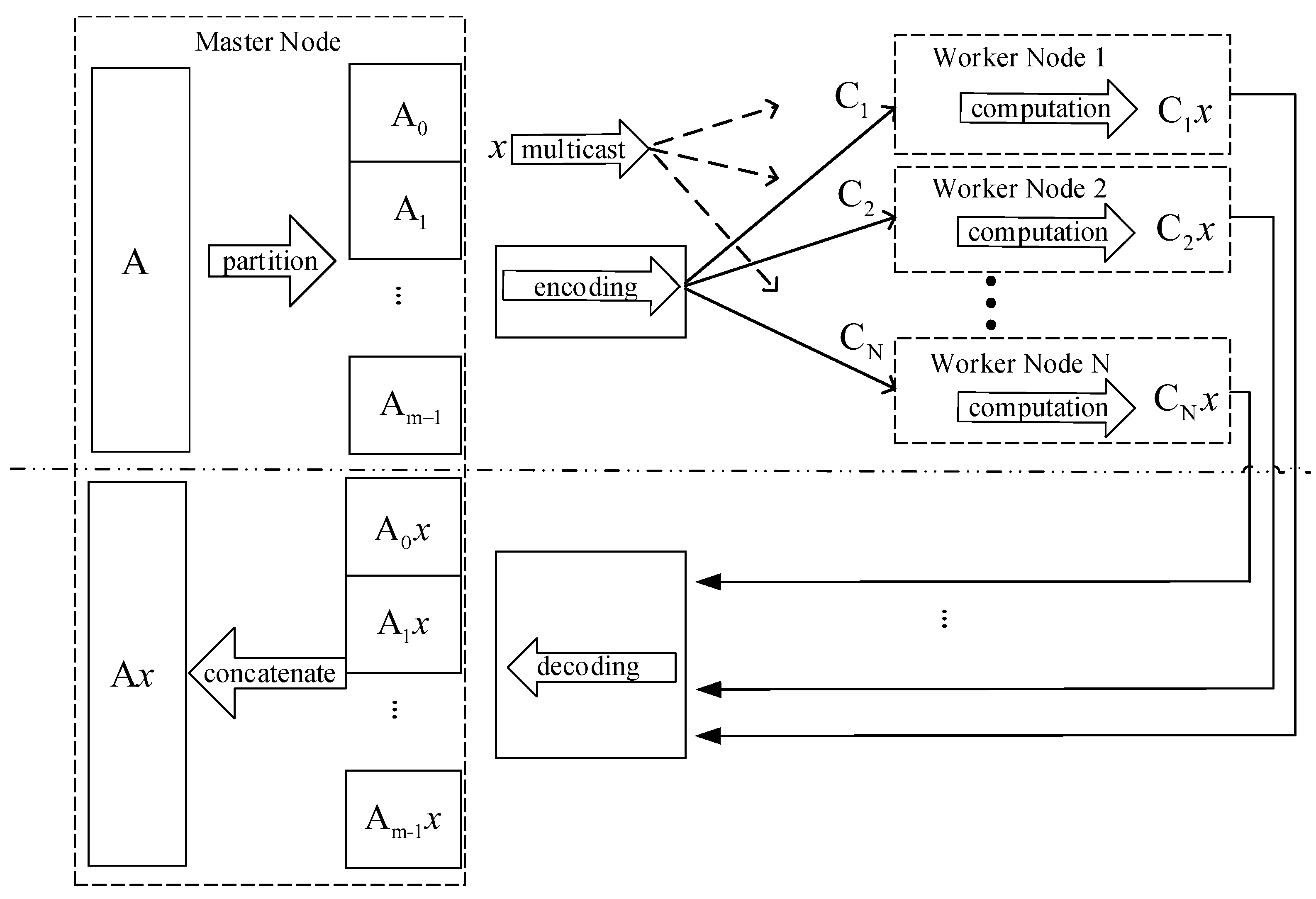
2.1. Matrix–Vector Multiplication within the CDC Framework

The first task is to calculate the matrix–vector multiplication $\mathit{A}\mathit{x}$, where matrix $\mathit{A}\in {\mathrm{R}}^{H\times W}$, column vector $\mathit{x}=\left(x_1,x_2,\dots ,x_W\right)\in {\mathrm{R}}^{W\times 1}$, and $\mathrm{R}$ stands for the real number field. For this task, the computing system consists of a master node and N-symmetrical worker nodes, as shown in Figure 1, where symmetrical means the worker nodes have identical computation capabilities. Under this symmetrical assumption, codes that have symmetical CP can be brought into play to tackle stragglers.

As H is very large, it is necessary to partition matrix $\mathit{A}$ into m sub-matrices, including $A_0\in {\mathrm{R}}^{(H/m)\times W}$ through $A_{m-1}\in {\mathrm{R}}^{(H/m)\times W}$. Encoding the m sub-matrices into N matrices is denoted by $C_1$ through $C_N$.

The master node delivers vector $\mathit{x}$ to all worker nodes. Worker node $i\in \{1,2,\dots ,N\}$ calculates the matrix–vector multiplication $C_i\mathit{x}$ and delivers the calculation result back to the master node. The master node can then execute decoding to recover the intended calculation result provided that enough results have been collected.

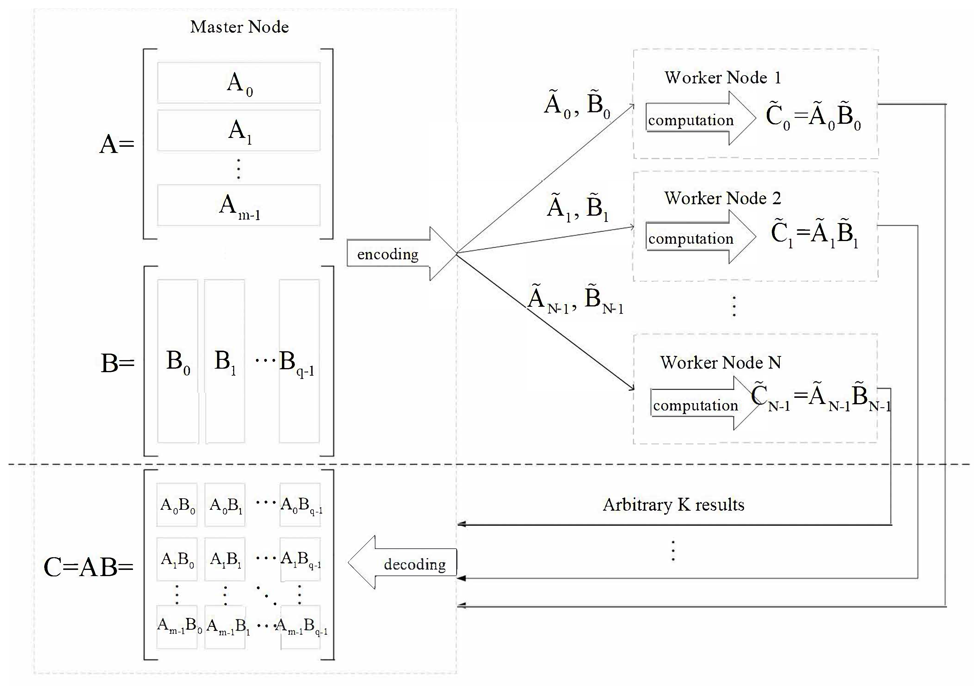
2.2. Matrix–Matrix Multiplication within the CDC Framework

The next task is to calculate the matrix–matrix multiplication $\mathit{A}\mathit{B}$, where the matrix $\mathit{A}\in {\mathrm{R}}^{H\times W}$, $\mathit{B}\in {\mathrm{R}}^{W\times L}$. For this task, the computing system consists of a master node and N worker nodes, as shown in Figure 2. The matrix $\mathit{A}$ is split horizontally into m sub-matrices, including $A_0\in {\mathrm{R}}^{(H/m)\times W}$ through $A_{m-1}\in {\mathrm{R}}^{(H/m)\times W}$. Matrix $\mathit{B}$ is then split vertically into q sub-matrices, including $B_0\in {\mathrm{R}}^{W\times (L/q)}$ through $B_{q-1}\in {\mathrm{R}}^{W\times (L/q)}$. We suppose H and L are divisible by m and q, respectively (otherwise, $\mathit{A}$ and $\mathit{B}$ are filled with zeros so that the number of rows of $\mathit{A}$ and the number of columns of $\mathit{B}$ are multiples of m and q).

The intended calculated matrix $\mathit{C}$ becomes

$$\begin{array}{cc}\hfill \mathit{C}=\mathit{A}\mathit{B}=& \hfill \left[\begin{array}{cccc}{A}_0{B}_0& A_0{B}_1& \cdots & A_0{B}_{q-1}\\ A_1{B}_0& A_1{B}_1& \cdots & A_1{B}_{q-1}\\ ⋮& ⋮& \ddots & ⋮\\ A_{m-1}{B}_0& A_{m-1}{B}_1& \cdots & A_{m-1}{B}_{q-1}\end{array}\right]\\ \hfill \triangleq & \hfill \left[\begin{array}{cccc}{C}_0& C_1& \cdots & C_{q-1}\\ C_q& C_{q+1}& \cdots & C_{2q-1}\\ ⋮& ⋮& \ddots & ⋮\\ C_{(m-1)q}& C_{(m-1)q+1}& \cdots & C_{mq-1}\end{array}\right].\end{array}$$

(1)

Calculating $\mathit{C}$ is equivalent to calculating $C_0$ through $C_{mq-1}$ simultaneously. We set the recovery threshold $K=mq$, directly allocate $C_0$ through $C_{mq-1}$ to K-symmetrical worker nodes (worker node i calculates $C_i$), and the calculation will encounter the problem of stragglers.

To tackle the straggler problem, an encoding strategy is applied on $A_0$ through $A_{m-1}$ to obtain $N>K$-encoded sub-matrices, recorded as ${\tilde{A}}_0$ through ${\tilde{A}}_{N-1}$. Similarly, $B_0$ through $B_{q-1}$ are encoded into ${\tilde{B}}_0$ through ${\tilde{B}}_{N-1}$.

The master node delivers the encoded pair $\left({\tilde{A}}_i,{\tilde{B}}_i\right)$ to worker node $i\in \mathcal{N}\triangleq \{1,2,\dots ,N\}$. Worker node $i\in \mathcal{N}$ then calculates the matrix–matrix multiplication ${\tilde{C}}_i={\tilde{A}}_i{\tilde{B}}_i$ and delivers the calculation result back to the master node, which will then execute decoding to recover the original intended calculation result.

2.3. Newton Interpolation Polynomial (NIP) Encoding

As illustrated previously, symmetrical assumption leads the design to focus on CP encoding that can be directly applied in CDC systems. NIP may serve as a candidate for this encoding design.

NIP improves upon the Lagrange interpolation method by saving the number of multiplication and division operations. In addition, its base is not as complex as the Lagrange function, thus the solving process is much simpler than that of monomial based methods.

We suppose there are $n+1$ real interpolation points $x_0\cdots x_n$ in interval $[a,b]$, and the selected base is

$$\begin{array}{c}\hfill {\pi }_j\left(x\right)=\prod _{k=0}^{j-1}\left(x-x_k\right)=\left(x-x_0\right)\left(x-x_1\right)\cdots \left(x-x_{j-1}\right),\end{array}$$

(2)

for $j=0,1,\dots ,n$. This base has the property ${\pi }_j\left(x_i\right)=0$ for $\forall i<j$.

The polynomial form obtained by linear combination based on ${\pi }_j\left(x\right)$ is

$$\begin{array}{ll}{\displaystyle \sum _{j=0}^n}{a}_j{\pi }_j\left(x\right)=& a_0+a_1\left(x-x_0\right)+a_2\left(x-x_0\right)\left(x-x_1\right)+\cdots \\ & + a_n\left(x-x_0\right)\left(x-x_1\right)\cdots \left(x-x_{n-1}\right),\end{array}$$

(3)

where $a_j$ is the undetermined coefficient. We let $N_n\left(x\right)$ denote the above formula, which form is called the Newton interpolation polynomial (NIP).

By substituting $x_0\cdots x_n$ into the above Newton polynomial for interpolation, and re-arranging into matrix form, we obtain a lower triangular matrix (4).

$$\begin{array}{c}\hfill \left(\begin{array}{cccc}{\pi }_0\left(x_0\right)& {\pi }_1\left(x_0\right)& \cdots & {\pi }_n\left(x_0\right)\\ {\pi }_0\left(x_1\right)& {\pi }_1\left(x_1\right)& \cdots & {\pi }_n\left(x_1\right)\\ \cdots & \cdots & \cdots & \cdots \\ {\pi }_0\left(x_n\right)& {\pi }_1\left(x_n\right)& \cdots & {\pi }_n\left(x_n\right)\end{array}\right)\left(\begin{array}{c}{a}_0\\ a_1\\ \cdots \\ a_n\end{array}\right)=\left(\begin{array}{cccc}1& 0& \cdots & 0\\ 1& x_1-x_0& \cdots & 0\\ \cdots & \cdots & \cdots & \cdots \\ 1& x_n-x_0& \cdots & \left(x_n-x_0\right)\cdots \left(x_n-x_{n-1}\right)\end{array}\right)\left(\begin{array}{c}{a}_0\hfill \\ a_1\hfill \\ \cdots \hfill \\ a_n\hfill \end{array}\right).\end{array}$$

(4)

The objective is to solve for the undetermined coefficients $a_0\sim a_n$. It can be observed from the above formula that the interpolation coefficient solution matrix of the Newton polynomial is a lower triangular matrix.

3. Proposed NLPC-Based CDC (NLPC-CDC)

The processing is divided into matrix–vector and matrix–matrix multiplications.

3.1. NLPC-CDC for Matrix–Vector Multiplication

By applying NIP to encode $A_0$ through $A_{m-1}$, we obtain

$$\begin{array}{c}\hfill \tilde{C}\left(x\right)=\sum _{i=0}^{m-1}{A}_i{\phi }_i\left(x\right),\end{array}$$

(5)

where ${\phi }_0\left(x\right)=1,{\phi }_i\left(x\right)=\left(x-x_{i-1}\right){\phi }_{i-1}\left(x\right)$. We expand $\tilde{C}\left(x\right)$ to

$$\begin{array}{c}\hfill \tilde{C}\left(x\right)=A_0+A_1\left(x-x_0\right)+A_2\left(x-x_0\right)\left(x-x_1\right)+\cdots +A_{m-1}\left(x-x_0\right)\left(x-x_1\right)\dots \left(x-x_{m-2}\right).\end{array}$$

(6)

The master node delivers the encoded package $\tilde{C}\left(x\right)$ and column vector $\mathit{x}$ to the worker nodes. Worker node i performs multiplication of $\tilde{C}\left(x\right)\mathit{x}$, and interpolates $\tilde{C}\left(x\right)$ at $x_i$. The matrix form of the encoded results is shown in (7).

$$\begin{array}{c}\left[\begin{array}{ccc}& \left(\begin{array}{c}\begin{array}{c}\tilde{C}\left(x_0\right)\\ \overline{C}\left(x_1\right)\\ \tilde{C}\left(x_2\right)\\ ⋮\\ \overline{C}\left(x_{m-1}\right)\\ ⋮\\ \overline{C}\left(x_n\right)\end{array}\end{array}\right)\mathit{x}=& \left(\begin{array}{c}\begin{array}{ccccccc}1& 0& 0& 0& 0& \cdots & 0\\ 1& x_1-x_0& 0& 0& 0& \cdots & 0\\ 1& x_2-x_0& \left(x_2-x_1\right)\left(x_2-x_0\right)& 0& 0& \cdots & 0\\ ⋮& ⋮& ⋮& ⋮& ⋮& \cdots & 0\\ 1& x_{m-1}-x_0& \left(x_{m-1}-x_1\right)\left(x_{m-1}-x_0\right)& \left(x_{m-1}-x_2\right)\left(x_{m-1}-x_1\right)\left(x_{m-1}-x_0\right)& \cdots & \cdots & \left(x_{m-1}-x_{m-2}\right)\cdots \left(x_{m-1}-x_0\right)\\ ⋮& ⋮& ⋮& ⋮& ⋮& ⋮\\ 1& x_n-x_0& \left(x_n-x_1\right)\left(x_n-x_0\right)& \left(x_n-x_2\right)\left(x_n-x_1\right)\left(x_n-x_0\right)& \cdots & \cdots & \left(x_n-x_{m-2}\right)\cdots \left(x_n-x_0\right)\end{array}\end{array}\right)\left(\begin{array}{c}\begin{array}{c}{A}_0\\ A_1\\ ⋮\\ A_{m-1}\end{array}\end{array}\right)\mathit{x}\end{array}\right].\end{array}$$

(7)

It can be seen from the above formula that to solve $\mathit{A}\mathit{x}$, only m values from the interpolation coefficient matrix need to be returned, which goes through inversion and multiplying by $\tilde{C}\left(x\right)$ obtains the final intended result. The interpolation coefficient matrix comprising m returned nodes is a lower triangular matrix, making the entire decoding matrix a sparse trapezoid and the recovery threshold $K=m$.

3.2. NLPC-CDC for Matrix–Matrix Multiplication

We suppose $H=L$, matrix $\mathit{A}$ and $\mathit{B}$ can both be partitioned into m blocks in the following manner:

$$\begin{array}{c}\hfill \mathit{A}=\left[\begin{array}{c}{A}_0\\ A_1\\ ⋮\\ A_{m-1}\end{array}\right],\mathit{B}=\left[\begin{array}{cccc}{B}_0\hfill & B_1\hfill & \dots \hfill & B_{m-1}\hfill \end{array}\right].\end{array}$$

(8)

Applying encoding over these two matrices in the following manner gives:

$$\begin{array}{cc}\hfill \tilde{A}& =\sum _{i=0}^{m-1}{A}_i{\phi }_i\left(x\right),\hfill \end{array}$$

(9)

$$\begin{array}{cc}\hfill \tilde{B}& =\sum _{j=0}^{m-1}{B}_j{\phi }_{jm}\left(x\right),\hfill \end{array}$$

(10)

where ${\phi }_0\left(x\right)=1,{\phi }_i\left(x\right)=\left(x-x_{i-1}\right){\phi }_{i-1}\left(x\right)$. Thus, the coded matrices have the following expansions:

$$\begin{array}{cc}\hfill \tilde{A}& ={\displaystyle {\sum }_{i=0}^{m-1}}{A}_i{\phi }_i\left(x\right)\hfill \\ \hfill & =A_0+A_1\left(x-x_0\right)+A_2\left(x-x_0\right)\left(x-x_1\right)\hfill \\ \hfill & +\cdots +\hfill \\ \hfill & A_{m-1}\left(x-x_0\right)\left(x-x_1\right)\dots \left(x-x_{m-2}\right),\hfill \end{array}$$

(11)

$$\begin{array}{cc}\hfill \tilde{B}=& {\displaystyle {\sum }_{j=0}^{m-1}}{B}_j{\phi }_{jm}\left(x\right)\hfill \\ \hfill =& B_0+B_1\left(x-x_0\right)\left(x-x_1\right)\dots \left(x-x_{m-1}\right)\hfill \\ \hfill & +B_2\left(x-x_0\right)\left(x-x_1\right)\dots \left(x-x_{2m-1}\right)+\cdots \hfill \\ \hfill & +B_{m-1}\left(x-x_0\right)\left(x-x_1\right)\dots \left(x-x_{m(m-1)}\right).\hfill \end{array}$$

(12)

The master node delivers the encoded pair $(\tilde{A},\tilde{B})$ to the worker nodes. Each worker node calculates

$$\begin{array}{c}\hfill \tilde{C}=(\tilde{A},\tilde{B})=\sum _{i=0}^{m-1}{A}_i{\phi }_i\left(x\right)\sum _{j=0}^{m-1}{B}_j{\phi }_{jm}\left(x\right)=\sum _{i=0}^{m-1}\sum _{j=0}^{m-1}{A}_i{B}_j{\phi }_i\left(x\right){\phi }_{jm}\left(x\right).\end{array}$$

(13)

We divide it into m parts, such that $\tilde{C}$ can be written as shown in (14).

$$\begin{array}{c}\hfill \left(\begin{array}{ccccc}1\hfill & \left(x-x_0\right)\hfill & \left(x-x_0\right)\left(x-x_1\right)\hfill & \dots \hfill & \left(x-x_0\right)\left(x-x_1\right)\dots \left(x-x_{m-2}\right)\hfill \end{array}\right)\left(\begin{array}{c}{A}_0{B}_0\\ A_1{B}_0\\ A_2{B}_0\\ ⋮\\ A_{m-1}{B}_0\end{array}\right)=M^1{c}^1.\end{array}$$

(14)

Note that (13) can be re-expressed as

$$\begin{array}{c}\hfill \tilde{C}=Mc=\left(\begin{array}{ccccc}{M}^1\hfill & M^2\hfill & M^3\hfill & \dots \hfill & M^m\hfill \end{array}\right)\left(\begin{array}{c}{c}^1\\ c^2\\ c^3\\ ⋮\\ c^m\end{array}\right),\end{array}$$

(15)

where $M^1$ denotes the interpolation coefficient term of the first m terms of $\tilde{C}$, and $c^1$ denotes the coefficient to be calculated for the first m terms of $\tilde{C}$. Similarly, the remaining items are processed.

We re-write (15) as $\tilde{C}=\sum M^i{c}^i,i\in \{1,2,\cdots ,m\}$. By interpolating $\tilde{C}$ with $x_0\cdots x_n$, we obtain

$$\begin{array}{cc}\hfill \tilde{C}\left(x_0\right)=& A_0{B}_0,\hfill \\ \hfill \tilde{C}\left(x_1\right)=& A_0{B}_0+A_1{B}_0\left(x_1-x_0\right),\hfill \\ \hfill & \cdots \hfill \\ \hfill \tilde{C}\left(x_n\right)=A_0{B}_0+A_1{B}_0\left(x_n-x_0\right)+A_2{B}_0\left(x_n-x_0\right)\left(x_n-x_1\right)+\cdots +& A_{m-1}{B}_{m-1}{\left(x_n-x_0\right)}^2{\left(x_n-x_1\right)}^2\dots \hfill \\ \hfill & {\left(x_n-x_{m-2}\right)}^2\dots \left(x_n-x_{m(m-1)-1}\right).\hfill \end{array}$$

(16)

We divide $n+1$ interpolation points $x_0\cdots x_n$ into $m+1$ sets $x^j$, $j\in \left\{1,2,\cdots ,m,m^{\prime }\right\},x^1\sim x^m$ containing m points, where the data point of $x^1$ is $x_0\cdots x_{m-1}$, the data point of $x^m$ is $x_{m(m-1)}\cdots x_{m^2-1}$, and the remaining $n-m^2+1$ points ($x_{m^2}\cdots x_n$) are placed in $x^{m^{\prime }}$. Let $M^{ij}$ denote the result of interpolation of $M^i$ at $x^j$.

After all interpolated results are processed in the above manner, they can be written in matrix form as shown in (17). Thus, similar to the Newton polynomial, the matrix for solving interpolation coefficients can also be treated as a trapezoid, called the Newton-like interpolation polynomial (NLIP). We have the following theorem, whose proof is deferred to the Appendix A as the proof is lengthy and does not hinder understanding the whole idea.

$$\begin{array}{c}\hfill \left(\begin{array}{c}\tilde{C}\left(x_0\right)\\ ⋮\\ \tilde{C}\left(x_{m-1}\right)\\ ⋮\\ \tilde{C}\left(x_{m^2-1}\right)\\ ⋮\\ \tilde{C}\left(x_n\right)\end{array}\right)=\left(\begin{array}{c}\tilde{C}\left(x^1\right)\\ \tilde{C}\left(x^2\right)\\ \tilde{C}\left(x^3\right)\\ ⋮\\ \tilde{C}\left(x^{m-1}\right)\\ \tilde{C}\left(x^m\right)\\ \tilde{C}\left(x^{\left.m^{\prime }\right)}\right.\end{array}\right)=\left(\begin{array}{cccccc}{M}^{11}& 0& & & & \\ M^{12}& M^{22}& 0& & & \\ M^{13}& M^{23}& M^{33}& 0& & \\ & ⋮& & \ddots & 0& \\ M^{1(m-1)}& M^{2(m-1)}& M^{3(m-1)}& \cdots & M^{(m-1)(m-1)}& 0\\ M^{1m}& M^{2m}& M^{3m}& \cdots & M^{(m-1)m}& M^{m^2}\\ M^{1m^{\prime }}& M^{2m^{\prime }}& M^{3m^{\prime }}& \cdots & M^{(m-1)m^{\prime }}& M^{m{m}^{\prime }}\end{array}\right)\left(\begin{array}{c}{c}^1\\ c^2\\ c^3\\ ⋮\\ c^{m-1}\\ c^m\end{array}\right).\end{array}$$

(17)

Theorem 1.

For any $n(n\ge 2)$, there is an NIP matrix of n rows and k columns, as shown in (18). Randomly selecting k rows from this matrix forms a $k\times k$ sub-matrix. This sub-matrix is invertible, meaning the Newton interpolation matrix has $(n,k)$-symmetrical CP.

$$\begin{array}{c}\hfill \left(\begin{array}{ccccccc}1& 0& 0& 0& 0& \cdots & 0\\ 1& x_1-x_0& 0& 0& 0& \cdots & 0\\ 1& x_2-x_0& \left(x_2-x_1\right)\left(x_2-x_0\right)& 0& 0& \cdots & 0\\ ⋮& ⋮& ⋮& ⋮& ⋮& \cdots & 0\\ 1& x_{k-1}-x_0& \left(x_{k-1}-x_1\right)\left(x_{k-1}-x_0\right)& \left(x_{k-1}-x_2\right)\left(x_{k-1}-x_1\right)\left(x_{k-1}-x_0\right)& \cdots & \cdots & \left(x_{k-1}-x_{k-2}\right)\cdots \left(x_{k-1}-x_0\right)\\ ⋮& ⋮& ⋮& ⋮& ⋮& ⋮\\ 1& x_n-x_0& \left(x_n-x_1\right)\left(x_n-x_0\right)& \left(x_n-x_2\right)\left(x_n-x_1\right)\left(x_n-x_0\right)& \cdots & \cdots & \left(x_n-x_{k-2}\right)\cdots \left(x_n-x_0\right)\end{array}\right).\end{array}$$

(18)

4. Numerical Study

Experiments were divided into matrix–vector and matrix–matrix multiplication, where both the condition number and relative error performance was compared among the prevalent Poly-CDC and our proposed NLPC-CDC. Since the work in [16] is fundamental, our proposed NLPC is also fundamental, hence comparing these two fundamentals is needed, laying the foundation for future variant comparisons.

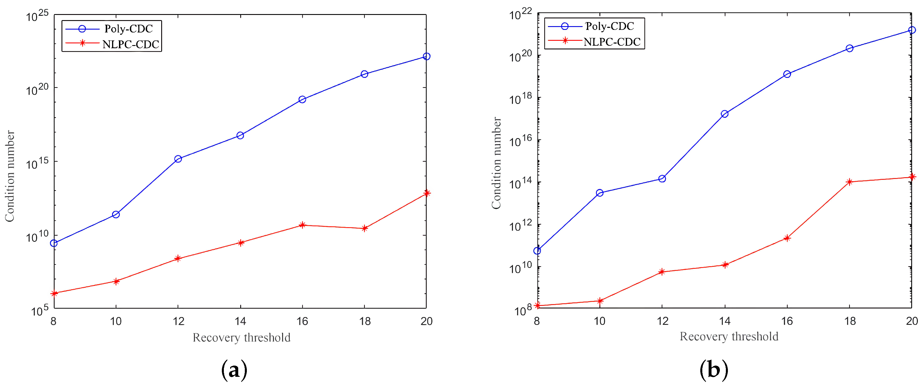
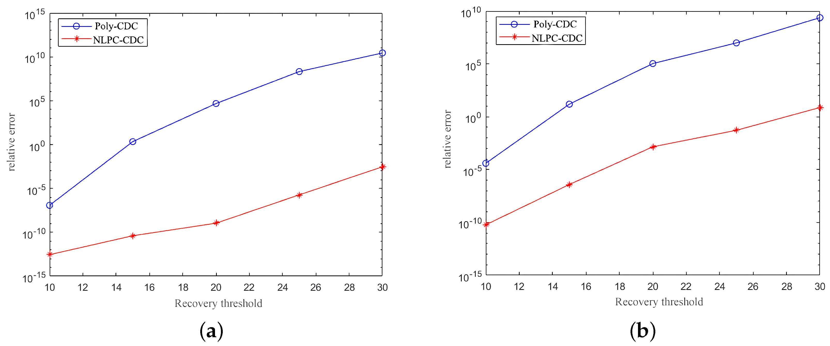
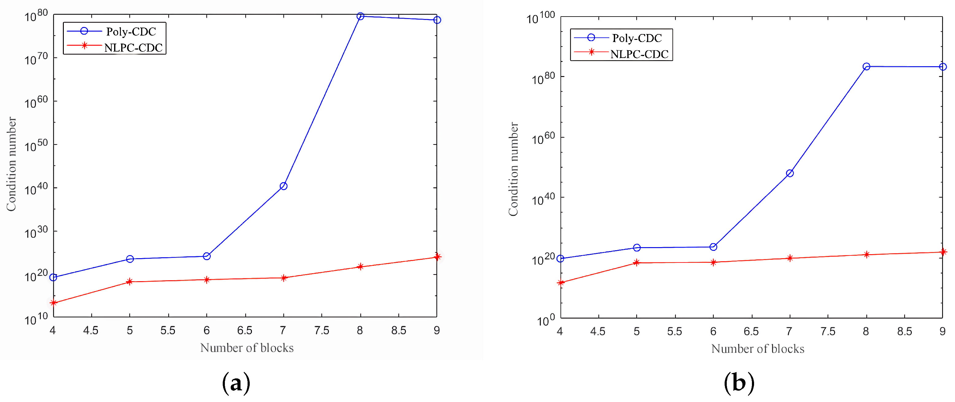
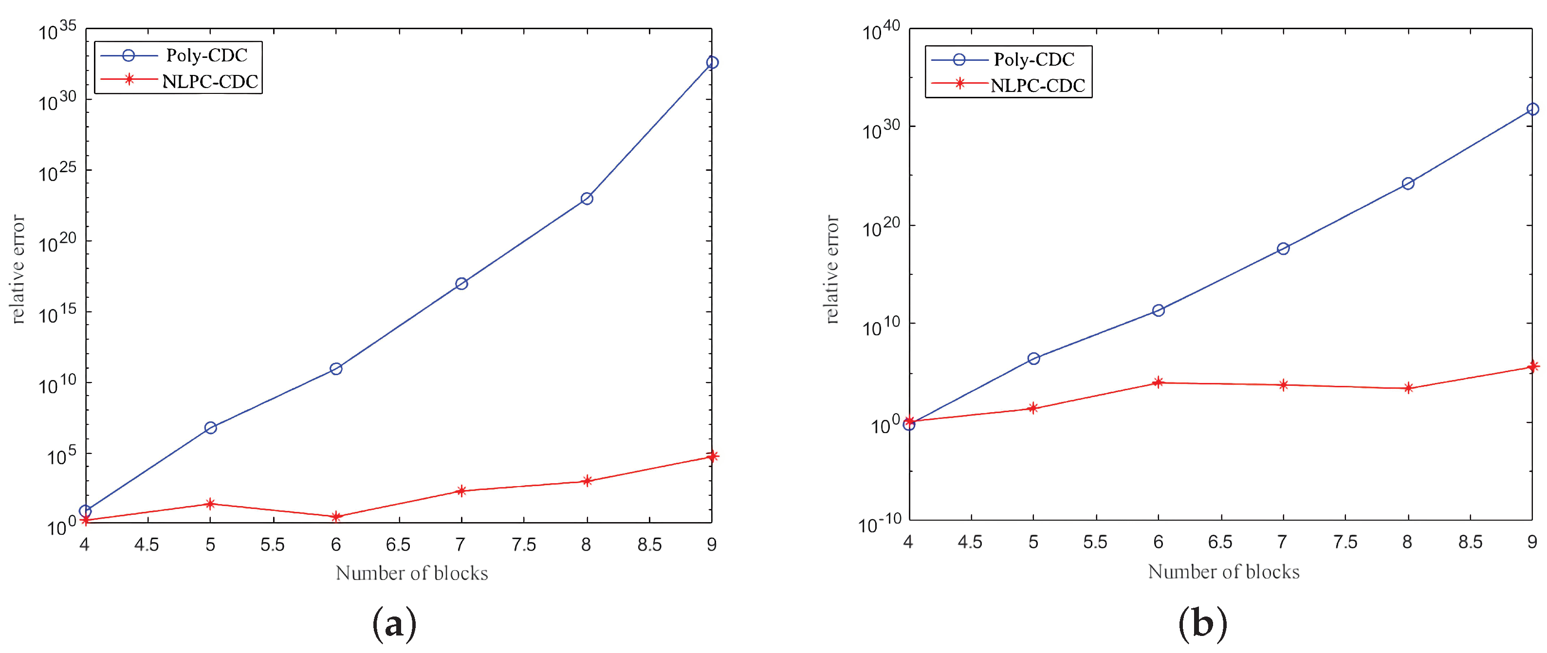
4.1. Matrix–Vector Multiplication

Condition number: The size of matrix $\mathit{A}$ and column vector $\mathit{x}$ are $5040\times 20$ and $20\times 1$, respectively. We set the number of blocks m to be from 8 to 20. We set the interpolation point to be a random number in $[0,3]$. By averaging over 50 realizations, the condition number of the Poly-CDC and NLPC-CDC versus m are plotted in Figure 3 for $N=2K$ and $N=10K$, respectively. The observations show that compared to Poly-CDC, NLPC-CDC reduces the condition number by over ${10}^{10}$ and ${10}^8$ for scenario $N=2K$ and $N=10K$, respectively.

Relative error: The size of matrix $\mathit{A}$ and column vector $\mathit{x}$ are $900\times 20$ and $20\times 1$, respectively. We set m to range from 10 to 30. The relative error of the results is plotted in Figure 4. The observations show that NLPC-CDC significantly outperforms Poly-CDC.

4.2. Matrix–Matrix Multiplication

Condition number: The size of matrix $\mathit{A}$ and $\mathit{B}$ are $2520\times 10$ and $10\times 2520$, respectively. We set the number of blocks m to be from four to nine. A random number in $[0,3]$ is selected as the interpolation point. By averaging over 50 realizations, the condition numbers of Poly-CDC and NLPC-CDC vs. m are plotted in Figure 5, for $N=2K$ and $N=10K$, respectively. The observations show that the condition number of Poly-CDC increases rapidly when the number of blocks exceeds six, while the condition number of NLPC-CDC grows very slowly for both scenarios, $N=2K$ and $N=10K$, indicating significant improvement of NLPC-CDC over Poly-CDC.

Relative error: The relatives error of the results are plotted in Figure 6. The observations show that NLPC-CDC significantly outperforms Poly-CDC.

5. Conclusions

To improve numerical stability, a novel NLPC-based CDC was proposed. A detailed design were executed for both matrix–vector and matrix–matrix multiplications. An associated proof that the constructed code possesses an $(n,k)$-symmetrical combination property (CP) was provided. A series of numerical studies verified that our proposed NLPC-CDC significantly outperforms Poly-CDC in terms of the achieved condition number or relative error, and the improvement was over ${10}^4$ for all cases. This work adopted random interpolation points, without careful selection of real interpolation points. Therefore, future work may consider selecting appropriate interpolation points to obtain the best numerical results, which variants may outperform the Poly-CDC variants [17,18]. In addition, as the encoding procedure is complicated and tedious, we may consider designing a simple encoding method that can maintain numerical stability.

References

1. Fan, M.; Hong, C.; Yingke, L. Blind Recognition of Forward Error Correction Codes Based on a Depth Distribution Algorithm. Symmetry 2021, 13, 1094. [Google Scholar] [CrossRef]
2. Abbas, N.; Zhang, Y.; Taherkordi, A. Mobile edge computing: A survey. IEEE Internet Things J. 2017, 5, 450–465. [Google Scholar] [CrossRef] [Green Version]
3. Shi, W.; Cao, J.; Zhang, Q. Edge Computing: Vision and Challenges. IEEE Internet Things J. 2016, 3, 637–646. [Google Scholar] [CrossRef]
4. Zhu, H.; Luan, T.H.; Dong, M. Guest editorial: Fog computing on wheels. Peer-Peer Netw. Appl. 2018, 11, 735–737. [Google Scholar] [CrossRef] [Green Version]
5. Wang, T.; Zhou, J.; Liu, A. Fog-Based Computing and Storage Offloading for Data Synchronization in IoT. IEEE Internet Things J. 2018, 6, 4272–4282. [Google Scholar] [CrossRef]
6. Sisinni, E.; Saifullah, A.; Han, S. Industrial internet of things: Challenges, opportunities, and directions. IEEE Internet Things J. 2018, 14, 4724–4734. [Google Scholar] [CrossRef]
7. Pokamestov, D. Adaptation of Signal with NOMA and Polar Codes to the Rayleigh Channel. Symmetry 2022, 14, 2103. [Google Scholar] [CrossRef]
8. Shen, X.; Gao, J.; Wu, W.; Li, M.; Zhou, C.; Zhuang, W. Holistic network intelligence for 6G. IEEE Commun. Surv. Tutotrials 2022, 24, 1–30. [Google Scholar] [CrossRef]
9. Li, J.; Dang, S.; Huang, Y.; Chen, P.; Qi, X.; Wen, M. Composite multiple-mode orthogonal frequency division multiplexing with index modulation. IEEE Trans. Wirel. Commun. 2022, 22, 3748–3761. [Google Scholar] [CrossRef]
10. Li, J.; Dang, S.; Wen, M.; Li, Q.; Chen, Y.; Huang, Y. Index Modulation Multiple Access for 6G Communications: Principles, Applications, and Challenges. IEEE Netw. 2023, 37, 52–60. [Google Scholar] [CrossRef]
11. Liu, N.; Li, K.; Tao, M. Code design and latency analysis of distributed matrix multiplication with straggling servers in fading channels. China Commun. 2021, 18, 15–29. [Google Scholar] [CrossRef]
12. Shin, D.-J.; Kim, J.-J. Cache-Based Matrix Technology for Efficient Write and Recovery in Erasure Coding Distributed File Systems. Symmetry 2023, 15, 872. [Google Scholar] [CrossRef]
13. Dean, J.; Barroso, L.A. The tail at scale. Commun. ACM 2013, 56, 74–80. [Google Scholar] [CrossRef]
14. Herault, T.; Hoarau, W. FAIL-MPI: How fault-tolerant is fault-tolerant MPI? In Proceedings of the IEEE International Conference on Cluster Computing, Barcelona, Spain, 25–28 September 2006. [Google Scholar]
15. Dai, M. SAZD: A low computational load coded distributed computing framework for IoT systems. IEEE Internet Things J. 2020, 7, 3640–3649. [Google Scholar] [CrossRef]
16. Yu, Q.; Maddah-Ali, M.A.; Avestimehr, A.S. Polynomial Codes: An Optimal Design for High-Dimensional Coded Matrix Multiplication. Adv. Neural Inf. Process. Syst. 2017, 30, 1–11. [Google Scholar]
17. Hasırcıoğlu, B.; Gómez-Vilardebó, J.; Gündüz, D. Bivariate Hermitian Polynomial Coding for Efficient Distributed Matrix Multiplication. In Proceedings of the IEEE Global Communications Conference, Taipei, Taiwan, 7–11 December 2020; pp. 1–6. [Google Scholar]
18. Hasırcıoğlu, B.; Gómez-Vilardebó, J.; Gündüz, D. Bivariate Polynomial Coding for Efficient Distributed Matrix Multiplication. IEEE J. Sel. Areas Inf. Theory 2021, 2, 814–829. [Google Scholar] [CrossRef]
19. Gautschi, W.; Inglese, G. Lower bounds for the condition number of vandermonde matrices. Numer. Math. 1987, 52, 241–250. [Google Scholar] [CrossRef]
20. Gautschi, W. How (un) stable are vandermonde systems. Asymptot. Comput. Anal. 1990, 124, 193–210. [Google Scholar]
21. Reichel, L.; Opfer, G. Chebyshev-vandermonde systems. Math. Comput. 1991, 57, 703–721. [Google Scholar] [CrossRef]
22. Shen, X.; Gao, J.; Wu, W. AI-assisted network-slicing based next-generation wireless networks. IEEE Open J. Veh. Technol. 2020, 1, 45–66. [Google Scholar] [CrossRef]
23. Quarteroni, A.; Sacco, R.; Saleri, F. Numerical Mathematics; Springer: Berlin/Heidelberg, Germany, 2010; Volume 37. [Google Scholar]
24. Trefethen, L.N. Approximation Theory and Approximation Practice; Society for Industrial and Applied Mathematics: Philadelphia, PA, USA, 2013; Volume 128. [Google Scholar]
Figure 1. Matrix–vector multiplication within the CDC framework.
Symmetry 15 01372 g001
Figure 2. Matrix–matrix multiplication within the CDC framework.
Symmetry 15 01372 g002
Figure 3. Condition number of matrix–vector multiplication. (a) N = 2 K . (b) N = 10 K .
Symmetry 15 01372 g003
Figure 4. Relative error of matrix–vector multiplication. (a) N = 2 K . (b) N = 10 K .
Symmetry 15 01372 g004
Figure 5. Condition number of matrix–matrix multiplication. (a) N = 2 K . (b) N = 10 K .
Symmetry 15 01372 g005
Figure 6. Relative error of matrix–matrix multiplication. (a) N = 2 K . (b) N = 10 K .
Symmetry 15 01372 g006
Disclaimer/Publisher’s Note: The statements, opinions and data contained in all publications are solely those of the individual author(s) and contributor(s) and not of MDPI and/or the editor(s). MDPI and/or the editor(s) disclaim responsibility for any injury to people or property resulting from any ideas, methods, instructions or products referred to in the content.