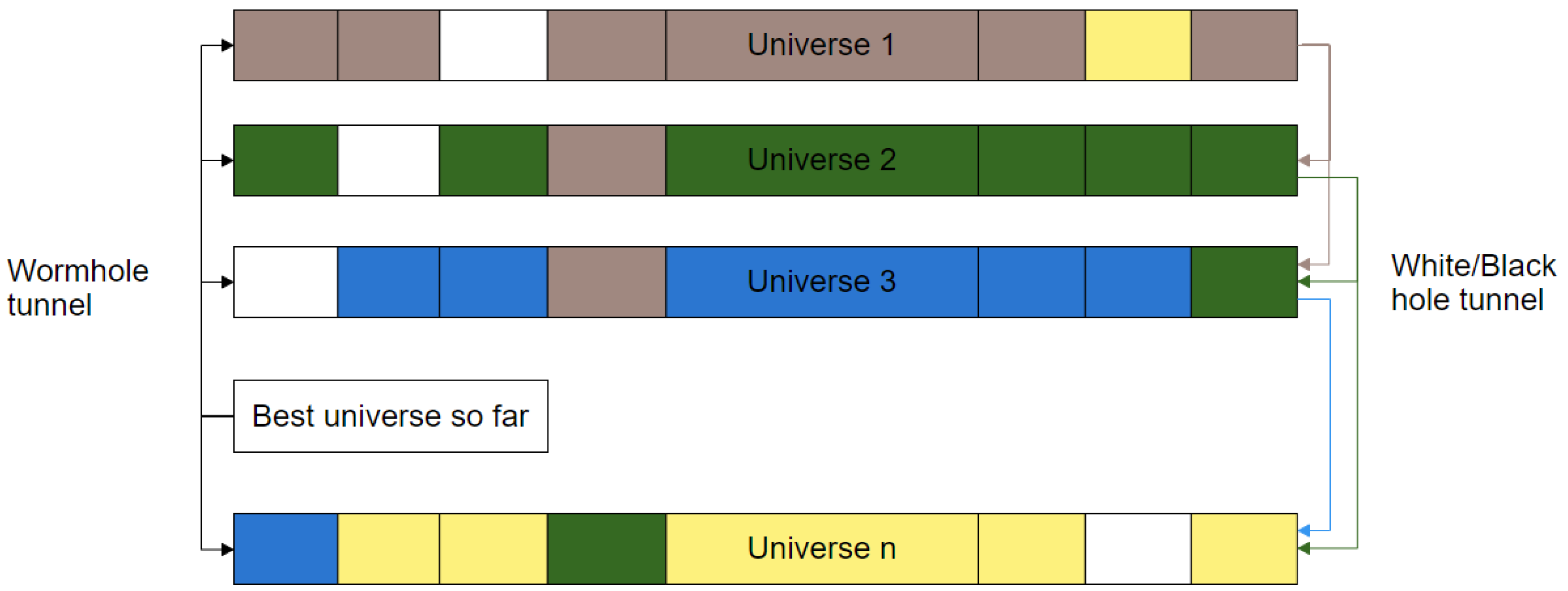
Figure 1.
Concepts of cosmology implemented in MVO algorithm.
Figure 1.
Concepts of cosmology implemented in MVO algorithm.
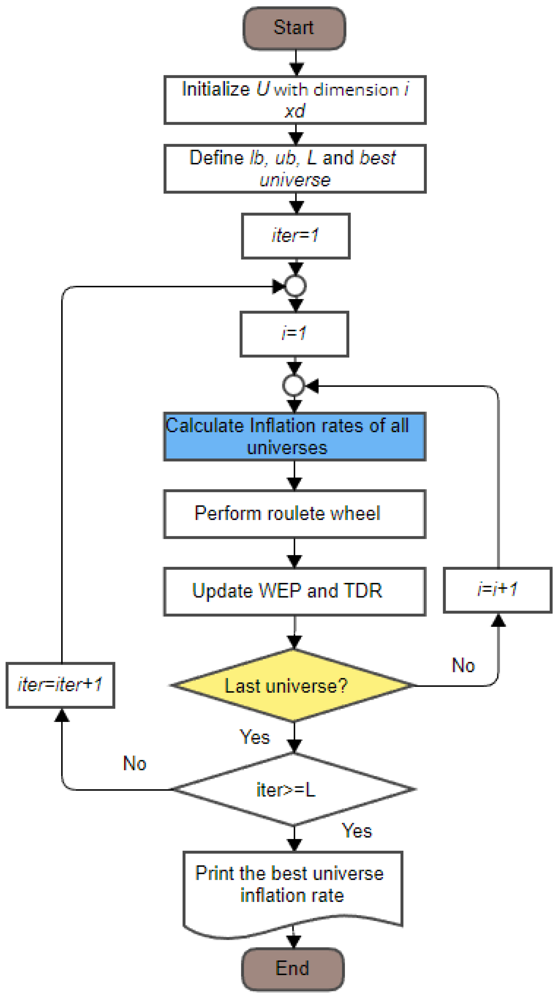
Figure 2.
MVO algorithm flowchart representation.
Figure 2.
MVO algorithm flowchart representation.
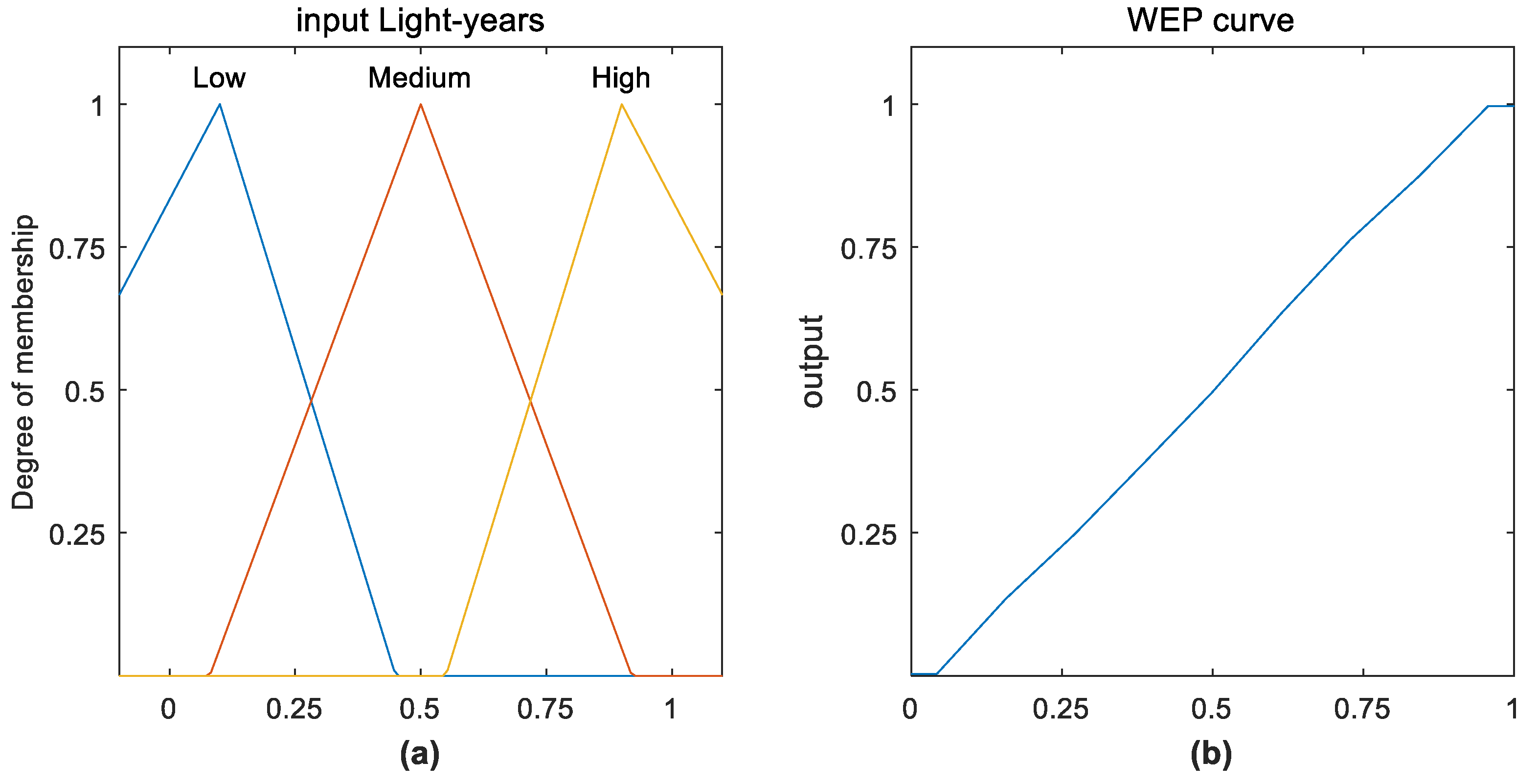
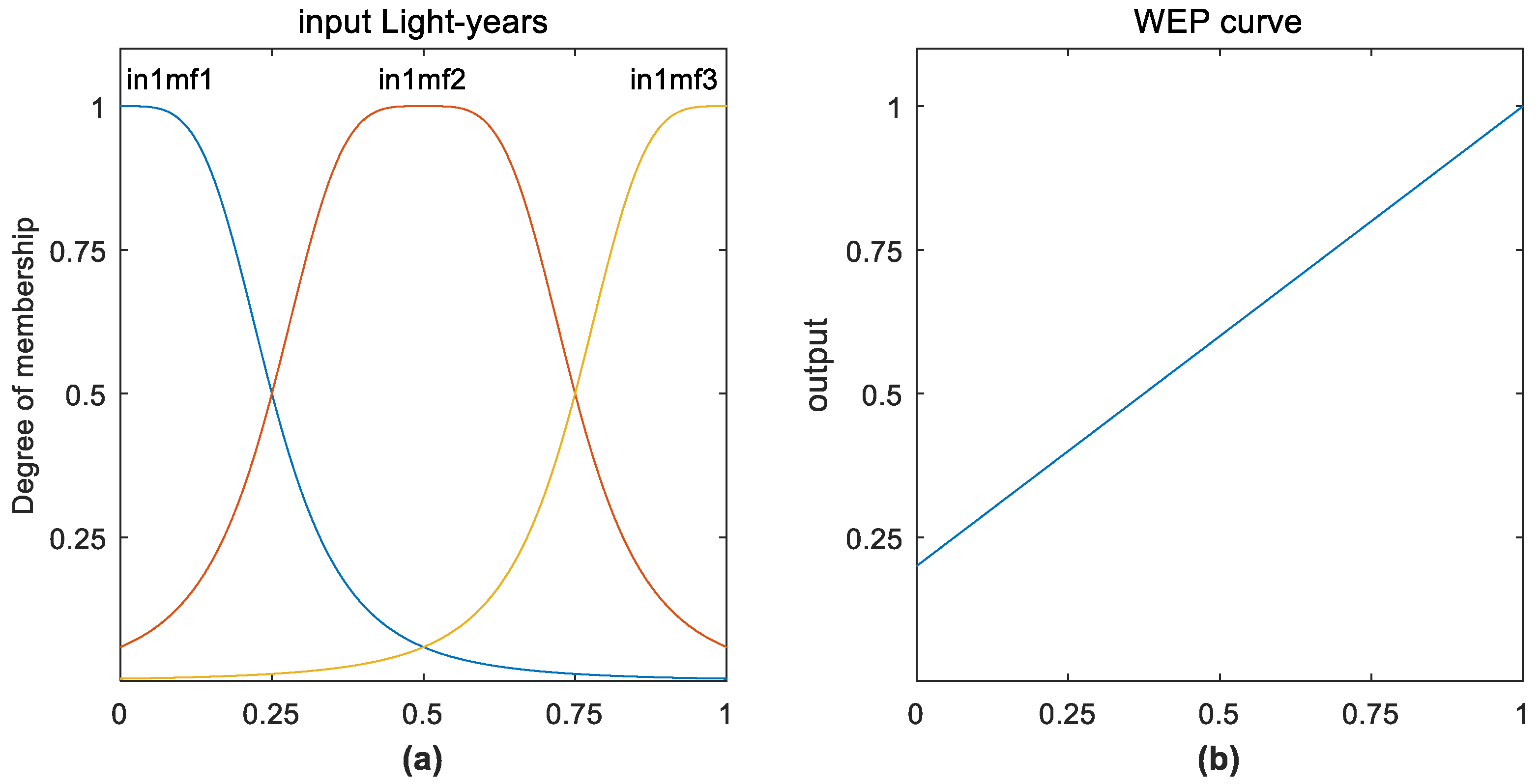
Figure 3.
Mamdani model for WEP. (a) Input light-years of fuzzy inference system; (b) output obtained for WEP of fuzzy inference system using centroid defuzzification method.
Figure 3.
Mamdani model for WEP. (a) Input light-years of fuzzy inference system; (b) output obtained for WEP of fuzzy inference system using centroid defuzzification method.
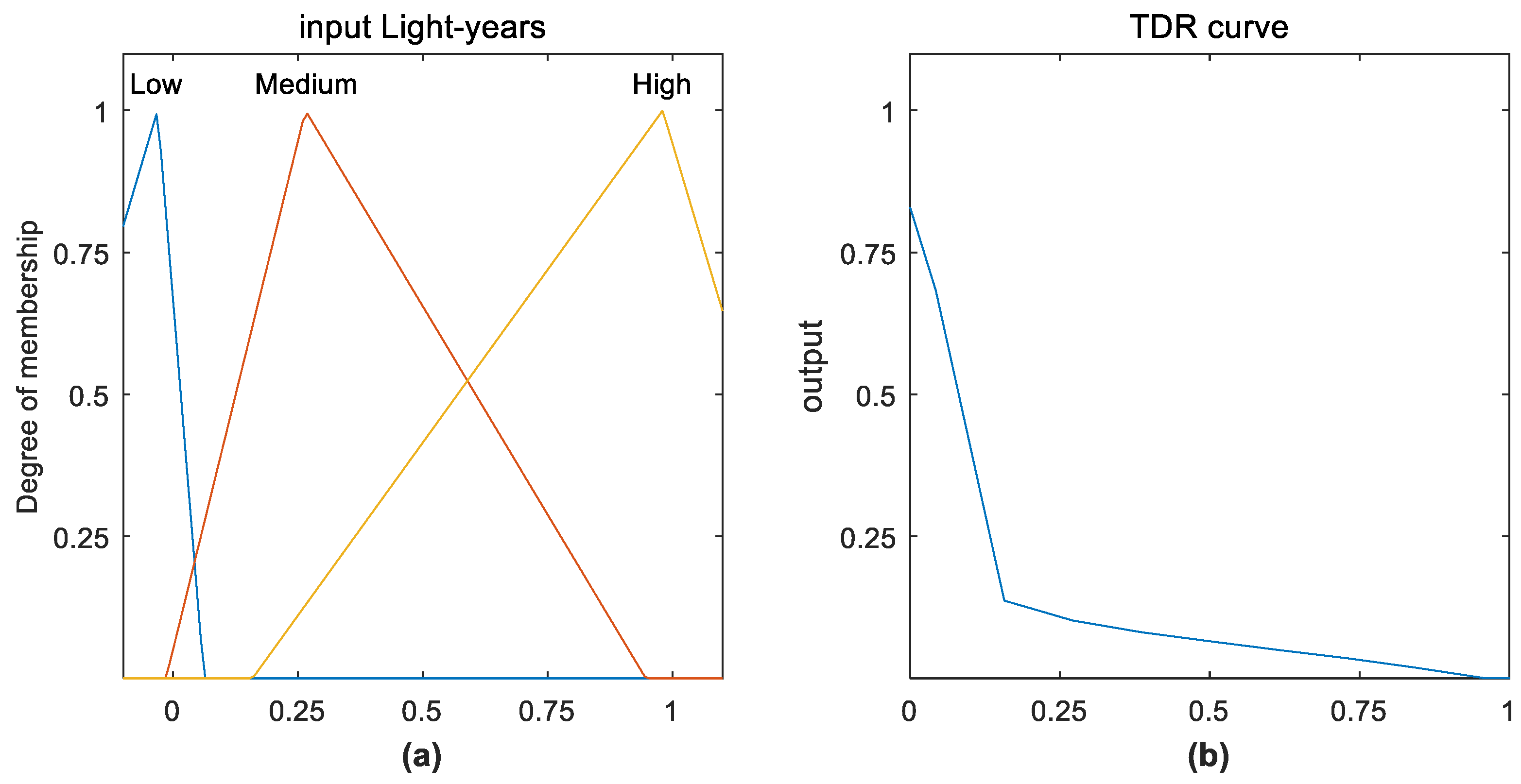
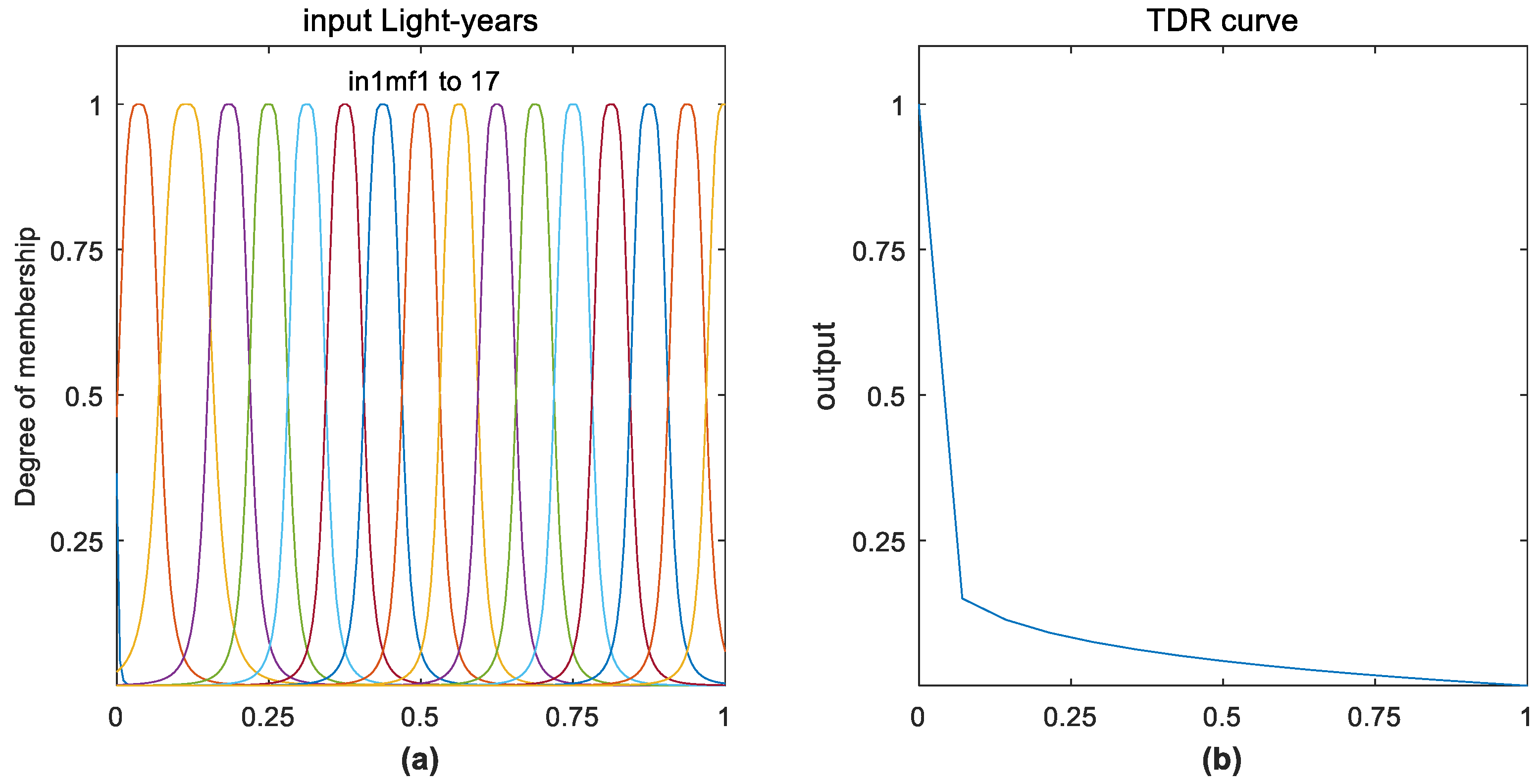
Figure 4.
Mamdani model for TDR. (a) Input light-years of fuzzy inference system; (b) output obtained for TDR of fuzzy inference system using centroid defuzzification method.
Figure 4.
Mamdani model for TDR. (a) Input light-years of fuzzy inference system; (b) output obtained for TDR of fuzzy inference system using centroid defuzzification method.
Figure 5.
Sugeno model for WEP. (a) Input light-years of fuzzy inference system; (b) output obtained for WEP of fuzzy inference system using weighted average defuzzification method.
Figure 5.
Sugeno model for WEP. (a) Input light-years of fuzzy inference system; (b) output obtained for WEP of fuzzy inference system using weighted average defuzzification method.
Figure 6.
Sugeno model for TDR. (a) Input light-years of fuzzy inference system; (b) output obtained for TDR of fuzzy inference system using weighted average defuzzification method.
Figure 6.
Sugeno model for TDR. (a) Input light-years of fuzzy inference system; (b) output obtained for TDR of fuzzy inference system using weighted average defuzzification method.
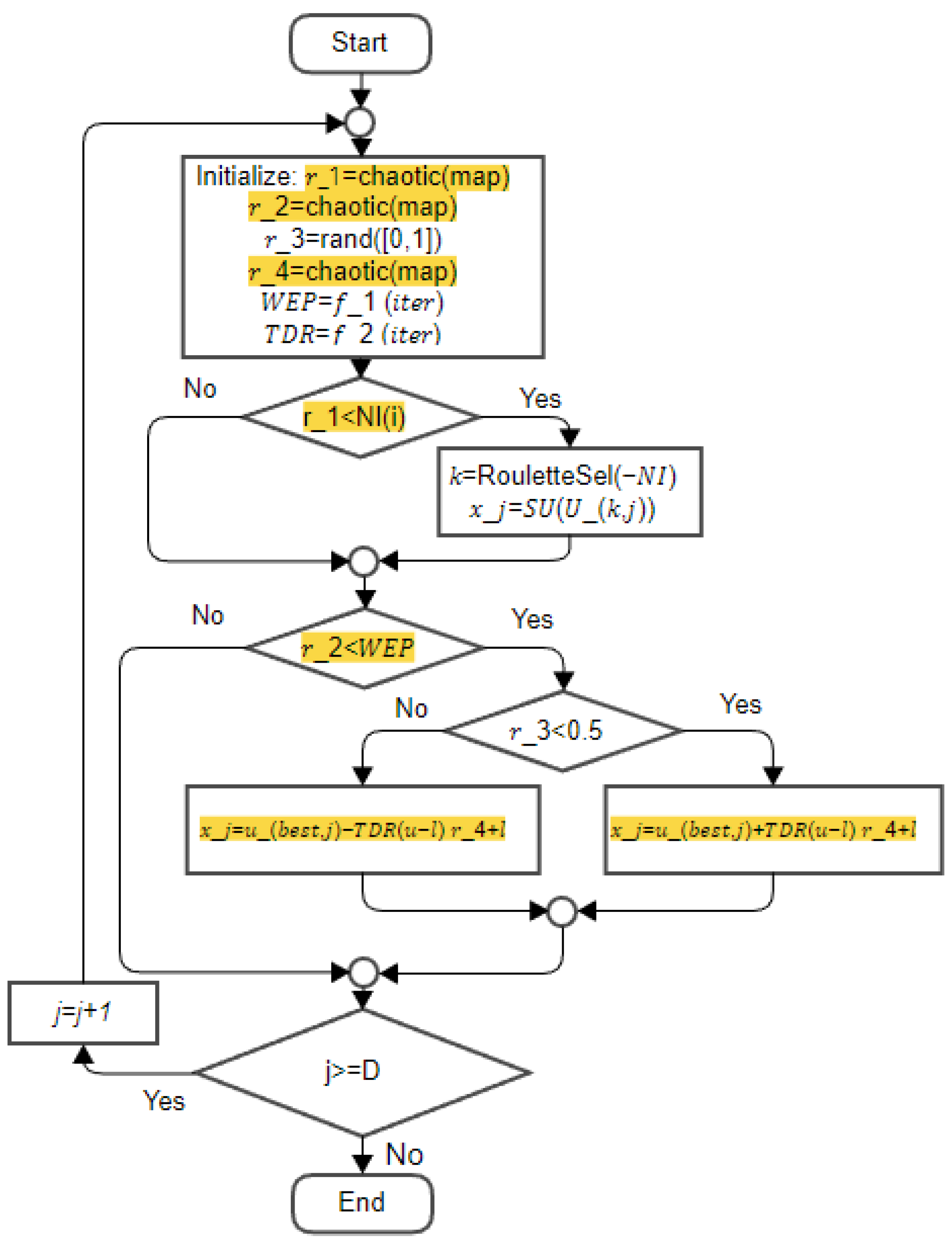
Figure 7.
MVO flowchart for the process of selection of universes with chaotic maps adaptation.
Figure 7.
MVO flowchart for the process of selection of universes with chaotic maps adaptation.
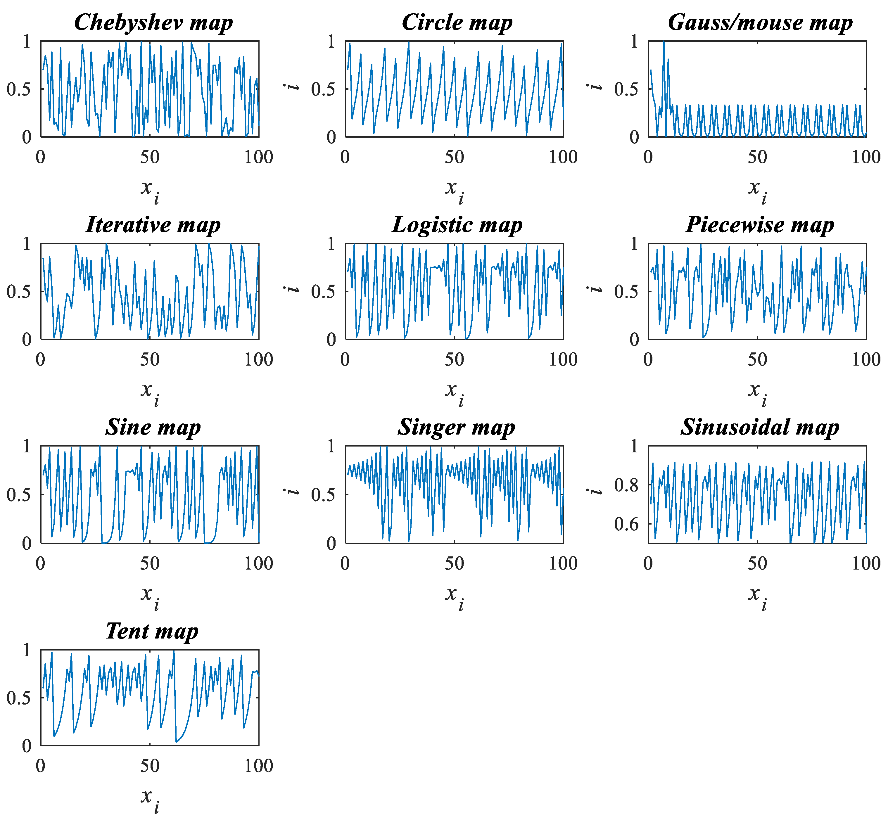
Figure 8.
Representation of chaotic maps in
Table 1 with 100 iterations.
Figure 8.
Representation of chaotic maps in
Table 1 with 100 iterations.
Figure 9.
Bifurcation map of chaotic maps in
Table 6.
Figure 9.
Bifurcation map of chaotic maps in
Table 6.
Table 1.
Membership function parameters for WEP Mamdani fuzzy inference system.
Table 1.
Membership function parameters for WEP Mamdani fuzzy inference system.
| Linguistic Variable | Linguistic Value | a | b | c |
|---|
| Light-years | Low | −0.5 | 0.1 | 0.45 |
| Medium | 0.08 | 0.5 | 0.92 |
| High | 0.55 | 0.9 | 1.5 |
| WEP | Low | −0.15 | 0 | 0.16 |
| Medium | 0.33 | 0.5 | 0.66 |
| High | 0.82 | 1 | 1.17 |
Table 2.
Membership function parameters for TDR Mamdani fuzzy inference system.
Table 2.
Membership function parameters for TDR Mamdani fuzzy inference system.
| Linguistic Variable | Linguistic Value | a | b | c |
|---|
| Light-years | Low | −0.369 | −0.0312 | 0.0619 |
| Medium | −0.0143 | 0.265 | 0.9466 |
| High | 0.159 | 0.9804 | 1.32 |
| TDR | Low | −0.2268 | 0.002633 | 0.2262 |
| Medium | −0.03122 | 0.0915 | 0.337 |
| High | 0.832 | 1.052 | 1.34 |
Table 3.
Membership function parameters for WEP Sugeno fuzzy inference system.
Table 3.
Membership function parameters for WEP Sugeno fuzzy inference system.
| Linguistic Variable | Linguistic Value | a | b | c |
|---|
| Light-years | in1mf1 | 0.25 | 2 | 0 |
| in1mf2 | 0.25 | 2 | 0.5 |
| in1mf3 | 0.25 | 2 | 1 |
Table 4.
Membership function parameters for the TDR Sugeno fuzzy inference system.
Table 4.
Membership function parameters for the TDR Sugeno fuzzy inference system.
| Linguistic Variable | Linguistic Value | a | b | c |
|---|
| Light-years | in1mf1 | 0.005371 | 2.001 | −0.006169 |
| in1mf2 | 0.03512 | 2 | 0.03649 |
| in1mf3 | 0.04512 | 2 | 0.1143 |
| in1mf4 | 0.0352 | 2 | 0.1845 |
| in1mf5 | 0.03214 | 2 | 0.2493 |
| in1mf6 | 0.03147 | 2 | 0.3124 |
| in1mf7 | 0.03131 | 2 | 0.375 |
| in1mf8 | 0.03127 | 2 | 0.4375 |
| in1mf9 | 0.03126 | 2 | 0.5 |
| in1mf10 | 0.03125 | 2 | 0.5625 |
| in1mf11 | 0.03125 | 2 | 0.625 |
| in1mf12 | 0.03125 | 2 | 0.6875 |
| in1mf13 | 0.03125 | 2 | 0.75 |
| in1mf14 | 0.03125 | 2 | 0.8125 |
| in1mf15 | 0.03125 | 2 | 0.875 |
| in1mf16 | 0.03125 | 2 | 0.9375 |
| in1mf17 | 0.03125 | 2 | 1 |
Table 5.
Fuzzy rules set for the fuzzy inference systems.
Table 5.
Fuzzy rules set for the fuzzy inference systems.
| System | Fuzzy Rules |
|---|
| Mamdani WEP | 1. If Light-years is Low, then WEP is Low |
| 2. If Light-years is Medium, then WEP is Medium |
| 3. If Light-years is High, then WEP is High |
| Mamdani TDR | 1. If Lightyears is Low, then TDR is High |
| 2. If Lightyears is Medium then, TDR is Medium |
| 3. If Lightyears is High then, TDR is Low |
| Sugeno WEP | 1. If input1 is in1mf1, then output is out1mf1 |
| 2. If input1 is in1mf2, then output is out1mf2 |
| 3. If input1 is in1mf3, then output is out1mf3 |
| Sugeno TDR | 1. If input1 is in1mf1, then output is out1mf1 |
| 2. If input1 is in1mf2, then output is out1mf2 |
| 3. If input1 is in1mf3, then output is out1mf3 |
| 4. If input1 is in1mf4, then output is out1mf4 |
| 5. If input1 is in1mf5, then output is out1mf5 |
| 6. If input1 is in1mf6, then output is out1mf6 |
| 7. If input1 is in1mf7, then output is out1mf7 |
| 8. If input1 is in1mf8, then output is out1mf8 |
| 9. If input1 is in1mf9, then output is out1mf9 |
| 10. If input1 is in1mf10, then output is out1mf10 |
| 11. If input1 is in1mf11, then output is out1mf11 |
| 12. If input1 is in1mf12, then output is out1mf12 |
| 13. If input1 is in1mf13, then output is out1mf13 |
| 14. If input1 is in1mf14, then output is out1mf14 |
| 15. If input1 is in1mf15, then output is out1mf15 |
| 16. If input1 is in1mf16, then output is out1mf16 |
| 17. If input1 is in1mf17, then output is out1mf17 |
Table 6.
Chaotic maps of the literature [
19], using seed
p = 0.7.
Table 6.
Chaotic maps of the literature [
19], using seed
p = 0.7.
| Name | Equation | Parameters |
|---|
| Chebyshev [31] | | |
| Logistic [32] | | |
| Sinusoidal [33] | | |
| Circle [34] | |
|
| Gauss/mouse [35] | | |
| Iterative [32] | | |
| Piecewise [36] | | |
| Sine [37] | | |
| Singer [38] | | |
| Tent [39] | | |
Table 7.
Chaotic variants of MVO algorithm.
Table 7.
Chaotic variants of MVO algorithm.
| Variant Name | | | |
|---|
| R1 | Chaotic map [0,1] | Random [0,1] | Random [0,1] |
| R2 | Random [0,1] | Chaotic map [0,1] | Random [0,1] |
| R4 | Random [0,1] | Random [0,1] | Chaotic map [0,1] |
| RT | Chaotic map [0,1] | Chaotic map [0,1] | Chaotic map [0,1] |
Table 8.
Results comparing MVO with R1 CMVO in 50 dimensions.
Table 8.
Results comparing MVO with R1 CMVO in 50 dimensions.
| Variant | MVO | CMVO Circle | CMVO Sinusoidal | CMVO Gauss |
|---|
| Function | Average | SD | Average | SD | Z | Average | SD | Z | Average | SD | Z |
|---|
| F1 | 1.04 × 101 | 2.12 × 100 | 6.05 × 100 | 1.32 × 100 | −9.55 | 6.18 × 100 | 1.16 × 100 | −9.57 | 8.80 × 100 | 2.23 × 100 | −2.85 |
| F2 | 4.29 × 10² | 1.40 × 10³ | 1.43 × 10² | 9.27 × 101 | −1.11 | 8.24 × 101 | 7.40 × 101 | −1.35 | 3.41 × 100 | 1.20 × 100 | −1.66 |
| F3 | 5.87 × 10³ | 1.42 × 10³ | 6.62 × 10² | 2.02 × 10³ | 1.68 | 6.50 × 10³ | 1.70 × 10³ | 1.57 | 5.01 × 10³ | 1.66 × 10³ | −2.15 |
| F4 | 1.66 × 101 | 6.53 × 100 | 3.14 × 101 | 7.54 × 100 | 8.13 | 2.14 × 101 | 5.14 × 100 | 3.12 | 9.23 × 100 | 2.06 × 100 | −5.93 |
| F5 | 6.64 × 10² | 6.96 × 10² | 1.14 × 10³ | 9.97 × 10² | 2.14 | 1.08 × 10³ | 8.07 × 10² | 2.12 | 1.01 × 10³ | 1.05 × 10³ | 1.49 |
| F6 | 1.06 × 101 | 2.71 × 100 | 5.86 × 100 | 1.57 × 100 | −8.23 | 6.39 × 100 | 1.37 × 100 | −7.54 | 9.76 × 100 | 3.06 × 100 | −1.09 |
| F7 | 1.19 × 10⁻¹ | 4.03 × 10⁻² | 1.08 × 10⁻¹ | 3.39 × 10⁻² | −1.20 | 1.12 × 10⁻¹ | 3.64 × 10⁻² | −0.67 | 9.64 × 10⁻² | 2.91 × 10⁻² | −2.51 |
| F8 | 1.25 × 10⁴ | 8.00 × 10² | 1.22 × 10⁴ | 8.37 × 10² | −1.37 | 1.22 × 10⁴ | 9.58 × 10² | −1.11
| 1.28 × 10⁴ | 1.01 × 10³ | 1.43 |
| F9 | 2.54 × 10² | 4.94 × 101 | 2.34 × 10² | 4.61 × 101 | −1.58 | 2.04 × 10² | 3.70 × 101 | −4.42 | 2.33 × 10² | 4.87 × 101 | −1.68 |
| F10 | 3.49 × 100 | 3.08 × 100 | 3.04 × 100 | 4.60 × 10⁻¹ | −0.80 | 2.43 × 100 | 4.22 × 10⁻¹ | −1.86 | 3.15 × 100 | 5.99 × 10⁻¹ | −0.59 |
| F11 | 1.09 × 100 | 1.82 × 10⁻² | 1.05 × 100 | 1.38 × 10⁻² | −8.70 | 1.05 × 100 | 1.39 × 10⁻² | −9.12 | 1.09 × 100 | 2.07 × 10⁻² | −0.05 |
| F12 | 6.57 × 100 | 2.64 × 100 | 7.90 × 100 | 2.78 × 100 | 1.89 | 4.91 × 100 | 2.50 × 100 | −2.49 | 4.93 × 100 | 2.34 × 100 | −2.54 |
| F13 | 9.08 × 100 | 1.34 × 101 | 6.56 × 100 | 7.21 × 100 | −0.91 | 4.61 × 100 | 6.30 × 100 | −1.66 | 2.90 × 100 | 2.61 × 100 | −2.48 |
Table 9.
Results comparing MVO with R2 CMVO in 50 dimensions.
Table 9.
Results comparing MVO with R2 CMVO in 50 dimensions.
| Variant | MVO | CMVO Iterative | CMVO Sinusoidal | CMVO Gauss |
|---|
| Function | Average | SD | Average | SD | Z | Average | SD | Z | Average | SD | Z |
|---|
| F1 | 1.04 × 101 | 2.12 × 100 | 9.44 × 100 | 2.31 × 100 | −1.67 | 1.03 × 101 | 2.00 × 100 | −0.28 | 1.13 × 101 | 2.85 × 100 | 1.42 |
| F2 | 4.29 × 10² | 1.40 × 10³ | 2.16 × 10⁴ | 1.18 × 10⁵ | 0.99 | 1.87 × 10⁷ | 7.84 × 10⁷ | 1.31 | 5.52 × 10¹⁰ | 3.01 × 10¹¹ | 1 |
| F3 | 5.87 × 10³ | 1.42 × 10³ | 6.98 × 10³ | 1.85 × 10³ | 2.62 | 8.23 × 10³ | 1.76 × 10³ | 5.72 | 5.94 × 10³ | 1.39 × 10³ | 0.21 |
| F4 | 1.66 × 101 | 6.53 × 100 | 1.99 × 101 | 6.39 × 100 | 1.96 | 3.24 × 101 | 6.94 × 100 | 9.04 | 1.67 × 101 | 5.15 × 100 | 0.02 |
| F5 | 6.64 × 10² | 6.96 × 10² | 1.32 × 10³ | 1.18 × 10³ | 2.64 | 9.31 × 10² | 1.32 × 10³ | 0.98 | 1.13 × 10³ | 1.72 × 10³ | 1.37 |
| F6 | 1.06 × 101 | 2.71 × 100 | 1.04 × 101 | 1.89 × 100 | −0.3 | 1.01 × 101 | 2.34 × 100 | −0.68 | 9.66 × 100 | 2.33 × 100 | −1.4 |
| F7 | 1.19 × 10⁻¹ | 4.03 × 10⁻² | 1.09 × 10⁻¹ | 2.96 × 10⁻² | −1.16 | 1.24 × 10⁻¹ | 4.16 × 10⁻² | 0.44 | 1.17 × 10⁻¹ | 2.82 × 10⁻² | −0.25 |
| F8 | 1.25 × 10⁴ | 8.00 × 10² | 1.21 × 10⁴ | 8.04 × 10² | −1.86 | 1.27 × 10⁴ | 1.08 × 10³ | 1.13 | 1.24 × 10⁴ | 6.57 × 10² | −0.32 |
| F9 | 2.54 × 10² | 4.94 × 101 | 2.62 × 10² | 3.96 × 101 | 0.67 | 2.16 × 10² | 3.26 × 101 | −3.47 | 2.74 × 10² | 4.99 × 101 | 1.59 |
| F10 | 3.49 × 100 | 3.08 × 100 | 3.54 × 100 | 3.01 × 100 | 0.06 | 7.02 × 100 | 6.82 × 100 | 2.58 | 3.50 × 100 | 3.17 × 100 | 0.02 |
| F11 | 1.09 × 100 | 1.82 × 10⁻² | 1.10 × 100 | 2.05 × 10⁻² | 1.24 | 1.09 × 100 | 1.79 × 10⁻² | 0.11 | 1.09 × 100 | 1.63 × 10⁻² | 0.03 |
| F12 | 6.57 × 100 | 2.64 × 100 | 7.45 × 100 | 3.16 × 100 | 1.16 | 8.47 × 100 | 2.33 × 100 | 2.95 | 5.99 × 100 | 1.67 × 100 | −1.02 |
| F13 | 9.08 × 100 | 1.34 × 101 | 1.58 × 101 | 1.68 × 101 | 1.72 | 1.19 × 101 | 1.23 × 101 | 0.84 | 8.22 × 100 | 1.09 × 101 | −0.27 |
Table 10.
Results comparing MVO with R4 CMVO in 50 dimensions.
Table 10.
Results comparing MVO with R4 CMVO in 50 dimensions.
| Variant | MVO | CMVO Circle | CMVO Sinusoidal | CMVO Piecewise |
|---|
| Function | Average | SD | Average | SD | Z | Average | SD | Z | Average | SD | Z |
|---|
| F1 | 1.04 × 101 | 2.12 × 100 | 6.05 × 100 | 1.32 × 100 | −9.55 | 8.43 × 100 | 2.33 × 100 | −3.44 | 6.18 × 100 | 1.16 × 100 | −9.57 |
| F2 | 4.29 × 10² | 1.40 × 10³ | 1.43 × 10² | 9.27 × 101 | −1.11 | 2.08 × 10² | 4.29 × 10² | −0.83 | 8.24 × 101 | 7.40 × 101 | −1.35 |
| F3 | 5.87 × 10³ | 1.42 × 10³ | 6.62 × 10³ | 2.02 × 10³ | 1.68 | 6.84 × 10³ | 2.01 × 10³ | 2.17 | 6.50 × 10³ | 1.70 × 10³ | 1.57 |
| F4 | 1.66 × 101 | 6.53 × 100 | 3.14 × 101 | 7.54 × 100 | 8.13 | 3.16 × 101 | 7.33 × 100 | 8.36 | 2.14 × 101 | 5.14 × 100 | 3.12 |
| F5 | 6.64 × 10² | 6.96 × 10² | 1.14 × 10³ | 9.97 × 10² | 2.14 | 8.82 × 10² | 6.63 × 10² | 1.24 | 1.08 × 10³ | 8.07 × 10² | 2.12 |
| F6 | 1.06 × 101 | 2.71 × 100 | 5.86 × 100 | 1.57 × 100 | −8.23 | 8.62 × 100 | 1.71 × 100 | −3.35 | 6.39 × 100 | 1.37 × 100 | −7.54 |
| F7 | 1.19 × 10⁻¹ | 4.03 × 10⁻² | 1.08 × 10⁻¹ | 3.39 × 10⁻² | −1.2 | 1.19 × 10⁻¹ | 3.35 × 10⁻² | −0.05 | 1.12 × 10⁻¹ | 3.64 × 10⁻² | −0.67 |
| F8 | 1.25 × 10⁴ | 8.00 × 10² | 1.22 × 10⁴ | 8.37 × 10² | −1.37 | 1.19 × 10⁴ | 8.61 × 10² | −2.68 | 1.22 × 10⁴ | 9.58 × 10² | −1.11 |
| F9 | 2.54 × 10² | 4.94 × 101 | 2.34 × 10² | 4.61 × 101 | −1.58 | 2.51 × 10² | 4.43 × 101 | −0.26 | 2.04 × 10² | 3.70 × 101 | −4.42 |
| F10 | 3.49 × 100 | 3.08 × 100 | 3.04 × 100 | 4.60 × 10⁻¹ | −0.8 | 3.86 × 100 | 3.04 × 100 | 0.47 | 2.43 × 100 | 4.22 × 10⁻¹ | −1.86 |
| F11 | 1.09 × 100 | 1.82 × 10⁻² | 1.05 × 100 | 1.38 × 10⁻² | −8.7 | 1.08 × 100 | 1.35 × 10⁻² | −2.58 | 1.05 × 100 | 1.39 × 10⁻² | −9.12 |
| F12 | 6.57 × 100 | 2.64 × 100 | 7.90 × 100 | 2.78 × 100 | 1.89 | 8.71 × 100 | 3.25 × 100 | 2.8 | 4.91 × 100 | 2.50 × 100 | −2.49 |
| F13 | 9.08 × 100 | 1.34 × 101 | 6.56 × 100 | 7.21 × 100 | −0.91 | 1.13 × 101 | 1.09 × 101 | 0.69 | 4.61 × 100 | 6.30 × 100 | −1.66 |
Table 11.
Results comparing MVO with RT CMVO in 50 dimensions.
Table 11.
Results comparing MVO with RT CMVO in 50 dimensions.
| Variant | MVO | CMVO Circle | CMVO Gauss | CMVO Tent |
|---|
| Function | Average | SD | Average | SD | Z | Average | SD | Z | Average | SD | Z |
|---|
| F1 | 1.04 × 101 | 2.12 × 100 | 8.31 × 100 | 2.01 × 100 | −3.92 | 6.47 × 100 | 1.72 × 100 | −7.9 | 9.44 × 100 | 1.71 × 100 | −1.93 |
| F2 | 4.29 × 10² | 1.40 × 10³ | 6.61 × 10¹¹ | 3.62 × 10¹² | 1 | 1.23 × 10¹¹ | 6.32 × 10¹¹ | 1.07 | 2.11 × 10¹² | 8.93 × 10¹² | 1.29 |
| F3 | 5.87 × 10³ | 1.42 × 10³ | 1.05 × 10⁴ | 1.98 × 10³ | 10.35 | 8.46 × 10³ | 2.12 × 10³ | 5.57 | 1.17 × 10⁴ | 2.18 × 10³ | 12.31 |
| F4 | 1.66 × 101 | 6.53 × 100 | 5.54 × 101 | 8.87 × 100 | 19.29 | 6.47 × 101 | 7.69 × 100 | 26.08 | 6.14 × 101 | 6.85 × 100 | 25.9 |
| F5 | 6.64 × 10² | 6.96 × 10² | 3.31 × 10³ | 5.28 × 10³ | 2.72 | 1.04 × 10³ | 1.17 × 10³ | 1.5 | 2.60 × 10³ | 4.29 × 10³ | 2.44 |
| F6 | 1.06 × 101 | 2.71 × 100 | 8.57 × 100 | 2.18 × 100 | −3.16 | 6.93 × 100 | 1.31 × 100 | −6.63 | 9.37 × 100 | 1.64 × 100 | −2.08 |
| F7 | 1.19 × 10⁻¹ | 4.03 × 10⁻² | 2.09 × 10⁻¹ | 5.78 × 10⁻² | 6.99 | 1.71 × 10⁻¹ | 6.97 × 10⁻² | 3.53 | 2.22 × 10⁻¹ | 6.97 × 10⁻² | 7 |
| F8 | 1.25 × 10⁴ | 8.00 × 10² | 1.17 × 10⁴ | 7.49 × 10² | −3.59 | 1.17 × 10⁴ | 8.21 × 10² | −3.63 | 1.19 × 10⁴ | 9.46 × 10² | −2.42 |
| F9 | 2.54 × 10² | 4.94 × 101 | 1.89 × 10² | 3.19 × 101 | −6.05 | 1.73 × 10² | 2.17 × 101 | −8.21 | 2.23 × 10² | 2.92 × 101 | −2.96 |
| F10 | 3.49 × 100 | 3.08 × 100 | 4.88 × 100 | 4.78 × 10⁻¹ | 2.44 | 4.67 × 100 | 5.58 × 10⁻¹ | 2.05 | 5.68 × 100 | 2.65 × 100 | 2.95 |
| F11 | 1.09 × 100 | 1.82 × 10⁻² | 1.08 × 100 | 1.61 × 10⁻² | −2.3 | 1.06 × 100 | 1.82 × 10⁻² | −6.42 | 1.08 × 100 | 1.46 × 10⁻² | −1.94 |
| F12 | 6.57 × 100 | 2.64 × 100 | 1.89 × 101 | 6.33 × 100 | 9.81 | 2.48 × 101 | 1.15 × 101 | 8.47 | 2.56 × 101 | 9.02 × 100 | 11.11 |
| F13 | 9.08 × 100 | 1.34 × 101 | 7.07 × 101 | 3.39 × 101 | 9.26 | 7.30 × 101 | 3.52 × 101 | 9.3 | 8.32 × 101 | 3.73 × 101 | 10.25 |
Table 12.
Results comparing MVO with R1 FCMVO Mamdani using a Circle map in 50 dimensions.
Table 12.
Results comparing MVO with R1 FCMVO Mamdani using a Circle map in 50 dimensions.
| Variant | FCMVO Mamdani | MVO | MVO Circle | FMVO Mamdani |
|---|
| Function | Average | SD | Average | SD | Z | Average | SD | Z | Average | SD | Z |
|---|
| F1 | 4.18 × 100 | 1.50 × 100 | 1.04 × 101 | 2.12 × 100 | −13.12 | 1.06 × 101 | 2.37 × 100 | −12.46 | 4.22 × 100 | 1.54 × 100 | −0.1 |
| F2 | 2.13 × 10³ | 1.09 × 10⁴ | 4.29 × 10² | 1.40 × 10³ | 0.85 | 4.65 × 10² | 1.28 × 10³ | 0.83 | 1.84 × 10² | 3.50 × 10² | 0.98 |
| F3 | 4.69 × 10³ | 1.27 × 10³ | 5.87 × 10³ | 1.42 × 10³ | −3.38 | 6.29 × 10³ | 1.89 × 10³ | −3.85 | 4.46 × 10³ | 1.32 × 10³ | 0.68 |
| F4 | 2.43 × 101 | 6.58 × 100 | 1.66 × 101 | 6.53 × 100 | 4.52 | 1.86 × 101 | 5.21 × 100 | 3.71 | 1.69 × 101 | 7.05 × 100 | 4.21 |
| F5 | 6.58 × 10² | 7.15 × 10² | 6.64 × 10² | 6.96 × 10² | −0.03 | 6.41 × 10² | 5.19 × 10² | 0.11 | 5.02 × 10² | 5.32 × 10² | 0.96 |
| F6 | 3.94 × 100 | 1.65 × 100 | 1.06 × 101 | 2.71 × 100 | −11.45 | 1.03 × 101 | 2.52 × 100 | −11.5 | 4.05 × 100 | 1.38 × 100 | −0.3 |
| F7 | 8.77 × 10⁻² | 2.57 × 10⁻² | 1.19 × 10⁻¹ | 4.03 × 10⁻² | −3.61 | 1.24 × 10⁻¹ | 4.27 × 10⁻² | −4.05 | 7.71 × 10⁻² | 2.46 × 10⁻² | 1.62 |
| F8 | 1.19 × 10⁴ | 9.07 × 10² | 1.25 × 10⁴ | 8.00 × 10² | −2.38 | 1.24 × 10⁴ | 1.20 × 10³ | −1.88 | 1.26 × 10⁴ | 9.34 × 10² | −3.01 |
| F9 | 2.96 × 10² | 4.31 × 101 | 2.54 × 10² | 4.94 × 101 | 3.56 | 2.67 × 10² | 4.90 × 101 | 2.49 | 2.91 × 10² | 4.74 × 101 | 0.45 |
| F10 | 1.14 × 101 | 8.52 × 100 | 3.49 × 100 | 3.08 × 100 | 4.81 | 4.16 × 100 | 4.19 × 100 | 4.2 | 8.15 × 100 | 8.24 × 100 | 1.52 |
| F11 | 9.73 × 10⁻¹ | 7.78 × 10⁻² | 1.09 × 100 | 1.82 × 10⁻² | −8.02 | 1.09 × 100 | 2.29 × 10⁻² | −8.15 | 1.00 × 100 | 6.84 × 10⁻² | −1.59 |
| F12 | 4.60 × 100 | 2.04 × 100 | 6.57 × 100 | 2.64 × 100 | −3.23 | 5.91 × 100 | 2.24 × 100 | −2.37 | 4.77 × 100 | 1.64 × 100 | −0.37 |
| F13 | 3.10 × 100 | 4.89 × 100 | 9.08 × 100 | 1.34 × 101 | −2.3 | 9.02 × 100 | 1.47 × 101 | −2.1 | 1.95 × 100 | 2.01 × 100 | 1.19 |
Table 13.
Results comparing MVO with R1 FCMVO Sugeno using a Circle map in 50 dimensions.
Table 13.
Results comparing MVO with R1 FCMVO Sugeno using a Circle map in 50 dimensions.
| Variant | FCMVO Sugeno | MVO | MVO Circle | FMVO Sugeno |
|---|
| Function | Average | SD | Average | SD | Z | Average | SD | Z | Average | SD | Z |
|---|
| F1 | 1.33 × 100 | 2.89 × 10⁻¹ | 1.04 × 101 | 2.12 × 100 | −23.25 | 1.06 × 101 | 2.37 × 100 | −21.19 | 1.41 × 100 | 2.26 × 10⁻¹ | −1.13 |
| F2 | 2.55 × 10² | 8.45 × 10² | 4.29 × 10² | 1.40 × 10³ | −0.58 | 4.65 × 10² | 1.28 × 10³ | −0.75 | 5.23 × 10³ | 1.91 × 10⁴ | −1.43 |
| F3 | 2.54 × 10³ | 7.53 × 10² | 5.87 × 10³ | 1.42 × 10³ | −11.34 | 6.29 × 10³ | 1.89 × 10³ | −10.09 | 2.26 × 10³ | 4.86 × 10² | 1.77 |
| F4 | 2.40 × 101 | 7.02 × 100 | 1.66 × 101 | 6.53 × 100 | 4.22 | 1.86 × 101 | 5.21 × 100 | 3.4 | 1.94 × 101 | 6.19 × 100 | 2.74 |
| F5 | 1.64 × 10² | 1.63 × 10² | 6.64 × 10² | 6.96 × 10² | −3.83 | 6.41 × 10² | 5.19 × 10² | −4.8 | 5.20 × 10² | 7.26 × 10² | −2.62 |
| F6 | 1.44 × 100 | 3.01 × 10⁻¹ | 1.06 × 101 | 2.71 × 100 | −18.35 | 1.03 × 101 | 2.52 × 100 | −19.06 | 1.44 × 100 | 2.77 × 10⁻¹ | 0.04 |
| F7 | 6.95 × 10⁻² | 2.57 × 10⁻² | 1.19 × 10⁻¹ | 4.03 × 10⁻² | −5.69 | 1.24 × 10⁻¹ | 4.27 × 10⁻² | −6.04 | 6.70 × 10⁻² | 2.47 × 10⁻² | 0.39 |
| F8 | 1.21 × 10⁴ | 8.70 × 10² | 1.25 × 10⁴ | 8.00 × 10² | −1.68 | 1.24 × 10⁴ | 1.20 × 10³ | −1.3 | 1.24 × 10⁴ | 9.12 × 10² | −1.13 |
| F9 | 3.07 × 10² | 4.64 × 101 | 2.54 × 10² | 4.94 × 101 | 4.3 | 2.67 × 10² | 4.90 × 101 | 3.27 | 2.83 × 10² | 5.49 × 101 | 1.87 |
| F10 | 1.02 × 101 | 8.31 × 100 | 3.49 × 100 | 3.08 × 100 | 4.17 | 4.16 × 100 | 4.19 × 100 | 3.57 | 4.83 × 100 | 6.50 × 100 | 2.8 |
| F11 | 8.24 × 10⁻¹ | 5.41 × 10⁻² | 1.09 × 100 | 1.82 × 10⁻² | −25.56 | 1.09 × 100 | 2.29 × 10⁻² | −25.18 | 8.01 × 10⁻¹ | 5.89 × 10⁻² | 1.57 |
| F12 | 5.46 × 100 | 1.41 × 100 | 6.57 × 100 | 2.64 × 100 | −2.03 | 5.91 × 100 | 2.24 × 100 | −0.93 | 5.21 × 100 | 1.73 × 100 | 0.6 |
| F13 | 4.29 × 10⁻¹ | 4.84 × 10⁻¹ | 9.08 × 100 | 1.34 × 101 | −3.53 | 9.02 × 100 | 1.47 × 101 | −3.21 | 3.67 × 10⁻¹ | 1.65 × 10⁻¹ | 0.66 |
Table 14.
Results comparing MVO with R1 FCMVO Mamdani using Gauss map in 50 dimensions.
Table 14.
Results comparing MVO with R1 FCMVO Mamdani using Gauss map in 50 dimensions.
| Variant | FCMVO Mamdani | MVO | MVO Gauss | FMVO Mamdani |
|---|
| Function | Average | SD | Average | SD | Z | Average | SD | Z | Average | SD | Z |
|---|
| F1 | 4.04 × 100 | 1.57 × 100 | 1.04 × 101 | 2.12 × 100 | −13.12 | 8.80 × 100 | 2.23 × 100 | −12.46 | 4.22 × 100 | 1.54 × 100 | −0.1 |
| F2 | 3.16 × 100 | 1.77 × 100 | 4.29 × 10² | 1.40 × 10³ | 0.85 | 3.41 × 100 | 1.20 × 100 | 0.83 | 1.84 × 10² | 3.50 × 10² | 0.98 |
| F3 | 3.09 × 10³ | 6.82 × 10² | 5.87 × 10³ | 1.42 × 10³ | −3.38 | 5.01 × 10³ | 1.66 × 10³ | −3.85 | 4.46 × 10³ | 1.32 × 10³ | 0.68 |
| F4 | 1.21 × 101 | 4.13 × 100 | 1.66 × 101 | 6.53 × 100 | 4.52 | 9.23 × 100 | 2.06 × 100 | 3.71 | 1.69 × 101 | 7.05 × 100 | 4.21 |
| F5 | 4.93 × 10² | 5.30 × 10² | 6.64 × 10² | 6.96 × 10² | −0.03 | 1.01 × 10³ | 1.05 × 10³ | 0.11 | 5.02 × 10² | 5.32 × 10² | 0.96 |
| F6 | 3.81 × 100 | 1.74 × 100 | 1.06 × 101 | 2.71 × 100 | −11.45 | 9.76 × 100 | 3.06 × 100 | −11.5 | 4.05 × 100 | 1.38 × 100 | −0.3 |
| F7 | 7.51 × 10⁻² | 1.93 × 10⁻² | 1.19 × 10⁻¹ | 4.03 × 10⁻² | −3.61 | 9.64 × 10⁻² | 2.91 × 10⁻² | −4.05 | 7.71 × 10⁻² | 2.46 × 10⁻² | 1.62 |
| F8 | 1.25 × 10⁴ | 9.38 × 10² | 1.25 × 10⁴ | 8.00 × 10² | −2.38 | 1.28 × 10⁴ | 1.01 × 10³ | −1.88 | 1.26 × 10⁴ | 9.34 × 10² | −3.01 |
| F9 | 2.44 × 10² | 3.64 × 101 | 2.54 × 10² | 4.94 × 101 | 3.56 | 2.33 × 10² | 4.87 × 101 | 2.49 | 2.91 × 10² | 4.74 × 101 | 0.45 |
| F10 | 5.79 × 100 | 6.95 × 100 | 3.49 × 100 | 3.08 × 100 | 4.81 | 3.15 × 100 | 5.99 × 10⁻¹ | 4.2 | 8.15 × 100 | 8.24 × 100 | 1.52 |
| F11 | 9.75 × 10⁻¹ | 1.00 × 10⁻¹ | 1.09 × 100 | 1.82 × 10⁻² | −8.02 | 1.09 × 100 | 2.07 × 10⁻² | −8.15 | 1.00 × 100 | 6.84 × 10⁻² | −1.59 |
| F12 | 3.80 × 100 | 1.48 × 100 | 6.57 × 100 | 2.64 × 100 | −3.23 | 4.93 × 100 | 2.34 × 100 | −2.37 | 4.77 × 100 | 1.64 × 100 | −0.37 |
| F13 | 1.13 × 100 | 5.09 × 10⁻¹ | 9.08 × 100 | 1.34 × 101 | −2.3 | 2.90 × 100 | 2.61 × 100 | −2.1 | 1.95 × 100 | 2.01 × 100 | 1.19 |
Table 15.
Results comparing MVO with R1 FCMVO Sugeno using Gauss map in 50 dimensions.
Table 15.
Results comparing MVO with R1 FCMVO Sugeno using Gauss map in 50 dimensions.
| Variant | FCMVO Sugeno | MVO | MVO Gauss | FMVO Sugeno |
|---|
| Function | Average | SD | Average | SD | Z | Average | SD | Z | Average | SD | Z |
|---|
| F1 | 1.39 × 100 | 2.73 × 10⁻¹ | 1.04 × 101 | 2.12 × 100 | −23.25 | 8.80 × 100 | 2.23 × 100 | −21.19 | 1.41 × 100 | 2.26 × 10⁻¹ | −1.13 |
| F2 | 2.32 × 100 | 2.21 × 100 | 4.29 × 10² | 1.40 × 10³ | −0.58 | 3.41 × 100 | 1.20 × 100 | −0.75 | 5.23 × 10³ | 1.91 × 10⁴ | −1.43 |
| F3 | 1.80 × 10³ | 4.57 × 10² | 5.87 × 10³ | 1.42 × 10³ | −11.34 | 5.01 × 10³ | 1.66 × 10³ | −10.09 | 2.26 × 10³ | 4.86 × 10² | 1.77 |
| F4 | 1.44 × 101 | 6.35 × 100 | 1.66 × 101 | 6.53 × 100 | 4.22 | 9.23 × 100 | 2.06 × 100 | 3.4 | 1.94 × 101 | 6.19 × 100 | 2.74 |
| F5 | 3.62 × 10² | 4.34 × 10² | 6.64 × 10² | 6.96 × 10² | −3.83 | 1.01 × 10³ | 1.05 × 10³ | −4.8 | 5.20 × 10² | 7.26 × 10² | −2.62 |
| F6 | 1.45 × 100 | 3.36 × 10⁻¹ | 1.06 × 101 | 2.71 × 100 | −18.35 | 9.76 × 100 | 3.06 × 100 | −19.06 | 1.44 × 100 | 2.77 × 10⁻¹ | 0.04 |
| F7 | 6.17 × 10⁻² | 1.81 × 10⁻² | 1.19 × 10⁻¹ | 4.03 × 10⁻² | −5.69 | 9.64 × 10⁻² | 2.91 × 10⁻² | −6.04 | 6.70 × 10⁻² | 2.47 × 10⁻² | 0.39 |
| F8 | 1.22 × 10⁴ | 8.51 × 10² | 1.25 × 10⁴ | 8.00 × 10² | −1.68 | 1.28 × 10⁴ | 1.01 × 10³ | −1.3 | 1.24 × 10⁴ | 9.12 × 10² | −1.13 |
| F9 | 2.95 × 10² | 4.50 × 101 | 2.54 × 10² | 4.94 × 101 | 4.3 | 2.33 × 10² | 4.87 × 101 | 3.27 | 2.83 × 10² | 5.49 × 101 | 1.87 |
| F10 | 1.04 × 101 | 8.61 × 100 | 3.49 × 100 | 3.08 × 100 | 4.17 | 3.15 × 100 | 5.99 × 10⁻¹ | 3.57 | 4.83 × 100 | 6.50 × 100 | 2.8 |
| F11 | 7.94 × 10⁻¹ | 6.88 × 10⁻² | 1.09 × 100 | 1.82 × 10⁻² | −25.56 | 1.09 × 100 | 2.07 × 10⁻² | −25.18 | 8.01 × 10⁻¹ | 5.89 × 10⁻² | 1.57 |
| F12 | 3.72 × 100 | 1.16 × 100 | 6.57 × 100 | 2.64 × 100 | −2.03 | 4.93 × 100 | 2.34 × 100 | −0.93 | 5.21 × 100 | 1.73 × 100 | 0.6 |
| F13 | 4.34 × 10⁻¹ | 3.40 × 10⁻¹ | 9.08 × 100 | 1.34 × 101 | −3.53 | 2.90 × 100 | 2.61 × 100 | −3.21 | 3.67 × 10⁻¹ | 1.65 × 10⁻¹ | 0.66 |
Table 16.
Results comparing MVO with R2 FCMVO Mamdani using Iterative map in 50 dimensions.
Table 16.
Results comparing MVO with R2 FCMVO Mamdani using Iterative map in 50 dimensions.
| Variant | FCMVO Mamdani Iterative | MVO | MVO Iterative | FMVO Mamdani |
|---|
| Function | Average | SD | Z | Z | Z |
|---|
| F1 | 4.33 × 100 | 1.72 × 100 | −12.17 | −9.73 | 0.26 |
| F2 | 1.21 × 10⁴ | 6.21 × 10⁴ | 1.03 | −0.39 | 1.05 |
| F3 | 4.70 × 10³ | 1.24 × 10³ | −3.38 | −5.6 | 0.73 |
| F4 | 2.16 × 101 | 6.73 × 100 | 2.91 | 1 | 2.65 |
| F5 | 6.21 × 10² | 6.74 × 10² | −0.25 | −2.84 | 0.76 |
| F6 | 3.70 × 100 | 1.54 × 100 | −12.09 | −15.07 | −0.94 |
| F7 | 8.94 × 10⁻² | 2.97 × 10⁻² | −3.26 | −2.51 | 1.74 |
| F8 | 1.25 × 10⁴ | 9.82 × 10² | 0.28 | 1.94 | −0.51 |
| F9 | 2.73 × 10² | 5.55 × 101 | 1.42 | 0.92 | −1.36 |
| F10 | 5.93 × 100 | 6.47 × 100 | 1.87 | 1.84 | −1.16 |
| F11 | 1.01 × 100 | 6.11 × 10⁻² | −7.15 | −7.6 | 0.21 |
| F12 | 5.93 × 100 | 1.84 × 100 | −1.08 | −2.26 | 2.58 |
| F13 | 3.33 × 100 | 4.44 × 100 | −2.23 | −3.94 | 1.55 |
Table 17.
Results comparing MVO with R2 FCMVO Sugeno using Iterative map in 50 dimensions.
Table 17.
Results comparing MVO with R2 FCMVO Sugeno using Iterative map in 50 dimensions.
| Variant | FCMVO Sugeno Iterative | MVO | MVO Iterative | FMVO Sugeno |
|---|
| Function | Average | SD | Z | Z | Z |
|---|
| F1 | 1.52 × 100 | 3.88 × 10⁻¹ | −22.59 | −18.54 | 1.41 |
| F2 | 1.06 × 10³ | 4.98 × 10³ | 0.67 | −0.96 | −1.16 |
| F3 | 3.18 × 10³ | 1.02 × 10³ | −8.4 | −9.82 | 4.48 |
| F4 | 2.52 × 101 | 6.19 × 100 | 5.21 | 3.25 | 3.66 |
| F5 | 5.15 × 10² | 7.55 × 10² | −0.8 | −3.17 | −0.03 |
| F6 | 1.50 × 100 | 4.07 × 10⁻¹ | −18.12 | −25.23 | 0.76 |
| F7 | 8.02 × 10⁻² | 2.72 × 10⁻² | −4.4 | −3.87 | 1.97 |
| F8 | 1.25 × 10⁴ | 7.96 × 10² | 0.2 | 2.06 | 0.64 |
| F9 | 2.81 × 10² | 3.50 × 101 | 2.45 | 2.01 | −0.13 |
| F10 | 8.13 × 100 | 8.22 × 100 | 2.89 | 2.87 | 1.72 |
| F11 | 8.20 × 10⁻¹ | 5.95 × 10⁻² | −23.77 | −24.04 | 1.25 |
| F12 | 6.47 × 100 | 2.88 × 100 | −0.14 | −1.25 | 2.05 |
| F13 | 3.60 × 10⁻¹ | 1.99 × 10⁻¹ | −3.56 | −5.05 | −0.15 |
Table 18.
Results comparing MVO with R2 FCMVO Mamdani using Singer map in 50 dimensions.
Table 18.
Results comparing MVO with R2 FCMVO Mamdani using Singer map in 50 dimensions.
| Variant | FCMVO Mamdani Singer | MVO | MVO Singer | FMVO Mamdani |
|---|
| Function | Average | SD | Z | Z | Z |
|---|
| F1 | 4.14 × 100 | 1.54 × 100 | −13.11 | −11.61 | −0.21 |
| F2 | 1.30 × 10⁴ | 7.05 × 10⁴ | 0.98 | 1 | 1 |
| F3 | 4.98 × 10³ | 1.23 × 10³ | −2.6 | −5.48 | 1.56 |
| F4 | 2.34 × 101 | 6.69 × 100 | 3.94 | 1.68 | 3.65 |
| F5 | 5.99 × 10² | 6.28 × 10² | −0.38 | −2.4 | 0.64 |
| F6 | 3.67 × 100 | 1.03 × 100 | −13.03 | −15.41 | −1.21 |
| F7 | 8.51 × 10⁻² | 3.23 × 10⁻² | −3.61 | −3.49 | 1.08 |
| F8 | 1.23 × 10⁴ | 7.78 × 10² | −0.69 | −0.84 | −1.49 |
| F9 | 2.46 × 10² | 3.16 × 101 | −0.77 | 2.21 | −4.38 |
| F10 | 3.68 × 100 | 3.91 × 100 | 0.2 | 0.84 | −2.69 |
| F11 | 1.01 × 100 | 4.24 × 10⁻² | −9.08 | −9.4 | 0.7 |
| F12 | 6.60 × 100 | 2.51 × 100 | 0.04 | −1.33 | 3.33 |
| F13 | 3.67 × 100 | 7.74 × 100 | −1.92 | −2.69 | 1.18 |
Table 19.
Results comparing MVO with R2 FCMVO Sugeno using Singer map in 50 dimensions.
Table 19.
Results comparing MVO with R2 FCMVO Sugeno using Singer map in 50 dimensions.
| Variant | FCMVO Sugeno Singer | MVO | MVO Singer | FMVO Sugeno |
|---|
| Function | Average | SD | Z | Z | Z |
|---|
| F1 | 1.49 × 100 | 3.68 × 10⁻¹ | −22.72 | −18.86 | 0.99 |
| F2 | 2.03 × 10² | 1.83 × 10² | −0.87 | 2.89 | −1.44 |
| F3 | 3.75 × 10³ | 1.01 × 10³ | −6.68 | −9.62 | 7.3 |
| F4 | 2.78 × 101 | 7.30 × 100 | 6.22 | 4.05 | 4.82 |
| F5 | 7.58 × 10² | 9.18 × 10² | 0.45 | −1.34 | 1.11 |
| F6 | 1.53 × 100 | 3.31 × 10⁻¹ | −18.15 | −21.31 | 1.14 |
| F7 | 7.59 × 10⁻² | 2.25 × 10⁻² | −5.13 | −5.33 | 1.47 |
| F8 | 1.28 × 10⁴ | 9.32 × 10² | 1.36 | 1.12 | 1.7 |
| F9 | 2.47 × 10² | 3.97 × 101 | −0.56 | 2.15 | −2.84 |
| F10 | 6.03 × 100 | 7.08 × 100 | 1.8 | 2.29 | 0.68 |
| F11 | 8.14 × 10⁻¹ | 8.15 × 10⁻² | −18.11 | −18.26 | 0.72 |
| F12 | 7.22 × 100 | 1.78 × 100 | 1.12 | −0.4 | 4.43 |
| F13 | 9.81 × 10⁻¹ | 2.65 × 100 | −3.25 | −4.84 | 1.26 |
Table 20.
Results comparing MVO with R4 FCMVO Mamdani using a Piecewise map in 50 dimensions.
Table 20.
Results comparing MVO with R4 FCMVO Mamdani using a Piecewise map in 50 dimensions.
| Variant | FCMVO Mamdani Piecewise | MVO | MVO Piecewise | FMVO Mamdani |
|---|
| Function | Average | SD | Z | Z | Z |
|---|
| F1 | 6.85 × 100 | 2.47 × 100 | −5.97 | −2.54 | 4.95 |
| F2 | 1.34 × 10³ | 6.54 × 10³ | 0.75 | 0.95 | 0.97 |
| F3 | 5.36 × 10³ | 1.17 × 10³ | −1.51 | −3.49 | 2.79 |
| F4 | 3.42 × 101 | 7.49 × 100 | 9.69 | 1.35 | 9.23 |
| F5 | 7.34 × 10² | 6.61 × 10² | 0.4 | −0.87 | 1.5 |
| F6 | 6.01 × 100 | 1.71 × 100 | −7.8 | −5.91 | 4.87 |
| F7 | 8.42 × 10⁻² | 2.86 × 10⁻² | −3.88 | −4.3 | 1.02 |
| F8 | 1.21 × 10⁴ | 8.40 × 10² | −1.67 | 1.01 | −2.38 |
| F9 | 2.98 × 10² | 4.63 × 101 | 3.54 | 4 | 0.53 |
| F10 | 6.94 × 100 | 7.39 × 100 | 2.36 | 2.11 | −0.6 |
| F11 | 1.05 × 100 | 1.27 × 10⁻² | −9.72 | −8.49 | 3.73 |
| F12 | 9.15 × 100 | 2.88 × 100 | 3.62 | 0.56 | 7.25 |
| F13 | 1.97 × 100 | 1.15 × 100 | −2.9 | −4.65 | 0.06 |
Table 21.
Results comparing MVO with R4 FCMVO Sugeno using a Piecewise map in 50 dimensions.
Table 21.
Results comparing MVO with R4 FCMVO Sugeno using a Piecewise map in 50 dimensions.
| Variant | FCMVO Sugeno Piecewise | MVO | MVO Piecewise | FMVO Sugeno |
|---|
| Function | Average | SD | Z | Z | Z |
|---|
| F1 | 1.24 × 100 | 3.11 × 10⁻¹ | −23.46 | −16.79 | −2.47 |
| F2 | 1.27 × 10² | 7.18 × 101 | −1.18 | −1.02 | −1.46 |
| F3 | 3.44 × 10³ | 9.08 × 10² | −7.91 | −8.46 | 6.28 |
| F4 | 3.54 × 101 | 7.17 × 100 | 10.59 | 2.01 | 9.28 |
| F5 | 5.54 × 10² | 7.26 × 10² | −0.6 | −1.83 | 0.18 |
| F6 | 1.32 × 100 | 2.81 × 10⁻¹ | −18.6 | −23.09 | −1.61 |
| F7 | 7.90 × 10⁻² | 2.76 × 10⁻² | −4.5 | −5.01 | 1.79 |
| F8 | 1.23 × 10⁴ | 7.34 × 10² | −0.76 | 2.06 | −0.23 |
| F9 | 2.81 × 10² | 4.15 × 101 | 2.34 | 2.76 | −0.09 |
| F10 | 4.69 × 100 | 5.72 × 100 | 1.01 | 0.7 | −0.09 |
| F11 | 7.92 × 10⁻¹ | 5.89 × 10⁻² | −26.53 | −26.1 | −0.6 |
| F12 | 7.83 × 100 | 2.37 × 100 | 1.94 | −1.19 | 4.88 |
| F13 | 6.51 × 10⁻¹ | 3.55 × 10⁻¹ | −3.45 | −5.34 | 3.96 |
Table 22.
Results comparing MVO with R4 FCMVO Mamdani using Singer map in 50 dimensions.
Table 22.
Results comparing MVO with R4 FCMVO Mamdani using Singer map in 50 dimensions.
| Variant | FCMVO Mamdani Singer | MVO | MVO Singer | FMVO Mamdani |
|---|
| Function | Average | SD | Z | Z | Z |
|---|
| F1 | 2.99 × 100 | 1.02 × 100 | −17.27 | −12.66 | −3.64 |
| F2 | 1.62 × 10⁴ | 8.72 × 10⁴ | 0.99 | 0.97 | 1.01 |
| F3 | 5.53 × 10³ | 1.34 × 10³ | −0.93 | −3.91 | 3.13 |
| F4 | 3.04 × 101 | 6.81 × 100 | 7.97 | 1.86 | 7.54 |
| F5 | 8.51 × 10² | 1.47 × 10³ | 0.63 | −1.99 | 1.22 |
| F6 | 3.16 × 100 | 1.24 × 100 | −13.62 | −13.45 | −2.63 |
| F7 | 1.01 × 10⁻¹ | 3.04 × 10⁻² | −1.97 | −2.2 | 3.35 |
| F8 | 1.22 × 10⁴ | 9.02 × 10² | −0.97 | −0.23 | −1.71 |
| F9 | 3.00 × 10² | 4.99 × 101 | 3.62 | 8.22 | 0.72 |
| F10 | 5.10 × 100 | 5.85 × 100 | 1.33 | 1.7 | −1.65 |
| F11 | 9.75 × 10⁻¹ | 6.07 × 10⁻² | −9.97 | −9.18 | −1.72 |
| F12 | 7.55 × 100 | 3.42 × 100 | 1.24 | −0.26 | 4.01 |
| F13 | 8.59 × 100 | 1.39 × 101 | −0.14 | −3.13 | 2.59 |
Table 23.
Results comparing MVO with R4 FCMVO Sugeno using Singer map in 50 dimensions.
Table 23.
Results comparing MVO with R4 FCMVO Sugeno using Singer map in 50 dimensions.
| Variant | FCMVO Sugeno Singer | MVO | MVO Singer | FMVO Sugeno |
|---|
| Function | Average | SD | Z | Z | Z |
|---|
| F1 | 1.26 × 100 | 3.20 × 10⁻¹ | −23.39 | −18.66 | −2.1 |
| F2 | 2.51 × 10⁴ | 1.37 × 10⁵ | 0.99 | 0.98 | 0.79 |
| F3 | 3.37 × 10³ | 7.19 × 10² | −8.61 | −11.26 | 7.01 |
| F4 | 2.91 × 101 | 5.74 × 100 | 7.85 | 1.2 | 6.33 |
| F5 | 5.25 × 10² | 7.61 × 10² | −0.74 | −3.83 | 0.02 |
| F6 | 1.30 × 100 | 3.84 × 10⁻¹ | −18.55 | −21.04 | −1.57 |
| F7 | 7.56 × 10⁻² | 2.24 × 10⁻² | −5.18 | −5.8 | 1.42 |
| F8 | 1.21 × 10⁴ | 8.71 × 10² | −1.88 | −1.11 | −1.33 |
| F9 | 2.64 × 10² | 4.95 × 101 | 0.76 | 5.07 | −1.41 |
| F10 | 3.46 × 100 | 4.15 × 100 | −0.03 | 0.25 | −0.97 |
| F11 | 7.65 × 10⁻¹ | 7.36 × 10⁻² | −23.51 | −22.63 | −2.09 |
| F12 | 6.39 × 100 | 2.61 × 100 | −0.26 | −1.9 | 2.06 |
| F13 | 8.41 × 10⁻¹ | 6.06 × 10⁻¹ | −3.37 | −6.09 | 4.14 |
Table 24.
Results comparing MVO with RT FCMVO Mamdani using Gauss map in 50 dimensions.
Table 24.
Results comparing MVO with RT FCMVO Mamdani using Gauss map in 50 dimensions.
| Variant | FCMVO Mamdani Gauss | MVO | MVO Gauss | FMVO Mamdani |
|---|
| Function | Average | SD | Z | Z | Z |
|---|
| F1 | 1.80 × 100 | 7.24 × 10⁻¹ | −21.06 | −13.73 | −7.81 |
| F2 | 5.15 × 10¹² | 2.82 × 10¹³ | 1 | 0.98 | 1 |
| F3 | 5.69 × 10³ | 1.57 × 10³ | −0.45 | −5.74 | 3.29 |
| F4 | 6.25 × 101 | 7.34 × 100 | 25.59 | −1.09 | 24.58 |
| F5 | 9.39 × 10² | 1.07 × 10³ | 1.18 | −0.34 | 2.01 |
| F6 | 2.04 × 100 | 7.85 × 10⁻¹ | −16.57 | −17.53 | −6.97 |
| F7 | 1.27 × 10⁻¹ | 4.80 × 10⁻² | 0.7 | −2.84 | 5.07 |
| F8 | 1.19 × 10⁴ | 8.55 × 10² | −2.6 | 0.94 | −3.23 |
| F9 | 2.88 × 10² | 3.79 × 101 | 2.98 | 14.4 | −0.31 |
| F10 | 1.10 × 101 | 6.67 × 100 | 5.58 | 5.17 | 1.46 |
| F11 | 8.32 × 10⁻¹ | 1.22 × 10⁻¹ | −11.42 | −10.08 | −6.69 |
| F12 | 2.50 × 101 | 8.44 × 100 | 11.4 | 0.07 | 12.87 |
| F13 | 5.63 × 101 | 2.72 × 101 | 8.53 | −2.05 | 10.91 |
Table 25.
Results comparing MVO with R4 FCMVO Sugeno using Gauss map in 50 dimensions.
Table 25.
Results comparing MVO with R4 FCMVO Sugeno using Gauss map in 50 dimensions.
| Variant | FCMVO Sugeno Gauss | MVO | MVO Gauss | FMVO Sugeno |
|---|
| Function | Average | SD | Z | Z | Z |
|---|
| F1 | 9.55 × 10⁻¹ | 2.00 × 10⁻¹ | −24.33 | −17.46 | −8.22 |
| F2 | 1.87 × 10¹³ | 9.87 × 10¹³ | 1.04 | 1.03 | 1.04 |
| F3 | 3.59 × 10³ | 1.09 × 10³ | −6.97 | −11.2 | 6.1 |
| F4 | 6.36 × 101 | 6.62 × 100 | 27.65 | −0.58 | 26.74 |
| F5 | 8.08 × 10² | 8.76 × 10² | 0.7 | −0.86 | 1.38 |
| F6 | 1.02 × 100 | 2.79 × 10⁻¹ | −19.21 | −24.17 | −5.86 |
| F7 | 1.00 × 10⁻¹ | 3.92 × 10⁻² | −1.82 | −4.83 | 3.96 |
| F8 | 1.15 × 10⁴ | 6.91 × 10² | −5.21 | −1.26 | −4.33 |
| F9 | 2.26 × 10² | 2.65 × 101 | −2.74 | 8.45 | −5.09 |
| F10 | 4.00 × 100 | 6.22 × 10⁻¹ | 0.88 | −4.37 | −0.7 |
| F11 | 7.52 × 10⁻¹ | 5.91 × 10⁻² | −29.91 | −27.23 | −3.18 |
| F12 | 2.27 × 101 | 8.04 × 100 | 10.47 | −0.8 | 11.67 |
| F13 | 3.61 × 101 | 3.15 × 101 | 4.33 | −4.27 | 6.23 |
Table 26.
Results comparing MVO with RT FCMVO Mamdani using Sine map in 50 dimensions.
Table 26.
Results comparing MVO with RT FCMVO Mamdani using Sine map in 50 dimensions.
| Variant | FCMVO Mamdani Sine | MVO | MVO Sine | FMVO Mamdani |
|---|
| Function | Average | SD | Z | Z | Z |
|---|
| F1 | 1.67 × 101 | 2.75 × 100 | 9.98 | −10.55 | 21.75 |
| F2 | 3.29 × 10¹¹ | 1.29 × 10¹² | 1.39 | −1 | 1.39 |
| F3 | 9.83 × 10³ | 2.11 × 10³ | 8.54 | −5.49 | 11.82 |
| F4 | 6.14 × 101 | 9.05 × 100 | 21.96 | −1.48 | 21.25 |
| F5 | 2.72 × 10³ | 3.74 × 10³ | 2.96 | −1.36 | 3.21 |
| F6 | 1.58 × 101 | 4.50 × 100 | 5.43 | −16.27 | 13.65 |
| F7 | 1.67 × 10⁻¹ | 5.18 × 10⁻² | 4.03 | −4.04 | 8.62 |
| F8 | 1.20 × 10⁴ | 9.48 × 10² | −2.15 | 1.45 | −2.79 |
| F9 | 3.37 × 10² | 4.62 × 101 | 6.72 | 15.02 | 3.78 |
| F10 | 4.59 × 100 | 7.73 × 10⁻¹ | 1.9 | −2.81 | −2.35 |
| F11 | 1.13 × 100 | 4.07 × 10⁻² | 5.46 | −11.6 | 9.03 |
| F12 | 2.25 × 101 | 8.97 × 100 | 9.31 | −2.35 | 10.63 |
| F13 | 6.34 × 101 | 2.42 × 101 | 10.75 | −3.16 | 13.85 |
Table 27.
Results comparing MVO with RT FCMVO Sugeno using Sine map in 50 dimensions.
Table 27.
Results comparing MVO with RT FCMVO Sugeno using Sine map in 50 dimensions.
| Variant | FCMVO Sugeno Sine | MVO | MVO Sine | FMVO Sugeno |
|---|
| Function | Average | SD | Z | Z | Z |
|---|
| F1 | 5.20 × 100 | 8.70 × 10⁻¹ | −12.45 | −18.53 | 23.1 |
| F2 | 5.45 × 10¹⁷ | 2.98 × 10¹⁸ | 1 | 0.99 | 1 |
| F3 | 8.53 × 10³ | 1.53 × 10³ | 6.99 | −8.74 | 21.38 |
| F4 | 6.23 × 101 | 9.10 × 100 | 22.32 | −1.11 | 21.37 |
| F5 | 1.08 × 10³ | 1.09 × 10³ | 1.76 | −2.78 | 2.34 |
| F6 | 5.29 × 100 | 1.30 × 100 | −9.63 | −31.08 | 15.89 |
| F7 | 1.26 × 10⁻¹ | 3.27 × 10⁻² | 0.77 | −7.45 | 7.95 |
| F8 | 1.18 × 10⁴ | 9.91 × 10² | −2.67 | 0.88 | −2.12 |
| F9 | 3.63 × 10² | 4.43 × 101 | 9 | 18.24 | 6.24 |
| F10 | 7.63 × 100 | 5.30 × 100 | 3.69 | 2.44 | 1.82 |
| F11 | 1.04 × 100 | 2.02 × 10⁻² | −10.02 | −19.13 | 21.09 |
| F12 | 1.60 × 101 | 4.70 × 100 | 9.57 | −5.2 | 11.78 |
| F13 | 4.51 × 101 | 2.99 × 101 | 6.01 | −5.43 | 8.18 |
Table 28.
Results comparing MVO other metaheuristics in 50 dimensions.
Table 28.
Results comparing MVO other metaheuristics in 50 dimensions.
| Variant | MVO [13] | GSA [40] | GWO [28] | GA [41] |
|---|
| Function | Average | SD | Average | SD | Z | Average | SD | Z | Average | SD | Z |
|---|
| F1 | 1.38 × 100 | 2.92 × 10⁻¹ | 1.81 × 10² | 1.48 × 10² | −6.64 | 7.93 × 10⁻²⁰ | 8.66 × 10⁻²⁰ | 25.94 | 3.47 × 10⁴ | 4.41 × 10³ | −43.05 |
| F2 | 2.20 × 10⁴ | 1.19 × 10⁵ | 1.51 × 100 | 1.54 × 100 | 1.01 | 2.66 × 10⁻¹² | 1.43 × 10⁻¹² | 1.01 | 9.53 × 101 | 8.20 × 100 | 1.01 |
| F3 | 2.52 × 10³ | 8.38 × 10² | 3.31 × 10³ | 7.07 × 10² | −3.95 | 3.92 × 10⁻¹ | 7.57 × 10⁻¹ | 16.47 | 9.12 × 10⁴ | 1.11 × 10⁴ | −43.73 |
| F4 | 1.87 × 101 | 6.61 × 100 | 1.25 × 101 | 2.00 × 100 | 4.96 | 3.98 × 10⁻⁴ | 2.77 × 10⁻⁴ | 15.50 | 6.44 × 101 | 2.37 × 100 | −35.65 |
| F5 | 5.79 × 10² | 8.95 × 10² | 2.19 × 10³ | 3.05 × 10³ | −2.78 | 4.74 × 101 | 8.65 × 10⁻¹ | 3.25 | 5.83 × 10⁷ | 1.08 × 10⁷ | −29.45 |
| F6 | 1.41 × 100 | 2.90 × 10⁻¹ | 2.42 × 10² | 1.63 × 10² | −8.06 | 2.68 × 100 | 5.39 × 10⁻¹ | −11.40 | 3.55 × 10⁴ | 4.67 × 10³ | −41.69 |
| F7 | 7.19 × 10⁻² | 2.99 × 10⁻² | 3.48 × 10⁻¹ | 1.47 × 10⁻¹ | −10.06 | 3.20 × 10⁻³ | 1.50 × 10⁻³ | 12.56 | 4.26 × 101 | 8.13 × 100 | −28.66 |
| F8 | 1.24 × 10⁴ | 7.77 × 10² | 3.34 × 10³ | 6.70 × 10² | 48.40 | 8.98 × 10³ | 1.88 × 10³ | 9.24 | 1.10 × 10⁴ | 6.05 × 10² | 7.56 |
| F9 | 2.88 × 10² | 4.55 × 101 | 5.97 × 101 | 1.13 × 101 | 26.71 | 4.11 × 100 | 5.25 × 100 | 33.99 | 3.86 × 10² | 1.96 × 101 | −10.83 |
| F10 | 2.65 × 100 | 3.19 × 100 | 1.48 × 100 | 5.40 × 10⁻¹ | 1.99 | 3.77 × 10⁻¹¹ | 1.45 × 10⁻¹¹ | 4.56 | 1.80 × 101 | 3.77 × 10⁻¹ | −26.21 |
| F11 | 8.08 × 10⁻¹ | 7.45 × 10⁻² | 1.33 × 10² | 1.50 × 101 | −48.04 | 4.58 × 10⁻³ | 7.96 × 10⁻³ | 58.72 | 3.29 × 10² | 3.52 × 101 | −50.92 |
| F12 | 4.71 × 100 | 1.66 × 100 | 4.15 × 100 | 1.68 × 100 | 1.29 | 9.63 × 10⁻² | 2.99 × 10⁻² | 15.24 | 5.19 × 10⁷ | 1.63 × 10⁷ | −17.42 |
| F13 | 5.54 × 10⁻¹ | 7.06 × 10⁻¹ | 5.17 × 101 | 1.46 × 101 | −19.22 | 2.14 × 100 | 2.88 × 10⁻¹ | −11.38 | 1.77 × 10⁸ | 5.19 × 10⁷ | −18.73 |
Table 29.
Wilcoxon test for FCMVO R1 Gauss in 50 dimensions for CEC 2017.
Table 29.
Wilcoxon test for FCMVO R1 Gauss in 50 dimensions for CEC 2017.
| Variant | FCMVO R1 Gauss | MVO |
|---|
| Function | Average | SD | Average | SD | W+ | W- | p-Value | Result |
|---|
| F1 | 1.28 × 10⁴ | 1.10 × 10⁴ | 3.67 × 10⁴ | 1.30 × 10⁴ | 7.00 | 318.00 | 0.000014 | Pass |
| F2 | 2.36 × 10⁸ | 9.01 × 10⁸ | 4.76 × 10¹² | 1.72 × 10¹³ | 5.00 | 320.00 | 0.000011 | Pass |
| F3 | 3.00 × 10² | 1.02 × 10⁻¹ | 3.03 × 10² | 8.17 × 10⁻¹ | 0.00 | 325.00 | 0.000006 | Pass |
| F4 | 4.81 × 10² | 3.01 × 101 | 5.31 × 10² | 3.61 × 101 | 9.00 | 316.00 | 0.000018 | Pass |
| F5 | 7.12 × 10² | 3.90 × 101 | 6.85 × 10² | 3.60 × 101 | 248.00 | 77.00 | 0.010709 | Fail |
| F6 | 6.15 × 10² | 4.79 × 100 | 6.19 × 10² | 1.18 × 101 | 126.00 | 199.00 | 0.163025 | Fail |
| F7 | 9.30 × 10² | 2.36 × 101 | 9.79 × 10² | 7.04 × 101 | 50.00 | 275.00 | 0.001235 | Pass |
| F8 | 1.06 × 10³ | 2.61 × 101 | 1.01 × 10³ | 3.12 × 101 | 278.00 | 47.00 | 0.000943 | Fail |
| F9 | 1.37 × 10⁴ | 2.10 × 10³ | 1.22 × 10⁴ | 4.35 × 10³ | 215.00 | 110.00 | 0.078885 | Fail |
| F10 | 5.97 × 10³ | 4.90 × 10² | 7.22 × 10³ | 5.26 × 10² | 5.00 | 320.00 | 0.000011 | Pass |
| F11 | 1.35 × 10³ | 6.78 × 101 | 1.40 × 10³ | 8.01 × 101 | 73.00 | 252.00 | 0.008016 | Pass |
| F12 | 1.61 × 10⁷ | 7.82 × 10⁶ | 3.12 × 10⁷ | 2.00 × 10⁷ | 36.00 | 289.00 | 0.000332 | Pass |
| F13 | 8.77 × 10³ | 4.75 × 10³ | 1.83 × 10⁵ | 1.08 × 10⁵ | 0.00 | 325.00 | 0.000006 | Pass |
| F14 | 2.31 × 10⁴ | 7.88 × 10³ | 5.29 × 10⁴ | 3.48 × 10⁴ | 48.00 | 277.00 | 0.001032 | Pass |
| F15 | 5.47 × 10³ | 2.98 × 10³ | 6.94 × 10⁴ | 3.36 × 10⁴ | 0.00 | 325.00 | 0.000006 | Pass |
| F16 | 3.23 × 10³ | 2.53 × 10² | 3.17 × 10³ | 2.15 × 10² | 209.00 | 116.00 | 0.105436 | Fail |
| F17 | 2.84 × 10³ | 2.09 × 10² | 3.18 × 10³ | 1.88 × 10² | 33.00 | 292.00 | 0.000247 | Pass |
| F18 | 1.77 × 10⁵ | 4.01 × 10⁴ | 4.12 × 10⁵ | 2.25 × 10⁵ | 13.00 | 312.00 | 0.000029 | Pass |
| F19 | 4.86 × 10³ | 1.67 × 10³ | 1.25 × 10⁶ | 7.94 × 10⁵ | 0.00 | 325.00 | 0.000006 | Pass |
| F20 | 3.02 × 10³ | 1.56 × 10² | 3.11 × 10³ | 2.41 × 10² | 149.00 | 176.00 | 0.358212 | Fail |
| F21 | 2.53 × 10³ | 2.92 × 101 | 2.47 × 10³ | 2.91 × 101 | 316.00 | 9.00 | 0.000018 | Fail |
| F22 | 7.83 × 10³ | 4.95 × 10² | 8.83 × 10³ | 4.51 × 10² | 14.00 | 311.00 | 0.000032 | Pass |
| F23 | 2.98 × 10³ | 3.41 × 101 | 2.91 × 10³ | 3.99 × 101 | 320.00 | 5.00 | 0.000011 | Fail |
| F24 | 3.19 × 10³ | 4.22 × 101 | 3.06 × 10³ | 3.69 × 101 | 324.00 | 1.00 | 0.000007 | Fail |
| F25 | 2.99 × 10³ | 1.91 × 101 | 3.03 × 10³ | 1.86 × 101 | 10.00 | 315.00 | 0.000020 | Pass |
| F26 | 6.13 × 10³ | 3.17 × 10² | 5.70 × 10³ | 4.46 × 10² | 274.00 | 51.00 | 0.001349 | Fail |
| F27 | 3.35 × 10³ | 4.46 × 101 | 3.30 × 10³ | 5.49 × 101 | 262.00 | 63.00 | 0.003712 | Fail |
| F28 | 3.26 × 10³ | 3.44 × 100 | 3.31 × 10³ | 1.05 × 101 | 0.00 | 325.00 | 0.000006 | Pass |
| F29 | 4.21 × 10³ | 1.88 × 10² | 4.68 × 10³ | 3.41 × 10² | 18.00 | 307.00 | 0.000051 | Pass |
| F30 | 2.27 × 10⁶ | 7.21 × 10⁵ | 2.80 × 10⁷ | 7.69 × 10⁶ | 0.00 | 325.00 | 0.000006 | Pass |
Table 30.
Wilcoxon Test for FCMVO R1 Gauss for welded-beam problem.
Table 30.
Wilcoxon Test for FCMVO R1 Gauss for welded-beam problem.
| Variant | FCMVO R1 Gauss | MVO |
|---|
| Problem | Average | SD | Average | SD | W+ | W- | p-Value | Result |
|---|
| Welded-beam | 1.98 × 10⁻³ | 2.11 × 10⁻³ | 4.07 × 10⁻³ | 3.89 × 10⁻³ | 73.00 | 252.00 | 0.009015 | Pass |


