Magnetic Dipole Effects on Radiative Flow of Hybrid Nanofluid Past a Shrinking Sheet

Abstract

The boundary layer flows exhibit symmetrical characteristics. In such cases, the flow patterns and variables are symmetrical with respect to a particular axis or plane. This symmetry simplifies the analysis and enables the use of symmetry-based boundary conditions or simplifications in mathematical models. Therefore, by using these concepts, the governing equations of the radiative flow of a hybrid nanofluid past a stretched and shrunken surface with the effect of a magnetic dipole are examined in this paper. Here, we consider copper (Cu) and alumina (Al₂O₃) as hybrid nanoparticles and use water as a base fluid. The heat transfer rate is enhanced in the presence of hybrid nanoparticles. It is observed that the heat transfer rate is increased by 10.92% for the nanofluid, while it has a 15.13% increment for the hybrid nanofluid compared to the base fluid. Also, the results reveal that the non-uniqueness of the solutions exists for a certain suction and shrinking strength. Additionally, the ferrohydrodynamic interaction has the tendency to reduce the skin friction and the heat transfer coefficients for both solution branches. For the upper branch solutions, the heat transfer rate increased over a stretching sheet but decreased for the shrinking sheet in the presence of the radiation. It is confirmed by the temporal stability analysis that one of the solutions is stable and acceptable as time evolves.

1. Introduction

Over the past few years, researchers and scientists have shown significant interest in the development of advanced heat transfer fluids. While regular fluids such as ethylene glycol, oil, and water are commonly used in industrial and engineering applications, their heat transfer rates are limited due to weak thermal conductivity. To address this limitation, a solution called ‘nanofluid’ was introduced in 1995 by Choi and Eastman [1], which involves applying a single form of nanosized particles to the above-mentioned fluids. Several advantages of using nanofluids in a rectangular enclosure were studied by Khanafer et al. [2] and Oztop and Abu-Nada [3], and further references on this topic can be found in various books [4,5,6,7] and review papers [8,9,10,11,12,13,14,15].

However, to further enhance the thermal properties of nanofluids, a new type of fluid called ‘hybrid nanofluid’ was developed. Early researchers who considered the use of hybrid nano-composite particles in their experimental studies include Turcu et al. [16] and Jana et al. [17]. Unlike regular nanofluids, hybrid nanofluids consist of more than one type of nanoparticle, which work synergistically to increase the heat transfer rate [18]. By combining or hybridizing suitable nanoparticles, the desired level of heat transfer can be achieved [19]. Several review papers on hybrid nanofluids were published and are available in the literature, as listed in references [20,21,22,23,24,25,26].

Extensive research was conducted in recent years on the boundary layer flow past a stretched or shrunken surface in a hybrid nanofluid. This research has gained significant attention due to its potential applications in various industrial processes such as paper production, polymer extraction, artificial fiber, and glass blowing. Devi and Devi [27,28] conducted studies on the 2D and 3D flows of hybrid nanofluid over a stretched surface, where they observed that larger nanoparticle volume fractions result in an increased heat transfer rate. These studies also introduced a new thermophysical model for hybrid nanofluids, which was validated by comparing the results with the experimental data from the study by Suresh et al. [29]. Hayat and Nadeem [30] conducted a study on the three-dimensional rotating flow of a hybrid nanofluid composed of Ag-CuO/water. Waini et al. [31] reported on the dual nature of flow past a stretched and shrunken surface in a hybrid nanofluid, with a temporal stability analysis. They found that one solution is not practical, while the other is stable and acceptable. The issue of dual solutions of hybrid nanofluid flow has since been explored in various aspects, as discussed in Refs. [32,33,34,35]. Moreover, several authors considered the problem of hybrid nanofluid flow with the effect of different physical parameters [36,37,38,39,40,41,42,43,44].

Furthermore, the magnetic dipole effects on the ferrofluid flow have gained much consideration during the last few years. Ferrofluid is a magnetic colloid consisting of ferromagnetic particles dispersed in a base fluid that shows superparamagnetic characteristics. In the industry and in advanced technology, ferromagnetism is apparently important. It is the basis for certain chemical and electromechanical devices, for example, electromagnets, generators, electrical engines, and transformers. From this point of view, Neuringer [45] started to examine the effect of magnetic dipole toward the stagnation point flow and the parallel flow along a flat plate of a ferrofluid. Inspired by this work, Andersson and Valnes [46] started to examine the problem of flow past a horizontal stretched surface. They observed a reduction in the heat transfer rate, but the skin friction coefficients increased in the presence of the magnetic field. Furthermore, Majeed et al. [47] extended the problem to the nanofluid flow by considering different types of magnetic nanoparticles. It was discovered that the case of the diamagnetic (copper nanoparticle) gained the greatest thermal conductivity compared to the other nanoparticles. Additionally, a similar problem was considered by Muhammad et al. [48,49], but with ferrite nanoparticles. Additionally, several authors [50,51,52,53,54,55,56,57,58,59] explored the magnetic dipole effects in their studies with various aspects.

Motivated by the above-mentioned studies, the objective of this endeavor is to investigate the effects of magnetic dipoles on the radiative flow over a stretched and shrunken surface in a hybrid nanofluid. The hybrid nanoparticles considered in this study are copper (Cu) and alumina (Al₂O₃), while the base fluid is water. The obtained results are presented in graphical and tabular forms for several physical parameters. Additionally, a comparison of the results for limiting cases is performed with previously published data. In addition, this study investigates the dual solutions and examines the temporal stability of the current issue. Moreover, it presents the critical physical parameter values. These critical values are renowned for marking the transition from laminar to turbulent boundary layer flow. When reaching this crucial point, it becomes possible to strategically plan product processes based on desired outcomes, leading to enhanced productivity. The investigation of the radiative flow characteristics of a hybrid nanofluid passing over a shrinking sheet under the influence of magnetic dipole effects has not been explored. Hence, this study holds immense importance as a future point of reference for practitioners, scientists, engineers, and fluid mechanists. It serves as a preliminary exploration for real-world applications. Many significant engineering applications in the fields of metallurgy and chemical engineering processes are related to the flow through a sheet (shrinking or stretching). For instance, the continuous strips or filaments are cooled by being drawn through a fluid. The presence of other substances (nanoparticles) will optimize the yield of certain processes.

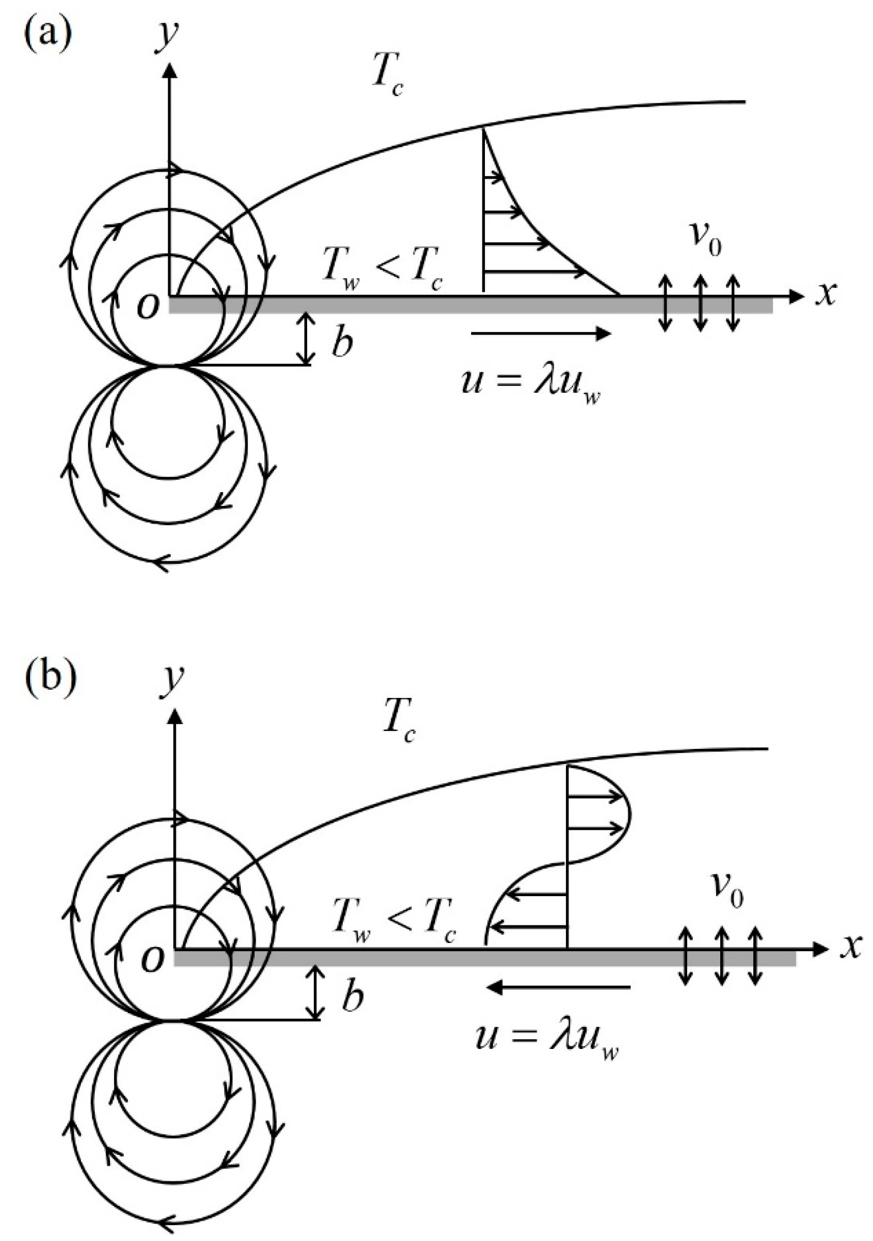
2. Mathematical Formulation

Figure 1 displays the physical model of the flow of a hybrid nanomaterial past a stretched and shrunken surface. Here, $v_0$ is the constant mass flux and $u_w(x)=ax$ is the surface velocity, where $a$ is a constant. The ambient temperature is considered to be at the temperature $T_{\infty }=T_c$ ($T_c$ is the Curie temperature), while the surface temperature $T_w$ is kept constant such that $T_w<T_c$. The nanoparticles have a uniform spherical shape, and their size remains consistent. Additionally, the composite nature of the stable hybrid nanofluids ensures that any agglomeration effects are disregarded.

Therefore, the governing equations are (see [27,46,59])

$$\frac{\partial u}{\partial x}+\frac{\partial v}{\partial y}=0$$

(1)

$$u\frac{\partial u}{\partial x}+v\frac{\partial u}{\partial y}=\frac{{\mu }_{hnf}}{{\rho }_{hnf}}\frac{{\partial }^{2}u}{\partial y^2}+\frac{{\mu }_0}{{\rho }_{hnf}}M\frac{\partial H}{\partial x}$$

(2)

$$u\frac{\partial T}{\partial x}+v\frac{\partial T}{\partial y}+\frac{{\mu }_0}{{(\rho C_p)}_{hnf}}T\frac{\partial M}{\partial T}\left(u\frac{\partial H}{\partial x}+v\frac{\partial H}{\partial y}\right)=\frac{k_{hnf}}{{(\rho C_p)}_{hnf}}\frac{{\partial }^{2}T}{\partial y^2}-\frac{1}{{(\rho C_p)}_{hnf}}\frac{\partial q_r}{\partial y}$$

(3)

subject to the following:

$$\begin{array}{l}v=v_0,\hspace{0.17em}\hspace{0.17em}\hspace{0.17em}\hspace{0.17em}\hspace{0.17em}\hspace{0.17em}\hspace{0.17em}u=\lambda u_w,\hspace{0.17em}\hspace{0.17em}\hspace{0.17em}\hspace{0.17em}\hspace{0.17em}\hspace{0.17em}\hspace{0.17em}T=T_w\hspace{0.17em}\hspace{0.17em}\hspace{0.17em}\hspace{0.17em}\hspace{0.17em}\hspace{0.17em}\hspace{0.17em}\hspace{0.17em}\hspace{0.17em}\hspace{0.17em}\hspace{0.17em}\hspace{0.17em}\mathrm{at}\hspace{0.17em}\hspace{0.17em}\hspace{0.17em}\hspace{0.17em}\hspace{0.17em}\hspace{0.17em}\hspace{0.17em}\hspace{0.17em}\hspace{0.17em}\hspace{0.17em}\hspace{0.17em}\hspace{0.17em}y=0\\ u\to 0,\hspace{0.17em}\hspace{0.17em}\hspace{0.17em}\hspace{0.17em}\hspace{0.17em}\hspace{0.17em}\hspace{0.17em}T\to T_c\hspace{0.17em}\hspace{0.17em}\hspace{0.17em}\hspace{0.17em}\hspace{0.17em}\hspace{0.17em}\hspace{0.17em}\hspace{0.17em}\hspace{0.17em}\hspace{0.17em}\mathrm{as}\hspace{0.17em}\hspace{0.17em}\hspace{0.17em}\hspace{0.17em}\hspace{0.17em}\hspace{0.17em}\hspace{0.17em}\hspace{0.17em}\hspace{0.17em}\hspace{0.17em}\hspace{0.17em}y\to \infty \end{array}$$

(4)

where the velocity components along the x- and y-axes are represented by u and v, while $T$, $M$, ${\mu }_0$, $H$, and $q_r$ indicate the hybrid nanofluid temperature, magnetization, magnetic permeability, magnetic field, and radiative heat flux, respectively. Further, $\lambda$ represents the stretching/shrinking parameter, with $\lambda >0$ and $\lambda <0$ for stretched and shrunken surfaces, respectively, while the static sheet is denoted by $\lambda =0$.

By means of Rosseland’s [60] approximation, the expression of the radiative heat flux is given as (see [61,62])

$$q_r=-\frac{4{\sigma }^{\ast }}{3k^{\ast }}\frac{\partial T^4}{\partial y}$$

(5)

where $k^{\ast }$ and ${\sigma }^{\ast }$ denote the mean absorption coefficient and the Stefan–Boltzmann constant, respectively. By using the Taylor series, $T^4$ is expanded about $T_c$, and by ignoring the terms of the higher order, we obtain

$$T^4\cong 4T_c^{3}T-3T_c^4$$

(6)

Using (5) and (6), Equation (3) can be written as follows:

$$u\frac{\partial T}{\partial x}+v\frac{\partial T}{\partial y}+\frac{{\mu }_0}{{(\rho C_p)}_{hnf}}T\frac{\partial M}{\partial T}\left(u\frac{\partial H}{\partial x}+v\frac{\partial H}{\partial y}\right)=\frac{1}{{(\rho C_p)}_{hnf}}\left(k_{hnf}+\frac{16{\sigma }^{\ast }{T}_{\infty }^3}{3k^{\ast }}\right)\frac{{\partial }^{2}T}{\partial y^2}$$

(7)

Further, ${(\rho C_p)}_{hnf},\hspace{0.17em}\hspace{0.17em}{k}_{hnf},\hspace{0.17em}\hspace{0.17em}{\mu }_{hnf},$ and ${\rho }_{hnf}$ characterize the heat capacity, thermal conductivity, dynamic viscosity, and density of the hybrid nanofluid, respectively, where their thermophysical properties are defined in

Table 1. Thermophysical properties of nanofluid and hybrid nanofluid.

Thermophysical Properties	Nanofluid	Hybrid Nanofluid
Dynamic viscosity	${\mu }_{nf}=\frac{{\mu }_f}{{(1-{\phi }_1)}^{2.5}}$	${\mu }_{hnf}=\frac{{\mu }_f}{{(1-{\phi }_1)}^{2.5}{(1-{\phi }_2)}^{2.5}}$
Heat capacity	$\begin{array}{c}{(\rho C_p)}_{nf}=(1-{\phi }_1){(\rho C_p)}_f\\ +{\phi }_1{(\rho C_p)}_{n1}\end{array}$	$\begin{array}{ll}{(\rho C_p)}_{hnf}=& (1-{\phi }_2)[(1-{\phi }_1){(\rho C_p)}_f+{\phi }_1{(\rho C_p)}_{n1}]\\ & +{\phi }_2{(\rho C_p)}_{n2}\end{array}$
Density	${\rho }_{nf}=(1-{\phi }_1){\rho }_f+{\phi }_1{\rho }_{n1}$	${\rho }_{hnf}=(1-{\phi }_2)[(1-{\phi }_1){\rho }_f+{\phi }_1{\rho }_{n1}]+{\phi }_2{\rho }_{n2}$
Thermal conductivity	$k_{nf}=\frac{k_{n1}+2k_f-2{\phi }_1(k_f-k_{n1})}{k_{n1}+2k_f+{\phi }_1(k_f-k_{n1})}\times (k_f)$	$k_{hnf}=\frac{k_{n2}+2k_{nf}-2{\phi }_2(k_{nf}-k_{n2})}{k_{n2}+2k_{nf}+{\phi }_2(k_{nf}-k_{n2})}\times (k_{nf})$ where $k_{nf}=\frac{k_{n1}+2k_f-2{\phi }_1(k_f-k_{n1})}{k_{n1}+2k_f+{\phi }_1(k_f-k_{n1})}\times (k_f)$

(see [3,27,31]). Meanwhile, the physical properties of Cu, Al₂O₃, and water are given in

Table 2. Thermophysical properties of nanoparticles and water.

Thermophysical Properties	$\mathbf{Cu} \left({\mathit{\phi }}_1\right)$	${\mathbf{Al}}_2{\mathbf{O}}_3 \left({\mathit{\phi }}_2\right)$	Water
$k\hspace{0.17em}(\mathrm{W}/\mathrm{mK})$	400	40	0.613
$C_p\hspace{0.17em}(\mathrm{J}/\mathrm{kgK})$	385	765	4179
$\rho \hspace{0.17em}{(\mathrm{kg}/\mathrm{m}}^3)$	8933	3970	997.1
Prandtl number, $\mathrm{Pr}$			6.2

(see [3,31]). Here, $k,\hspace{0.17em}\hspace{0.17em}\rho ,\hspace{0.17em}\hspace{0.17em}\mu ,\hspace{0.17em}\hspace{0.17em}(\rho C_p),$ and $C_p$ represent the thermal conductivity, density, dynamic viscosity, heat capacity, and specific heat at constant pressure, respectively.

As stated in the studies by Neuringer [45] and Andersson and Valnes [46], the scalar magnetic potential is defined as follows:

$$\mathsf{\Phi }=\frac{\delta }{2\pi }\frac{x}{x^2+{(y+d)}^2}$$

(8)

where $\delta$ denotes the magnetic field strength and $d$ indicates the distance of the center of the magnetic dipole from the origin. The component’s form of the scalar magnetic potential can be written as

$$H_x=-\frac{\partial \mathsf{\Phi }}{\partial x}=\frac{\delta }{2\pi }\frac{x^2-{(y+d)}^2}{{\left[x^2+{(y+d)}^2\right]}^2}$$

(9)

$$H_y=-\frac{\partial \mathsf{\Phi }}{\partial x}=\frac{\delta }{2\pi }\frac{2x(y+d)}{{\left[x^2+{(y+d)}^2\right]}^2}$$

(10)

The magnitude of the magnetic field $H$ is

$$H={\left[{\left(\frac{\partial \mathsf{\Phi }}{\partial x}\right)}^2+{\left(\frac{\partial \mathsf{\Phi }}{\partial y}\right)}^2\right]}^{1/2}$$

(11)

From (9) and (10), we can write

$$\frac{\partial H}{\partial x}=-\frac{\delta }{2\pi }\frac{2x}{{(y+d)}^4}$$

(12)

$$\frac{\partial H}{\partial y}=-\frac{\delta }{2\pi }\left[\frac{2}{{(y+d)}^3}-\frac{4x^2}{{(y+d)}^5}\right]$$

(13)

The relation between the temperature $T$ and the magnetization $M$ with the constant pyromagnetic coefficient $K$ is given by

$$M=K(T_c-T)$$

(14)

An appropriate transformation is introduced as follows (see [53,55,59]):

$$\psi (\xi ,\eta )=\nu {}_f\xi f(\eta ),\hspace{0.17em}\hspace{0.17em}\hspace{0.17em}\hspace{0.17em}\hspace{0.17em}\hspace{0.17em}\hspace{0.17em}\theta (\eta )=\frac{T_c-T}{T_c-T_w},\hspace{0.17em}\hspace{0.17em}\hspace{0.17em}\hspace{0.17em}\hspace{0.17em}\hspace{0.17em}\eta =y\sqrt{\frac{a}{\nu {}_f}},\hspace{0.17em}\hspace{0.17em}\hspace{0.17em}\hspace{0.17em}\hspace{0.17em}\hspace{0.17em}\xi =x\sqrt{\frac{a}{\nu {}_f}}$$

(15)

where $\xi$ and $\eta$ are the dimensionless coordinates, and $\nu {}_f$ is the fluid’s kinematic viscosity. Here, $\psi$ denotes the stream function with $u=\partial \psi /\partial y$ and $v=-\partial \psi /\partial x$ so that Equation (1) is identically fulfilled. Employing these definitions, we obtain

$$u=ax{f}^{\prime }(\eta ),\hspace{0.17em}\hspace{0.17em}\hspace{0.17em}\hspace{0.17em}\hspace{0.17em}v=-\sqrt{a{v}_f}f(\eta )$$

(16)

so that

$$v_0=-\sqrt{a{v}_f}S$$

(17)

Using (15), Equations (2) and (7) are transformed to the following:

$$\frac{{\mu }_{hnf}/{\mu }_f}{{\rho }_{hnf}/{\rho }_f}{f}^{‴}+f{f}^{″}-{f^{\prime }}^2-\frac{1}{{\rho }_{hnf}/{\rho }_f}\frac{2}{{(\eta +\alpha )}^4}\beta \theta =0$$

(18)

$$\begin{array}{l}\frac{1}{\mathrm{Pr}}\frac{1}{{(\rho C_p)}_{hnf}/{(\rho C_p)}_f}\left[\left(\frac{k_{hnf}}{k_f}+\frac{4}{3}R\right){\theta }^{″}+\frac{2}{{(\eta +\alpha )}^3}\beta {\lambda }_1(\theta -\epsilon )f\right]+f{\theta }^{\prime }\\ \hspace{0.17em}\hspace{0.17em}\hspace{0.17em}\hspace{0.17em}\hspace{0.17em}\hspace{0.17em}\hspace{0.17em}\hspace{0.17em}\hspace{0.17em}\hspace{0.17em}\hspace{0.17em}\hspace{0.17em}\hspace{0.17em}\hspace{0.17em}\hspace{0.17em}\hspace{0.17em}\hspace{0.17em}+{\xi }^2\left[\frac{1}{\mathrm{Pr}}\frac{1}{{(\rho C_p)}_{hnf}/{(\rho C_p)}_f}\beta {\lambda }_1\left(-\frac{2}{{(\eta +\alpha )}^4}{f}^{\prime }-\frac{2}{{(\eta +\alpha )}^5}f\right)(\theta -\epsilon )\right]=0\end{array}$$

(19)

However, by considering the similarity equations, the coefficient for ${\xi }^2$ in Equation (19) is negligible. It is to reduce the complexity of equations where the model will be deduced to the similarity equations where there is only an independent variable that exists in the final equations. This approach is also pondered by Hayat et al. [53], Nadeem et al. [55], and Yasmeen et al. [59]. Therefore, we have

$$\frac{1}{\mathrm{Pr}}\frac{1}{{(\rho C_p)}_{hnf}/{(\rho C_p)}_f}\left[\left(\frac{k_{hnf}}{k_f}+\frac{4}{3}R\right){\theta }^{″}+\frac{2}{{(\eta +\alpha )}^3}\beta {\lambda }_1(\theta -\epsilon )f\right]+f{\theta }^{\prime }=0$$

(20)

which is subject to

$$\begin{array}{l}f(0)=S,\hspace{0.17em}\hspace{0.17em}\hspace{0.17em}\hspace{0.17em}\hspace{0.17em}\hspace{0.17em}\hspace{0.17em}\hspace{0.17em}{f}^{\prime }(0)=\lambda ,\hspace{0.17em}\hspace{0.17em}\hspace{0.17em}\hspace{0.17em}\hspace{0.17em}\hspace{0.17em}\hspace{0.17em}\theta (0)=1\\ f^{\prime }(\eta )\to 0,\hspace{0.17em}\hspace{0.17em}\hspace{0.17em}\hspace{0.17em}\hspace{0.17em}\hspace{0.17em}\theta (\eta )\to 0\hspace{0.17em}\hspace{0.17em}\hspace{0.17em}\hspace{0.17em}\hspace{0.17em}\hspace{0.17em}\hspace{0.17em}\hspace{0.17em}\hspace{0.17em}\hspace{0.17em}\mathrm{as}\hspace{0.17em}\hspace{0.17em}\hspace{0.17em}\hspace{0.17em}\hspace{0.17em}\hspace{0.17em}\hspace{0.17em}\eta \to \infty \end{array}$$

(21)

Here, $S=f(0)$ is the mass flux parameter, where suction and injection (blowing) are denoted by $S>0$ and $S<0$, respectively, while the primes indicate the differentiation with respect to $\eta$. Further, $\mathrm{Pr}$, $R$, $\beta$, ${\lambda }_1$, $\alpha$, and $\epsilon$ represent the Prandtl number, the radiation, the ferrohydrodynamic interaction, the viscous dissipation, the dimensionless distance, and the dimensionless temperature parameters, respectively, which are expressed as

$$\begin{array}{l}\mathrm{Pr}=\frac{{(\mu C_p)}_f}{k_f},\hspace{0.17em}\hspace{0.17em}\hspace{0.17em}\hspace{0.17em}\hspace{0.17em}R=\frac{4{\sigma }^{\ast }{T}_c{}^3}{k^{\ast }{k}_f},\hspace{0.17em}\hspace{0.17em}\hspace{0.17em}\hspace{0.17em}\hspace{0.17em}\beta =\frac{\delta {\rho }_f{\mu }_{0}K(T_c-T_w)}{2\pi {\mu }_f{}^2},\\ {\lambda }_1=\frac{a{\mu }_f{}^2}{{\rho }_f{k}_f(T_c-T_w)},\hspace{0.17em}\hspace{0.17em}\hspace{0.17em}\hspace{0.17em}\hspace{0.17em}\alpha =d\sqrt{\frac{a}{\nu {}_f}},\hspace{0.17em}\hspace{0.17em}\hspace{0.17em}\hspace{0.17em}\hspace{0.17em}\hspace{0.17em}\epsilon =\frac{T_c}{T_c-T_w}\end{array}$$

(22)

The local Nusselt number $N{u}_x$ and the skin friction coefficient $C_f$ are given as

$$N{u}_x=-\frac{x{q}_w}{k_f(T_c-T_w)},\hspace{0.17em}\hspace{0.17em}\hspace{0.17em}\hspace{0.17em}\hspace{0.17em}\hspace{0.17em}\hspace{0.17em}\hspace{0.17em}\hspace{0.17em}\hspace{0.17em}\hspace{0.17em}\hspace{0.17em}\hspace{0.17em}\hspace{0.17em}{C}_f=\frac{{\tau }_w}{{\rho }_f{u}_w{}^2}$$

(23)

where the surface heat flux $q_w$ and the surface shear stress ${\tau }_w$ are defined by

$$q_w=-k_{hnf}{\left(\frac{\partial T}{\partial y}\right)}_{y=0}+{\left(q_r\right)}_{y=0},\hspace{0.17em}\hspace{0.17em}\hspace{0.17em}\hspace{0.17em}\hspace{0.17em}\hspace{0.17em}\hspace{0.17em}\hspace{0.17em}\hspace{0.17em}\hspace{0.17em}\hspace{0.17em}\hspace{0.17em}\hspace{0.17em}{\tau }_w={\mu }_{hnf}{\left(\frac{\partial u}{\partial y}\right)}_{y=0}$$

(24)

Employing (15), (23), and (24), we have

$${\mathrm{Re}}_x^{-1/2}N{u}_x=-\left(\frac{k_{hnf}}{k_f}+\frac{4}{3}R\right){\theta }^{\prime }(0),\hspace{0.17em}\hspace{0.17em}\hspace{0.17em}\hspace{0.17em}\hspace{0.17em}\hspace{0.17em}\hspace{0.17em}\hspace{0.17em}\hspace{0.17em}\hspace{0.17em}\hspace{0.17em}\hspace{0.17em}\hspace{0.17em}\hspace{0.17em}{\mathrm{Re}}_x^{1/2}{C}_f=\frac{{\mu }_{hnf}}{{\mu }_f}{f}^{″}(0)$$

(25)

where ${\mathrm{Re}}_x=u_{w}x/{\nu }_f$ denotes the local Reynolds number.

3. Stability Analysis

The existence of the non-uniqueness solutions from Equations (18), (20), and (21) are observed for a certain value of the physical parameters. A temporal stability analysis is therefore needed to ensure which solutions are stable (see Merkin [63] and Weidman et al. [64]). Therefore, the new variables based on Equation (15) are given as follows:

$$\psi (\xi ,\eta ,\tau )=\nu {}_f\xi f(\eta ,\tau ),\hspace{0.17em}\hspace{0.17em}\hspace{0.17em}\hspace{0.17em}\hspace{0.17em}\hspace{0.17em}\hspace{0.17em}\theta (\eta ,\tau )=\frac{T_c-T}{T_c-T_w},\hspace{0.17em}\hspace{0.17em}\hspace{0.17em}\hspace{0.17em}\hspace{0.17em}\hspace{0.17em}\eta =y\sqrt{\frac{a}{\nu {}_f}},\hspace{0.17em}\hspace{0.17em}\hspace{0.17em}\hspace{0.17em}\hspace{0.17em}\hspace{0.17em}\xi =x\sqrt{\frac{a}{\nu {}_f}},\hspace{0.17em}\hspace{0.17em}\hspace{0.17em}\hspace{0.17em}\hspace{0.17em}\hspace{0.17em}\tau =at$$

(26)

The unsteady form of Equations (1)–(3) are considered to analyze the stability of their solutions. By using (26), we obtain the following:

$$\frac{{\mu }_{hnf}/{\mu }_f}{{\rho }_{hnf}/{\rho }_f}\frac{{\partial }^{3}f}{\partial {\eta }^3}+f\frac{{\partial }^{2}f}{\partial {\eta }^2}-{\left(\frac{\partial f}{\partial \eta }\right)}^2-\frac{1}{{\rho }_{hnf}/{\rho }_f}\frac{2}{{(\eta +\alpha )}^4}\beta \theta -\frac{{\partial }^{2}f}{\partial \eta \partial \tau }=0$$

(27)

$$\frac{1}{\mathrm{Pr}}\frac{1}{{(\rho C_p)}_{hnf}/{(\rho C_p)}_f}\left[\left(\frac{k_{hnf}}{k_f}+\frac{4}{3}R\right)\frac{{\partial }^2\theta }{\partial {\eta }^2}+\frac{2}{{(\eta +\alpha )}^3}\beta {\lambda }_1(\theta -\epsilon )f\right]+f\frac{\partial \theta }{\partial \eta }-\frac{\partial \theta }{\partial \tau }=0$$

(28)

which is subject to

$$\begin{array}{l}f(0,\tau )=S,\hspace{0.17em}\hspace{0.17em}\hspace{0.17em}\hspace{0.17em}\hspace{0.17em}\hspace{0.17em}\hspace{0.17em}\hspace{0.17em}\frac{\partial f}{\partial \eta }(0,\tau )=\lambda ,\hspace{0.17em}\hspace{0.17em}\hspace{0.17em}\hspace{0.17em}\hspace{0.17em}\hspace{0.17em}\hspace{0.17em}\hspace{0.17em}\hspace{0.17em}\theta (0,\tau )=1\\ \frac{\partial f}{\partial \eta }(\eta ,\tau )\to 0,\hspace{0.17em}\hspace{0.17em}\hspace{0.17em}\hspace{0.17em}\hspace{0.17em}\hspace{0.17em}\theta (\eta ,\tau )\to 0\hspace{0.17em}\hspace{0.17em}\hspace{0.17em}\hspace{0.17em}\hspace{0.17em}\hspace{0.17em}\hspace{0.17em}\hspace{0.17em}\hspace{0.17em}\hspace{0.17em}\hspace{0.17em}\hspace{0.17em}\mathrm{as}\hspace{0.17em}\hspace{0.17em}\hspace{0.17em}\hspace{0.17em}\hspace{0.17em}\hspace{0.17em}\hspace{0.17em}\eta \to \infty \end{array}$$

(29)

To examine the stability behavior, the disturbance is imposed to the steady solution $f=f_0(\eta )$ and $\theta ={\theta }_0(\eta )$ of Equations (18), (20), and (21) by using the following relations (see [64]):

$$f(\eta ,\tau )=f_0(\eta )+e^{-\gamma \tau }F(\eta ),\hspace{0.17em}\hspace{0.17em}\hspace{0.17em}\hspace{0.17em}\hspace{0.17em}\hspace{0.17em}\hspace{0.17em}\hspace{0.17em}\hspace{0.17em}\hspace{0.17em}\hspace{0.17em}\hspace{0.17em}\hspace{0.17em}\hspace{0.17em}\hspace{0.17em}\theta (\eta ,\tau )={\theta }_0(\eta )+e^{-\gamma \tau }G(\eta )$$

(30)

where $\gamma$ indicates the unknown eigenvalue, which determines the stability of the solutions, whereas $F(\eta )$ and $G(\eta )$ are comparatively small to $f_0(\eta )$ and ${\theta }_0(\eta )$. The disturbance is taken exponentially as it demonstrates the rapid decline or development of the disturbance. By inserting Equation (30) into Equations (27)–(29), we obtain the following:

$$\frac{{\mu }_{hnf}/{\mu }_f}{{\rho }_{hnf}/{\rho }_f}{F}^{‴}+f_0{F}^{″}+{f^{″}}_0\hspace{0.17em}F-2{f^{\prime }}_0{F}^{\prime }-\frac{1}{{\rho }_{hnf}/{\rho }_f}\frac{2}{{(\eta +\alpha )}^4}\beta G+\gamma F^{\prime }=0$$

(31)

$$\frac{1}{\mathrm{Pr}}\frac{1}{{(\rho C_p)}_{hnf}/{(\rho C_p)}_f}\left[\left(\frac{k_{hnf}}{k_f}+\frac{4}{3}R\right)G^{″}+\frac{2}{{(\eta +\alpha )}^3}\beta {\lambda }_1(f_{0}G+{\theta }_{0}F-\epsilon F)\right]\hspace{0.17em}+\hspace{0.17em}{f}_0{G}^{\prime }+{{\theta }^{\prime }}_{0}F+\gamma G=0$$

(32)

subject to

$$\begin{array}{l}F(0)=0,\hspace{0.17em}\hspace{0.17em}\hspace{0.17em}\hspace{0.17em}\hspace{0.17em}\hspace{0.17em}\hspace{0.17em}\hspace{0.17em}\hspace{0.17em}{F}^{\prime }(0)=0,\hspace{0.17em}\hspace{0.17em}\hspace{0.17em}\hspace{0.17em}\hspace{0.17em}\hspace{0.17em}\hspace{0.17em}\hspace{0.17em}\hspace{0.17em}G(0)=0\\ F^{\prime }(\eta )\to 0,\hspace{0.17em}\hspace{0.17em}\hspace{0.17em}\hspace{0.17em}\hspace{0.17em}\hspace{0.17em}\hspace{0.17em}\hspace{0.17em}G(\eta )\to 0\hspace{0.17em}\hspace{0.17em}\hspace{0.17em}\hspace{0.17em}\hspace{0.17em}\hspace{0.17em}\hspace{0.17em}\hspace{0.17em}\hspace{0.17em}\hspace{0.17em}\mathrm{as}\hspace{0.17em}\hspace{0.17em}\hspace{0.17em}\hspace{0.17em}\hspace{0.17em}\hspace{0.17em}\hspace{0.17em}\hspace{0.17em}\hspace{0.17em}\hspace{0.17em}\hspace{0.17em}\eta \to \infty \end{array}$$

(33)

Without the loss of generality, the values of $\gamma$ from Equations (31)–(33) are obtained for the case of $F^{″}(0)=1$, as discussed by Harris et al. [65].

4. Results and Discussion

This section is divided into two parts, the computational approach and the results analysis.

4.1. Computational Approach

The bvp4c solver in Matlab software is utilized for evaluating Equations (18), (20), and (21) numerically. Following the methodology outlined in Shampine et al. [66], the aforementioned solver utilizes a finite difference approach based on the three-stage Lobatto IIIa formula. In the present study, we consider the volume fractions of Cu, which varies from 0 to 0.06 $(0\le {\phi }_2\le 0.06)$, while the volume fraction of Al₂O₃ is maintained at ${\phi }_1=0.1$, and water is used as a base fluid. We note from Equations (18) and (20) that the parameters ${\lambda }_1$, $\alpha$, and $\epsilon$ depend on $\beta$. In the absence of ferrohydrodynamic interaction $(\beta =0)$, these three parameters do not affect the equations. Thus, for general cases, when $\beta \ne 0$, we fix the values of these parameters as ${\lambda }_1=0.01$, $\alpha =1$, and $\epsilon =2$, as suggested by Neuringer [45] and Andersson and Valnes [46]. Since we want to highlight the availability of dual solutions for the shrinking flow case, we only focus on certain values of the controlling parameters. Additionally, the critical values of the parameters are examined. However, there is no restriction if other researchers want to use other values, but the availability of the second solution may be affected, as well as the existence of the similarity solutions.

The numerical procedures can be described as follows. Firstly, Equations (18) and (20) are transformed into a system of first-order ordinary differential equations.

Thus, Equation (18) can be written as follows:

$$f=y\left(1\right) ,$$

$$f^{\prime }=y^{\prime }\left(1\right)=y\left(2\right) ,$$

(34a)

$$f^{″}=y^{\prime }\left(2\right)=y\left(3\right) ,$$

(34b)

$$f^{‴}=y’\left(3\right)=-\frac{{\rho }_{hnf}/{\rho }_f}{{\mu }_{hnf}/{\mu }_f}\left(y\left(1\right)y\left(3\right)-y{\left(2\right)}^2-\frac{1}{{\rho }_{hnf}/{\rho }_f}\frac{2}{{\left(\eta +\alpha \right)}^4}\beta \theta \right) ,$$

(34c)

while Equation (20) reduces to

$$\theta =y\left(4\right) ,$$

$${\theta }^{\prime }=y^{\prime }\left(4\right)=y\left(5\right) ,$$

(35a)

$${\theta }^{″}=y^{\prime }\left(5\right)=-{\left[\frac{k_{hnf}}{k_f }+\frac{4}{3 }R\right]}^{-1}\left[\frac{2}{{\left(\eta +\alpha \right)}^3}\beta {\lambda }_1\left(\theta -\epsilon \right)y\left(1\right)+\mathrm{Pr}\frac{{\left(\rho C_p\right)}_{hnf}}{{\left(\rho C_p\right)}_f }y\left(1\right)y\left(5\right)\right] ,$$

(35b)

and the boundary condition (21) becomes

$$y_a\left(1\right)=S, y_a\left(2\right)=\lambda , y_a\left(4\right)=1,$$

$$y_b\left(2\right)⟶1, y_b\left(4\right)⟶0 .$$

(36)

The subscript ‘a’ represents the condition at the surface, while the subscript ‘b’ represents the condition at the free stream. Subsequently, Equations (34)–(36) are implemented in the Matlab software and solved using the bvp4c solver. The solver will be executed, generating numerical solutions and graphical outputs.

To guarantee the precision of the computation, the present results are validated using the existing data from the previous studies.

Table 3. Values of $-{\theta }^{\prime }(0)$ with different values of $\mathrm{Pr}$ when ${\phi }_1={\phi }_2=0$ (regular fluid), $\beta =S=R=0$, and $\lambda =1$ (stretching sheet).

Pr	Devi and Devi [27]	Waini et al. [31]	Khan and Pop [67]	Hamad [68]	Present Results
2	0.91135	0.911353	0.9113	0.91136	0.91136
6.2	-	-	-	-	1.77095
7	1.89540	1.895400	1.8954	1.89540	1.89540
20	3.35390	3.353902	3.3539	3.35390	3.35390

provides the comparison values of $-{\theta }^{\prime }(0)$ with different values of $\mathrm{Pr}$ when ${\phi }_1={\phi }_2=0$ (regular fluid), $\beta =S=R=0$, and $\lambda =1$ (stretching sheet). The present results are comparable with those obtained by Devi and Devi [27], Waini et al. [31], Khan and Pop [67], and Hamad [68], for each value of $\mathrm{Pr}$ considered.

Other than that,

Table 4. Values of $-f^{″}(0)$ and $-{\theta }^{\prime }(0)$ with different values of ${\phi }_2$ when $\beta =S=R=0$ and $\lambda =1$ (stretching sheet) for Cu-water nanofluid (${\phi }_1=0$ ).

${\mathit{\phi }}_2$	$-{\mathit{f}}^{″}(0)$			$-{\mathit{\theta }}^{\prime }(0)$
	Waini et al. [69]	Hamad [68]	Present Results	Hamad [68]	Present Results
0.05	1.10892	1.10892	1.10892	1.59899	1.59899
0.1	1.17475	1.17475	1.17475	1.45207	1.45207
0.15	1.20886	1.20886	1.20886	1.32465	1.32465
0.2	1.21804	1.21804	1.21804	1.21290	1.21290

presents the comparison values of $-f^{″}(0)$ and $-{\theta }^{\prime }(0)$ for Cu-water nanofluid (${\phi }_1=0$) under different values of ${\phi }_2$ with Waini et al. [69] and Hamad [68]. The comparison is performed by taking $\beta =S=R=0$ and $\lambda =1$ (stretching sheet), and it shows an excellent agreement between those results.

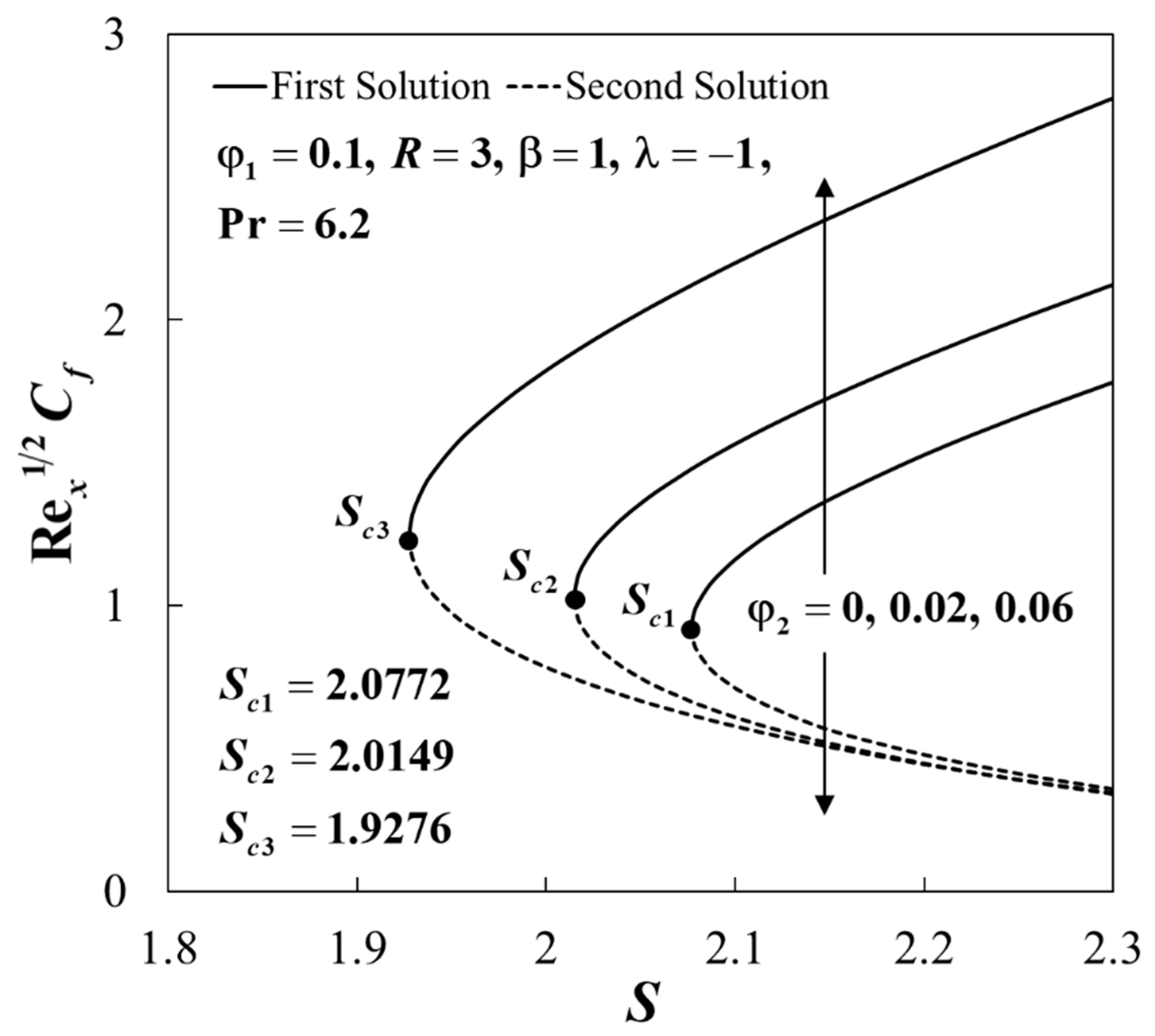
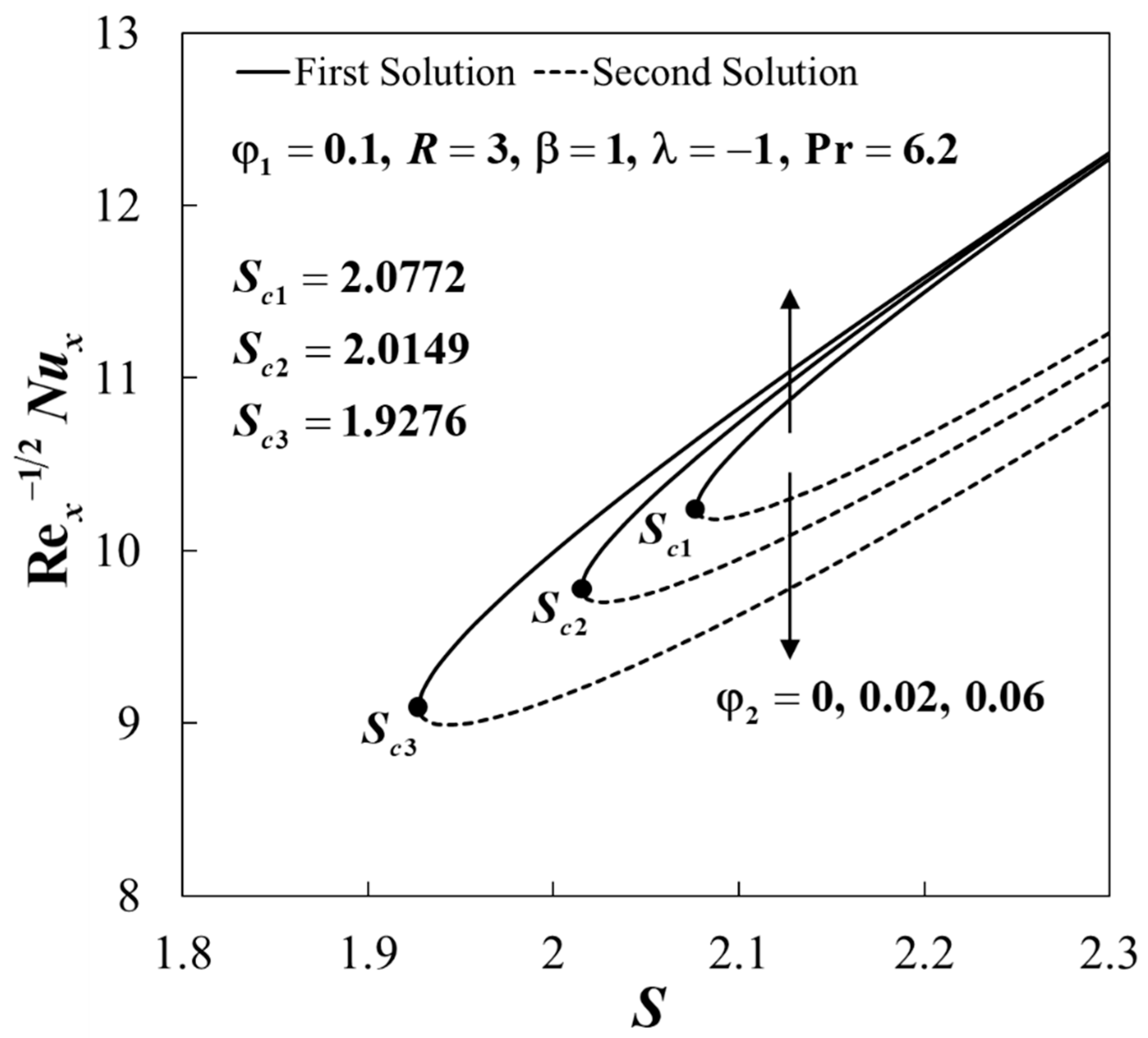
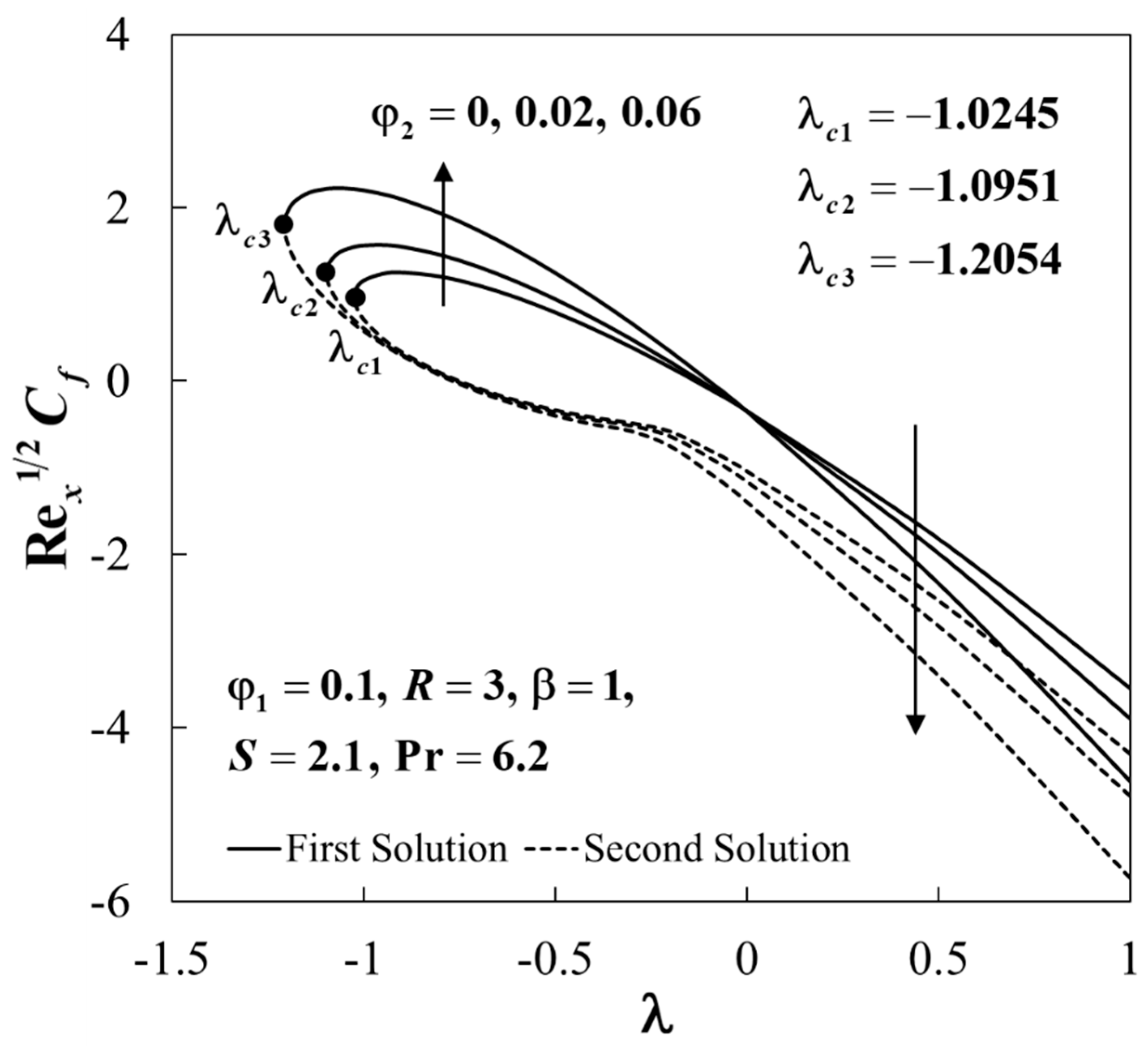
4.2. Results Analysis

The values of the skin friction coefficient ${\mathrm{Re}}_x^{1/2}{C}_f$ and the local Nusselt number ${\mathrm{Re}}_x^{-1/2}N{u}_x$ for the nanofluid (Cu/water) and hybrid nanofluid (Cu-Al₂O₃/water) when $S=0$, $\lambda =1$ (stretching sheet), and $\mathrm{Pr}=6.2$ under different physical parameters are presented in

Table 5. Values of ${\mathrm{Re}}_x^{1/2}{C}_f$ and ${\mathrm{Re}}_x^{-1/2}N{u}_x$ for Cu/water nanofluid $({\phi }_1=0)$ and Cu-Al₂O₃/water hybrid nanofluid $({\phi }_1=0.1)$ when $S=0$, $\lambda =1$ (stretching sheet), and $\mathrm{Pr}=6.2$ under different physical parameters.

${\mathit{\phi }}_2$	$\mathit{\beta }$	$\mathit{R}$	$\mathbf{Cu}/\mathbf{Water} ({\mathit{\phi }}_1=0)$ (Nanofluid)		$\mathbf{Cu}-{\mathbf{Al}}_2{\mathbf{O}}_3/\mathbf{Water} ({\mathit{\phi }}_1=0.1)$ (Hybrid Nanofluid)
			${\mathbf{Re}}_{\mathit{x}}^{1/2}{\mathit{C}}_{\mathit{f}}$	${\mathbf{Re}}_{\mathit{x}}^{-1/2}\mathit{N}{\mathit{u}}_{\mathit{x}}$	${\mathbf{Re}}_{\mathit{x}}^{1/2}{\mathit{C}}_{\mathit{f}}$	${\mathbf{Re}}_{\mathit{x}}^{-1/2}\mathit{N}{\mathit{u}}_{\mathit{x}}$
0	0	0	−1.00000	1.77095	−1.29975	1.96441
0.02	0	0	−1.10419	1.80221	−1.40946	2.00140
0.04	0	0	−1.20831	1.83408	−1.52069	2.03888
0.06	0	0	−1.31329	1.86658	−1.63408	2.07693
0.02	0.5	0	−1.24681	1.78936	−1.56126	1.98814
0.02	1	0	−1.39058	1.77601	−1.71411	1.97443
0.02	2	0	−1.68191	1.74768	−2.02320	1.94549
0.02	3	0	−1.97900	1.71678	−2.33737	1.91423
0.02	1	0.5	−1.41962	2.16737	−1.73651	2.30785
0.02	1	1	−1.43792	2.45694	−1.75163	2.56590
0.02	1	2	−1.46084	2.87521	−1.77150	2.95160
0.02	1	3	−1.47519	3.17146	−1.78439	3.23279

. The values of ${\mathrm{Re}}_x^{-1/2}N{u}_x$ accelerate with the rising values of ${\phi }_2$ and $R$ for both the nanofluid and hybrid nanofluid, whereas it decelerates with the increase in $\beta$. However, the rise in ${\phi }_2$, $\beta$, and $R$ tend to decrease the values of ${\mathrm{Re}}_x^{1/2}{C}_f$. The values of ${\mathrm{Re}}_x^{-1/2}N{u}_x$ are enhanced with the rise in ${\phi }_2$, but it is intensified for hybrid nanofluid, which proves that the heat transfer rate is increased by the hybrid nanoparticles. It is observed that the heat transfer rate is increased by 10.92% for the nanofluid, with a 15.13% increment for the hybrid nanofluid compared to the base fluid.

The variations of ${\mathrm{Re}}_x^{1/2}{C}_f$ and ${\mathrm{Re}}_x^{-1/2}N{u}_x$ against $\lambda$ and $S$ for several physical parameters are presented in Figure 2, Figure 3, Figure 4, Figure 5, Figure 6, Figure 7, Figure 8 and Figure 9.

The non-uniqueness of the solutions for Equations (9)–(11) are observed when $S>S_c$ and $\lambda >{\lambda }_c$. Meanwhile, for $S<S_c$ and $\lambda <{\lambda }_c$, there are no similar solutions obtained as a consequence of the boundary layer separation. The variations of ${\mathrm{Re}}_x^{1/2}{C}_f$ and ${\mathrm{Re}}_x^{-1/2}N{u}_x$ for the shrinking sheet $(\lambda =-1)$ when ${\phi }_1=0.1,\hspace{0.17em}\hspace{0.17em}R=3,\hspace{0.17em}\hspace{0.17em}\beta =1$ and $\mathrm{Pr}=6.2$ with the effect of $S$ and ${\phi }_2$ are displayed in Figure 2 and Figure 3. For ${\phi }_2=0$, the dual solutions exist when $S_{c1}\ge 2.0772$, while for ${\phi }_2=0.02$, $S_{c2}\ge 2.0149$ and for ${\phi }_2=0.06$, $S_{c3}\ge 1.9276$. So, to obtain the solutions for a shrinking sheet, a satisfactory suction strength is required. Moreover, the values of ${\mathrm{Re}}_x^{1/2}{C}_f$ and ${\mathrm{Re}}_x^{-1/2}N{u}_x$ show the increasing behavior of the upper branch with an increase in ${\phi }_2$, but a decreasing behavior for the lower branch. This behavior is expected to occur because the addition of nanoparticles contributes to the enhancement of the thermal properties of fluids, which is due to the synergetic effects of the nanoparticles.

The plots of ${\mathrm{Re}}_x^{1/2}{C}_f$ and ${\mathrm{Re}}_x^{-1/2}N{u}_x$ against $\lambda$ for different values of ${\phi }_2$ when ${\phi }_1=0.1,\hspace{0.17em}\hspace{0.17em}R=3,$ $\beta =1,\hspace{0.17em}\hspace{0.17em}S=2.1,$ and $\mathrm{Pr}=6.2$ are illustrated in Figure 4 and Figure 5. Note that the lower branch solutions of ${\mathrm{Re}}_x^{1/2}{C}_f$ and ${\mathrm{Re}}_x^{-1/2}N{u}_x$ decrease with the rise in ${\phi }_2$. However, dual behaviors are observed for the upper branch where these values increase in the range where $\lambda$ is near to ${\lambda }_c$. Here, ${\lambda }_c=-1.0245$, $-1.0951$, and $-1.2054$ are the critical values for ${\phi }_2=0,\hspace{0.17em}0.02$ and $0.06$, respectively.

Additionally, Figure 6 and Figure 7 illustrate the role of $\beta$ against $\lambda$ on ${\mathrm{Re}}_x^{1/2}{C}_f$ and ${\mathrm{Re}}_x^{-1/2}N{u}_x$ when ${\phi }_1=0.1,\hspace{0.17em}\hspace{0.17em}{\phi }_2=0.02,$ $R=3,\hspace{0.17em}\hspace{0.17em}S=2.1,$ and $\mathrm{Pr}=6.2$. The rise in $\beta$ leads to the reduction in ${\mathrm{Re}}_x^{1/2}{C}_f$ and ${\mathrm{Re}}_x^{-1/2}N{u}_x$ for both branches. The domain of $\lambda$ is shortened where the critical value of $\lambda$ for $\beta =0,\hspace{0.17em}1$ and $2$ are ${\lambda }_c=-1.1690$, $-1.0951$, and $-1.0224$, respectively. The variations of ${\mathrm{Re}}_x^{1/2}{C}_f$ and ${\mathrm{Re}}_x^{-1/2}N{u}_x$ against $\lambda$ for different $R$ when ${\phi }_1=0.1,\hspace{0.17em}\hspace{0.17em}{\phi }_2=0.02,$ $\beta =1,\hspace{0.17em}\hspace{0.17em}S=2.1,$ and $\mathrm{Pr}=6.2$ are plotted in Figure 8 and Figure 9. The rise in $R$ has a tendency to decrease the values of ${\mathrm{Re}}_x^{1/2}{C}_f$ for both branches, as shown in Figure 8. Meanwhile, the upper branch solutions of the heat transfer rate ${\mathrm{Re}}_x^{-1/2}N{u}_x$ increase when $\lambda >0$ (stretching sheet), but it occurs almost at the same rate when $\lambda =0$ (static sheet), and decreases when $\lambda <0$ (shrinking sheet), as displayed in Figure 9. The critical value of $\lambda$ for $R=0,\hspace{0.17em}1$ and $3$ are ${\lambda }_c=-1.1573$, $-1.1361$, and $-1.0951$, respectively. The dominance of thermal radiation over conduction is shown by higher values of $R$. Consequently, a larger value of parameter R indicates an increased influx of radiative heat energy into the flow field, resulting in elevated temperatures. As a consequence, this leads to a decrease in the rate of heat transfer.

As seen in Figure 10, Figure 11, Figure 12, Figure 13, Figure 14 and Figure 15, the profiles of the velocity $f^{\prime }(\eta )$ and temperature $\theta (\eta )$ for both solutions are asymptotically satisfied with the free stream conditions (21). Therefore, the precision of the present results is reached. Figure 10 and Figure 11 show that the rise in ${\phi }_2$ leads to an increase in $f^{\prime }(\eta )$, but $\theta (\eta )$ decreases for the first solution, whereas the reverse behavior is seen for the lower branch when $\lambda =-1$ (shrinking sheet), ${\phi }_1=0.1,\hspace{0.17em}\hspace{0.17em}R=3,$ $\beta =1,\hspace{0.17em}\hspace{0.17em}S=2.1,$ and $\mathrm{Pr}=6.2$. The physical phenomena underlying these behaviors can be attributed to the introduction of nanoparticles, which increase the fluid’s viscosity, resulting in a deceleration of the flow and subsequently reduces the fluid velocity. Additionally, the presence of nanoparticles causes energy dissipation in the form of heat, leading to an elevation in the temperature. However, contrary to these expectations, this study observes opposite behaviors when the parameter ${\phi }_2$ is increased. This discrepancy is believed to be influenced by the shrinking of the sheet.

Moreover, Figure 12 and Figure 13 describe the behavior of $f^{\prime }(\eta )$ and $\theta (\eta )$ for different values of $\beta$ when $\lambda =-1$ (shrinking sheet), ${\phi }_1=0.1,\hspace{0.17em}\hspace{0.17em}{\phi }_2=0.02,$ $R=3,\hspace{0.17em}\hspace{0.17em}S=2.1,$ and $\mathrm{Pr}=6.2$. We notice that the upper branch solutions of $f^{\prime }(\eta )$ show a decreasing behavior with an increase in $\beta$, but it increases for the lower branch, as shown in Figure 12. However, the effect of $\beta$ is reversed on $\theta (\eta )$. From a physical perspective, the increase in parameter $\beta$ generates resistance forces within the flow, resulting in a deviation in the Lorentz force. This elevated resistance contributes to an increase in the fluid viscosity, consequently reducing the velocity. Moreover, the viscosity increment enhances the friction between the fluid layers, which subsequently leads to a rise in the temperature field, as depicted in Figure 13.

The effect of the radiation parameter $R$ on $f^{\prime }(\eta )$ has similar trends with $\beta$, as shown in Figure 14. Meanwhile, $\theta (\eta )$ increases for both branches when $\lambda =-1$ (shrinking sheet), ${\phi }_1=0.1,\hspace{0.17em}\hspace{0.17em}{\phi }_2=0.02,$ $\beta =1,\hspace{0.17em}\hspace{0.17em}S=2.1,$ and $\mathrm{Pr}=6.2$, as displayed in Figure 15. Physically, as the parameter R increases, a greater amount of radiative heat energy is transferred into the flow field, resulting in an elevation in the fluid temperature.

The plot of the smallest eigenvalues $\gamma$ against $\lambda$ when ${\phi }_1=0.1,\hspace{0.17em}\hspace{0.17em}{\phi }_2=0.02,\hspace{0.17em}\hspace{0.17em}R=3,$ $\beta =1,\hspace{0.17em}\hspace{0.17em}S=2.1,$ and $\mathrm{Pr}=6.2$ is portrayed in Figure 16. Referring to Equation (30), a stable flow is characterized by the initial decay of disturbances over time, indicated by $\gamma >0$. Conversely, an unstable flow is observed for $\gamma <0$, as it exhibits the initial growth of disturbances with the passage of time. From Figure 16, we note that the values of $\gamma$ approach zero for both branches when $\lambda$ closer to its critical value ${\lambda }_c$. Thus, we conclude that the bifurcation of the solutions occurs at this point.

5. Conclusions

In this study, the investigation of the radiative flow over a shrinking sheet in a hybrid nanofluid, considering the influence of magnetic dipole effects, was conducted. The validation of the obtained results was performed by comparing them with existing results for limiting cases, demonstrating a satisfactory agreement. The results revealed that the added nanoparticles enhanced the heat transfer rate by 10.92% for the nanofluid, while a 15.13% increment was observed for the hybrid nanofluid compared to the base fluid. It was found that dual solutions are possible for $S>S_c$ and $\lambda >{\lambda }_c$, but there are no solutions for $S<S_c$ and $\lambda <{\lambda }_c$. Additionally, the effect of $\beta$ is that it reduces the values of ${\mathrm{Re}}_x^{1/2}{C}_f$ and ${\mathrm{Re}}_x^{-1/2}N{u}_x$ for both branches. Also, the velocity $f^{\prime }(\eta )$ decreased, whereas the temperature $\theta (\eta )$ increased for the upper branch with the rise in $\beta$. In addition, the values of ${\mathrm{Re}}_x^{1/2}{C}_f$ increased for both branches for larger values of $R$. Meanwhile, the upper branch solutions of ${\mathrm{Re}}_x^{-1/2}N{u}_x$ increased when $\lambda >0$ (stretching sheet), but occurred almost at the same rate when $\lambda =0$ (static sheet) and decreased when $\lambda <0$ (shrinking sheet). Furthermore, the presence of the radiation led to the increment in the hybrid nanofluid temperature $\theta (\eta )$. It is confirmed by a temporal stability analysis that one of the solutions is stable and acceptable, while the other is unstable as time passes.

References

1. Choi, S.U.S.; Eastman, J.A. Enhancing Thermal Conductivity of Fluids with Nanoparticles. In Proceedings of the 1995 ASME International Mechanical Engineering Congress and Exposition, FED 231/MD, San Francisco, CA, USA, 12–17 November 1995. [Google Scholar] [CrossRef] [Green Version]
2. Khanafer, K.; Vafai, K.; Lightstone, M. Buoyancy-Driven Heat Transfer Enhancement in a Two-Dimensional Enclosure Utilizing Nanofluids. Int. J. Heat Mass Transf. 2003, 46, 3639–3653. [Google Scholar] [CrossRef]
3. Oztop, H.F.; Abu-Nada, E. Numerical Study of Natural Convection in Partially Heated Rectangular Enclosures Filled with Nanofluids. Int. J. Heat Fluid Flow 2008, 29, 1326–1336. [Google Scholar] [CrossRef]
4. Das, S.K.; Choi, S.U.S.; Yu, W.; Pradeep, T. Nanofluids: Science and Technology; John Wiley & Sons, Inc.: Hoboken, NJ, USA, 2008; ISBN 9780470074732. [Google Scholar]
5. Minkowycz, W.J.; Sparrow, E.M.; Abraham, J.P. Nanoparticle Heat Transfer and Fluid Flow; CRC Press: Boca Raton, FL, USA; Taylor & Fracis Group: New York, NY, USA, 2013; Volume 4, ISBN 9781439861950. [Google Scholar]
6. Shenoy, A.; Sheremet, M.; Pop, I. Convective Flow and Heat Transfer from Wavy Surfaces: Viscous Fluids, Porous Media, and Nanofluids; CRC Press: Boca Raton, FL, USA; Taylor and Francis Group: New York, NY, USA, 2016; ISBN 9781498760904. [Google Scholar]
7. Nield, D.A.; Bejan, A. Convection in Porous Media, 5th ed.; Springer International Publishing: New York, NY, USA, 2017; ISBN 9781461455400. [Google Scholar]
8. Kakaç, S.; Pramuanjaroenkij, A. Review of Convective Heat Transfer Enhancement with Nanofluids. Int. J. Heat Mass Transf. 2009, 52, 3187–3196. [Google Scholar] [CrossRef]
9. Manca, O.; Jaluria, Y.; Poulikakos, D. Heat Transfer in Nanofluids. Adv. Mech. Eng. 2010, 2, 380826. [Google Scholar] [CrossRef]
10. Sheikholeslami, M.; Ganji, D.D. Nanofluid Convective Heat Transfer Using Semi Analytical and Numerical Approaches: A Review. J. Taiwan Inst. Chem. Eng. 2016, 65, 43–77. [Google Scholar] [CrossRef]
11. Myers, T.G.; Ribera, H.; Cregan, V. Does Mathematics Contribute to the Nanofluid Debate? Int. J. Heat Mass Transf. 2017, 111, 279–288. [Google Scholar] [CrossRef] [Green Version]
12. Khanafer, K.; Vafai, K. Applications of Nanofluids in Porous Medium A Critical Review. J. Therm. Anal. Calorim. 2019, 135, 1479–1492. [Google Scholar] [CrossRef]
13. Mahian, O.; Kianifar, A.; Kalogirou, S.A.; Pop, I.; Wongwises, S. A Review of the Applications of Nanofluids in Solar Energy. Int. J. Heat Mass Transf. 2013, 57, 582–594. [Google Scholar] [CrossRef]
14. Mahian, O.; Kolsi, L.; Amani, M.; Estellé, P.; Ahmadi, G.; Kleinstreuer, C.; Marshall, J.S.; Siavashi, M.; Taylor, R.A.; Niazmand, H.; et al. Recent Advances in Modeling and Simulation of Nanofluid Flows—Part I: Fundamentals and Theory. Phys. Rep. 2019, 790, 1–48. [Google Scholar] [CrossRef]
15. Mahian, O.; Kolsi, L.; Amani, M.; Estellé, P.; Ahmadi, G.; Kleinstreuer, C.; Marshall, J.S.; Taylor, R.A.; Abu-nada, E.; Rashidi, S.; et al. Recent Advances in Modeling and Simulation of Nanofluid Flows—Part II: Applications. Phys. Rep. 2019, 791, 1–59. [Google Scholar] [CrossRef]
16. Turcu, R.; Darabont, A.; Nan, A.; Aldea, N.; Macovei, D.; Bica, D.; Vekas, L.; Pana, O.; Soran, M.L.; Koos, A.A.; et al. New Polypyrrole-Multiwall Carbon Nanotubes Hybrid Materials. J. Optoelectron. Adv. Mater. 2006, 8, 643–647. [Google Scholar]
17. Jana, S.; Salehi-Khojin, A.; Zhong, W.H. Enhancement of Fluid Thermal Conductivity by the Addition of Single and Hybrid Nano-Additives. Thermochim. Acta 2007, 462, 45–55. [Google Scholar] [CrossRef]
18. Sarkar, J.; Ghosh, P.; Adil, A. A Review on Hybrid Nanofluids: Recent Research, Development and Applications. Renew. Sustain. Energy Rev. 2015, 43, 164–177. [Google Scholar] [CrossRef]
19. Hemmat Esfe, M.; Alirezaie, A.; Rejvani, M. An Applicable Study on the Thermal Conductivity of SWCNT-MgO Hybrid Nanofluid and Price-Performance Analysis for Energy Management. Appl. Therm. Eng. 2017, 111, 1202–1210. [Google Scholar] [CrossRef]
20. Akilu, S.; Sharma, K.V.; Baheta, A.T.; Mamat, R. A Review of Thermophysical Properties of Water Based Composite Nanofluids. Renew. Sustain. Energy Rev. 2016, 66, 654–678. [Google Scholar] [CrossRef] [Green Version]
21. Sidik, N.A.C.; Adamu, I.M.; Jamil, M.M.; Kefayati, G.H.R.; Mamat, R.; Najafi, G. Recent Progress on Hybrid Nanofluids in Heat Transfer Applications: A Comprehensive Review. Int. Commun. Heat Mass Transf. 2016, 78, 68–79. [Google Scholar] [CrossRef]
22. Sundar, L.S.; Sharma, K.V.; Singh, M.K.; Sousa, A.C.M. Hybrid Nanofluids Preparation, Thermal Properties, Heat Transfer and Friction Factor—A Review. Renew. Sustain. Energy Rev. 2017, 68, 185–198. [Google Scholar] [CrossRef]
23. Leong, K.Y.; Ku Ahmad, K.Z.; Ong, H.C.; Ghazali, M.J.; Baharum, A. Synthesis and Thermal Conductivity Characteristic of Hybrid Nanofluids—A Review. Renew. Sustain. Energy Rev. 2017, 75, 868–878. [Google Scholar] [CrossRef]
24. Babu, J.A.R.; Kumar, K.K.; Rao, S.S. State-of-Art Review on Hybrid Nanofluids. Renew. Sustain. Energy Rev. 2017, 77, 551–565. [Google Scholar] [CrossRef]
25. Huminic, G.; Huminic, A. Hybrid Nanofluids for Heat Transfer Applications—A State-of-the-Art Review. Int. J. Heat Mass Transf. 2018, 125, 82–103. [Google Scholar] [CrossRef]
26. Ahmadi, M.H.; Mirlohi, A.; Alhuyi Nazari, M.; Ghasempour, R. A Review of Thermal Conductivity of Various Nanofluids. J. Mol. Liq. 2018, 265, 181–188. [Google Scholar] [CrossRef]
27. Devi, S.P.A.; Devi, S.S.U. Numerical Investigation of Hydromagnetic Hybrid Cu- Al2O3/Water Nanofluid Flow over a Permeable Stretching Sheet with Suction. Int. J. Nonlinear Sci. Numer. Simul. 2016, 17, 249–257. [Google Scholar] [CrossRef]
28. Devi, S.S.U.; Devi, S.P.A. Numerical Investigation of Three-Dimensional Hybrid Cu–Al2O3/Water Nanofluid Flow over a Stretching Sheet with Effecting Lorentz Force Subject to Newtonian Heating. Can. J. Phys. 2016, 94, 490–496. [Google Scholar] [CrossRef]
29. Suresh, S.; Venkitaraj, K.P.; Selvakumar, P.; Chandrasekar, M. Synthesis of Al2O3-Cu/Water Hybrid Nanofluids Using Two Step Method and Its Thermo Physical Properties. Colloids Surf. A Physicochem. Eng. Asp. 2011, 388, 41–48. [Google Scholar] [CrossRef]
30. Hayat, T.; Nadeem, S. Heat Transfer Enhancement with Ag–CuO/Water Hybrid Nanofluid. Results Phys. 2017, 7, 2317–2324. [Google Scholar] [CrossRef]
31. Waini, I.; Ishak, A.; Pop, I. Unsteady Flow and Heat Transfer Past a Stretching/Shrinking Sheet in a Hybrid Nanofluid. Int. J. Heat Mass Transf. 2019, 136, 288–297. [Google Scholar] [CrossRef]
32. Waini, I.; Ishak, A.; Pop, I. Hybrid Nanofluid Flow on a Shrinking Cylinder with Prescribed Surface Heat Flux. Int. J. Numer. Methods Heat Fluid Flow 2021, 31, 1987–2004. [Google Scholar] [CrossRef]
33. Waini, I.; Ishak, A.; Pop, I. Hybrid Nanofluid Flow over a Permeable Non-Isothermal Shrinking Surface. Mathematics 2021, 9, 538. [Google Scholar] [CrossRef]
34. Khan, U.; Zaib, A.; Abu Bakar, S.; Ishak, A. Unsteady Stagnation-Point Flow of a Hybrid Nanofluid over a Spinning Disk: Analysis of Dual Solutions. Neural Comput. Appl. 2022, 34, 8193–8210. [Google Scholar] [CrossRef]
35. Yasir, M.; Sarfraz, M.; Khan, M.; Alzahrani, A.K.; Ullah, M.Z. Estimation of Dual Branch Solutions for Homann Flow of Hybrid Nanofluid towards Biaxial Shrinking Surface. J. Pet. Sci. Eng. 2022, 218, 110990. [Google Scholar] [CrossRef]
36. Hayat, T.; Nadeem, S.; Khan, A.U. Rotating Flow of Ag-CuO/H2O Hybrid Nanofluid with Radiation and Partial Slip Boundary Effects. Eur. Phys. J. E 2018, 41, 75. [Google Scholar] [CrossRef]
37. Jamshed, W.; Aziz, A. Cattaneo–Christov Based Study of TiO2–CuO/EG Casson Hybrid Nanofluid Flow over a Stretching Surface with Entropy Generation. Appl. Nanosci. 2018, 8, 685–698. [Google Scholar] [CrossRef]
38. Yousefi, M.; Dinarvand, S.; Eftekhari Yazdi, M.; Pop, I. Stagnation-Point Flow of an Aqueous Titania-Copper Hybrid Nanofluid toward a Wavy Cylinder. Int. J. Numer. Methods Heat Fluid Flow 2018, 28, 1716–1735. [Google Scholar] [CrossRef]
39. Dinarvand, S. Nodal/Saddle Stagnation-Point Boundary Layer Flow of CuO–Ag/Water Hybrid Nanofluid: A Novel Hybridity Model. Microsyst. Technol. 2019, 25, 2609–2623. [Google Scholar] [CrossRef]
40. Subhani, M.; Nadeem, S. Numerical Analysis of Micropolar Hybrid Nanofluid. Appl. Nanosci. 2019, 9, 447–459. [Google Scholar] [CrossRef]
41. Aly, E.H.; Pop, I. MHD Flow and Heat Transfer over a Permeable Stretching/Shrinking Sheet in a Hybrid Nanofluid with a Convective Boundary Condition. Int. J. Numer. Methods Heat Fluid Flow 2019, 29, 3012–3038. [Google Scholar] [CrossRef]
42. Khashi’ie, N.S.; Waini, I.; Zainal, N.A.; Hamzah, K. Hybrid Nanofluid Flow Past a Shrinking Cylinder with Prescribed Surface Heat Flux. Symmetry 2020, 12, 1493. [Google Scholar] [CrossRef]
43. Atashafrooz, M.; Sajjadi, H.; Amiri Delouei, A. Simulation of combined convective-radiative heat transfer of hybrid nanofluid flow inside an open trapezoidal enclosure considering the magnetic force impacts. J. Magn. Magn. Mater. 2023, 567, 170354. [Google Scholar] [CrossRef]
44. Sheremet, M.A.; Cimpean, D.S.; Pop, I. Thermogravitational Convection of Hybrid Nanofluid in a Porous Chamber with a Central Heat-Conducting Body. Symmetry 2020, 12, 593. [Google Scholar] [CrossRef] [Green Version]
45. Neuringer, J.L. Some Viscous Flows of a Saturated Ferro-Fluid under the Combined Influence of Thermal and Magnetic Field Gradients. Int. J. Non-Linear Mech. 1966, 1, 123–137. [Google Scholar] [CrossRef]
46. Andersson, H.I.; Valnes, O.A. Flow of a Heated Ferrofluid over a Stretching Sheet in the Presence of a Magnetic Dipole. Acta Mech. 1998, 128, 39–47. [Google Scholar] [CrossRef]
47. Majeed, A.; Zeeshan, A.; Hayat, T. Analysis of Magnetic Properties of Nanoparticles Due to Applied Magnetic Dipole in Aqueous Medium with Momentum Slip Condition. Neural Comput. Appl. 2019, 31, 189–197. [Google Scholar] [CrossRef]
48. Muhammad, N.; Nadeem, S. Ferrite Nanoparticles Ni-ZnFe2O4, Mn-ZnFe2O4 and Fe2O4 in the Flow of Ferromagnetic Nanofluid. Eur. Phys. J. Plus 2017, 132. [Google Scholar] [CrossRef]
49. Muhammad, N.; Nadeem, S.; Mustafa, M.T. Analysis of Ferrite Nanoparticles in the Flow of Ferromagnetic Nanofluid. PLoS ONE 2018, 13, e0188460. [Google Scholar] [CrossRef] [PubMed] [Green Version]
50. Zeeshan, A.; Majeed, A. Heat Transfer Analysis of Jeffery Fluid Flow over a Stretching Sheet with Suction/Injection and Magnetic Dipole Effect. Alex. Eng. J. 2016, 55, 2171–2181. [Google Scholar] [CrossRef] [Green Version]
51. Nadeem, S.; Raishad, I.; Muhammad, N.; Mustafa, M.T. Mathematical Analysis of Ferromagnetic Fluid Embedded in a Porous Medium. Results Phys. 2017, 7, 2361–2368. [Google Scholar] [CrossRef]
52. Ijaz, M.; Ayub, M. Simulation of Magnetic Dipole and Dual Stratification in Radiative Flow of Ferromagnetic Maxwell Fluid. Heliyon 2019, 5, e01465. [Google Scholar] [CrossRef] [Green Version]
53. Hayat, T.; Ahmad, S.; Khan, M.I.; Alsaedi, A. Simulation of Ferromagnetic Nanomaterial Flow of Maxwell Fluid. Results Phys. 2018, 8, 34–40. [Google Scholar] [CrossRef]
54. Hayat, T.; Ahmad, S.; Khan, M.I.; Alsaedi, A. Exploring Magnetic Dipole Contribution on Radiative Flow of Ferromagnetic Williamson Fluid. Results Phys. 2018, 8, 545–551. [Google Scholar] [CrossRef]
55. Nadeem, S.; Ullah, N.; Khan, A.U.; Akbar, T. Effect of Homogeneous-Heterogeneous Reactions on Ferrofluid in the Presence of Magnetic Dipole along a Stretching Cylinder. Results Phys. 2017, 7, 3574–3582. [Google Scholar] [CrossRef]
56. Muhammad, N.; Nadeem, S.; Haq, R.U. Heat Transport Phenomenon in the Ferromagnetic Fluid over a Stretching Sheet with Thermal Stratification. Results Phys. 2017, 7, 854–861. [Google Scholar] [CrossRef]
57. Titus, L.S.R.; Abraham, A. Ferromagnetic Liquid Flow Due to Gravity-Aligned Stretching of an Elastic Sheet. J. Appl. Fluid Mech. 2015, 8, 591–600. [Google Scholar] [CrossRef]
58. Zeeshan, A.; Majeed, A.; Ellahi, R. Effect of Magnetic Dipole on Viscous Ferro-Fluid Past a Stretching Surface with Thermal Radiation. J. Mol. Liq. 2016, 215, 549–554. [Google Scholar] [CrossRef]
59. Yasmeen, T.; Hayat, T.; Khan, M.I.; Imtiaz, M.; Alsaedi, A. Ferrofluid Flow by a Stretched Surface in the Presence of Magnetic Dipole and Homogeneous-Heterogeneous Reactions. J. Mol. Liq. 2016, 223, 1000–1005. [Google Scholar] [CrossRef]
60. Rosseland, S. Astrophysik und Atom-Theoretische Grundlagen; Springer: Berlin/Heidelberg, Germany, 1931; ISBN 9783662245330. [Google Scholar]
61. Cortell, R. Heat and Fluid Flow Due to Non-Linearly Stretching Surfaces. Appl. Math. Comput. 2011, 217, 7564–7572. [Google Scholar] [CrossRef] [Green Version]
62. Magyari, E.; Pantokratoras, A. Note on the Effect of Thermal Radiation in the Linearized Rosseland Approximation on the Heat Transfer Characteristics of Various Boundary Layer Flows. Int. Commun. Heat Mass Transf. 2011, 38, 554–556. [Google Scholar] [CrossRef]
63. Merkin, J.H. On Dual Solutions Occurring in Mixed Convection in a Porous Medium. J. Eng. Math. 1986, 20, 171–179. [Google Scholar] [CrossRef]
64. Weidman, P.D.; Kubitschek, D.G.; Davis, A.M.J. The Effect of Transpiration on Self-Similar Boundary Layer Flow over Moving Surfaces. Int. J. Eng. Sci. 2006, 44, 730–737. [Google Scholar] [CrossRef]
65. Harris, S.D.; Ingham, D.B.; Pop, I. Mixed Convection Boundary-Layer Flow near the Stagnation Point on a Vertical Surface in a Porous Medium: Brinkman Model with Slip. Transp. Porous Media 2009, 77, 267–285. [Google Scholar] [CrossRef]
66. Shampine, L.F.; Gladwell, I.; Thompson, S. Solving ODEs with MATLAB; Cambridge University Press: Cambridge, UK, 2003. [Google Scholar]
67. Khan, W.A.; Pop, I. Boundary-Layer Flow of a Nanofluid Past a Stretching Sheet. Int. J. Heat Mass Transf. 2010, 53, 2477–2483. [Google Scholar] [CrossRef]
68. Hamad, M.A.A. Analytical Solution of Natural Convection Flow of a Nanofluid over a Linearly Stretching Sheet in the Presence of Magnetic Field. Int. Commun. Heat Mass Transf. 2011, 38, 487–492. [Google Scholar] [CrossRef]
69. Waini, I.; Ishak, A.; Pop, I. Flow and Heat Transfer along a Permeable Stretching/Shrinking Curved Surface in a Hybrid Nanofluid. Phys. Scr. 2019, 94, 105219. [Google Scholar] [CrossRef]
Figure 1. Physical model for (a) stretching and (b) shrinking surfaces.
Symmetry 15 01318 g001
Figure 2. Impact of φ 2 and S on the skin friction coefficient Re x 1 / 2 C f .
Symmetry 15 01318 g002
Figure 3. Impact of φ 2 and S on the local Nusselt number Re x 1 / 2 N u x .
Symmetry 15 01318 g003
Figure 4. Impact of φ 2 and λ on the skin friction coefficient Re x 1 / 2 C f .
Symmetry 15 01318 g004
Figure 5. Impact of φ 2 and λ on the local Nusselt number Re x 1 / 2 N u x .
Symmetry 15 01318 g005
Figure 6. Impact of β and λ on the skin friction coefficient Re x 1 / 2 C f .
Symmetry 15 01318 g006
Figure 7. Impact of β and λ on the local Nusselt number Re x 1 / 2 N u x .
Symmetry 15 01318 g007
Figure 8. Impact of R and λ on the skin friction coefficient Re x 1 / 2 C f .
Symmetry 15 01318 g008
Figure 9. Impact of R and λ on the local Nusselt number Re x 1 / 2 N u x .
Symmetry 15 01318 g009
Figure 10. Impact of φ 2 on velocity profiles f ( η ) .
Symmetry 15 01318 g010
Figure 11. Impact of φ 2 on temperature profiles θ ( η ) .
Symmetry 15 01318 g011
Figure 12. Impact of β on velocity profiles f ( η ) .
Symmetry 15 01318 g012
Figure 13. Impact of β on temperature profiles θ ( η ) .
Symmetry 15 01318 g013
Figure 14. Impact of R on velocity profiles f ( η ) .
Symmetry 15 01318 g014
Figure 15. Impact of R on temperature profiles θ ( η ) .
Symmetry 15 01318 g015
Figure 16. Plot of the smallest eigenvalues γ against λ .
Symmetry 15 01318 g016