A New Two-Parameter Discrete Distribution for Overdispersed and Asymmetric Data: Its Properties, Estimation, Regression Model, and Applications

Abstract

A novel discrete Poisson mixing probability distribution with two parameters has been developed by combining the Poisson distribution with the transmuted moment exponential distribution. It is possible to deduce several mathematical properties, such as the moment-generating function, ordinary moments, moments about the mean, skewness, kurtosis, and the dispersion index. The maximum likelihood estimation method is utilized to estimate the model’s parameters. A thorough simulation study is utilized to determine the behavior of the generated estimators. Estimating model parameters using a Bayesian methodology is another primary topic of this research. The behavior of Bayesian estimates is evaluated by first charting the trace, then generating 1,005,000 iterations of the Markov chain Monte Carlo method. In addition to this, we suggest a new count regression model that uses Poisson and negative binomial models in an alternating fashion. In conclusion, asymmetric datasets derived from various research areas are utilized for practical applications.

1. Introduction

Researchers in a wide variety of sectors, including insurance, medicine, economics, social sciences, and biometrics, have recently shown a growing interest in count data modeling. Both symmetric and asymmetric representations of these data are possible. A few examples of discrete random variables include the following: the number of spots found on the lungs of mine workers; the number of deaths caused by particular diseases; the number of deaths caused by earthquakes; the frequency with which a photocopier is used; the frequency with which a light switch is turned on or off; the number of cigarettes smoked on a daily basis; and the length of time that leukemia patients spend in an observation ward (typically measured in days) or their survival (measured in weeks).

Continuous growth is being seen in the variety of data, which includes both explicit and unstated information. It is still difficult to model these data using the current distributions because of the limitations they have. Even though there are a number of discrete distributions that can be used to explain this kind of data, researchers are always conducting fresh studies to find new discrete distributions that are suitable for a variety of situations. Over the past few years, researchers have developed new models to model count data, which has led to the development of various methodologies. To represent discrete survival data, one of these strategies involves discretizing a sizable number of continuous life distributions. Examples of discrete distributions that were created from continuous distributions include the discrete Weibull [1], discrete Burr and Pareto [2], discrete inverted Topp–Leone [3], discrete Ramos–Louzada [4], discrete power Ailamujia [5], discrete moment exponential [6], new discrete Ramos–Louzada [7], new discrete XLindley [8], and discrete logistic exponential distributions [9].

The binomial decay transform is another method that has been proposed. Examples of distributions that were produced using this method include the uniform Poisson [10], uniform geometric [11], binomial discrete Lindley [12], and uniform Poisson–Ailamujia [13] distributions.

Dispersion mixtures are a popular technique for modeling inhomogeneous populations. Some examples are the Poisson generalized Pareto [14], Poisson Lindley [15], Poisson pseudo-Lindley [16], Poisson Xgamma [17], Poisson XLindley [18], Poisson moment exponential [19,20], Poisson transmuted record type exponential [21], and Poisson weighted exponential [22] distributions. Several mixed distributions have been proposed.

In this study, a new two-parameter extended Poisson distribution is proposed by compounding a Poisson distribution with a transmuted moment exponential distribution. This research has the following main goals:

• The first thing that needs to be accomplished is to create a new two-parameter Poisson transmuted moment exponential distribution. This may be performed by combining the Poisson distribution with the transmuted moment exponential distribution. When compared to existing discrete distributions, the moments and related measures of the new model may be determined analytically, and it possesses a high modeling capability. Additionally, the new model is extremely flexible.
• The model parameters are estimated using the renowned maximum likelihood estimation approach and a comprehensive simulation study to illustrate the pattern of these derived ML estimators.
• A new count regression model is also proposed to replace some existing count regression models.
• Two asymmetric datasets from different real-life areas are utilized to show the flexibility of the new distribution over some well-known probability distributions and regression models.
• We also estimate the model parameters using the Bayesian approach.

The remainder of the article is structured as follows: Section 2 covers the derivation of the mathematical features of a new discrete distribution. Section 3 discusses parameter estimation using the maximum likelihood (ML) approach and Bayesian estimation techniques. In Section 4, simulation research is conducted to check the performance of the ML estimation approach. Section 5 offers a new count regression model and compares it to existing models’ performances. Real-world applications using asymmetric data are described in Section 6. The findings of our investigation are presented in Section 7.

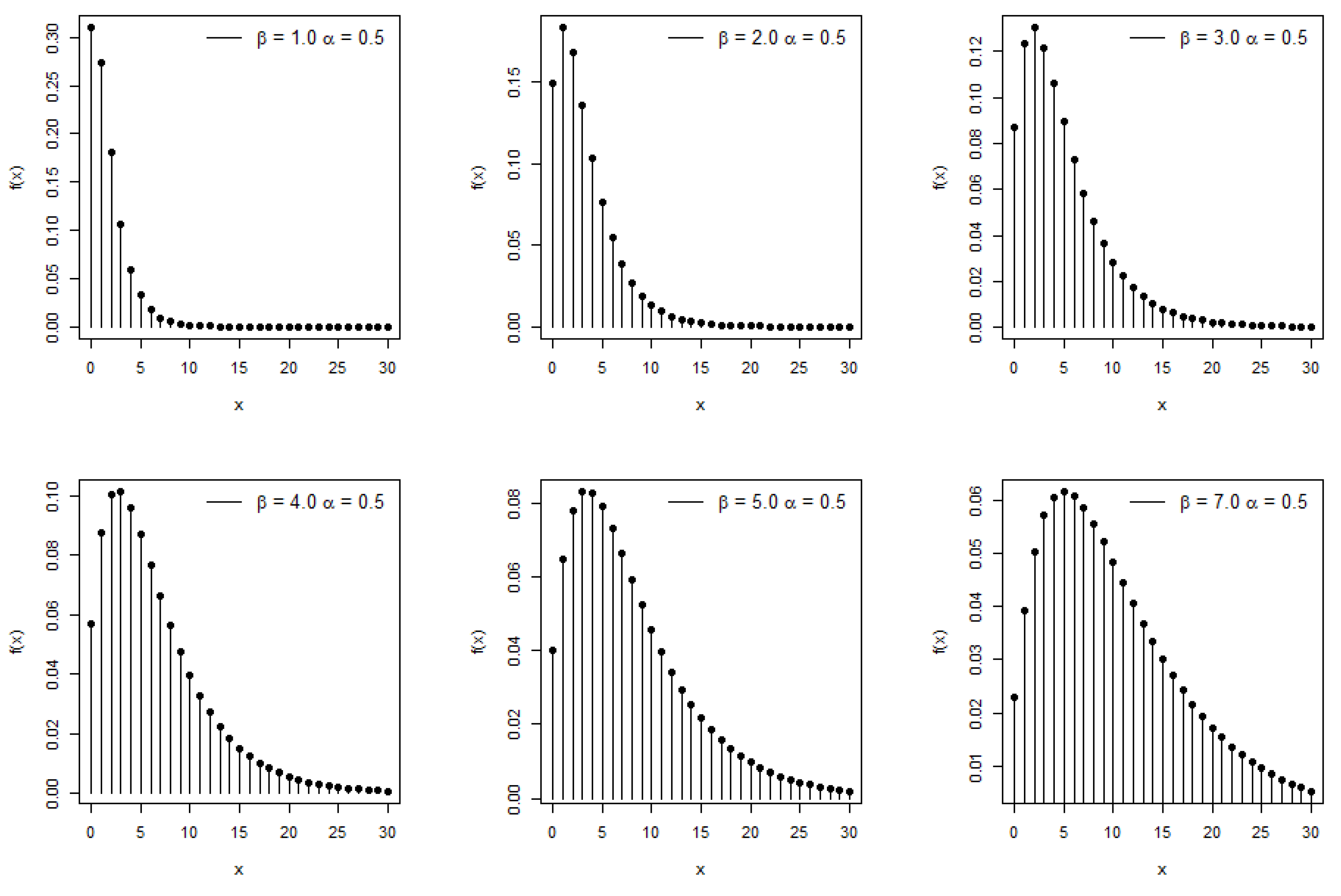
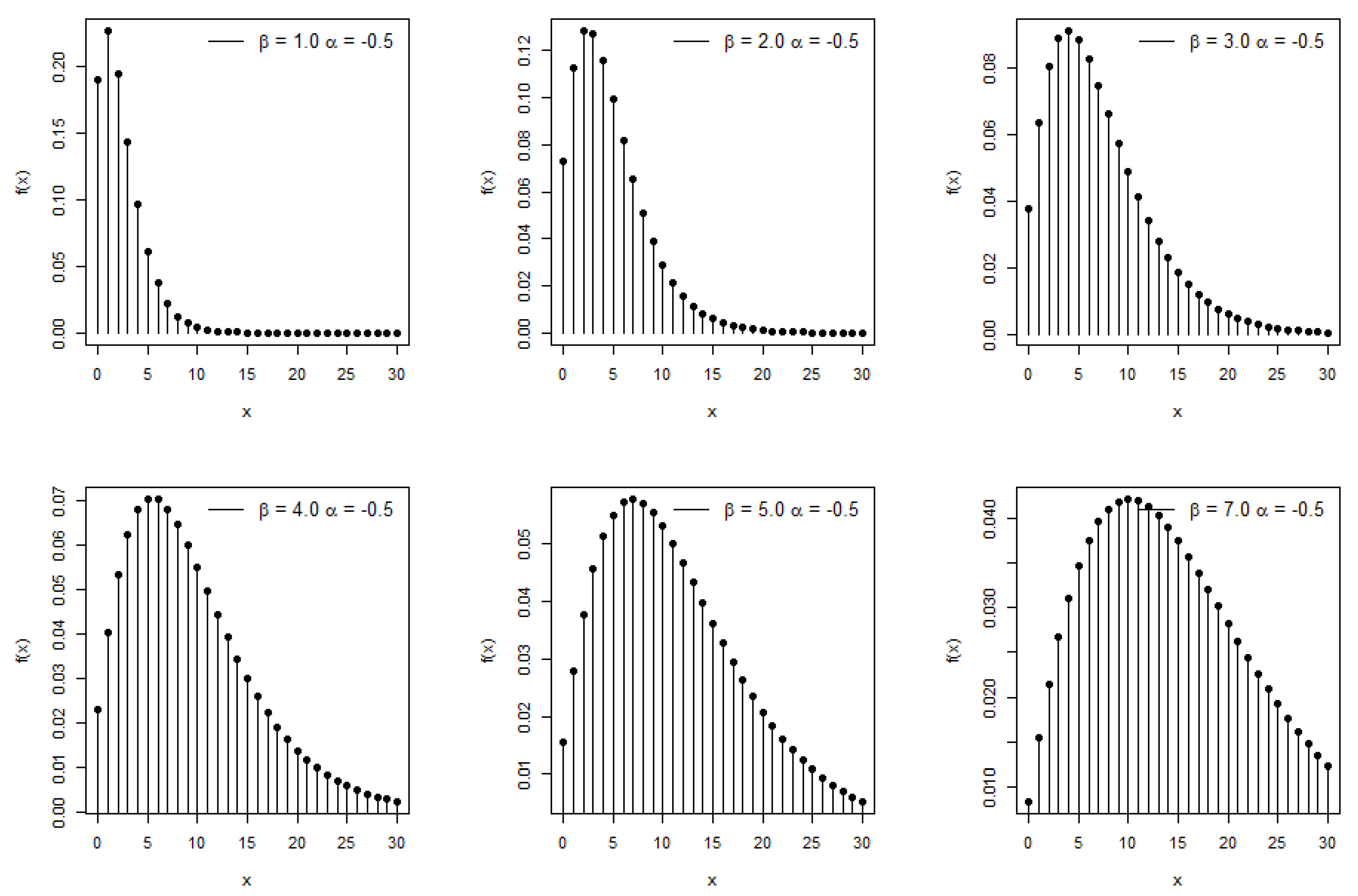
2. Derivation of New Model

Let a random variable, $X$, follow a transmuted moment exponential distribution, i.e., $X~TMEx\left(\beta ,\alpha \right)$. Then, its probability density function (PDF) is given by

$$f\left(x;\beta \right)=\left(1-\alpha +2\alpha \left(1+\frac{x}{\beta }\right)\exp \left(-\frac{x}{\beta }\right)\right)\frac{x}{{\beta }^2}\exp \left(-\frac{x}{\beta }\right).$$

(1)

If a random variable, $X$, has the stochastic form shown below, it is said to follow the Poisson transmuted moment exponential distribution:

$$\begin{gathered} \left(X|\lambda \right)~P_0\left(\lambda \right) \\ \left(\lambda |\beta ,\alpha \right)~TMEx\left(\beta ,\alpha \right) \end{gathered}$$

$\lambda >0,\beta >0,$ and $0<\alpha <1$. The unconditional distribution of $X$ is known as the Poisson transmuted moment exponential distribution and is denoted by $PTMEx\left(\beta ,\alpha \right)$. Its probability mass function (pmf) is calculated as follows:

$$\begin{array}{c}P\left(X=x\right)={\int }_0^{\infty }P\left(X=\frac{x}{\lambda }\right)f_{\mathsf{\Lambda }}\left(\lambda ;\beta ,\alpha \right)d\lambda ,\hfill \\ \hspace{1em}\hspace{1em}\hspace{1em} ={\int }_0^{\infty }\frac{e^{-\lambda }{\lambda }^x}{x!}\left(1-\alpha +2\alpha \left(1+\frac{\lambda }{\beta }\right)\exp \left(-\frac{\lambda }{\beta }\right)\right)\frac{\lambda }{{\beta }^2}\exp \left(-\frac{\lambda }{\beta }\right)d\lambda ,\hfill \\ \hspace{1em}\hspace{1em}\hspace{1em}\hspace{1em}=\left(1+x\right)\left(\frac{\left(1-\alpha \right){\left(1+\frac{1}{\beta }\right)}^{-x}}{{\left(1+\beta \right)}^2}+\frac{2\alpha {\left(\frac{2+\beta }{\beta }\right)}^{-x}\left(4+x+\beta \right)}{{\left(2+\beta \right)}^3}\right),\hfill \\ \hspace{1em}\hspace{1em}\hspace{1em}\hspace{1em}={\beta }^x\left(1+x\right)\left(\frac{\left(1-\alpha \right)}{{\left(1+\beta \right)}^{2+x}}+\frac{2\alpha \left(4+x+\beta \right)}{{\left(2+\beta \right)}^{3+x}}\right).\hfill \end{array}$$

(2)

Plots of the pmf for the PTMEx distribution for different parameter selections are displayed in Figure 1, which may be found below. The behavior of the pmf demonstrates that the probabilities can take on a declining form and be unimodal. The parameter values determine the geometry of the pmf, which may or may not be symmetrical.

Further, the cumulative distribution function (cdf) of the PTMEx distribution is

$$\begin{gathered} \hspace{1em}\hspace{1em}\hspace{1em}\hspace{1em}\hspace{1em}\hspace{1em}\hspace{1em}\hspace{1em}\hspace{1em}\hspace{1em}\hspace{1em}F\left(x\right)=\frac{{\beta }^{2x}}{{\left(1+\beta \right)}^{2+x}{\left(2+\beta \right)}^{3+x}}\left({\left(2+\beta \right)}^3\left({\left(1+\beta \right)}^2{\left(\frac{\left(1+\beta \right)\left(2+\beta \right)}{{\beta }^2}\right)}^x-\beta {\left(\frac{2+\beta }{\beta }\right)}^x\left(2+x+\beta \right)\right) \\ +\alpha \beta \left({\left(2+\beta \right)}^3{\left(\frac{2+\beta }{\beta }\right)}^x\left(2+x+\beta \right) \\ \hspace{1em}\hspace{1em}\hspace{1em}\hspace{1em}\hspace{1em}\hspace{1em}\hspace{1em}\hspace{1em}-{\left(1+\frac{1}{\beta }\right)}^x{\left(1+\beta \right)}^2\left(10+x^2+\beta \left(6+\beta \right)+x\left(7+2\beta \right)\right)\right)\right). \end{gathered}$$

(3)

Moments and Associated Measures

In this subsection, some moment metrics are used to study some aspects of the PTMEx distribution.

The moment-generating function can be derived as

$$\begin{array}{c}{M}_X\left(t\right)=E\left(e^{tX}\right),\hfill \\ \hspace{1em}\hspace{1em} ={\displaystyle \sum _{x=0}^{\infty }}{e}^{tx}\left\{\left(1+x\right)\left(\frac{\left(1-\alpha \right){\left(1+\frac{1}{\beta }\right)}^{-x}}{{\left(1+\beta \right)}^2}+\frac{2\alpha {\left(\frac{2+\beta }{\beta }\right)}^{-x}\left(4+x+\beta \right)}{{\left(2+\beta \right)}^3}\right)\right\},\hfill \\ \hspace{1em}\hspace{1em} =\frac{1-\alpha }{{\left(1+\beta -e^t\beta \right)}^2}+\frac{2\alpha }{{\left(2+\beta -e^t\beta \right)}^2}-\frac{4\alpha }{{\left(-2+\left(-1+e^t\right)\beta \right)}^3}.\hfill \end{array}$$

(4)

The first four moments of X can be derived as

$$\begin{array}{c}E\left(X\right)=\frac{1}{4}\left(8\beta -3\alpha \beta \right),\hfill \\ E\left(X^2\right)=\frac{1}{4}\left(8\beta -3\alpha \beta +24{\beta }^2-15\alpha {\beta }^2\right),\hfill \\ E\left(X^3\right)=\frac{1}{4}\left(8\beta -3\alpha \beta +72{\beta }^2-45\alpha {\beta }^2+96{\beta }^3-75\alpha {\beta }^3\right),\hfill \end{array}$$

and

$$E\left(X^4\right)=\frac{1}{4}\left(8\beta -3\alpha \beta +168{\beta }^2-105\alpha {\beta }^2+576{\beta }^3-450\alpha {\beta }^3+480{\beta }^4-420\alpha {\beta }^4\right).$$

The variance (var), dispersion index (DI), and coefficient of variation (CV) of the PTMEx distribution are given by

$$\begin{array}{c}Var\left(X\right)=\frac{1}{16}\beta \left(32\left(1+\beta \right)-3\alpha \left(4+\left(4+3\alpha \right)\beta \right)\right),\hfill \\ DI\left(X\right)=\frac{\beta \left(32\left(1+\beta \right)-3\alpha \left(4+\left(4+3\alpha \right)\beta \right)\right)}{4(8\beta -3\alpha \beta )},\hfill \end{array}$$

and

$$\begin{array}{c}CV\left(X\right)=\frac{(8-3\alpha )\beta }{\sqrt{\beta \left(32\right(1+\beta )-3\alpha (4+(4+3\alpha )\beta \left)\right)}}.\hfill \end{array}$$

The third and fourth moments about the mean are

$$\begin{array}{c}{\mu }_3=\frac{1}{32}\beta \left(-27{\alpha }^3{\beta }^2-54{\alpha }^2\beta \left(1+\beta \right)+64\left(1+\beta \right)\left(1+2\beta \right)-24\alpha \left(1+\beta \left(3+\beta \right)\right)\right),\hfill \\ {\mu }_4=\frac{1}{256}\beta (-243{\alpha }^4{\beta }^3-648{\alpha }^3{\beta }^2\left(1+\beta \right)-576{\alpha }^2\beta \left(1+6\beta +4{\beta }^2\right)+512\left(1+\beta \right)\left(1+12\beta \left(1+\beta \right)\right)\hfill \\ \hspace{1em}\hspace{1em}\hspace{1em}\hspace{1em}\hspace{1em} -192\alpha \left(1+\beta \right)\left(1+6\beta \left(3+2\beta \right)\right)).\hfill \end{array}$$

Then, the coefficients of skewness and kurtosis are given by

$$\begin{array}{c}\mathrm{C}\mathrm{S}=\frac{{\mu }_3}{{\left({\mu }_2\right)}^{\frac{3}{2}}}\hfill \\ \mathrm{C}\mathrm{S}=\frac{2\beta \left(-27{\alpha }^3{\beta }^2-54{\alpha }^2\beta \left(1+\beta \right)+64\left(1+\beta \right)\left(1+2\beta \right)-24\alpha \left(1+\beta \left(3+\beta \right)\right)\right)}{{\left(\beta \left(32\left(1+\beta \right)-3\alpha \left(4+\left(4+3\alpha \right)\beta \right)\right)\right)}^{3/2}},\hfill \end{array}$$

and

$$\begin{array}{c}\mathrm{C}\mathrm{K}=\frac{{\mu }_4}{{\left({\mu }_2\right)}^2}\hfill \\ \hspace{1em}\hspace{1em}\mathrm{C}\mathrm{K}=-\frac{243{\alpha }^4{\beta }^3+648{\alpha }^3{\beta }^2\left(1+\beta \right)+576{\alpha }^2\beta \left(1+6\beta +4{\beta }^2\right)-512\left(1+\beta \right)\left(1+12\beta \left(1+\beta \right)\right)+192\alpha \left(1+\beta \right)\left(1+6\beta \left(3+2\beta \right)\right)}{\beta {\left(32\left(1+\beta \right)-3\alpha \left(4+\left(4+3\alpha \right)\beta \right)\right)}^2}.\hfill \end{array}$$

Table 1. Values of some computational statistics for PTMEx distribution.

Parameters		Measures
$\mathit{\beta }$	$\mathit{\alpha }$	Mean	Variance	Skewness	Kurtosis	CV	DI
0.5	−0.8	1.3000	1.8600	1.3695	5.5696	1.0491	1.4308
	−0.5	1.1875	1.7461	1.4609	5.9067	1.1128	1.4704
	−0.2	1.0750	1.6069	1.5621	6.3336	1.1792	1.4948
	0.0	1.0000	1.5000	1.6330	6.6667	1.2247	1.5000
	0.2	0.9250	1.3819	1.7037	7.0283	1.2708	1.4939
	0.5	0.8125	1.1836	1.7963	7.5506	1.3390	1.4567
	0.8	0.7000	0.9600	1.8244	7.6852	1.3997	1.3714
1.0	−0.8	2.6000	4.8400	1.2464	5.2747	0.8462	1.8615
	−0.5	2.3750	4.6094	1.3275	5.5368	0.9040	1.9408
	−0.2	2.1500	4.2775	1.4267	5.9217	0.9620	1.9895
	0.0	2.0000	4.0000	1.5000	6.2500	1.0000	2.0000
	0.2	1.8500	3.6775	1.5751	6.6303	1.0366	1.9878
	0.5	1.6250	3.1094	1.6735	7.2268	1.0851	1.9135
	0.8	1.4000	2.4400	1.6813	7.3870	1.1157	1.7429
1.5	−0.8	3.9000	8.9400	1.2105	5.2069	0.7667	2.2923
	−0.5	3.5625	8.5898	1.2847	5.4302	0.8227	2.4112
	−0.2	3.2250	8.0119	1.3840	5.7992	0.8777	2.4843
	0.0	3.0000	7.5000	1.4606	6.1333	0.9129	2.5000
	0.2	2.7750	6.8869	1.5412	6.5368	0.9457	2.4818
	0.5	2.4375	5.7773	1.6499	7.2096	0.9861	2.3702
	0.8	2.1000	4.4400	1.6559	7.4460	1.0034	2.1143

provides some numerical values for the PTMEx distribution’s mean, variance, DI, skewness, and kurtosis for various parameter choices. The PTMEx model, with regard to its mean and variance, is a decreasing function of $\alpha$, while it increases when its $\beta$ parameter increases. The PTMEx distribution is overdispersed and asymmetrically right-skewed.

3. Parameter Estimation

In this section, the parameters of the proposed distribution are estimated using maximum likelihood and Bayesian estimation techniques. Further, a comprehensive simulation study is utilized to identify efficient estimation methods for the PTMEx distribution.

3.1. Maximum Likelihood Estimation

Let $X_1,X_2,\dots ,X_n$ be a random sample of size $n$ from the PTMEx distribution and $x_1,x_2,\dots ,x_n$ be the observations of $X_1,X_2,\dots ,X_n$. The log-likelihood function is

$$l\left(\alpha ,\beta \right)=\sum _{i=1}^n{x}_i\log \left(\beta \right)+\sum _{i=1}^n{(1+x}_i)+\sum _{i=1}^n\log \left\{\frac{\left(1-\alpha \right)}{{\left(1+\beta \right)}^{2+x_i}}+\frac{2\alpha \left(4+x+\beta \right)}{{\left(2+\beta \right)}^{3+x_i}}\right\}.$$

(5)

The maximum likelihood estimates (MLEs) can be derived from Equation (5) by differentiating for parameters. Now, by solving $\frac{\partial l\left(\alpha ,\beta \right)}{\partial \alpha }=0$ and $\frac{\partial l\left(\alpha ,\beta \right)}{\partial \beta }=0$, we obtain the following non-linear equations:

$$\sum _{i=1}^n\frac{2{\left(2+\beta \right)}^{-3-x_i}\left(4+x_i+\beta \right)-{\left(1+\beta \right)}^{-2-x_i}}{(1-\alpha ){\left(1+\beta \right)}^{-2-x_i}+2\alpha {\left(2+\beta \right)}^{-3-x_i}\left(4+x_i+\beta \right)}=0,$$

(6)

and

$$\sum _{i=1}^n\frac{x_i}{\beta }+\sum _{i=1}^n\frac{\left(2+x_i\right)\left(\left(\alpha -1\right){\left(1+\beta \right)}^{-3-x_i}-2\alpha {\left(2+\beta \right)}^{-4-x_i}\left(5+x+\beta \right)\right)}{(1-\alpha ){(1+\beta )}^{-2-x_i}+2\alpha {(2+\beta )}^{-3-x_i}(4+x+\beta )}=0.$$

(7)

The solution of Equations (6) and (7) gives the MLEs. As we can see, obtaining the exact solution to these equations is not possible, so we solve them using iterative procedures. For this purpose, we use the “optim” command using R software.

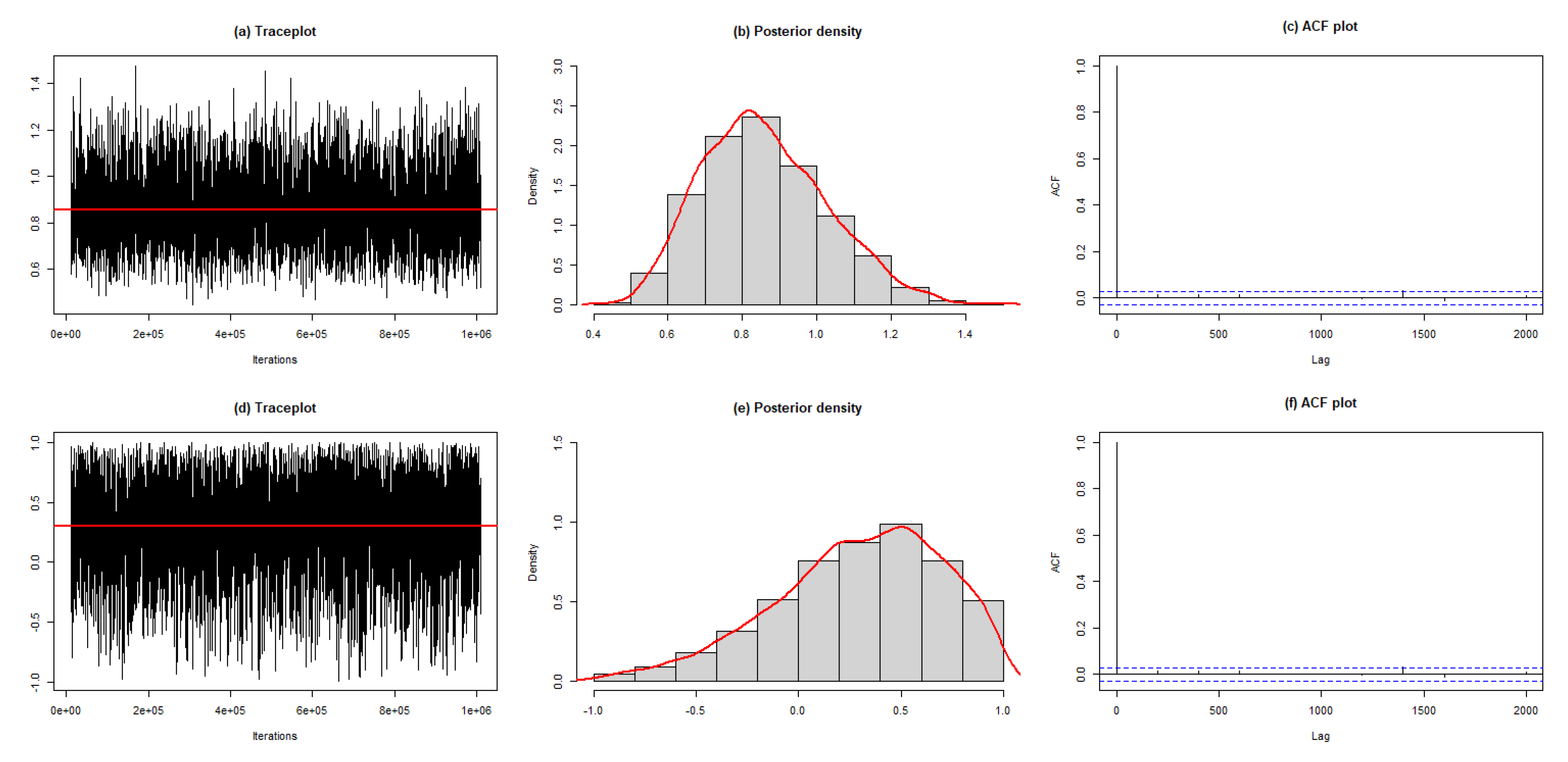
3.2. Bayesian Estimation

A Bayesian estimation procedure is also utilized to estimate the PTMEx distribution parameters. For a Bayesian estimation, it is essential to specify a prior distribution for each parameter of the PTMEx distribution. We can assume a gamma distribution for $\beta$ and a uniform distribution for the $\alpha$ parameter. The pdfs of the gamma and uniform distributions, with parameters, are as follows:

$$\beta ~Gamma\left(a,b\right),a,b>0,$$

(8)

and

$$\alpha ~Uniform\left(c,d\right),c,d>0$$

(9)

where $a$, $b$, $c,$ and $d$ are known as the hyperparameters.

The joint posterior density is given by

$$\psi \left(a,b,c,d|x\right)\propto L_n\times \psi \left(\beta \right)\times \psi \left(\alpha \right).$$

(10)

where $L_n$ is the likelihood function of the PTMEx distribution, $\psi \left(\beta \right)$ is the pdf of the gamma distribution, and $\psi \left(\alpha \right)$ is the pdf of the uniform distribution. Equation (10) makes it clear that there is no analytical way to obtain Bayesian estimates. As a result, we use the R (4.3.0) program to implement the Metropolis–Hastings algorithm of the Markov chain Monte Carlo (MCMC) methodology, a fantastic simulation tool.

For the Bayesian estimation, we generate 1,005,000 samples from the joint posterior distribution. To eliminate the effect of the initial values in the iterative procedure, we use a burn-in phase of 5000. A thinning interval of 200 is considered to have approximately independent samples. The Bayes parameter estimates are calculated as the means of samples chosen from the joint posterior distribution. Further, trace plots and the Geweke diagnostic are used to monitor the convergence of the simulated sequences.

Metropolis–Hastings (M-H) algorithm

Since the marginal posterior density lacks a closed form, Bayesian estimates cannot be obtained analytically. It is sampled using the Metropolis–Hastings (M-H) method. The M-H algorithm operates as follows:

• Start with the initial parameter values $\left({\alpha }^0,{\beta }^0\right)$.
• Set the iteration counter to $j=1$.
• Simulate the $\tilde{\alpha }$ and $\tilde{\beta }$ from the normal proposal distribution $N\left({\alpha }^{\left(j-1\right)},var\left({\alpha }^{\left(j-1\right)}\right)\right)$ and $N\left({\beta }^{\left(j-1\right)},var\left({\beta }^{\left(j-1\right)}\right)\right)$, respectively.
• Then, evaluate the acceptance probability:

$$\psi \left(\alpha \right)=\min \left[1,\frac{{\pi }^{*}\left(\tilde{\alpha }|{\beta }^{\left(j-1\right)}\right)}{{\pi }^{*}\left({\alpha }^{\left(j-1\right)}|{\beta }^{\left(j-1\right)}\right)}\right] \mathrm{a}\mathrm{n}\mathrm{d} \psi \left(\beta \right)=\min \left[1,\frac{{\pi }^{*}\left(\tilde{\beta }|{\beta }^{\left(j-1\right)}\right)}{{\pi }^{*}\left({\beta }^{\left(j-1\right)}|{\alpha }^{\left(j-1\right)}\right)}\right]$$

(11)

5

Then, generate $u_1$ and $u_2$ from the uniform distribution $Uniform\left(0,1\right)$.

6

If $u_1<\psi \left(\alpha \right)$, we consider ${\alpha }^{\left(j\right)}={\alpha }^{*}$; otherwise, set ${\alpha }^{\left(j\right)}={\alpha }^{\left(j-1\right)}$.

7

If $u_2<\psi \left(\beta \right)$, we consider ${\beta }^{\left(j\right)}={\beta }^{*}$; otherwise, set ${\beta }^{\left(j\right)}={\beta }^{\left(j-1\right)}$.

8

Change the counter from $j$ to $j+1$.

9

To obtain an accurate approximation for the estimates, we must repeat the procedures from (3)–(8). $N=10000$ repetitions to obtain values for the parameters, and this sample can be stated as follows: $\left({\alpha }^{\left(1\right)},{\beta }^{\left(1\right)}\right),\dots ,\left({\alpha }^{\left(N\right)},{\beta }^{\left(N\right)}\right)$.

4. Simulation

In this section, we conduct a comprehensive Monte Carlo simulation study to evaluate the performances of derived estimators. The absolute average estimates (AEs), mean relative errors (MREs), and mean square errors (MSEs) of five estimators are calculated in a simulation study with 10,000 iterations for sample sizes of n = 20, 50, 100, and 200. The following parameter settings are considered: $\mathrm{s}\mathrm{e}\mathrm{t} \mathrm{I}:\left(\beta =0.5;\alpha =-0.8\right)$, $\mathrm{s}\mathrm{e}\mathrm{t} \mathrm{I}\mathrm{I}:\left(\beta =0.5;\alpha =-0.5\right)$, $\mathrm{s}\mathrm{e}\mathrm{t} \mathrm{I}\mathrm{I}\mathrm{I}:\left(\beta =0.5;\alpha =-0.2\right)$, $\mathrm{s}\mathrm{e}\mathrm{t} \mathrm{I}\mathrm{V}:\left(\beta =0.5;\alpha =0.5\right),\mathrm{s}\mathrm{e}\mathrm{t} \mathrm{V}:\left(\beta =1.5;\alpha =0.5\right),$ and $\mathrm{s}\mathrm{e}\mathrm{t} \mathrm{V}\mathrm{I}:\left(\beta =1.5;\alpha =-0.5\right)$. All simulations generate samples from the PTMEx distribution.

Table 2. Parameter estimates, MSEs, and MREs of θ based on the maximum likelihood method.

Parameter	$\mathit{n}$	AE		MRE		MSE
		$\widehat{\mathit{\beta }}$	$\widehat{\mathit{\alpha }}$	$\widehat{\mathit{\beta }}$	$\widehat{\mathit{\alpha }}$	$\widehat{\mathit{\beta }}$	$\widehat{\mathit{\alpha }}$
$\beta =0.5$ $\alpha =-0.8$	50	0.5542	−0.5740	0.1083	−0.2825	0.0233	0.3661
	100	0.5448	−0.6135	0.0896	−0.2332	0.0175	0.2813
	200	0.5252	−0.6892	0.0504	−0.1385	0.0084	0.1649
	500	0.5129	−0.7327	0.0259	−0.0841	0.0038	0.0923
	1000	0.5025	−0.7884	0.0049	−0.0145	0.0012	0.0395
$\beta =0.5$ $\alpha =-0.5$	50	0.5262	−0.4536	0.0524	−0.0928	0.0209	0.3593
	100	0.5415	−0.3757	0.0830	−0.2486	0.0198	0.3749
	200	0.5284	−0.4502	0.0567	−0.0996	0.0135	0.2745
	500	0.5222	−0.4367	0.0444	−0.1266	0.0096	0.2053
	1000	0.5058	−0.4864	0.0117	−0.0273	0.0031	0.0846
$\beta =0.5$ $\alpha =-0.2$	50	0.4960	−0.3877	0.0079	−0.9385	0.0199	0.4136
	100	0.5086	−0.2877	0.0172	−0.4385	0.0156	0.3724
	200	0.5186	−0.2150	0.0371	−0.0751	0.0139	0.3089
	500	0.5213	−0.1594	0.0425	−0.2032	0.0096	0.2134
	1000	0.5159	−0.1697	0.0317	−0.1514	0.0066	0.1415
$\beta =0.5$ $\alpha =0.5$	50	0.5262	−0.4536	0.0524	−0.0928	0.0209	0.3593
	100	0.5415	−0.3757	0.083	−0.2486	0.0198	0.3749
	200	0.5284	−0.4502	0.0567	−0.0996	0.0135	0.2745
	500	0.5222	−0.4367	0.0444	−0.1266	0.0096	0.2053
	1000	0.5058	−0.4864	0.0117	−0.0273	0.0031	0.0846
$\beta =1.5$ $\alpha =0.5$	50	1.5044	0.4211	0.0029	0.1578	0.0998	0.2871
	100	1.4681	0.3977	0.0213	0.2046	0.0831	0.2145
	200	1.4856	0.4152	0.0096	0.1695	0.0675	0.1776
	500	1.4949	0.4434	0.0034	0.1133	0.0509	0.1112
	1000	1.5066	0.4720	0.0044	0.0560	0.0383	0.0841
$\beta =1.5$ $\alpha =-0.5$	50	1.5703	−0.4694	0.0469	−0.0611	0.1397	0.2699
	100	1.5543	−0.4627	0.0362	−0.0747	0.0826	0.1893
	200	1.5438	−0.4605	0.0292	−0.0790	0.0633	0.1381
	500	1.5131	−0.4930	0.0088	−0.0140	0.0265	0.0659
	1000	1.5019	−0.5030	0.0013	−0.0060	0.0064	0.0209

provides the AEs, MREs, and MSEs of the estimators. The results show that the MREs and MSEs for the combination of parameters tend toward zero as the sample size increases.

5. PTMEx Regression Model

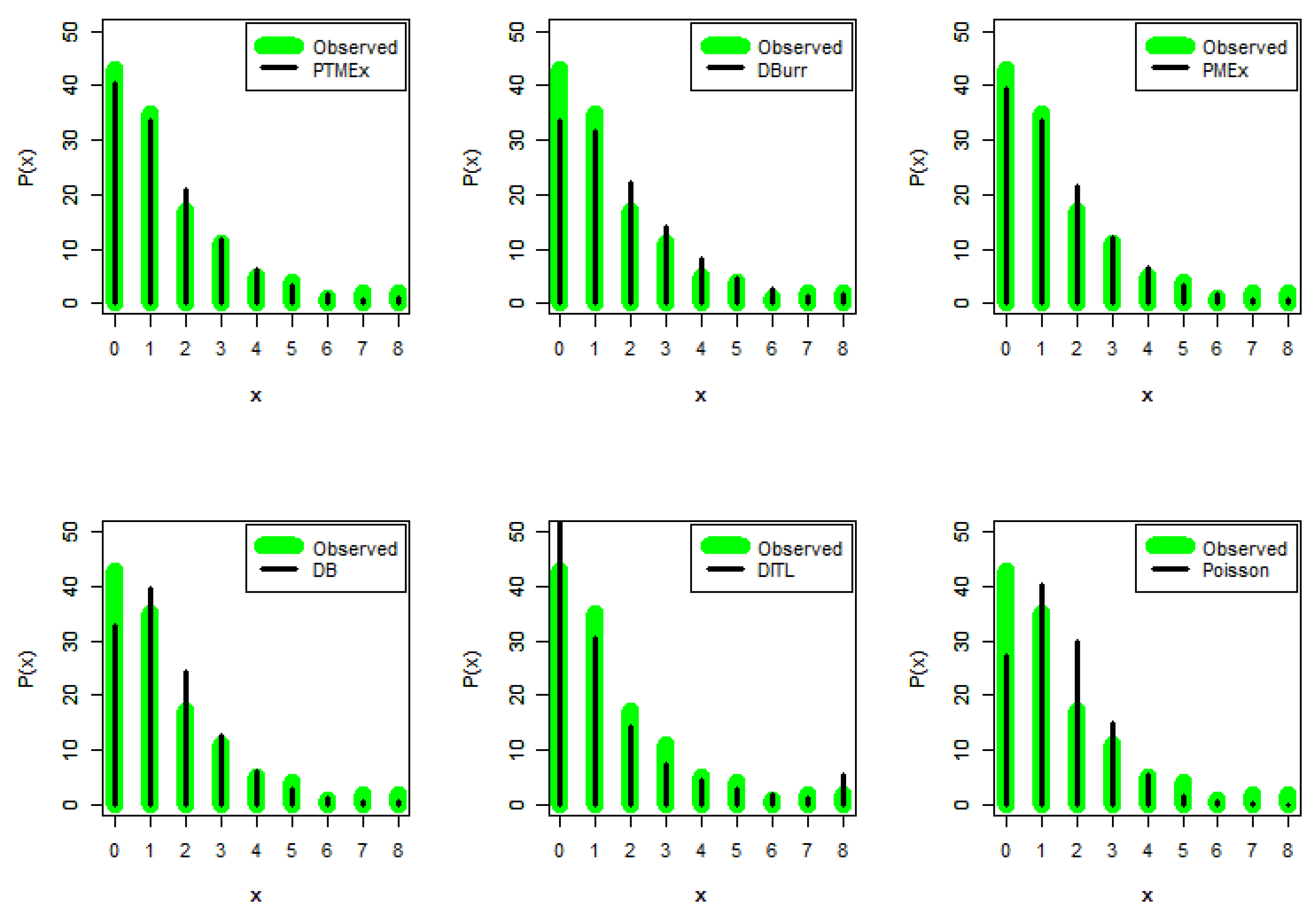
As was stated previously, the PTMEx distribution is regarded as having an excessively high degree of dispersion because the value of its dispersion parameter is greater than one. When dealing with datasets that have an excessive level of dispersion, the Poisson (P), negative binomial (NB), and Poisson quasi-Lindley (PQL) distributions can be replaced by the PTMEx distribution. This is due to the fact that the PTMEx distribution satisfies all three of these distributions’ criteria. In the following section of this paper, a new count regression model that is based on the PTMEx distribution is described. Let $\beta =4\mu /\left(8-3\alpha \right)$. Then, the pdf of the PTMEx distribution is given by

$$p\left(y_i;\alpha ,{\mu }_i\right)={\left(4{\mu }_i/\left(8-3\alpha \right)\right)}^{y_i}\times \left(1+y_i\right)\times \left(\frac{\left(1-\alpha \right)}{{\left(1+\left(4{\mu }_i/\left(8-3\alpha \right)\right)\right)}^{2+y_i}}+\frac{2\alpha \left(4+y_i+\left(4{\mu }_i/\left(8-3\alpha \right)\right)\right)}{{\left(2+\left(4{\mu }_i/\left(8-3\alpha \right)\right)\right)}^{3+y_i}}\right),$$

(12)

where $\mu >0,\alpha >0$, and $E\left(Y_i|\alpha ,{\mu }_i\right)={\mu }_i$.

We assume that the relationship between the response variable and the explanatory variables is in log-linear form, i.e.,

$${\mu }_i=\exp \left(\eta x_i^T\right),i=\mathrm{1,2},\dots ,n,$$

(13)

where $x_i^T=\left(x_{i1},x_{i2},\dots ,x_{ip}\right)$ is the vector of the covariates and $\eta ={\left({\eta }_0,{\eta }_1,{\eta }_2,\dots ,{\eta }_p\right)}^T$ is the unknown vector of the regression coefficients. Substituting Equation (13) into Equation (12), the pmf of $\left(Y_i|x_i^T\right)~PTMEx\left(\alpha ,{\mu }_i\right)$ is defined as a linear model form.

$$\begin{gathered} p\left(y_i;\alpha ,{\mu }_i\right)={\left(4\exp \left(\eta x_i^T\right)/\left(8-3\alpha \right)\right)}^{y_i}\times \left(1+y_i\right) \\ \hspace{1em}\hspace{1em}\hspace{1em}\hspace{1em} \times \left(\frac{\left(1-\alpha \right)}{{\left(1+\left(4\exp \left(\eta x_i^T\right)/\left(8-3\alpha \right)\right)\right)}^{2+y_i}} \\ \hspace{1em}\hspace{1em}\hspace{1em}\hspace{1em}\hspace{1em}\hspace{1em}+\frac{2\alpha \left(4+y_i+\left(4\exp \left(\eta x_i^T\right)/\left(8-3\alpha \right)\right)\right)}{{\left(2+\left(4\exp \left(\eta x_i^T\right)/\left(8-3\alpha \right)\right)\right)}^{3+y_i}}\right), \end{gathered}$$

(14)

The unknown model parameters can be estimated using the MLE method.

6. Empirical Study

In this section, two datasets are analyzed to prove the usefulness of the PTMEx distribution compared with the Poisson (Poi), Poisson moment exponential (PMEx) [19], discrete Burr (DBurr) [2], discrete Bilal (DB) [23], and discrete inverted Topp–Leone (DITL) [3] distributions. The maximum likelihood estimates (MLEs) are provided with adequacy measures such as the negative maximum log-likelihood $\left(-l\right)$, AIC, BIC, goodness-of-fit statistic $\left({\chi }^2\right)$, respective degrees of freedom (df), and p-values. Using the second and third datasets, the efficiency of the PTMEx regression model is examined by comparing the model with the Poisson (P), negative binomial (NB), Poisson generalized Lindley (PGL) [24], and Poisson transmuted record type exponential (PTRTE) [21] regression models.

6.1. European Corn Borer Data

The first dataset, with 120 observations, is associated with a biological experiment on a European corn borer [25], and the observations are presented in

Table 3. The MLEs and goodness-of-fit measures of all fitted models for the first dataset.

Count	Observed	Expected
		PTMEx	DBurr	PMEx	DB	DITL	Poisson
0	43	40.417	33.438	39.558	32.741	52.189	27.226
1	35	33.658	31.574	33.691	39.589	30.424	40.385
2	17	21.052	22.360	21.521	24.275	14.112	29.951
3	11	11.818	14.076	12.220	12.505	7.4663	14.809
4	5	6.3101	8.3071	6.5047	5.9678	4.3900	5.4915
5	4	3.2874	4.7064	3.3240	2.7359	2.7906	1.6291
6	1	1.6923	2.5924	1.6514	1.2256	1.8811	0.4027
7	2	0.8660	1.3988	0.8037	0.5414	1.3271	0.0853
8	2	0.8978	1.5473	0.7259	0.4193	5.4195	0.0188
Total	$n=120$	120	120	120	120	120	120
MLE	$\widehat{\beta }$	0.89444	0.51916	0.74161	2.3767	1.9840	1.4833
	$\widehat{\alpha }$	0.46514	2.35785	-	-	-	-
GOF Measures	$-l$	200.82	204.29	201.22	204.68	205.15	219.19
	AIC	405.64	412.59	404.44	411.35	412.30	440.38
	BIC	411.22	418.16	407.23	414.14	415.09	443.16
	${\chi }^2$	2.0825	6.5310	2.7268	9.6431	6.9771	21.761
	df	3.0	3.0	4.0	4.0	4.0	3.0
	p-value	0.72058	0.08845	0.60450	0.04689	0.13710	<0.0001

. The experiment was performed randomly on 8 hills in 15 replications, and the examiner counted the number of borers per hill of corn. The estimates, along with the comparison measures of the PTMEx distribution and the other competitive distributions, are listed in Table 3. The estimated pmfs of the fitted models over the observed data are presented in Figure 2. From Table 3 and Figure 2, we can infer that the PTMEx distribution yields a better fit compared to the other distributions.

The next step is to estimate the parameters of the PTMEx distribution using the previously given corn borer dataset using the Bayesian approach. The distributions of the posterior samples for both parameters are illustrated in Figure 3. The trace plots depict the development of the MCMC drawings across iterations, suggesting that the produced samples converge well. The autocorrelation function (ACF) plots reveal that the posterior samples are uncorrelated. The corresponding Geweke z-scores for $\beta$ and $\alpha$ are 0.2148 and 0.4915, also suggesting the satisfactory convergence of the samples to a stable distribution. The posterior means for $\beta$ and $\alpha$ are $\widehat{\beta }=0.8582$ (95% HDI: 0.5457 to 1.1705) and $\widehat{\alpha }=0.2974$ (95% HDI: −0.4441 to 0.9997). We can note that the ML and Bayesian estimates are fairly close to each other.

6.2. Length of Hospital Stay Data

The second dataset contains AZPRO data related to cardiovascular patients. This dataset comes from the COUNT package in R software. The observations were taken from Arizona cardiovascular patients’ files. The details of the variables are as follows:

• $y_i=$ length of patients’ stays at the hospital.
• $x_{1i}=$ cardiovascular procedure (1 = CABG, 0 = PTCA).
• $x_{2i}=$ gender (1 = male, 0 = female).
• $x_{3i}=$ admission type (1 = urgent, 0 = elective).
• $x_{4i}=$ age (1 = age > 75, 0 = age ≤ 75).

The systematic components of the regression models are defined by

$${\mu }_i=\exp \left({\eta }_0+{\eta }_1{x}_{1i}+{\eta }_2{x}_{2i}+{\eta }_3{x}_{3i}+{\eta }_4{x}_{4i}\right).$$

The mean and variance of the dependent variable are calculated as 8.8309 and 47.973, stating clear overdispersion.

Table 4. The findings of fitted count regression models of AZPRO data.

Para.	P		NB		PQL		PTMEx
	MLEs (SE)	p-Value	MLEs (SE)	p-Value	MLEs (SE)	p-Value	MLEs (SE)	p-Value
${\eta }_0$	1.4560 (0.0158)	<0.0001	1.0780 (0.0298)	<0.0001	1.3624 (0.0402)	<0.0001	1.3907 (0.0331)	<0.0001
${\eta }_1$	0.9603 (0.0122)	<0.0001	1.0866 (0.0243)	<0.0001	0.9746 (0.0317)	<0.0001	0.9877 (0.0260)	<0.0001
${\eta }_2$	−0.1239 (0.0118)	<0.0001	0.0724 (0.0249)	0.0030	−0.1273 (0.0332)	0.0001	−0.1275 (0.0272)	<0.0001
${\eta }_3$	0.3266 (0.0121)	<0.0001	0.5319 (0.0249)	<0.0001	0.3961 (0.0329)	<0.0001	0.3909 (0.0270)	<0.0001
${\eta }_4$	0.1222 (0.0124)	<0.0001	0.3161 (0.3161)	<0.0001	0.1180 (0.0353)	<0.0001	0.1224 (0.0289)	<0.0001
$\alpha$	-	-	-	-	0.8893 (0.0016)	-	0.9843 (0.0109)	-
$-l$	11,190		10,578		10,919		10,352
AIC	22,390		21,169		21,849		20,714
BIC	22,421		21,206		21,880		20,745

gives the parameter estimates and results of the information criteria.

Table 4 indicates that all parameter estimates are significant at the 5% level of significance because the p-values for all parameter estimates are less than 5%. Further, the table makes it abundantly evident that the PTMEx regression model has the highest log-likelihood value, and the model’s AIC also shows that it fits the data better than the other two models.

7. Conclusions

In the event that there is overdispersion, it is unavoidable to locate new counting models. These models will offer a greater number of opportunities to better fit the actual datasets by selecting the appropriate models in accordance with the circumstances. In light of this, a novel two-parameter overdispersed distribution known as the “Poisson transmuted moment exponential distribution” is presented and researched here. The explicit expressions of the moment-generating function, moments, and others are among the fundamental qualities that were derived. Other fundamental properties that were derived include the mean, variance, and kurtosis. Both a classical and a Bayesian approach were utilized in order to estimate the model parameters. We also developed a new regression model for count data that was based on the PTMEx distribution. We compared this model to previous regression models that were based on actual data. This development is substantially more important. The first real-world asymmetric dataset, consisting of biological experiment data, was used to highlight the usage of the new methodology. The second real-world asymmetric dataset, consisting of information on the length of hospital stays, was also used.

8. Future Work

In the future, there may be several potential areas of work related to the new two-parameter discrete distribution. Here are some possibilities:

Further investigation of distribution properties: Researchers may delve deeper into exploring the mathematical properties of the proposed distribution. This could involve deriving additional moments, investigating the shape of the probability mass function, or exploring relationships with other existing distributions.

• Estimation methods: Future work could focus on developing efficient and accurate estimation methods for the parameters of the proposed distribution. This could involve maximum likelihood estimation, Bayesian estimation, or robust estimation techniques. Researchers may also explore the properties of the estimators, such as their asymptotic behavior and efficiency.
• Regression modeling: The new discrete distribution could be incorporated into regression models to analyze its performance in predicting or explaining the relationships between variables. This could involve developing regression frameworks, such as generalized linear models or zero-inflated models, that utilize the proposed distribution as the response variable. Researchers could also explore model selection criteria and compare the performance of the new distribution with existing ones in regression settings.
• Simulation studies: Future research could involve conducting extensive simulation studies to evaluate the behavior of the proposed distribution under various scenarios. This could include examining its robustness to violations of assumptions, assessing the accuracy of parameter estimation methods, and comparing the performances of statistical tests based on the new distribution.
• Applications: Further exploration of practical applications could be an area of focus. Researchers may investigate real-world datasets with overdispersed and asymmetric characteristics to assess the adequacy of the proposed distribution in modeling such data. This could include applications in fields such as finance, epidemiology, ecology, or social sciences.
• Software development: To facilitate the adoption and usage of the new distribution, researchers may develop software packages or functions in statistical software platforms (e.g., R and Python) for estimating parameters, conducting inference, and implementing regression models based on the proposed distribution. This would make it easier for practitioners to apply the distribution in their own research or data analysis.

Overall, future work on the new two-parameter discrete distribution could involve a combination of theoretical investigations, methodological developments, empirical studies, and practical applications to establish its properties, estimation procedures, regression modeling capabilities, and usefulness in various fields.

References

1. Afify, A.Z.; Ahsan-ul-Haq, M.; Aljohani, H.M.; Alghamdi, A.S.; Babar, A.; Gómez, H.W. A new one-parameter discrete exponential distribution: Properties, inference, and applications to COVID-19 data. J. King Saud Univ.-Sci. 2022, 34, 102199. [Google Scholar] [CrossRef]
2. Ahsan-ul-Haq, M.; Al-bossly, A.; El-morshedy, M.; Eliwa, M.S. Poisson XLindley Distribution for Count Data: Statistical and Reliability Properties with Estimation Techniques and Inference. Comput. Intell. Neurosci. 2022, 2022, 6503670. [Google Scholar] [CrossRef] [PubMed]
3. Ahsan-ul-Haq, M.; Zafar, J. A new one-parameter discrete probability distribution with its neutrosophic extension: Mathematical properties and applications. Int. J. Data Sci. Anal. 2023, 1–11. [Google Scholar] [CrossRef]
4. Akdoğan, Y.; Kuş, C.; Asgharzadeh, A.; Kınacı, İ.; Sharafi, F. Uniform-geometric distribution. J. Stat. Comput. Simul. 2016, 86, 1754–1770. [Google Scholar] [CrossRef]
5. Al-Bossly, A.; Eliwa, M.S.; Ahsan-ul-Haq, M.; El-Morshedy, M. Discrete Logistic Exponential Distribution with Applications. Stat. Optim. Inf. Comput. 2023, 11, 629–639. [Google Scholar] [CrossRef]
6. Alghamdi, A.S.; Ahsan-ul-Haq, M.; Babar, A.; Aljohani, H.M.; Afify, A.Z. The discrete power-Ailamujia distribution: Properties, inference, and applications. AIMS Math. 2022, 7, 8344–8360. [Google Scholar] [CrossRef]
7. Aljohani, H.M.; Akdoğan, Y.; Cordeiro, G.M.; Afify, A.Z. The uniform Poisson–Ailamujia distribution: Actuarial measures and applications in biological science. Symmetry 2021, 13, 1258. [Google Scholar] [CrossRef]
8. Altun, E. A new one-parameter discrete distribution with associated regression and integer-valued autoregressive models. Math. Slovaca 2020, 70, 979–994. [Google Scholar] [CrossRef]
9. Altun, E. A new two-parameter discrete poisson-generalized Lindley distribution with properties and applications to healthcare data sets. Comput. Stat. 2021, 36, 2841–2861. [Google Scholar] [CrossRef]
10. Altun, E.; Cordeiro, G.M.; Ristić, M.M. An one-parameter compounding discrete distribution. J. Appl. Stat. 2021, 49, 1935–1956. [Google Scholar] [CrossRef]
11. Beall, G. The fit and significance of contagious distributions when applied to observations on larval insects. Ecology 1940, 21, 460–474. [Google Scholar] [CrossRef]
12. Coşkun, K.; AKdoğan, Y.; Asgharzadeh, A.; Kinaci, İ.; Karakaya, K. Binomial-discrete Lindley distribution. Commun. Fac. Sci. Univ. Ank. Ser. A1 Math. Stat. 2018, 68, 401–411. [Google Scholar]
13. Eldeeb, A.S.; Ahsan-ul-Haq, M.; Babar, A. A Discrete Analog of Inverted Topp-Leone Distribution: Properties, Estimation and Applications. Int. J. Anal. Appl. 2021, 19, 695–708. [Google Scholar]
14. Eldeeb, A.S.; Ahsan-ul-Haq, M.; Babar, A. A new discrete XLindley distribution: Theory, actuarial measures, inference, and applications. Int. J. Data Sci. Anal. 2023, 1–11. [Google Scholar] [CrossRef]
15. Eldeeb, A.S.; Ahsan-ul-Haq, M.; Eliwa, M.S. A discrete Ramos-Louzada distribution for asymmetric and over-dispersed data with leptokurtic-shaped: Properties and various estimation techniques with inference. AIMS Math. 2021, 7, 1726–1741. [Google Scholar] [CrossRef]
16. Erbayram, T.; Akdoğan, Y. A new discrete model generated from mixed Poisson transmuted record type exponential distribution. Ric. Mat. 2023, 1–23. [Google Scholar] [CrossRef]
17. Gómez-Déniz, E. A new discrete distribution: Properties and applications in medical care. J. Appl. Stat. 2013, 40, 2760–2770. [Google Scholar] [CrossRef]
18. Hosmer, D.W.; Lemeshow, S. Applied Logistic Regression; Wiley: Hoboken, NJ, USA, 2000. [Google Scholar]
19. Kempton, R.A. A generalized form of Fisher’s logarithmic series. Biometrika 1975, 62, 29–38. [Google Scholar] [CrossRef]
20. Krishna, H.; Pundir, P.S. Discrete Burr and discrete Pareto distributions. Stat. Methodol. 2009, 6, 177–188. [Google Scholar] [CrossRef]
21. Maya, R.; Huang, J.; Irshad, M.R.; Zhu, F. On Poisson Moment Exponential Distribution with Associated Regression and INAR(1) Process. Ann. Data Sci. 2023, 1–19. [Google Scholar] [CrossRef]
22. Nakagawa, T.; Osaki, S. The discrete Weibull distribution. IEEE Trans. Reliab. 1975, 24, 300–301. [Google Scholar] [CrossRef]
23. Sajjadnia, Z.; Sharafi, M.; Mamode Khan, N.; Soobhug, A.D. A new bivariate INAR(1) model with paired Poisson-weighted exponential distributed innovations. Commun. Stat. Simul. Comput. 2023, 1–19. [Google Scholar] [CrossRef]
24. Sankaran, M. The Discrete Poisson-Lindley Distribution. Biometrics 1970, 26, 145–149. [Google Scholar] [CrossRef]
25. Zeghdoudi, H.; Nedjar, S. On Poisson pseudo Lindley distribution: Properties and applications. J. Probab. Stat. Sci. 2017, 15, 19–28. [Google Scholar]
Figure 1. The pmf plots of the PTMEx distribution for some parametric values.
Symmetry 15 01289 g001aSymmetry 15 01289 g001b
Figure 2. Empirical pmfs of the fitted distributions for the corn borer dataset. We can see that the pmfs can be asymmetrically shaped.
Symmetry 15 01289 g002
Figure 3. Posterior samples for the model parameters of the PTMEx distribution.
Symmetry 15 01289 g003