Relaxation Functions Interpolating the Cole–Cole and Kohlrausch–Williams–Watts Dielectric Relaxation Models

Abstract

To describe non-Debye relaxation phenomena observed in dielectric materials, the Cole–Cole (CC) relaxation model in the frequency domain and the Kohlrausch–Williams–Watts (KWW) relaxation model in the time domain were introduced in the physics of dielectrics. In this paper, we propose a new relaxation model with two parameters besides a relaxation time by expressing the relaxation function in the time domain in terms of the Mittag–Leffler functions. The proposed model represents a group of non-Debye relaxation phenomena and shows a transition between the CC and the KWW models. The relaxation properties described by the new model are analyzed, including the response function, the normalized complex dielectric permittivity, dielectric storage and loss factors as well as the relaxation frequency and time spectral functions. The presented relaxation function has a concise form and is expected to be applied to more complex relaxation phenomena.

1. Introduction

Dielectric materials are extensively applied in the fields of science and engineering such as electromagnetics, microelectronics, materials, chemistry, biology, physics, etc., due to their ability to store and dissipate electromagnetic energy [1]. From a microcosmic viewpoint, the properties of dielectric materials are determined by the response mechanism of atoms and molecules to the applied electric field, which is commonly known as dielectric polarization [2]. Modeling the behavior and response of dielectric materials is important for theory and applications.

Consider a capacitor filled with a weakly conductive or polar dielectric medium and applied an external alternating voltage. In the alternating electric field, the dielectric permittivity ${\epsilon }^{*}$, the characteristic parameter of the dielectric medium, is complex and frequency dependent. The normalized complex dielectric permittivity has the form

$$\frac{{\epsilon }^{*}\left(\mathrm{i}\omega \right)-{\epsilon }_{\infty }}{{\epsilon }_0-{\epsilon }_{\infty }}=\widehat{\epsilon }\left(\mathrm{i}\omega \right)={\epsilon }^{\prime }\left(\omega \right)-\mathrm{i}{\epsilon }^{″}\left(\omega \right),$$

(1)

where ${\epsilon }_0$ and ${\epsilon }_{\infty }$ are the limiting low- and high-frequency dielectric permittivities of the given medium, and ${\epsilon }^{\prime }\left(\omega \right)$ and ${\epsilon }^{″}\left(\omega \right)$ are the real and negative imaginary parts of the normalized complex dielectric permittivity. ${\epsilon }^{\prime }\left(\omega \right)$ and ${\epsilon }^{″}\left(\omega \right)$ characterize the energy storage and loss in the medium, and are therefore called storage factor and loss factor, respectively, which are measurable through experiments.

The standard model in the physics of dielectrics is the Debye relaxation model with the form in the frequency domain

$$\widehat{\epsilon }\left(\mathrm{i}\omega \right)=\frac{1}{1+\mathrm{i}{\tau }_{*}\omega },$$

where ${\tau }_{*}$ is the relaxation time. The relaxation function in the time domain is the exponential function $\mathsf{\Psi }\left(t\right)=e^{-t/{\tau }_{*}}.$ However, non-exponential behavior was found in a large plethora of dielectric relaxation phenomena and different non-Debye empirical models were proposed [2,3,4,5,6,7].

The Cole–Cole (CC) relaxation model is a generalization of the Debye model in the frequency domain [3],

$$\widehat{\epsilon }\left(\mathrm{i}\omega \right)=\frac{1}{1+{\left(\mathrm{i}{\tau }_{*}\omega \right)}^{\alpha }},0<\alpha \le 1.$$

(2)

Recently, this model was used to derive a generalized skin depth formula of the polarized media in frequency-domain electromagnetic detection, and the method can be applied to the calculation of electromagnetic wave propagation depths in complex dispersive media [8]. In [9], the compatibility of composite materials was considered through a rheological analysis and Cole–Cole plot analysis. Other generalized relaxation models proposed in the frequency domain include the Davidson–Cole model [4], the Havriliak–Negami model [5], etc. [10]. A comprehensive introduction was presented in the review paper [7].

By the analysis of numerous experimental data in different dielectric materials, Jonscher [1,11] found that there exists a universal relaxation law following a fractional power law dependence for the asymptotic behaviors of low and high frequencies,

$$\begin{array}{ccc}\hfill {\epsilon }^{\prime }\left(0\right)-{\epsilon }^{\prime }\left(\omega \right)\sim {\omega }^m,& {\epsilon }^{″}\left(\omega \right)\sim {\omega }^m,& {\tau }_{*}\omega \ll 1,\hfill \end{array}$$

(3)

$$\begin{array}{ccc}\hfill {\epsilon }^{\prime }\left(\omega \right)\sim {\omega }^{n-1},& {\epsilon }^{″}\left(\omega \right)\sim {\omega }^{n-1},& {\tau }_{*}\omega \gg 1,\hfill \end{array}$$

(4)

where $0<m,n<1.$ Although this law was found in dielectric relaxations, the relaxation universality was also found in many other fields such as photoconductivity, chemical reaction kinetics, as well as mechanical relaxation [2].

Dielectric relaxation is associated with two causal functions (i.e., vanishing for $t<0$) in the time domain: the response function $\varphi \left(t\right)$ and the relaxation function $\mathsf{\Psi }\left(t\right)$, such that $\widehat{\epsilon }\left(\mathrm{i}\omega \right)$ is the pure imaginary Laplace transform (or the Fourier transform) of the response function $\varphi \left(t\right)$,

$$\widehat{\epsilon }\left(\mathrm{i}\omega \right)={\left.\mathcal{L}\left\{\varphi \right(t\left)\right\}\right|}_{s=\mathrm{i}\omega }=\tilde{\varphi }\left(\mathrm{i}\omega \right)={\mathsf{\int }}_0^{\infty }\varphi \left(t\right)e^{-\mathrm{i}\omega t}dt,$$

(5)

and the relaxation function $\mathsf{\Psi }\left(t\right)$ has the unitary initial value and its decaying rate represents the response function

$$\varphi \left(t\right)=-\frac{d\mathsf{\Psi }\left(t\right)}{dt},\mathsf{\Psi }\left(t\right)=1-{\mathsf{\int }}_0^t\varphi \left(t\right)dt.$$

(6)

From Equations (5) and (6), the relationship between the normalized complex dielectric permittivity and the relaxation function is revealed in the frequency domain

$$\widehat{\epsilon }\left(s\right)=1-s\tilde{\mathsf{\Psi }}\left(s\right),\mathrm{where}s=\mathrm{i}\omega .$$

(7)

Note that the Laplace transform is defined as $\mathcal{L}\left\{f\left(t\right)\right\}=\tilde{f}\left(s\right)={\int }_0^{\infty }f\left(t\right)e^{-st}dt$. The response function $\varphi \left(t\right)$ is the normalized depolarization current obtained when a steady electric field is removed from a sample. The relaxation function $\mathsf{\Psi }\left(t\right)$ describes the decay of polarization. In [10], the Jonscher indices of dielectric relaxation were proposed and determined from the experimental data of discharge current in barium stannate titanate. It is worth mentioning that the fractional kinetics provides a time domain model for non-Debye relaxation [7,12,13,14,15,16,17].

By Equation (7), the Laplace transform of the relaxation function of the CC model (2) is [12,18]

$${\tilde{\mathsf{\Psi }}}_{CC}\left(s\right)=\frac{{\tau }_{*}^{\alpha }{s}^{\alpha -1}}{1+{\tau }_{*}^{\alpha }{s}^{\alpha }}.$$

(8)

We note that, in [12], starting from the fractional Fokker–Planck equation, the corresponding relaxation function was derived in terms of the Mittag–Leffler function. In [19], the relaxation function was identified with the survival probability of a relaxing system described by a fractal time random walk model, and its frequency domain response takes exactly the CC pattern.

The Kohlrausch–Williams–Watts (KWW) relaxation model was introduced starting from its relaxation function in the time domain

$${\mathsf{\Psi }}_{KWW}\left(t\right)=exp\left(-{\left(\frac{t}{{\tau }_{*}}\right)}^{\alpha }\right),0<\alpha \le 1.$$

(9)

which is known as the stretched exponential function, and was first introduced by Kohlrausch in 1854 to describe the discharge relaxation phenomenon in Leiden jar capacitors [20,21]. Successively, this model was rediscovered by Williams and Watts [6] in 1970 to describe non-symmetric loss curves in anomalous dielectric relaxation. Other applications include viscoelastic shear oscillation [21], large-scale chain dynamics [21], recurrent time distribution of extreme events [22], etc. [23].

In this work, we present a new relaxation function with two parameters besides a relaxation time in terms of the Mittag–Leffler function, which joins the CC model in the frequency domain and the KWW model in time domain.

The Mittag–Leffler function with two parameters is defined by the series expansion [18,24]

$$E_{\alpha ,\rho }\left(z\right)=\sum _{k=0}^{\infty }\frac{z^k}{\mathsf{\Gamma }(\alpha k+\rho )},\alpha >0,\rho >0,z\in C,$$

(10)

where $\mathsf{\Gamma }(·)$ denotes the gamma function which is a generalization of the single parameter version $E_{\alpha }\left(z\right)=E_{\alpha ,1}\left(z\right).$ The Mittag–Leffler function satisfies the Laplace transform formula

$$\mathcal{L}\left\{z^{\rho -1}{E}_{\alpha ,\rho }(-b{z}^{\alpha })\right\}=\frac{s^{\alpha -\rho }}{s^{\alpha }+b},\alpha >0,\rho >0,b>0,\mathrm{Re}\left(s\right)>b^{1/\alpha }.$$

(11)

For a negative argument, the Mittag–Leffler function has the following asymptotic expansion

$$E_{\alpha ,\rho }(-z)\sim \sum _{k=1}^{\infty }\frac{{(-1)}^{k-1}}{\mathsf{\Gamma }(\rho -\alpha k)z^k},z\to +\infty ,0<\alpha \le 1,\rho >0.$$

(12)

In Section 2, we introduce a relaxation function with two parameters besides a relaxation time in terms of the Mittag–Leffler function, which interpolates the CC model in the frequency domain and the KWW model in the time domain. In Section 3, the response function and the complex dielectric permittivity are derived and analyzed. In Section 4, the relaxation frequency and time spectral functions are considered. Section 5 discusses the obtained results. Section 6 summarizes our conclusions.

2. Relaxation Functions Joining CC and KWW Models

By using Equations (8) and (11), the relaxation function of the CC model in Equation (2) is derived through the inverse Laplace transform as [12]

$${\mathsf{\Psi }}_{CC}\left(t\right)=E_{\alpha ,1}\left(-{\left(\frac{t}{{\tau }_{*}}\right)}^{\alpha }\right),0<\alpha \le 1.$$

(13)

In terms of the Mittag–Leffler function, the relaxation function of the KWW model in Equation (9) has the expression

$${\mathsf{\Psi }}_{KWW}\left(t\right)=E_{1,1}\left(-{\left(\frac{t}{{\tau }_{*}}\right)}^{\alpha }\right),0<\alpha \le 1.$$

(14)

Observing the two relaxation functions in Equations (13) and (14) motivates us to present an intermediate relaxation function by adding a parameter,

$$\mathsf{\Psi }\left(t\right)=\mathsf{\Psi }(t;\alpha ,\gamma )=E_{\alpha ,1}\left(-{\left(\frac{t}{{\tau }_{*}}\right)}^{\gamma }\right),0<\gamma \le \alpha \le 1,$$

(15)

where ${\tau }_{*}>0$ is the relaxation time. The model (15) becomes the CC model in (13) if $\alpha =\gamma$, and becomes the KWW model in (14) if $\alpha =1$. The case of $\alpha =\gamma =1$ reduces to the Debye relaxation. For the relaxation function and the latter response function, dielectric permittivity and spectral functions, whenever parameters need to be emphasized, they will be written out explicitly, such as for the special parameter values $\mathsf{\Psi }(t;\alpha ,\alpha )$ and ${\epsilon }^{\prime }(\omega ;1,\gamma )$. Note that the Mittag–Leffler function can be conveniently evaluated using Mathematica or Matlab [25,26,27]. All figures in this paper were generated using Mathematica 11.3.

First, we show the complete monotonicity of the relaxation function (15). Note that a function $f\left(x\right)$ is completely monotonic on the interval $0<x<+\infty$ if the following conditions are satisfied [24,28]

$${(-1)}^n{f}^{\left(n\right)}\left(x\right)\ge 0,x>0,n=0,1,2,\dots .$$

(16)

A Bernstein function $g\left(x\right)\ge 0$, $0<x<+\infty$ means that its derivative $g^{\prime }\left(x\right)$ is completely monotonic [29,30].

Proposition 1.

The relaxation function $\mathsf{\Psi }\left(t\right)$ in (15) and the corresponding response function $\varphi \left(t\right)$ are completely monotone.

Proof. 

The Mittag–Leffler function $E_{\alpha ,1}(-u)$ is complete monotone on the interval $0<u<+\infty$ [31], and the power function $u={\left(t/{\tau }_{*}\right)}^{\gamma }$ is a Bernstein function. The composition of a completely monotone function and a Bernstein function is another completely monotone function [29]. Thus, the relaxation function $\mathsf{\Psi }\left(t\right)$ in (15) is completely monotone. From the definition (6), the response function $\varphi \left(t\right)$ is also completely monotone. □

Complete monotonicity is essential for the physical acceptability and realization of the dielectric models [32]. Furthermore, complete monotonicity ensures the existence of non-negative spectral functions [29], which will be considered in Section 4.

Note that Oliveira et al. [15] derived a relaxation function starting from the fractional differential equation of Caputo type, known as the Kilbas and Saigo function (Equation (8) or (10) in [15]), which also includes as particular cases the CC model and KWW model, but is different from our model (15). Here, the relaxation function (15) is proven to be completely monotone, but such a conclusion is difficult to be proven for the relaxation function in [15]. We also mention that the conditions of complete monotonicity involving the Prabhakar function [33] (also known as the three-parameter Mittag–Leffler function) were investigated in [34,35,36] with the help of the closed form of the Laplace transform

$$\mathcal{L}\left\{t^{\beta -1}{E}_{\alpha ,\beta }^{\gamma }(-t^{\alpha })\right\}=\frac{s^{\alpha \gamma -\beta }}{{(s^{\alpha }+1)}^{\gamma }}.$$

(17)

From the definition formula (10) and the asymptotic expansion (12) of the Mittag–Leffler function, the asymptotic behaviors of the relaxation function for small and large arguments are

$$\mathsf{\Psi }(t;\alpha ,\gamma )\sim 1-\frac{1}{\mathsf{\Gamma }(1+\alpha )}{\left(\frac{t}{{\tau }_{*}}\right)}^{\gamma },t\to 0^{+},$$

(18)

and

$$\mathsf{\Psi }(t;\alpha ,\gamma )\sim \frac{1}{\mathsf{\Gamma }(1-\alpha )}{\left(\frac{t}{{\tau }_{*}}\right)}^{-\gamma },t\to +\infty ,$$

(19)

respectively. Notice that the right-hand side of Equation (19) vanishes if $\alpha =1$. The reason is that the KWW relaxation function decays in the stretched exponential function as $t\to +\infty$, more rapidly than any algebraic decay.

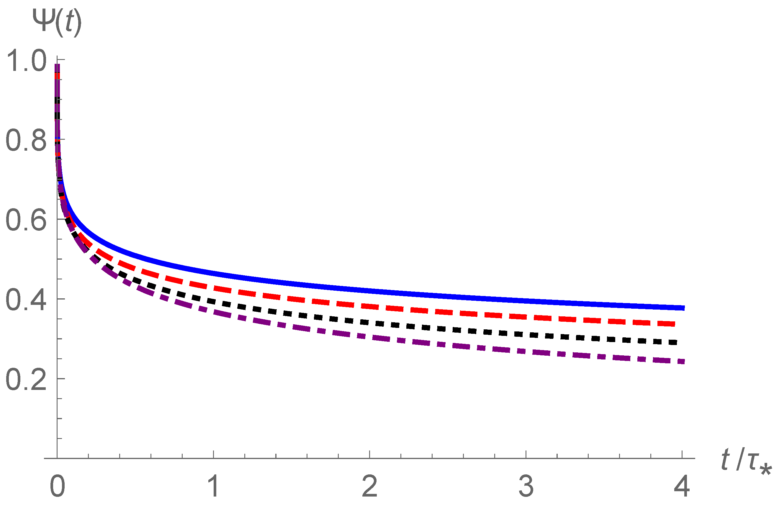
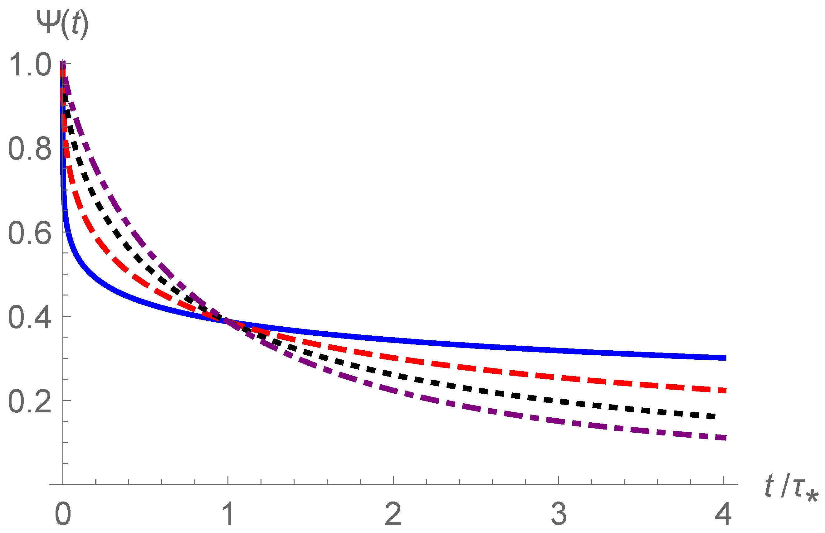
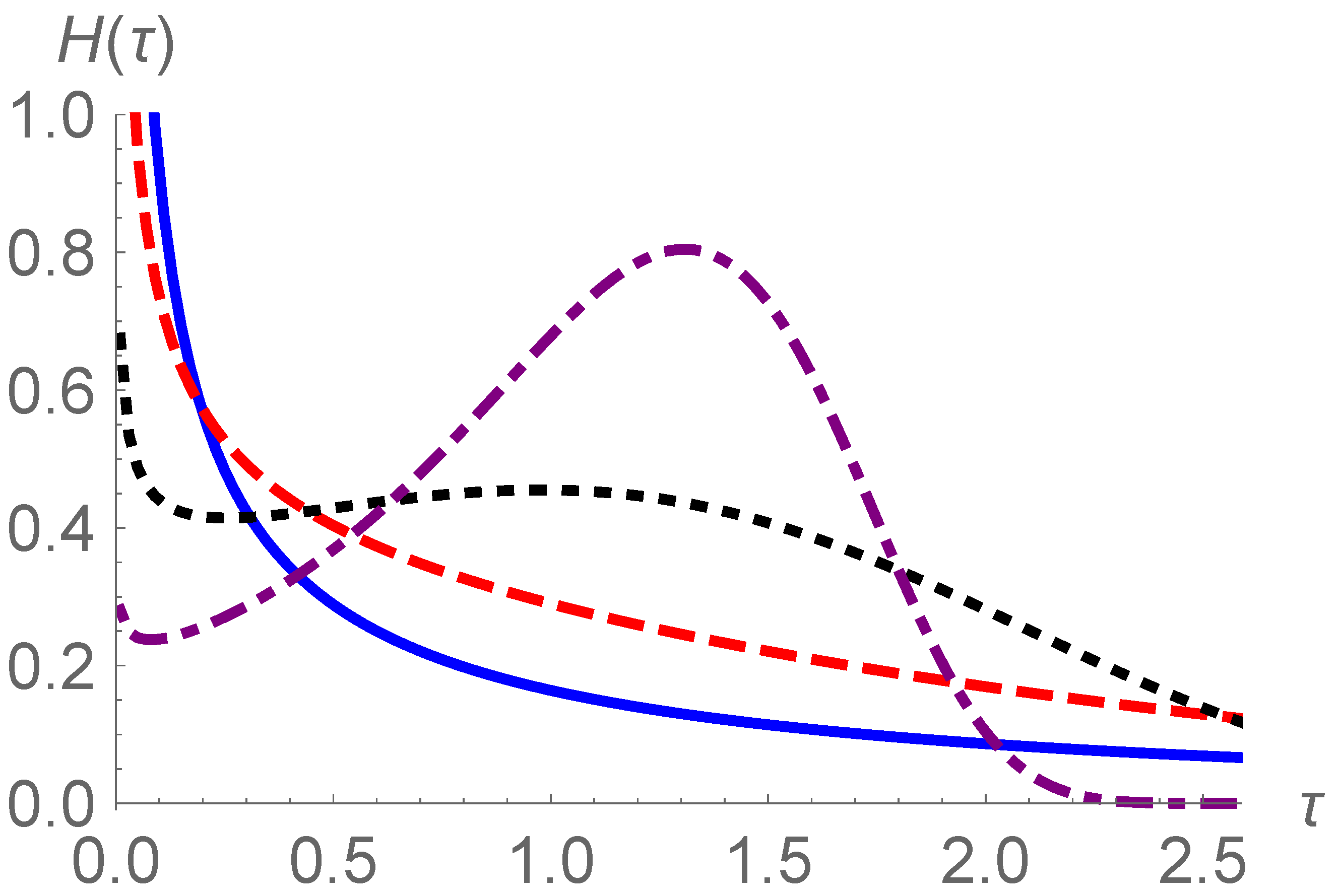
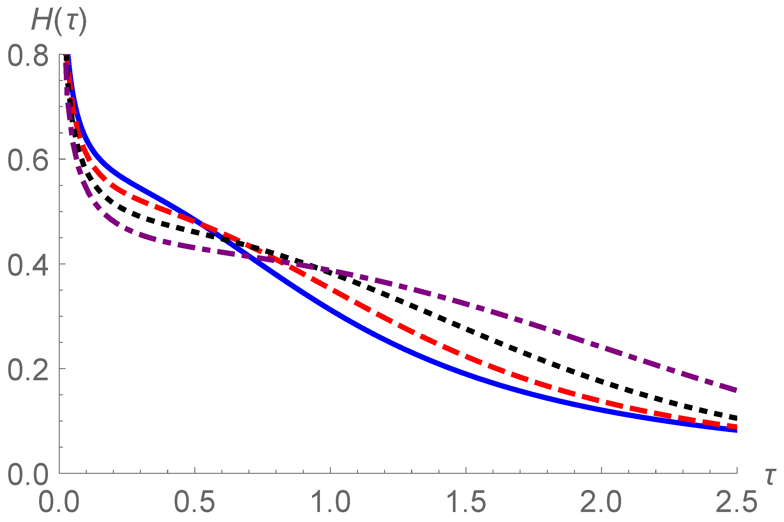
Relaxation functions $\mathsf{\Psi }\left(t\right)$ are plotted in Figure 1 for $\gamma =0.25$ and four values of $\alpha$: 0.25, 0.5, 0.75, 1, and in Figure 2 for $\alpha =0.8$ and four values of $\gamma$: 0.2, 0.4, 0.6, 0.8. A continuous shift from the CC relaxation function $\mathsf{\Psi }(t;0.25,0.25)$ to the KWW relaxation function $\mathsf{\Psi }(t;1,0.25)$ is shown in Figure 1. For the two asymptotic behaviors in Equations (18) and (19), $\alpha$ only affects coefficients, while $\gamma$ serves as the exponents of power functions of t. The apparent effects of $\gamma$ on the asymptotic behaviors are shown in Figure 2. Note that in Figure 1 and Figure 2, curves of the relaxation function $\mathsf{\Psi }\left(t\right)$ were depicted by invoking the built-in command ‘MittagLefflerE’ of the Mittag–Leffler function in Mathematica 11.3.

For the case of the CC relaxation, the Laplace transform of the relaxation function $\mathsf{\Psi }(t;\alpha ,\alpha )$ has the concise closed form as in Equation (8). However, for the general case, we only have

$$\tilde{\mathsf{\Psi }}(s;\alpha ,\gamma )=\sum _{k=0}^{\infty }\frac{{(-1)}^k\mathsf{\Gamma }(\gamma k+1)}{\mathsf{\Gamma }(\alpha k+1){\tau }_{*}^{\gamma k}{s}^{\gamma k+1}},$$

(20)

by transformation term by term for the series expansion of the Mittag–Leffler function in Equation (15). Due to the asymptotic formula on the gamma function [37]

$$\frac{\mathsf{\Gamma }(z+a)}{\mathsf{\Gamma }(z+b)}\sim z^{a-b},z\to +\infty ,$$

(21)

we know that the series in Equation (20) converges for all $\left|s\right|>0$ if $\alpha >\gamma$.

We remark that, due to the Mittag–Leffler function in the form of $t^{\beta -1}{E}_{\alpha ,\beta }(-t^{\alpha })$ and the Prabhakar function in the form of $t^{\beta -1}{E}_{\alpha ,\beta }^{\gamma }(-t^{\alpha })$ in Equations (11) and (17) have the compact and closed-form Laplace transform, they have been used in the popular fields of theory and applications of fractional calculus [18,24,34,35,36,38]. In this paper, the Mittag–Leffler function we used in Equation (15) has a complicated form in the Laplace domain in Equation (20), which is nonclosed in general. This raises difficulties in the further analysis.

3. The Response Function and the Complex Dielectric Permittivity

By Equations (6) and (10), and taking the derivatives term by term for the series expansion of the relaxation function (15), the response function is derived as

$$\varphi \left(t\right)=\varphi (t;\alpha ,\gamma )=\frac{\gamma }{\alpha {\tau }_{*}}{\left(\frac{t}{{\tau }_{*}}\right)}^{\gamma -1}{E}_{\alpha ,\alpha }\left(-{\left(\frac{t}{{\tau }_{*}}\right)}^{\gamma }\right),0<\gamma \le \alpha \le 1.$$

(22)

From the definition (10) and the asymptotic expansion (12), or from the asymptotic expressions (18) and (19), the response function has the asymptotic behaviors,

$$\begin{array}{ccc}\hfill \varphi (t;\alpha ,\gamma )& \sim & \frac{\gamma }{\mathsf{\Gamma }(1+\alpha ){\tau }_{*}}{\left(\frac{t}{{\tau }_{*}}\right)}^{\gamma -1},t\to 0^{+}.\hfill \end{array}$$

(23)

$$\begin{array}{ccc}\hfill \varphi (t;\alpha ,\gamma )& \sim & \frac{\gamma }{\mathsf{\Gamma }(1-\alpha ){\tau }_{*}}{\left(\frac{t}{{\tau }_{*}}\right)}^{-\gamma -1},t\to +\infty .\hfill \end{array}$$

(24)

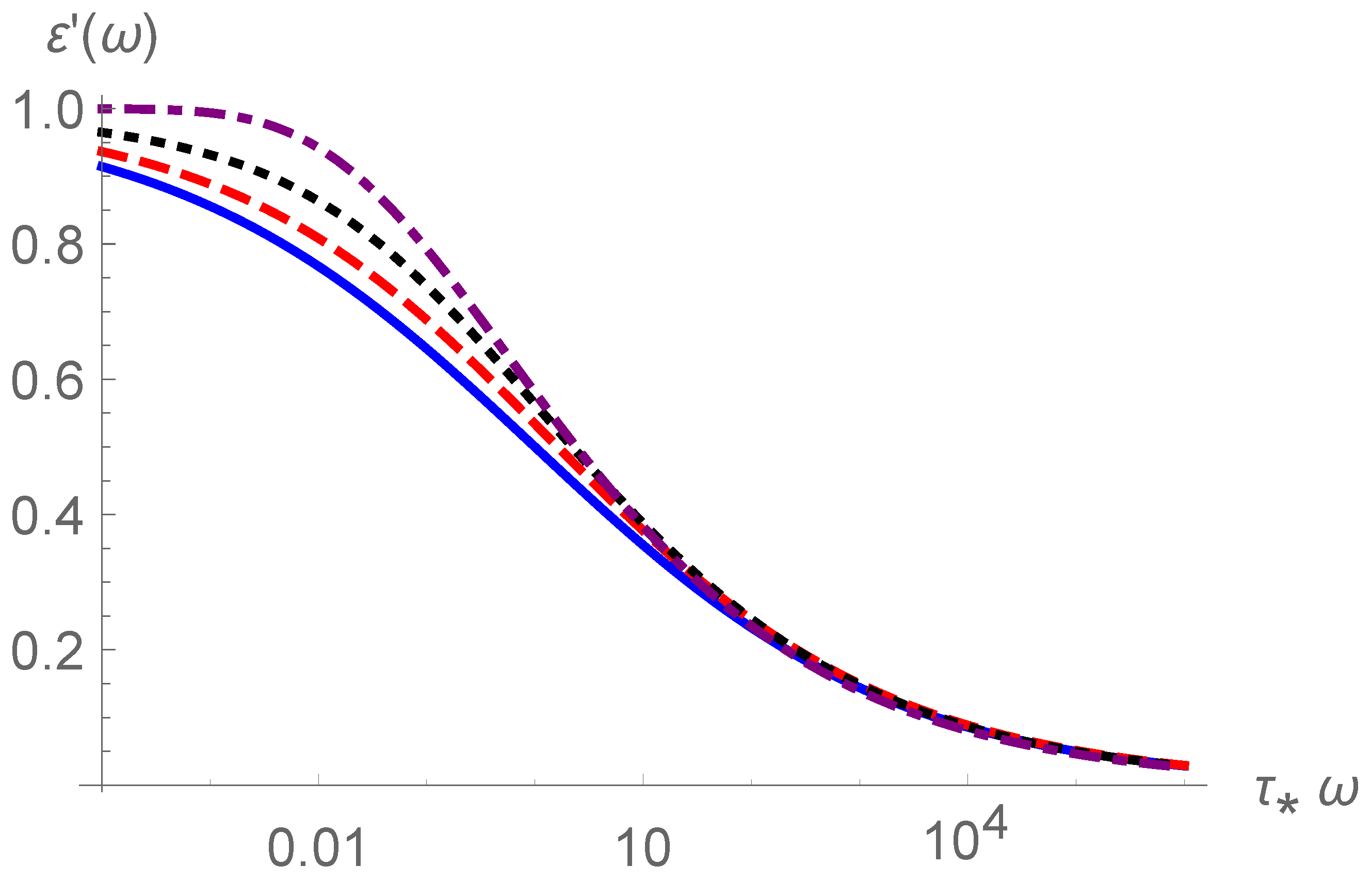
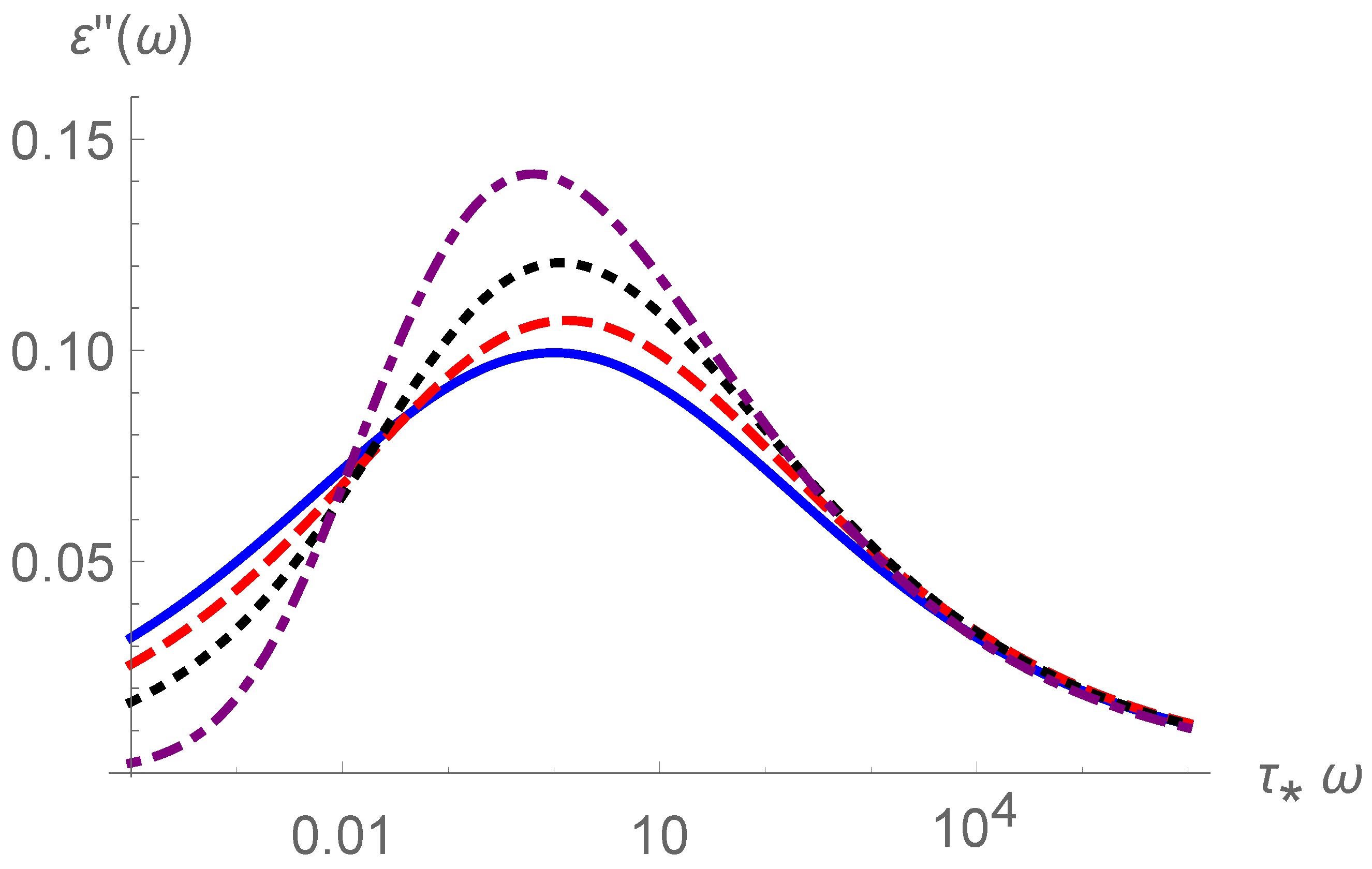
By Equations (1) and (5), the dielectric storage and loss factors, i.e., the real and imaginary parts of the normalized complex permittivity, are the Fourier cosine and sine transformations of the response function, respectively,

$$\begin{array}{c}\hfill {\epsilon }^{\prime }\left(\omega \right)={\int }_0^{\infty }\varphi \left(t\right)cos\left(\omega t\right)dt,{\epsilon }^{″}\left(\omega \right)={\int }_0^{\infty }\varphi \left(t\right)sin\left(\omega t\right)dt.\end{array}$$

(25)

By utilizing the relaxation function in Equation (6), they have the expressions

$${\epsilon }^{\prime }\left(\omega \right)=1-\omega {\int }_0^{\infty }\mathsf{\Psi }\left(t\right)sin\left(\omega t\right)dt,{\epsilon }^{″}\left(\omega \right)=\omega {\int }_0^{\infty }\mathsf{\Psi }\left(t\right)cos\left(\omega t\right)dt.$$

(26)

Substituting the proposed relaxation function in Equation (15) and letting $t/{\tau }_{*}=\zeta$, we obtain

$$\begin{array}{ccc}\hfill {\epsilon }^{\prime }\left(\omega \right)& =& 1-{\tau }_{*}\omega {\int }_0^{\infty }{E}_{\alpha ,1}(-{\zeta }^{\gamma })sin\left({\tau }_{*}\omega \zeta \right)d\zeta ,\hfill \end{array}$$

(27)

$$\begin{array}{ccc}\hfill {\epsilon }^{″}\left(\omega \right)& =& {\tau }_{*}\omega {\int }_0^{\infty }{E}_{\alpha ,1}(-{\zeta }^{\gamma })cos\left({\tau }_{*}\omega \zeta \right)d\zeta .\hfill \end{array}$$

(28)

Equations (27) and (28) enable us to conveniently simulate the dielectric storage and loss factors for specified $\alpha$ and $\gamma$. Storage factor and loss factor against ${\tau }_{*}\omega$ are plotted in Figure 3 and Figure 4, respectively, for $\gamma =0.25$ and four values of $\alpha$: 0.25, 0.5, 0.75, 1, where transitions from the CC model ($\alpha =\gamma =0.25$, solid lines) to the KWW model ($\alpha =1$ and $\gamma =0.25$, dot–dash lines) are shown. Distinct effects of the varying $\alpha$ are displayed in the low-frequency range in both figures and in the range where dielectric loss peaks appear, as shown in in Figure 4. Note that Figure 3 and Figure 4 were generated using Equations (27) and (28) and the Mathematica numerical integration command ‘NIntegrate’.

The series expression of the complex permittivity can be obtained by considering Equations (7) and (20) as

$$\widehat{\epsilon }\left(s\right)=\sum _{k=1}^{\infty }\frac{{(-1)}^{k-1}\mathsf{\Gamma }(\gamma k+1)}{\mathsf{\Gamma }(\alpha k+1){\left({\tau }_{*}s\right)}^{\gamma k}}.$$

(29)

Inserting $s=\mathrm{i}\omega$ and separating the real and imaginary parts, we obtain the series expressions for the dielectric storage and loss factors

$$\begin{array}{ccc}\hfill {\epsilon }^{\prime }\left(\omega \right)& =& \sum _{k=1}^{\infty }\frac{{(-1)}^{k-1}\mathsf{\Gamma }(\gamma k+1)}{\mathsf{\Gamma }(\alpha k+1){\left({\tau }_{*}\omega \right)}^{\gamma k}}cos\left(\frac{\pi }{2}\gamma k\right),\hfill \end{array}$$

(30)

$$\begin{array}{ccc}\hfill {\epsilon }^{″}\left(\omega \right)& =& \sum _{k=1}^{\infty }\frac{{(-1)}^{k-1}\mathsf{\Gamma }(\gamma k+1)}{\mathsf{\Gamma }(\alpha k+1){\left({\tau }_{*}\omega \right)}^{\gamma k}}sin\left(\frac{\pi }{2}\gamma k\right).\hfill \end{array}$$

(31)

Due to the asymptotic formula (21), the series in Equations (30) and (31) converge for all ${\tau }_{*}\omega >0$ if $\gamma <\alpha$, while converging for ${\tau }_{*}\omega >1$ if $\gamma =\alpha$. In fact, if $\gamma =\alpha$, i.e., for the CC relaxation, the closed forms of the dielectric storage and loss factors can be obtained from Equations (7) and (8) as [12]

$$\begin{array}{ccc}\hfill {\epsilon }^{\prime }(\omega ;\alpha ,\alpha )& =& \frac{1+{\tau }_{*}^{\alpha }{\omega }^{\alpha }cos(\pi \alpha /2)}{{\tau }_{*}^{2\alpha }{\omega }^{2\alpha }+2{\tau }_{*}^{\alpha }{\omega }^{\alpha }cos(\pi \alpha /2)+1},\hfill \end{array}$$

(32)

$$\begin{array}{ccc}\hfill {\epsilon }^{″}(\omega ;\alpha ,\alpha )& =& \frac{{\tau }_{*}^{\alpha }{\omega }^{\alpha }sin(\pi \alpha /2)}{{\tau }_{*}^{2\alpha }{\omega }^{2\alpha }+2{\tau }_{*}^{\alpha }{\omega }^{\alpha }cos(\pi \alpha /2)+1}.\hfill \end{array}$$

(33)

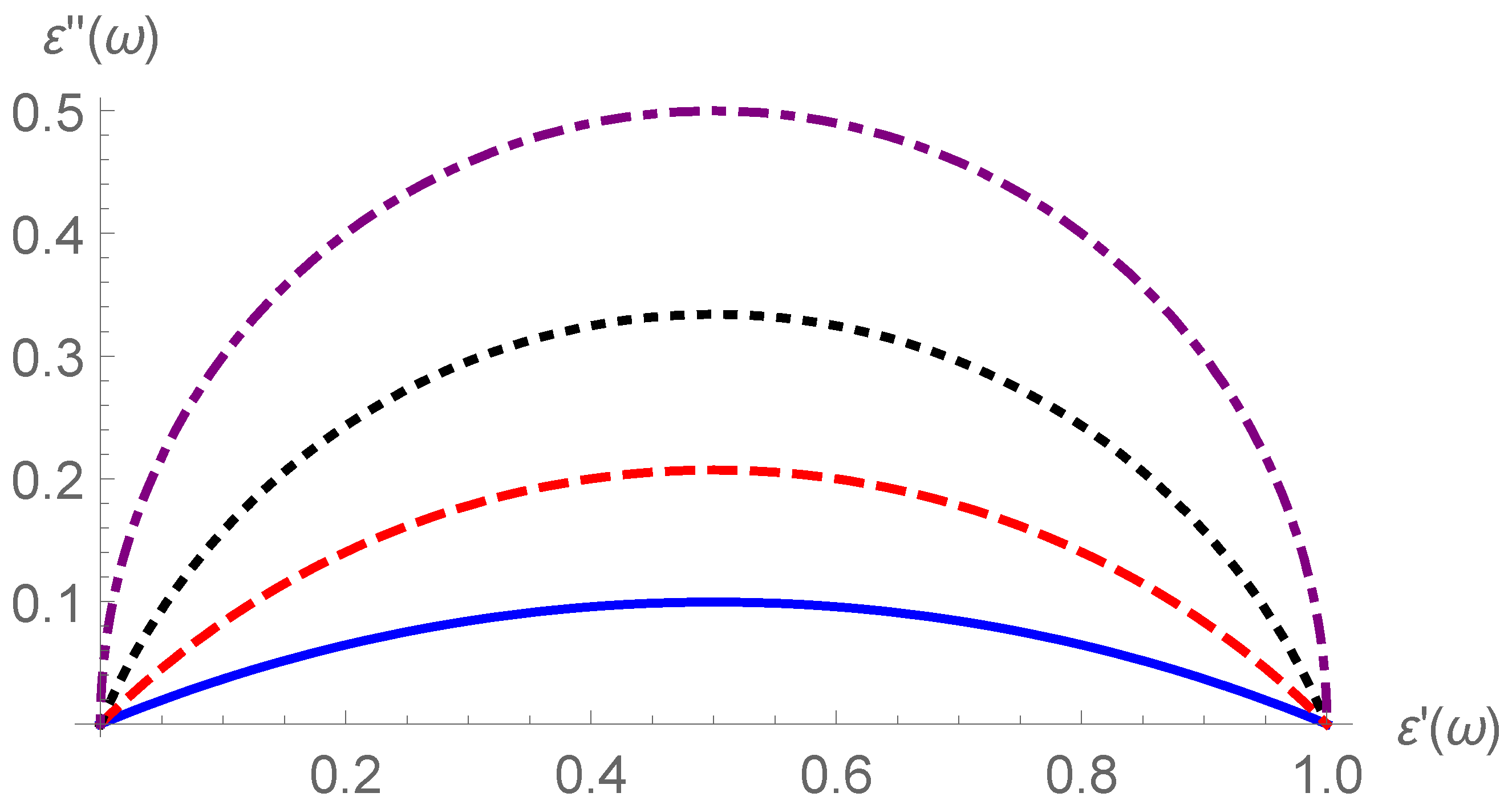
It is easy to verify that the dielectric storage and loss factors of the CC relaxation satisfy the equation of the circle

$${\left({\epsilon }^{\prime }(\omega ;\alpha ,\alpha )-\frac{1}{2}\right)}^2+{\left({\epsilon }^{″}(\omega ;\alpha ,\alpha )+\frac{1}{2tan\left(\pi \alpha /2\right)}\right)}^2=\frac{1}{4{sin}^2\left(\pi \alpha /2\right)}.$$

(34)

The Cole–Cole plot of a relaxation model is a useful tool for analyzing relaxatory modes from experimental data [3]. As $\omega$ increases from 0 to $+\infty$, the Cole–Cole plot of the CC relaxation is a circular arc with the starting point $(1,0)$ and terminal limit (0,0), whose center is the point $\left(\frac{1}{2},-\frac{1}{2tan\left(\pi \alpha /2\right)}\right)$ and the radius is $\frac{1}{2sin\left(\pi \alpha /2\right)}$. 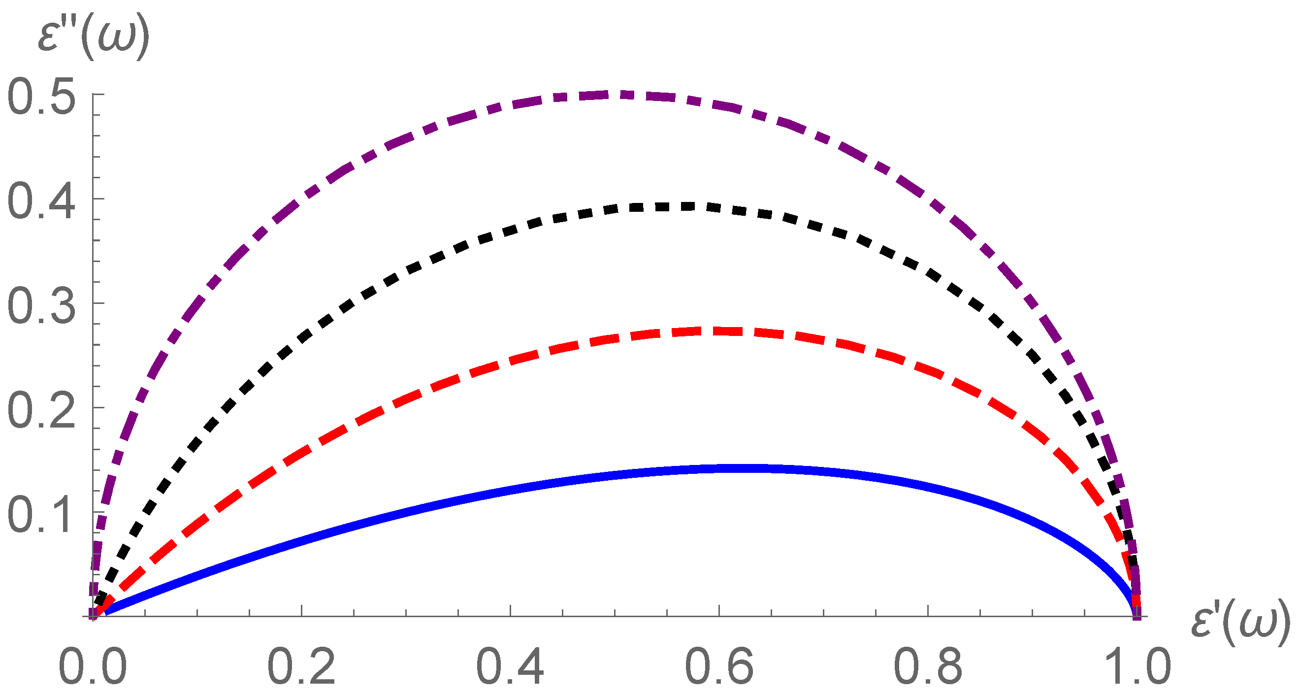The Cole–Cole plots of the CC relaxation and KWW relaxation are shown in Figure 5 and Figure 6, respectively, where the arcs for $\alpha =1$ in Figure 5 and for $\gamma =1$ in Figure 6 are semicircles corresponding to the Debye relaxation. Usually, the Debye relaxation is identified by observing whether the Cole–Cole plot is a semicircle. 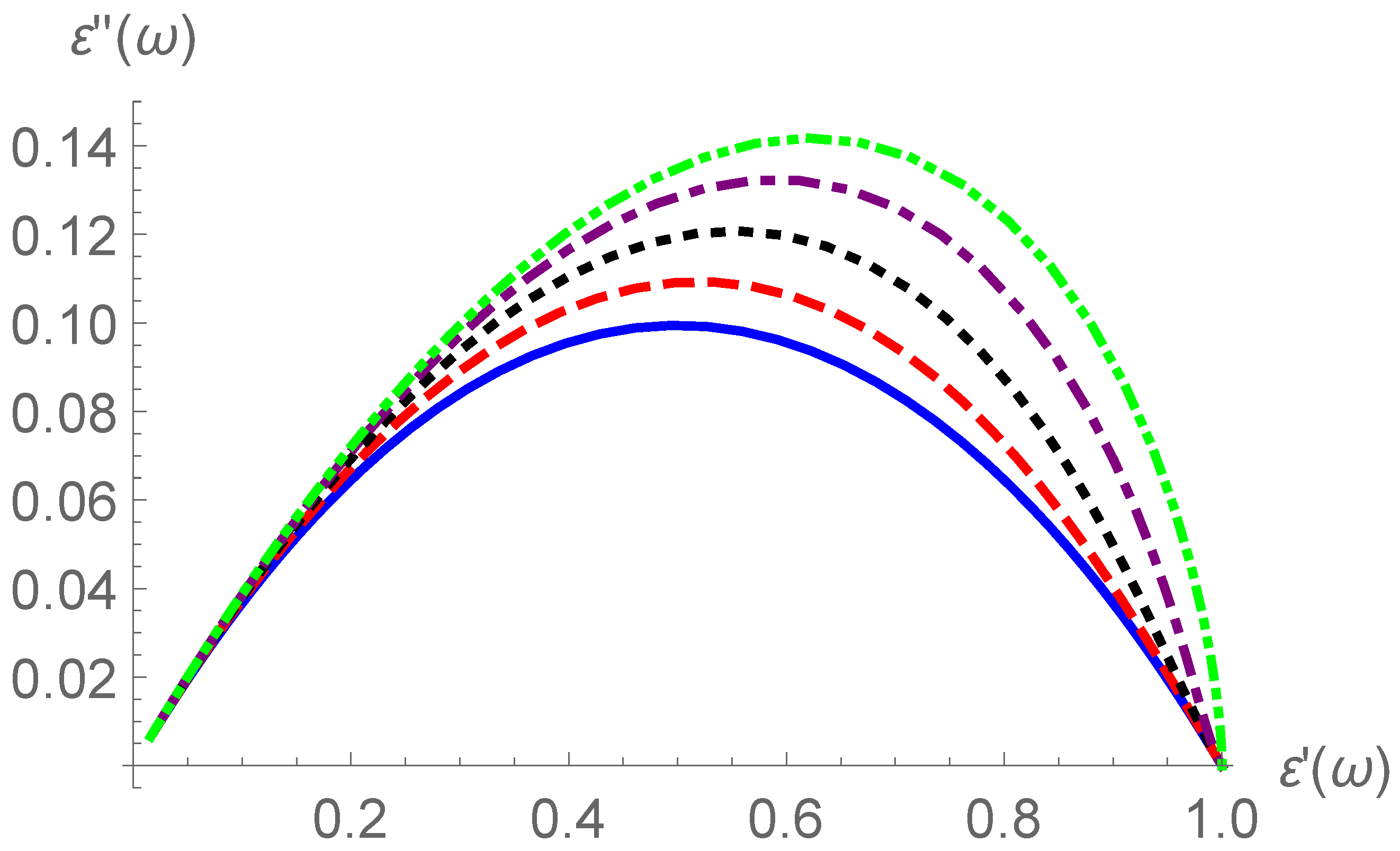In practice, Cole–Cole plots deviating from the semicircle exist extensively [1,2,3]. In Figure 7, Cole–Cole plots for $\gamma =0.25$ and five values of $\alpha$ from 0.25 to 1 are shown, where curves display a shift from the case of the CC relaxation ($\alpha =\gamma =0.25$, solid line) to that of the KWW relaxation ($\alpha =1$ and $\gamma =0.25$, dot–dot–dash line). Note that Figure 5 is depicted using Equation (34), while Figure 6 and Figure 7 use data computed from Equations (27) and (28).

For the CC relaxation, the Cole–Cole plot is a symmetric circular arc, while for the KWW relaxation, it is asymmetric and has a rightward loss peak. A transition between the two cases was displayed in Figure 7. Note that the Cole–Cole plots are commonly used to analyze experimental data and inspect theoretical models. In [39], dynamic properties of a sort of polypropylene composites were investigated based on the Cole–Cole plot analysis. In [40], Cole–Cole plots were used to analyze the viscoelastic and mechanical properties of smart thermoplastic elastomeric materials based on recycled rubber shred.

The gradients of the Cole–Cole plots at the starting and terminal points are determined by the asymptotic behaviors of the complex permittivity. From Equations (30) and (31), the asymptotic behaviors for large $\omega$ are obtained

$$\begin{array}{ccc}\hfill {\epsilon }^{\prime }\left(\omega \right)& \sim & \frac{\mathsf{\Gamma }(1+\gamma )}{\mathsf{\Gamma }(1+\alpha )}cos\left(\frac{\pi \gamma }{2}\right){\left({\tau }_{*}\omega \right)}^{-\gamma },{\tau }_{*}\omega \to +\infty ,\hfill \end{array}$$

(35)

$$\begin{array}{ccc}\hfill {\epsilon }^{″}\left(\omega \right)& \sim & \frac{\mathsf{\Gamma }(1+\gamma )}{\mathsf{\Gamma }(1+\alpha )}sin\left(\frac{\pi \gamma }{2}\right){\left({\tau }_{*}\omega \right)}^{-\gamma },{\tau }_{*}\omega \to +\infty .\hfill \end{array}$$

(36)

Taking the Laplace transforms for the asymptotic expressions for a large t in Equation (19) or (24), and then using Equation (5) or (7), we obtain the asymptotic behaviors for small $\omega$,

$$\begin{array}{ccc}\hfill {\epsilon }^{\prime }\left(\omega \right)& \sim & 1-\frac{\mathsf{\Gamma }(1-\gamma )}{\mathsf{\Gamma }(1-\alpha )}cos\left(\frac{\pi \gamma }{2}\right){\left({\tau }_{*}\omega \right)}^{\gamma },{\tau }_{*}\omega \to 0^{+},\hfill \end{array}$$

(37)

$$\begin{array}{ccc}\hfill {\epsilon }^{″}\left(\omega \right)& \sim & \frac{\mathsf{\Gamma }(1-\gamma )}{\mathsf{\Gamma }(1-\alpha )}sin\left(\frac{\pi \gamma }{2}\right){\left({\tau }_{*}\omega \right)}^{\gamma },{\tau }_{*}\omega \to 0^{+},\hfill \end{array}$$

(38)

where $\alpha$ and $\gamma$ cannot simultaneously be 1.

From Equations (35) and (36), the left dip angle of the Cole–Cole arc corresponding to $\omega \to +\infty$ is $\pi \gamma /2$ for all $0<\alpha \le 1.$ From Equations (37) and (38), the right dip angle of the Cole–Cole arc corresponding to $\omega \to 0^{+}$ is also $\pi \gamma /2$ for $0<\alpha <1.$

For $\alpha =1$, the asymptotic expressions (37) and (38) only yield ${\epsilon }^{\prime }\sim 1$ and ${\epsilon }^{″}\sim 0$ as $\omega \to 0^{+}$. For a more detailed analysis for the KWW case of $\alpha =1$, we take one-term Taylor approximations of $sin\left({\tau }_{*}\omega \zeta \right)$ and $cos\left({\tau }_{*}\omega \zeta \right)$ in Equations (27) and (28), and then obtain more accurate asymptotic estimations as

$$\begin{array}{ccc}\hfill {\epsilon }^{\prime }(\omega ;1,\gamma )& \sim & 1-\frac{1}{2}\mathsf{\Gamma }\left(1+\frac{2}{\gamma }\right){\left({\tau }_{*}\omega \right)}^2,{\tau }_{*}\omega \to 0^{+},\hfill \end{array}$$

(39)

$$\begin{array}{ccc}\hfill {\epsilon }^{″}(\omega ;1,\gamma )& \sim & \mathsf{\Gamma }\left(1+\frac{1}{\gamma }\right){\tau }_{*}\omega ,{\tau }_{*}\omega \to 0^{+}.\hfill \end{array}$$

(40)

This indicates that, for the KWW model ($\alpha =1$), the right dip angle of the Cole–Cole arc corresponding to $\omega \to 0^{+}$ is always $\pi /2$. This feature is shown in Figure 6.

4. Relaxation Frequency and Time Spectral Functions

Relaxation frequency and time spectral functions, $K\left(r\right),r>0$ and $H\left(\tau \right),\tau >0$, are defined as

$$\mathsf{\Psi }\left(t\right)={\int }_0^{\infty }{e}^{-rt}K\left(r\right)dr,\mathsf{\Psi }\left(t\right)={\int }_0^{\infty }{e}^{-t/\tau }H\left(\tau \right)d\tau .$$

(41)

That is, the relaxation function $\mathsf{\Psi }\left(t\right)$ is the real Laplace transform of the frequency spectral function $K\left(r\right)$, and the time spectral function has the expression by the replacement $r=1/\tau$,

$$H\left(\tau \right)=\frac{1}{{\tau }^2}K\left(\frac{1}{\tau }\right),\tau >0.$$

(42)

This implies the symmetrical relation between the two spectral functions,

$$\tau H\left(\tau \right)=rK\left(r\right),\tau r=1.$$

Note that the complete monotonicity of the relaxation function $\mathsf{\Psi }\left(t\right)$ ensures the existence of non-negative spectral functions. From Equations (7) and (41), and the relations ${\int }_0^{\infty }K\left(r\right)dr={\int }_0^{\infty }H\left(\tau \right)d\tau =1$, the complex permittivity has the spectral representations,

$$\widehat{\epsilon }\left(\mathrm{i}\omega \right)={\int }_0^{\infty }\frac{1}{1+\mathrm{i}(1/r)\omega }K\left(r\right)dr={\int }_0^{\infty }\frac{1}{1+\mathrm{i}\tau \omega }H\left(\tau \right)d\tau .$$

(43)

For the Debye relaxation ($\alpha =\gamma =1$), the spectral functions are the Dirac delta functions $K\left(r\right)=\delta (r-\frac{1}{{\tau }_{*}})$ and $H\left(\tau \right)=\delta (\tau -{\tau }_{*})$. Below, we assume that $\alpha$ and $\gamma$ are not equal to 1 at the same time, i.e., $0<\gamma <1$.

By the complex inverse formula of the Laplace transform along the Bromwich path, the frequency spectral function has the integral expression

$$\begin{array}{ccc}\hfill K\left(r\right)& =& \frac{-1}{\pi }{\int }_0^{\infty }\mathrm{Im}\left[\mathsf{\Psi }\left(u{e}^{i\pi }\right)\right]e^{-ur}du.\hfill \end{array}$$

(44)

Alternatively, by iterating the inverse Laplace transform of $\tilde{\mathsf{\Psi }}\left(s\right)$, Equation (44) becomes

$$K\left(r\right)=\frac{-1}{\pi }\mathrm{Im}\left[\tilde{\mathsf{\Psi }}\left(r{e}^{i\pi }\right)\right].$$

(45)

Thus, by Equation (42), the time spectral function has the form

$$H\left(\tau \right)=\frac{-1}{\pi {\tau }^2}{\int }_0^{\infty }\mathrm{Im}\left[\mathsf{\Psi }\left(u{e}^{i\pi }\right)\right]e^{-u/\tau }du,$$

(46)

or

$$H\left(\tau \right)=\frac{-1}{\pi {\tau }^2}\mathrm{Im}\left[\tilde{\mathsf{\Psi }}\left(\frac{1}{\tau }{e}^{i\pi }\right)\right].$$

(47)

Applying Equations (20), (45) and (47), the series expressions of the frequency and time spectral functions are derived as

$$\begin{array}{c}\hfill K\left(r\right)=\frac{1}{r}\sum _{k=1}^{\infty }\frac{{(-1)}^k{\left({\tau }_{*}r\right)}^{-\gamma k}}{\mathsf{\Gamma }(\alpha k+1)\mathsf{\Gamma }(-\gamma k)},\end{array}$$

(48)

and

$$\begin{array}{c}\hfill H\left(\tau \right)=\frac{1}{{\tau }_{*}}\sum _{k=1}^{\infty }\frac{{(-1)}^k}{\mathsf{\Gamma }(\alpha k+1)\mathsf{\Gamma }(-\gamma k)}{\left(\frac{\tau }{{\tau }_{*}}\right)}^{\gamma k-1}.\end{array}$$

(49)

For the case of $\gamma <\alpha$, the series in Equations (48) and (49) converge for all $r>0$ and $\tau >0$, respectively, due to the reflection and asymptotic formulas on the gamma function. We note that, in [35], the spectral distribution of a relaxation model involving the Prabhakar function was derived and its condition of non-negativity was given.

For the special case $\alpha =\gamma$ of the CC relaxation, the spectral functions have closed forms from Equations (8), (45) and (47),

$$K(r;\alpha ,\alpha )=\frac{{\tau }_{*}}{\pi }\frac{{\left({\tau }_{*}r\right)}^{\alpha -1}sin\left(\pi \alpha \right)}{{\left({\tau }_{*}r\right)}^{2\alpha }+2{\left({\tau }_{*}r\right)}^{\alpha }cos\left(\pi \alpha \right)+1},$$

(50)

$$H(\tau ;\alpha ,\alpha )=\frac{1}{\pi {\tau }_{*}}\frac{{(\tau /{\tau }_{*})}^{\alpha -1}sin\left(\pi \alpha \right)}{{(\tau /{\tau }_{*})}^{2\alpha }+2{(\tau /{\tau }_{*})}^{\alpha }cos\left(\pi \alpha \right)+1}.$$

(51)

Note that this result was obtained by Gorenflo and Mainardi [41].

For the special case $\alpha =1$ of the KWW relaxation, the two spectral functions in (48) and (49) do not have closed forms in general. However, for the fraction $\gamma =1/2$, there are simplified forms as

$$K(r;1,1/2)=\frac{1}{2\sqrt{\pi }r\sqrt{{\tau }_{*}r}}{e}^{-\frac{1}{4{\tau }_{*}r}},H(\tau ;1,1/2)=\frac{1}{2\sqrt{\pi }{\tau }_{*}}\sqrt{\frac{{\tau }_{*}}{\tau }}{e}^{-\frac{\tau }{4{\tau }_{*}}}.$$

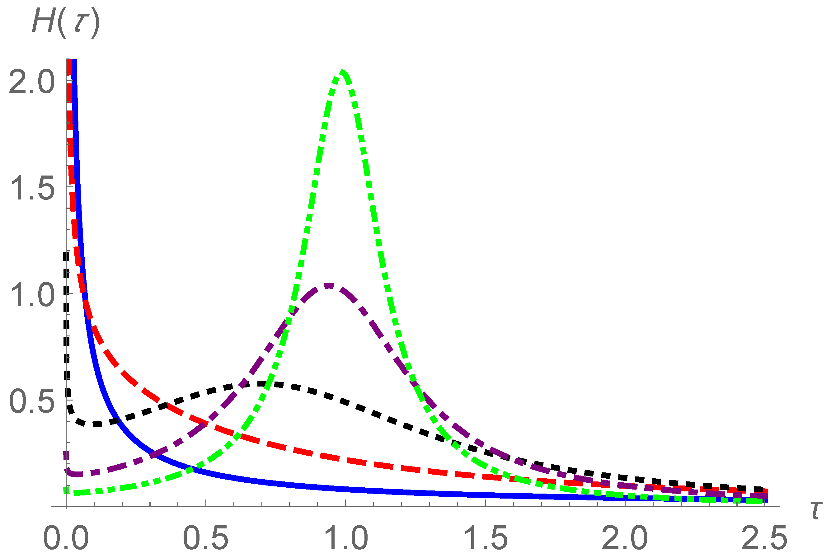
We use these results to simulate the time spectral functions. From Equation (49), we have

$$H\left(\tau \right)\sim \frac{\gamma }{{\tau }_{*}\mathsf{\Gamma }(\alpha +1)\mathsf{\Gamma }(1-\gamma )}{\left(\frac{\tau }{{\tau }_{*}}\right)}^{\gamma -1},\tau \to 0^{+}.$$

The time spectral functions $H(\tau ;\alpha ,\alpha )$ of the CC relaxation are plotted in Figure 8 for five specified values of $\alpha$. The spectral functions $H(\tau ;1,\gamma )$ of the KWW relaxation are shown in Figure 9 for four specified values of $\gamma$. Time spectral functions only display peaks when both $\alpha$ and $\gamma$ approach 1. In Figure 10, a transition of spectral functions from the CC case $H(\tau ;0.7,0.7)$ to the KWW case $H(\tau ;1,0.7)$ is shown. The time spectral functions of the CC relaxation surpass that of the KWW relaxation in an initial phase of $\tau$, but then, for a larger $\tau$, the superiority yields to the KWW relaxation. Note that Figure 8 was depicted based on Equation (51), while Figure 9 and Figure 10 were generated using data computed from Equation (46).

5. Discussion

In the time domain, we propose a relaxation function with two parameters besides a relaxation time, having a concise form in terms of the Mittag–Leffler function

$$\mathsf{\Psi }(t;\alpha ,\gamma )=E_{\alpha ,1}\left(-{\left(\frac{t}{{\tau }_{*}}\right)}^{\gamma }\right),0<\gamma \le \alpha \le 1.$$

The relaxation model simplifies to the CC model if $\alpha =\gamma$ and to the KWW model if $\alpha =1$. The case $\alpha =\gamma =1$ becomes the Debye relaxation.

The proposed relaxation function interpolates the CC and the KWW relaxation models, and is proven to be complete monotonic. Thus, it is acceptable in physics. However, unlike in the case of the CC relaxation, where the relaxation function has the Laplace transform in a closed form in Equation (8), which also leads to closed forms for dielectric storage and loss factors in Equations (32) and (33), and for relaxation spectral functions in Equations (50) and (51), the built-in commands ‘MittagLefflerE’ and ‘NIntegrate’ in Mathematica 11.3 for the computation of the Mittag–Leffler function and its integration enable us to simulate the obtained results conveniently using Equations (15), (22), (27), (28), (44) and (46). All figures were generated in Mathematica 11.3. In addition, using the series expression (10) and the asymptotic expansion (12) of the Mittag–Leffler function, the asymptotic behaviors of the relaxation function, response function and dielectric storage and loss factors are derived as in Equations (18), (19), (23), (24) and (35)–(38).

For the Cole–Cole plots in Figure 5, Figure 6 and Figure 7, in the CC relaxation, symmetrical circular arcs are shown; in the KWW relaxation, loss peaks moving to the right are displayed with orthogonal right dip angles; while for the general case $0<\gamma <\alpha <1$, loss peaks appear rightward with symmetrical left and right dip angles. From the asymptotic behaviors of the dielectric storage and loss factors in Equations (35)–(38), the proposed relaxation model in the case of $\alpha <1$ satisfies the Jonscher’s universal relaxation law in Equations (3) and (4), where power exponents m and n are characterized by our model parameter $\gamma$ as $m=\gamma$ and $n=1-\gamma$.

Although the proposed relaxation function has a concise form in terms of the two-parameter Mittag–Leffler function, responses in the frequency domain do not have a closed form in general and the peaks of Cole–Cole plots always move to the right relative to the symmetrical CC model. These are limitations of the considered model. We mention that the Havriliak–Negami model has advantages in these aspects [5,7].

6. Conclusions

The proposed relaxation function in terms of the Mittag–Leffler function has a concise form, can be computed conveniently, interpolates the CC model and the KWW model through varying of parameters $\alpha$ and $\gamma$, and is proven to be complete monotonic. The response function is also expressed in terms of the Mittag–Leffler function. Starting from the two causal functions in the time domain, the relaxation function and response function, we derive the integral and series expressions for the normalized complex dielectric permittivity, dielectric storage and loss factors and the relaxation frequency and time spectral functions. These results facilitate numerical simulations and are potentially applied to the polarization analysis of complex dielectric materials.