Solving Fractional Order Differential Equations by Using Fractional Radial Basis Function Neural Network

Abstract

Fractional differential equations (FDEs) arising in engineering and other sciences describe nature sufficiently in terms of symmetry properties. This paper proposes a numerical technique to approximate ordinary fractional initial value problems by applying fractional radial basis function neural network. The fractional derivative used in the method is considered Riemann-Liouville type. This method is simple to implement and approximates the solution of any arbitrary point inside or outside the domain after training the ANN model. Finally, three examples are presented to show the validity and applicability of the method.

1. Introduction

The symmetry design of the system includes integer partial differential equations and fractional-order partial differential equations. Fractional differential equations (FDEs) can be applied for modelling many problems in real-life. Lately, fractional calculus has received much consideration of the researchers due to it’s numerous applications in diverse scientific fields such as fluid flow, dynamical system control theory, signal processing, diffusion transport, electric network, etc. [1,2,3,4]. In most cases, it is hard to gain analytical solutions of these problems. Therefore, numerical approaches have to be applied for approximating the solution of FDEs [5,6,7,8,9,10,11,12,13,14,15].

According to our primary studies, over the past decades, various numerical methods have been proposed for solving these problems. For example finite difference [16,17], Adomian decomposition [18], monotone iterative technique [19], random walk [20], operational matrix method [21,22], etc. Although these techniques provide good approximations to the solution, but most of them give series expansions in the neighborhood of initial conditions are used [23].

In recent years, artificial neural network (ANN ) methods have been established as a powerful technique to solve partial and ordinary differential problems [24,25,26].

Lagaris et al. [27] proposed an artificial neural network method to solve boundary and initial value problems. Pakdaman et al. [28] applied neural network and Broyden-Fletcher-Goldfarb-Shanno (BFGS) optimization technique to solve linear and nonlinear FDEs. Pang et al. [29] presented fractional physics-informed neural networks to solve space-time fractional advection-diffusion equations. Jafarian et al. [30] employed ANN model for approximate polynomial solution of fractional order Volterra integro differential equations. Qu et al. [31] discussed about a neural network algorithm based on Legendre’s polynomial to solve fractional diffusion equations. In another study, the neural network training and cosine basis functions with adjustable parameters have been presented by Qu and Liu for solving fractional order differential equations [32].

One of the advantages of solving equations ANN is the simple implementation and approximation of the solution of any desired point inside or outside the domain after training the ANN model. In this paper, we apply fractional radial basis function neural network (FRBF-NN) to solve fractional order initial value problems.

This paper is organized as follows: Section 2 lists basis definitions and fundamental issues of fractional calculus and structure of RBF neural network are given. Section 3 describes the proposed algorithm for solving FDEs. Section 4 presents three examples to show the effectiveness of the proposed method. Finally, Section 5 includes the concluding remarks.

2. Preliminaries

In this section, we intend to give some definitions and concepts related to fractional calculus and RBF neural network, which are used further in this article.

2.1. Fractional Derivative Definition

An important benefit of the fractional derivative over the ordinary derivative is that it extends the search region around the test point in specified boundaries [1].

The Riemann-Liouville differential operator $D^{\nu }$, for a function $f:(0,\infty )\to R$ that $\nu >0$ is defined as [33]:

$$D^{\nu }f\left(x\right)=\frac{1}{\mathsf{\Gamma }(n-\nu )}\frac{{\partial }^n}{\partial x^n}{\int }_0^x{(x-t)}^{n-\nu -1}f\left(t\right)dt,$$

(1)

that $n=\left[\nu \right]+1$, $\left[\nu \right]$ is the integer part of $\nu$ and $\mathsf{\Gamma }(.)$ denotes the Gamma function.

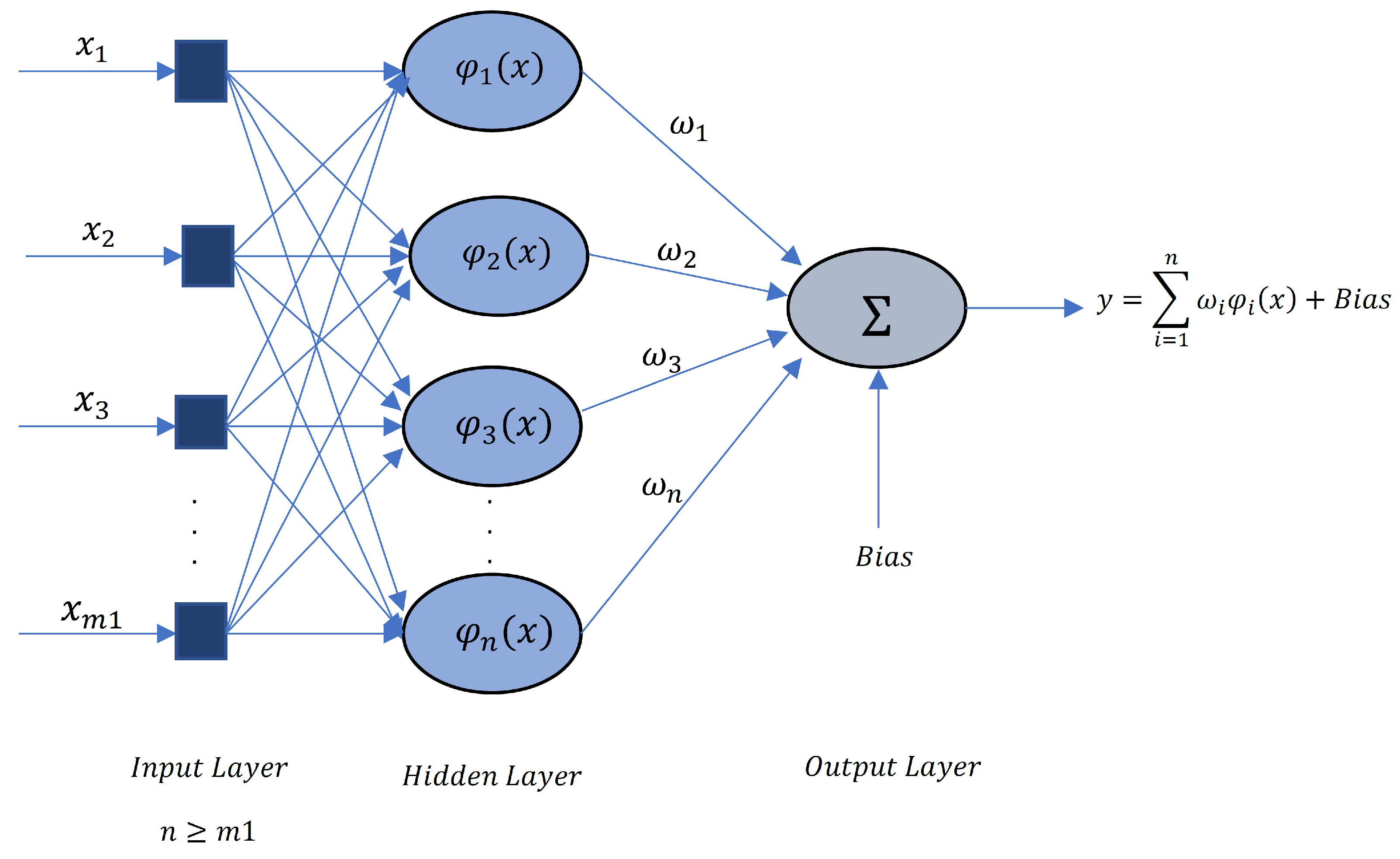
2.2. Structure of RBF-Neural Network

The RBF neural networks, can be used function approximation problems.

RBF networks architecture consists of three layers:

• The input layer
• The hidden layer includes radial basis functions:

The nonlinear input space is represented by a nonlinear mapping to a higher dimensional space in the hidden layer.

• The output layer consists of linear neurons:

Linear regression is performed to predict the desired goals by output layer. Architecture of RBF networks is indicated in Figure 1. Suppose $X\in R^{m_1}$ be the input vector, the RBF network’s overall mapping, $s:R^{m_1}\to R$ is given as:

$$y=\sum _{i=1}^M{w}_i{\varphi }_i(\parallel x-x_i\parallel )+b,$$

(2)

where M is the number of hidden layer neurons, $x_i\in R^{m_1}$ are the RBF neural network centers, $w_i$ refer to the weights between the output neuron and the hidden layer, ${\varphi }_i$ is the ith hidden neuron kernel and b refers to the bias term of the output neuron.

Without losing the generality, only one neuron is considered in the output layer. Some of the kernel functions that use in RBF neural networks are: inverse multiquadrics, multiquadrics and Gaussian functions [34]. The Gaussian function is the most commonly used kernel because of its versatility [35].

$${\varphi }_i(\parallel x-x_i\parallel )=exp(-\frac{\parallel x-x_i{\parallel }^2}{{\sigma }^2}),$$

(3)

that $\sigma$ refers to the spread of the Gaussian kernel.

3. Description of the Method

Here, we describe the fractional RBF neural network to approximate FDEs. The RBF-NN standard learning algorithms are based on classic gradient descent algorithm. By applying fractional derivatives, more information can be obtained in comparison with the classic derivative, which only results the tangent at a point of the given function [36].

Consider a FDE of order $\nu$,

$$D_x^{\nu }y\left(x\right)=f(x,y\left(x\right)),$$

where $y\left(x_0\right)=y_0,x\in R^{m_1}$.

The overall mapping, at the nth learning iteration is written as follows:

$$y\left(n\right)=\sum _{i=1}^M{w}_i\left(n\right){\varphi }_i(x,x_i)+b\left(n\right),$$

where M is the number of neurons, weights $w_i\left(n\right)$ and $b\left(n\right)$ are adjusted at each iteration. The approximate solution $y\left(n\right)$ satisfies the initials conditions.

The error function can be written as:

$$E\left(n\right)=\frac{1}{2}{(Y\left(n\right)-y\left(n\right))}^2=\frac{1}{2}\sum _k{e}_k^2\left(n\right),$$

where $Y\left(n\right)$ is the nth iteration’s output. $e\left(n\right)=Y\left(n\right)-y\left(n\right)$ is error between exact solution and approximate solution, and k is the number of output layer nourons.

The equation of weight update applying convex combination of fractional and classical gradient is written as [37]:

$$w_i(n+1)=w_i\left(n\right)-\alpha \eta {▽}_{w_i}E\left(n\right)-(1-\alpha ){\eta }_{\nu }{▽}_{w_i}^{\nu }E\left(n\right),$$

(4)

where mixing parameter $\alpha \in [0,1]$, ${\eta }_{\nu }$ and $\eta$ prefer to the step sizes of fractional and classical gradients, and

$$-{▽}_{w_i}E\left(n\right)={\varphi }_i(x,x_i)e_k\left(n\right),$$

(5)

$$-{▽}_{w_i}^{\nu }E\left(n\right)={\varphi }_i(x,x_i)e_k\left(n\right)\frac{w_i^{1-\nu }}{\mathsf{\Gamma }(2-\nu )}.$$

(6)

Using (5) and (6), Equation (4) can be reduced to:

$$\mathsf{\Delta }{w}_i\left(n\right)=e_k\left(n\right)\{\alpha \eta +(1-\alpha ){\eta }_{\nu }{w}_i^{(1-\nu )}\left(n\right)\}{\varphi }_i(x,x_i).$$

(7)

Also the update formula for $b\left(n\right)$ is as follows:

$$\mathsf{\Delta }b\left(n\right)=e_k\left(n\right)\{(1-\alpha ){\eta }_{\nu }{b}^{(1-\nu )}\left(n\right)+\alpha \eta \}.$$

(8)

4. Numerical Results

This section provides three numerical examples in order to verify the powerfulness and applicability of the proposed strategy. It is worth mentioning that for obtaining the best results during training, the parameters $\alpha$, $\nu$, $\eta$ and ${\eta }_{\nu }$ of FRBF-NN for each example are empirically selected. We use just the real part of the update sentence beacause of avoiding complex values.

The experiments are repeated 50 times for 1000 epoch iterations. The values of weights and bias were randomly initialized per round. All the mathematical computations were conducted using MATLAB-R2019b.

Example 1.

Let us consider the following FDE

$${}_0^x{D}_C^{0.5}u\left(x\right)+u\left(x\right)={\displaystyle \frac{2x^{1.5}}{\mathsf{\Gamma }\left(2.5\right)}}+x^2,0\le x\le 1,$$

where u(0) = 0. The analytical solution of this example is $u\left(x\right)=x^2$.

The learning rates were taken to be $\eta ={10}^{-2}$ and ${\eta }_{\nu }=3\times {10}^{-2}$. The parameters $\alpha$ and $\nu$ were set to $0.5$ and $0.6$ respectively. For training phase, a total of 101 and 1001 values of x were applied ranging from 0 to 1.

Table 1. Numerical results for Example 1.

$\mathbf{\Delta }\mathit{x}$	Number of Kernels	MSE (Training)	MSE (Testing)	Approximation Accuracy
0.01	35	$7.34\times {10}^{-5}$	$7.41\times {10}^{-5}$	99.40%
0.001	70	$1.88\times {10}^{-5}$	$2.21\times {10}^{-5}$	99.66%

reports the numerical results of the proposed method. Figure 2 plots the mean squared error for $\mathsf{\Delta }x=0.01$. Figure 3 and Figure 4 show the approximated output of present method compared to the actual output for the training and testing data.

Example 2.

We consider the following FDE as:

$${\displaystyle \frac{\partial u(x,y,t)}{\partial t}}=d(x,y){\displaystyle \frac{{\partial }^{1.8}u(x,y,t)}{\partial x^{1.8}}}+e(x,y){\displaystyle \frac{{\partial }^{1.6}u(x,y,t)}{\partial y^{1.6}}}+q(x,y,t),$$

where $x,y\in (0,1)$ for $t\in [0,T_{end}]$ that $T_{end}=1$,

$$\begin{array}{c}\hfill d(x,y)={\displaystyle \frac{\mathsf{\Gamma }\left(2.2\right)x^{2.8}y}{6}},\\ \hfill e(x,y)={\displaystyle \frac{2x{y}^{2.6}}{\mathsf{\Gamma }\left(4.6\right)}},\\ \hfill q(x,y,t)=x^3{y}^{3.6},\end{array}$$

in which the initial conditions are: $u(0,y,t)=u(x,0,t)=0,u(x,y,0)=x^3{y}^{3.6},u(1,y,t)=y^{3.6}{e}^{-t}$ and $u(x,1,t)=x^3{e}^{-t}$ for $t\ge 0$.

The analytical solution of this problem is $u(x,y,t)=x^3{y}^{3.6}{e}^{-t}$. The function $u(x,y,t)$ is approximated using FRBF-NN. The learning rates were taken to be $\eta ={10}^{-2}$ and ${\eta }_{\nu }=3\times {10}^{-2}$. The parameters $\alpha$ and $\nu$ were set to $0.6$ and $0.6$, respectively.

Table 2. Numerical results for Example 2.

$\mathbf{\Delta }$t	$\mathbf{\Delta }$x = $\mathbf{\Delta }$y	Number of Kernels	MSE (Training)	MSE (Testing)	Approximation Accuracy
0.1	0.1	150	$1.20\times {10}^{-4}$	$7.71\times {10}^{-5}$	99.40%
0.05	0.05	400	$2.56\times {10}^{-5}$	$1.11\times {10}^{-5}$	99.75%

lists the numerical results obtained of the proposed method. Figure 5 displays the mean squared error plot for training phase. Figure 6 represents The absolute error surfaces for test data points in $t=0.16$ and train data points in $t=0$.

Example 3.

Finally, we consider the following FDE

$${\displaystyle \frac{\partial u(x,t)}{\partial t}}+{\displaystyle \frac{{\partial }^{\alpha }u(x,t)}{\partial t^{\alpha }}}={\mu }_1{\displaystyle \frac{{\partial }^{2}u(x,t)}{\partial x^2}}-{\mu }_2{\displaystyle \frac{\partial u(x,t)}{\partial x}}+f(x,t),$$

that $0<x<1$, $0\le t\le T_{end}=1$ and

$$\begin{array}{c}\hfill f(x,t)=10(-2+14x-18x^2+4x^3)(t+1)+10\left(1+{\displaystyle \frac{t^{1-\alpha }}{\mathsf{\Gamma }(2-\alpha )}}\right)x^2{(1-x)}^2,\end{array}$$

with the initial conditions $u(x,0)=10{(1-x)}^2{x}^2,u(1,t)=u(0,t)=0$ and $u(x,1)=20x^2{(1-x)}^2$.

The analytical solution of this example is $u(x,t)=10x^2{(1-x)}^2(1+t)$. The learning rates were taken to be $\eta ={10}^{-2}$ and ${\eta }_{\nu }={10}^{-2}$. The parameters $\alpha$ and $\nu$ were set to $0.4$ and $0.7$, respectively.

Table 3. Numerical results for Example 3.

$\mathbf{\Delta }$t	$\mathbf{\Delta }$x	Number of Kernels	MSE (Training)	MSE (Testing)	Approximation Accuracy
0.01	0.01	120	$8.37\times {10}^{-5}$	$5.31\times {10}^{-5}$	99.44%

displays the numerical results obtained for this example. Figure 7 shows the mean squared error plot for training phase. Figure 8 represents the absolute error surfaces for train and test data points.

5. Conclusions

This paper presented a method to approximate FDEs by using artificial neural network model. The presented technique is the convex combination of the fractional and classical gradient descents. By applying fractional derivatives, more information can be obtained compared with the classical derivative. Fractional derivative has the potential to do what integer-order derivative cannot. An important benefit of the fractional derivative over the ordinary derivative is that it extends the search region around the test point in specified boundaries. To test the effectiveness of the proposed method we used it to solve three FDEs. The results shown that implementation of this method is easy and it has high accuracy when applied to solve FDEs.

References

1. Sabatier, J.; Agrawal, O.P.; Machado, J.T. Advances in Fractional Calculus; Springer: Berlin/Heidelberg, Germany, 2007; Volume 4. [Google Scholar]
2. Uchaikin, V.V. Fractional Derivatives for Physicists and Engineers; Springer: Berlin/Heidelberg, Germany, 2013; Volume 2. [Google Scholar]
3. Uchaĭkin, V.V.; Sibatov, R. Fractional Kinetics in Solids: Anomalous Charge Transport in Semiconductors, Dielectrics, and Nanosystems; World Scientific: Singapore, 2013. [Google Scholar]
4. Teka, W.; Marinov, T.M.; Santamaria, F. Neuronal spike timing adaptation described with a fractional leaky integrate-and-fire model. PLoS Comput. Biol. 2014, 10, e1003526. [Google Scholar] [CrossRef] [PubMed]
5. Qiao, L.; Qiu, W.; Xu, D. Error analysis of fast L1 ADI finite difference/compact difference schemes for the fractional telegraph equation in three dimensions. Math. Comput. Simul. 2023, 205, 205–231. [Google Scholar] [CrossRef]
6. Qiao, L.; Guo, J.; Qiu, W. Fast BDF2 ADI methods for the multi-dimensional tempered fractional integrodifferential equation of parabolic type. Comput. Math. Appl. 2022, 123, 89–104. [Google Scholar] [CrossRef]
7. Qiu, W.; Xu, D.; Yang, X.; Zhang, H. The efficient ADI Galerkin finite element methods for the three-dimensional nonlocal evolution problem arising in viscoelastic mechanics. Discret. Contin. Dyn. Syst. B 2023, 28, 3079–3106. [Google Scholar] [CrossRef]
8. AlAhmad, R.; AlAhmad, Q.; Abdelhadi, A. Solution of fractional autonomous ordinary differential equations. J. Math. Comput. Sci. 2020, 27, 59–64. [Google Scholar] [CrossRef]
9. Jassim, H.K.; Shareef, M. On approximate solutions for fractional system of differential equations with Caputo-Fabrizio fractional operator. J. Math. Comput. Sci. 2021, 23, 58–66. [Google Scholar] [CrossRef]
10. Abu-Rqayiq, A.; Zannon, M. On Dynamics of Fractional Order Oncolytic Virotherapy Models. J. Math. Comput. Sci. 2020, 20, 79–87. [Google Scholar] [CrossRef] [Green Version]
11. Akram, T.; Abbas, M.; Ali, A. A numerical study on time fractional Fisher equation using an extended cubic B-spline approximation. J. Math. Comput. Sci. 2021, 22, 85–96. [Google Scholar] [CrossRef]
12. Luo, M.; Qiu, W.; Nikan, O.; Avazzadeh, Z. Second-order accurate, robust and efficient ADI Galerkin technique for the three-dimensional nonlocal heat model arising in viscoelasticity. Appl. Math. Comput. 2023, 440, 127655. [Google Scholar] [CrossRef]
13. Can, N.H.; Nikan, O.; Rasoulizadeh, M.N.; Jafari, H.; Gasimov, Y.S. Numerical computation of the time non-linear fractional generalized equal width model arising in shallow water channel. Therm. Sci. 2020, 24, 49–58. [Google Scholar] [CrossRef]
14. Nikan, O.; Molavi-Arabshai, S.M.; Jafari, H. Numerical simulation of the nonlinear fractional regularized long-wave model arising in ion acoustic plasma waves. Discret. Contin. Dyn. Syst. S 2021, 14, 3685. [Google Scholar] [CrossRef]
15. Guo, T.; Nikan, O.; Avazzadeh, Z.; Qiu, W. Efficient alternating direction implicit numerical approaches for multi-dimensional distributed-order fractional integro differential problems. Comput. Appl. Math. 2022, 41, 236. [Google Scholar] [CrossRef]
16. Ciesielski, M.; Leszczynski, J. Numerical simulations of anomalous diffusion. arXiv 2003, arXiv:math-ph/0309007. [Google Scholar]
17. Odibat, Z. Approximations of fractional integrals and Caputo fractional derivatives. Appl. Math. Comput. 2006, 178, 527–533. [Google Scholar] [CrossRef]
18. Momani, S.; Odibat, Z. Numerical approach to differential equations of fractional order. J. Comput. Appl. Math. 2007, 207, 96–110. [Google Scholar] [CrossRef] [Green Version]
19. Cui, Y.; Sun, Q.; Su, X. Monotone iterative technique for nonlinear boundary value problems of fractional order p ∈ (2,3]. Adv. Differ. Equ. 2017, 2017, 1–12. [Google Scholar] [CrossRef] [Green Version]
20. Metzler, R.; Klafter, J. The random walk’s guide to anomalous diffusion: A fractional dynamics approach. Phys. Rep. 2000, 339, 1–77. [Google Scholar] [CrossRef]
21. Saadatmandi, A.; Dehghan, M. A new operational matrix for solving fractional-order differential equations. Comput. Math. Appl. 2010, 59, 1326–1336. [Google Scholar] [CrossRef] [Green Version]
22. Li, Y.; Sun, N. Numerical solution of fractional differential equations using the generalized block pulse operational matrix. Comput. Math. Appl. 2011, 62, 1046–1054. [Google Scholar] [CrossRef] [Green Version]
23. Demirci, E.; Ozalp, N. A method for solving differential equations of fractional order. J. Comput. Appl. Math. 2012, 236, 2754–2762. [Google Scholar] [CrossRef] [Green Version]
24. Mall, S.; Chakraverty, S. Application of Legendre neural network for solving ordinary differential equations. Appl. Soft Comput. 2016, 43, 347–356. [Google Scholar] [CrossRef]
25. Mall, S.; Chakraverty, S. Chebyshev neural network based model for solving Lane–Emden type equations. Appl. Math. Comput. 2014, 247, 100–114. [Google Scholar] [CrossRef]
26. Chakraverty, S.; Mall, S. Regression-based weight generation algorithm in neural network for solution of initial and boundary value problems. Neural Comput. Appl. 2014, 25, 585–594. [Google Scholar] [CrossRef]
27. Lagaris, I.E.; Likas, A.; Fotiadis, D.I. Artificial neural networks for solving ordinary and partial differential equations. IEEE Trans. Neural Netw. 1998, 9, 987–1000. [Google Scholar] [CrossRef] [Green Version]
28. Pakdaman, M.; Ahmadian, A.; Effati, S.; Salahshour, S.; Baleanu, D. Solving differential equations of fractional order using an optimization technique based on training artificial neural network. Appl. Math. Comput. 2017, 293, 81–95. [Google Scholar] [CrossRef]
29. Pang, G.; Lu, L.; Karniadakis, G.E. fPINNs: Fractional physics-informed neural networks. SIAM J. Sci. Comput. 2019, 41, A2603–A2626. [Google Scholar] [CrossRef] [Green Version]
30. Jafarian, A.; Rostami, F.; Golmankhaneh, A.K.; Baleanu, D. Using ANNs approach for solving fractional order Volterra integro-differential equations blue. Int. J. Comput. Intell. Syst. 2017, 10, 470–480. [Google Scholar]
31. Qu, H.; She, Z.; Liu, X. Neural network method for solving fractional diffusion equations. Appl. Math. Comput. 2021, 391, 125635. [Google Scholar] [CrossRef]
32. Qu, H.; Liu, X. A numerical method for solving fractional differential equations by using neural network. Adv. Math. Phys. 2015, 2015, 439526. [Google Scholar] [CrossRef] [Green Version]
33. Jumarie, G. Modified Riemann-Liouville derivative and fractional Taylor series of nondifferentiable functions further results. Comput. Math. Appl. 2006, 51, 1367–1376. [Google Scholar] [CrossRef] [Green Version]
34. Haykin, S.; Network, N. A comprehensive foundation. Neural Netw. 2004, 2, 41. [Google Scholar]
35. Wettschereck, D.; Dietterich, T. Improving the performance of radial basis function networks by learning center locations. Adv. Neural Inf. Process. Syst. 1991, 4, 1133–1140. [Google Scholar]
36. Kleinz, M.; Osler, T.J. A child’s garden of fractional derivatives. Coll. Math. J. 2000, 31, 82–88. [Google Scholar] [CrossRef]
37. Khan, S.; Naseem, I.; Malik, M.A.; Togneri, R.; Bennamoun, M. A fractional gradient descent-based RBF neural network. Circuits Syst. Signal Process. 2018, 37, 5311–5332. [Google Scholar] [CrossRef]
Figure 1. Architecture of RBF-NN.
Symmetry 15 01275 g001
Figure 2. Mean squared error plot for Example 1.
Symmetry 15 01275 g002
Figure 3. Comparison between exact values and the approximated results of FRBF-NN during the training phase.
Symmetry 15 01275 g003
Figure 4. Comparison between analytical results and the predicted values of FRBF-NN during the testing phase.
Symmetry 15 01275 g004
Figure 5. The plot of mean squared error for Example 2.
Symmetry 15 01275 g005
Figure 6. The surface of the absolute error for Example 2.
Symmetry 15 01275 g006
Figure 7. The plot of the mean squared error for Example 3.
Symmetry 15 01275 g007
Figure 8. The surface of the absolute error for Example 3 during the training (Up) and testing (Down) phases.
Symmetry 15 01275 g008