Influence of Magnetic Field and Porous Medium on the Steady State and Flow Resistance of Second Grade Fluids over an Infinite Plate

Abstract

The main purpose of this work is to completely solve two motion problems of some differential type fluids when velocity or shear stress is given on the boundary. In order to do that, isothermal MHD motions of incompressible second grade fluids over an infinite flat plate are analytically investigated when porous effects are taken into consideration. The fluid motion is due to the plate moving in its plane with an arbitrary time-dependent velocity or applying a time-dependent shear stress to the fluid. Closed-form expressions are established both for the dimensionless velocity and shear stress fields and the Darcy’s resistance corresponding to the first motion. The dimensionless shear stress corresponding to the second motion has been immediately obtained using a perfect symmetry between the governing equations of velocity and the non-trivial shear stress. Furthermore, the obtained results provide the first exact general solutions for MHD motions of second grade fluids through porous media. Finally, for illustration, as well as for their use in engineering applications, the starting and/or steady state solutions of some problems with technical relevance are provided, and the validation of the results is graphically proved. The influence of magnetic field and porous medium on the steady state and the flow resistance of fluid are graphically underlined and discussed. It was found that the flow resistance of the fluid declines or increases in the presence of a magnetic field or porous medium, respectively. In addition, the steady state is obtained earlier in the presence of a magnetic field or porous medium.

1. Introduction

Incompressible second grade fluids have been extensively studied in modern science. They belong to one of the most popular models of non-Newtonian fluids of the differential type whose constitutive equation is given by the following relation.

$$\mathit{T}=-\widehat{p}\mathit{I}+\mu {\mathit{A}}_1+{\alpha }_1{\mathit{A}}_2+{\alpha }_2{\mathit{A}}_1^2.$$

(1)

Here, T is the stress tensor, $-\widehat{p}\mathit{I}$ represents the indeterminate spherical stress, ${\mathit{A}}_1$ and ${\mathit{A}}_2$ are the first two Rivlin–Ericksen tensors, $\mu$ is the dynamic viscosity of the fluid, while ${\alpha }_1$ and ${\alpha }_2$ are material constants. Such a constitutive equation is compatible with thermodynamic laws and stability principles if [1] ${\alpha }_1\ge 0$ and ${\alpha }_1=-{\alpha }_2=\alpha$. Consequently, the constitutive Equation (1) can be rewritten in a simpler form [2].

$$\mathit{T}=-\widehat{p}\mathit{I}+\mu {\mathit{A}}_1+\alpha ({\mathit{A}}_2-{\mathit{A}}_1^2).$$

(2)

In the existing literature, there are many studies concerning the existence and uniqueness of solutions corresponding to motions of incompressible second grade fluids (see, for instance, the papers [1,3,4,5,6,7] and their references). The weak solvability of the equations modeling steady state motions of the incompressible second grade fluids was recently studied by Baranovskii [8].

The first exact solutions for isothermal unsteady motions of the incompressible second grade fluids seem to be those of Ting [9] in unbounded rectangular and cylindrical domains. He showed that these solutions become unbounded for fluids of rheological interest if the constant $\alpha$ takes negative values. Other exact solutions for such motions of incompressible second grade fluids through rectangular domains have been established by Rajagopal [10], Bandelli et al. [11], Hayat et al. [12], Erdogan [13,14,15], Safdar [16] and Baranovskii [17,18]. General solutions for isothermal unidirectional motions of the same fluids between two infinite parallel walls perpendicular to an infinite flat plate that applies an arbitrary time-dependent shear stress to the fluid have been determined by Fetecau et al. [19], but only in the absence of magnetic and porous effects.

Hydromagnetic (MHD) motions of fluids have important applications in geophysical and astrophysical studies, MHD generators, the petroleum industry and hydrology. The interaction between a moving electrical conducting fluid and the magnetic field induces effects with applications in chemistry, physics and engineering. At the same time, motions of fluids through porous media are important due to their numerous applications in the petroleum industry, oil reservoir technology, agricultural engineering and many others. Some extensions of the previous studies to MHD motions of second grade fluids through porous media have been provided by Hayat et al. [20] and Ali and Awais [21]. Recently, Fetecau and Vieru [22,23] used a surprising symmetry regarding the governing equations of velocity and shear stress for MHD motions of incompressible second grade fluids through porous media in order to provide new exact solutions for motions of the same fluids when the shear stress is given on the boundary. However, their content is different from the present results. The first of them contains exact solutions for oscillatory motions, while the second one provides exact general solutions for motions between parallel plates. Other general solutions for such motions of the same fluids have been established by Fetecau and Vieru [24] between parallel plates when shear stress is given on the boundary.

The main purpose of the present work is to establish exact general solutions for MHD unidirectional motions of incompressible second grade fluids over an infinite flat plate that moves in its plane with a time-dependent velocity through a porous medium. Based on the above-mentioned symmetry, the obtained results are used to develop exact solutions for similar motions of the same fluids when the plate applies an arbitrary time-dependent shear stress to the fluid. For illustration, as well as to prove the results’ correctness, some motions with technical relevance are considered, and the corresponding steady solutions are presented in different forms whose equivalence is graphically proved. In addition, the influence of the magnetic field and porous medium on the steady state and the flow resistance of fluid is shown graphically and discussed. It was found that the steady state for such motions of second grade fluids is earlier obtained in the presence of a magnetic field or porous medium.

2. Problem Presentation and Governing Equations

Consider an electrical conducting incompressible second grade fluid at rest over an infinite flat plate incorporated in a porous medium. A magnetic field of strength B acts perpendicular to the plate. The induced magnetic field is disregarded due to the small values of the magnetic Reynolds number [25]. We also assume that the fluid is finitely conducting so that the Joule heating can be neglected. In addition, the Hall effect has no significant influence on the fluid motion at moderate values of the magnetic parameter. At the moment $t=0^{+}$, the plate begins to move in its plate with the time-dependent velocity $Wf(t)$ or to apply a shear stress $Sg(t)$ to the fluid. The functions $f(\cdot )$ and $g(\cdot )$ are piecewise continuous, and $f(0)=g(0)=0$. The velocity W and the shear stress S are assumed to be constants. Owing to the shear, the fluid is gradually moved, and its velocity, in a convenient Cartesian coordinate system x, y and z whose z-axis is perpendicular to the plate, is characterized by the following vector relation:

$$\mathit{w}=\mathit{w}(z,t)=w(z,t){\mathbf{e}}_y.$$

(3)

Here, $\mathit{w}$ is the velocity vector and ${\mathbf{e}}_y$ is the unit vector along the y-axis. For such motions, the incompressibility condition is identically satisfied.

Introducing the velocity vector $\mathit{w}(z,t)$ from Equation (3) in the constitutive Equation (2), one finds that the non-trivial shear stress $\eta (z,t)$ is given by the relation [22,23]:

$$\eta (z,t)=\left(\mu +\alpha \frac{\partial }{\partial t}\right)\frac{\partial w(z,t)}{\partial z}; z>0, t>0.$$

(4)

In the absence of a pressure gradient in the flow direction, the balance of linear momentum reduces to the next partial differential equation [22,23]:

$$\rho \frac{\partial w(z,t)}{\partial t}=\frac{\partial \eta (z,t)}{\partial z}-\sigma B^{2}w(z,t)+R(z,t); z>0, t>0,$$

(5)

where $\rho$ is the fluid density, $\sigma$ is its electrical conductivity and

$$R(z,t)=-\frac{\phi }{k}\left(\mu +\alpha \frac{\partial }{\partial t}\right)w(z,t); z>0, t>0,$$

(6)

is the Darcy’s resistance. In the last relation, $\phi \in (0,1)$ denotes the porosity, while $k>0$ represents the permeability of the porous medium.

Assuming that the fluid is quiescent at infinity and adheres to the plate, the result is that the following conditions

$$w(0,t)=Wf(t), \underset{z\to \infty }{\lim } w(z,t)=0, \underset{z\to \infty }{\lim } \eta (z,t)=0; t>0,$$

(7)

or

$$\eta (0,t)=Sg(t), \underset{z\to \infty }{\lim } \eta (z,t)=0, \underset{z\to \infty }{\lim } w(z,t)=0; t>0,$$

(8)

have to be satisfied. The third condition from the relations (7) says that there is no shear in the free stream. The corresponding initial conditions are given by the relations

$$w(z,0)=0, \eta (z,0)=0; z\ge 0.$$

(9)

3. General Solutions for the Motion Induced by the Flat Plate That Moves in Its Plane

Using the next dimensionless functions, variables and parameter

$$\begin{array}{l}{w}^{\ast }=\frac{1}{W}w, {\eta }^{\ast }=\frac{1}{\rho W^2}\eta , R^{\ast }=\frac{\nu }{\rho W^3}R, z^{\ast }=\frac{W}{\nu }z,\\ t^{\ast }=\frac{W^2}{\nu }t, f^{\ast }(z^{\ast },t^{\ast })=f\left(\frac{\nu }{W}{z}^{\ast },\frac{\nu }{W^2}{t}^{\ast }\right), {\alpha }^{\ast }=\frac{W^2}{\mu \nu }\alpha \end{array}$$

(10)

and excluding the star notation, for more simplified writing, one obtains the following non-dimensional forms of the governing Equations (4)–(6), namely

$$\eta (z,t)=\left(1+\alpha \frac{\partial }{\partial t}\right)\frac{\partial w(z,t)}{\partial z}; z>0, t>0,$$

(11)

$$\frac{\partial w(z,t)}{\partial t}=\frac{\partial \eta (z,t)}{\partial z}-Mw(z,t)+R(z,t); z>0, t>0,$$

(12)

$$R(z,t)=-K\left(1+\alpha \frac{\partial }{\partial t}\right)w(z,t); z>0, t>0.$$

(13)

In the above relations, the magnetic and porosity parameters M and K, respectively, are defined by the following relations:

$$M=\frac{\sigma B^2}{\rho }\frac{\nu }{W^2}, K=\frac{\phi }{k}\frac{{\nu }^2}{W^2},$$

(14)

where $\nu =\mu /\rho$ is the kinematic viscosity of the fluid.

Eliminating the shear stress $\eta (z,t)$ between Equations (11) and (12) and using Equation (13), one finds the next partial differential equation for the dimensionless fluid velocity $w(z,t)$:

$$\frac{\partial w(z,t)}{\partial t}=\left(1+\alpha \frac{\partial }{\partial t}\right)\frac{{\partial }^{2}w(z,t)}{\partial z^2}-Mw(z,t)-K\left(1+\alpha \frac{\partial }{\partial t}\right)w(z,t); z>0, t>0,$$

(15)

with the corresponding initial and boundary conditions

$$w(z,0)=0, z\ge 0; w(0,t)=f(t), \underset{z\to \infty }{\lim } w(z,t)=0; t>0.$$

(16)

In order to solve the problem with initial and boundary values defined by the relations (15) and (16), we use the Fourier sine transform and its inverse defined by the relations [26]

$$w_F(\xi ,t)=\sqrt{\frac{2}{\pi }}{\displaystyle \underset{0}{\overset{\hspace{0.17em}\infty }{\int }}w(z,t)\sin (z\xi )dz}, w(z,t)=\sqrt{\frac{2}{\pi }}{\displaystyle \underset{0}{\overset{\hspace{0.17em}\infty }{\int }}{w}_F(\xi ,t)\sin (\xi z)d\xi }.$$

(17)

Consequently, by multiplying Equation (15) by $\sqrt{2/\pi }\sin (z\xi )$, integrating the result from zero to infinity and bearing in mind the conditions (16), one obtains the ordinary differential equation

$$\left[1+\alpha ({\xi }^2+K)\right]\frac{\partial w_F(\xi ,t)}{\partial t}+({\xi }^2+K_{eff})w_F(\xi ,t)=\xi \sqrt{\frac{2}{\pi }}\left[f(t)+\alpha f^{\prime }(t)\right]\hspace{0.17em}; t>0,$$

(18)

with the initial condition

$$w_F(\xi ,0)=0.$$

(19)

In Equation (18), $w_F(\xi ,t)$ is the Fourier sine transform of $w(z,t)$ and $K_{eff}=M+K$ is the effective permeability for MHD motions of incompressible Newtonian fluids through porous media.

The solution of Equation (18) with the initial condition (19) is

$$w_F(\xi ,t)=\frac{\xi \sqrt{2/\pi }}{1+\alpha ({\xi }^2+K)}{\displaystyle \underset{0}{\overset{t}{\int }}\left[f(s)+\alpha f^{\prime }(s)\right]}\hspace{0.17em}\exp \left[-\frac{{\xi }^2+K_{eff}}{1+\alpha ({\xi }^2+K)}t\right]ds; t>0.$$

(20)

Inverting this result, one finds the following expression

$$w(z,t)=\sqrt{\frac{2}{\pi }}{\displaystyle \underset{0}{\overset{\infty }{\int }}\frac{\xi \sin (z\xi )}{1+\alpha ({\xi }^2+K)}}{\displaystyle \underset{0}{\overset{t}{\int }}\left[f(s)+\alpha f^{\prime }(s)\right]}\hspace{0.17em}\exp \left[-\frac{({\xi }^2+K_{eff})(t-s)}{1+\alpha ({\xi }^2+K)}\right]dsd\xi ; z>0, t>0,$$

(21)

for the dimensionless velocity field $w(z,t)$. However, in this form, $w(z,t)$ seems to not satisfy the boundary condition (16)₂. This is the reason that we present the following equivalent form here:

$$\begin{array}{l}w(z,t)=f(t)-\frac{2K_{eff}f(t)}{\pi }{\displaystyle \underset{0}{\overset{\infty }{\int }}\frac{\sin (z\xi )}{\xi ({\xi }^2+K_{eff})}}d\xi \\ +\frac{2(\alpha M-1)}{\pi }{\displaystyle \underset{0}{\overset{\infty }{\int }}\frac{\xi \sin (z\xi )}{({\xi }^2+K_{eff})[1+\alpha ({\xi }^2+K)]}}{\displaystyle \underset{0}{\overset{t}{\int }}{f}^{\prime }(s)}\hspace{0.17em}\exp \left[-\frac{({\xi }^2+K_{eff})(t-s)}{1+\alpha ({\xi }^2+K)}\right]dsd\xi ; z>0, t>0.\end{array}$$

(22)

The dimensionless shear stress $\eta (z,t)$ and the Darcy’s resistance $R(z,t)$ corresponding to this motion can be obtained by substituting $w(z,t)$ from Equation (21) or (22) in Equations (11) and (13), respectively. Direct computations show that $\eta (z,t)$ and $R(z,t)$ can be given by the relations

$$\begin{array}{l}\eta (z,t)=-\frac{2K_{eff}[f(t)+\alpha f^{\prime }(t)]}{\pi }{\displaystyle \underset{0}{\overset{\infty }{\int }}\frac{\cos (z\xi )}{{\xi }^2+K_{eff}}}d\xi \\ +\frac{2\alpha (\alpha M-1)}{\pi }{f}^{\prime }(t){\displaystyle \underset{0}{\overset{\infty }{\int }}\frac{{\xi }^2\cos (z\xi )}{({\xi }^2+K_{eff})[1+\alpha ({\xi }^2+K)]}}d\xi \\ -\frac{2{(\alpha M-1)}^2}{\pi }{\displaystyle \underset{0}{\overset{\infty }{\int }}\frac{{\xi }^2\cos (z\xi )}{({\xi }^2+K_{eff}){[1+\alpha ({\xi }^2+K)]}^2}}\\ \times {\displaystyle \underset{0}{\overset{t}{\int }}{f}^{\prime }(s)}\hspace{0.17em}\exp \left[-\frac{({\xi }^2+K_{eff})(t-s)}{1+\alpha ({\xi }^2+K)}\right]dsd\xi ; z>0, t>0,\end{array}$$

(23)

$$\begin{array}{l}R(z,t)=-K[f(t)+\alpha f^{\prime }(t)]\left[1-\frac{2K_{eff}}{\pi }{\displaystyle \underset{0}{\overset{\infty }{\int }}\frac{\sin (z\xi )}{\xi ({\xi }^2+K_{eff})}}d\xi \right]\\ -\frac{2\alpha K(\alpha M-1)}{\pi }{f}^{\prime }(t){\displaystyle \underset{0}{\overset{\infty }{\int }}\frac{\xi \sin (z\xi )}{({\xi }^2+K_{eff})[1+\alpha ({\xi }^2+K)]}}d\xi \\ +\frac{2K{(\alpha M-1)}^2}{\pi }{\displaystyle \underset{0}{\overset{\infty }{\int }}\frac{\xi \sin (z\xi )}{({\xi }^2+K_{eff}){[1+\alpha ({\xi }^2+K)]}^2}}\\ \times {\displaystyle \underset{0}{\overset{t}{\int }}{f}^{\prime }(s)}\hspace{0.17em}\exp \left[-\frac{({\xi }^2+K_{eff})(t-s)}{1+\alpha ({\xi }^2+K)}\right]dsd\xi ; z>0, t>0.\end{array}$$

(24)

By choosing suitable expressions for the function $f(\cdot )$, we can determine exact solutions for any motion of this kind of incompressible second grade fluids. Consequently, the problem in discussion is completely solved. In the following, for completion as well as for validation of general solutions, we shall provide exact solutions for the Stokes problems, which are of fundamental theoretical and practical interest.

Taking $\alpha =0$ in the previous relations, solutions corresponding to incompressible Newtonian fluids performing the same motion are immediately obtained. Equation (22), for instance, takes the simpler form of

$$\begin{array}{l}w(z,t)=f(t)-\frac{2K_{eff}f(t)}{\pi }{\displaystyle \underset{0}{\overset{\infty }{\int }}\frac{\sin (z\xi )}{\xi ({\xi }^2+K_{eff})}}d\xi \\ -\frac{2}{\pi }{\displaystyle \underset{0}{\overset{\infty }{\int }}\frac{\xi \sin (z\xi )}{{\xi }^2+K_{eff}}}{\displaystyle \underset{0}{\overset{t}{\int }}{f}^{\prime }(s)}\hspace{0.17em}{\mathrm{e}}^{-({\xi }^2+K_{eff})(t-s)}dsd\xi ; z>0, t>0.\end{array}$$

3.1. Stokes Second Problem

By substituting $f(t)$ from Equation (22) with $H(t)\cos (\omega t)$ or $H(t)\sin (\omega t)$, where $H(\cdot )$ is the Heaviside unit step function, one obtains the non-dimensional velocity fields $w_c(z,t)$ and $w_s(z,t),$ respectively, corresponding to the second problem of Stokes. They can be written as the sum of the steady state (permanent or long time) and transient components, namely

$$w_c(z,t)=w_{cp}(z,t)+w_{ct}(z,t), w_s(z,t)=w_{sp}(z,t)+w_{st}(z,t); z>0, t>0,$$

(25)

in which

$$\begin{array}{l}{w}_{cp}(z,t)=\cos (\omega t)\\ -\frac{2\cos (\omega t)}{\pi }{\displaystyle \underset{0}{\overset{\infty }{\int }}\frac{K_{eff}({\xi }^2+K_{eff})+{\omega }^2(\alpha K+1)[1+\alpha ({\xi }^2+K)]}{{({\xi }^2+K_{eff})}^2+{\omega }^2{[1+\alpha ({\xi }^2+K)]}^2}\frac{\sin (z\xi )}{\xi }}d\xi \\ +\frac{2\omega (1-\alpha M)\sin (\omega t)}{\pi }{\displaystyle \underset{0}{\overset{\infty }{\int }}\frac{\xi \sin (z\xi )}{{({\xi }^2+K_{eff})}^2+{\omega }^2{[1+\alpha ({\xi }^2+K)]}^2}}d\xi ,\end{array}$$

(26)

$$\begin{array}{l}{w}_{ct}(z,t)=\frac{2(\alpha M-1)}{\pi }{\displaystyle \underset{0}{\overset{\infty }{\int }}\frac{\xi ({\xi }^2+K_{eff})\sin (z\xi )}{\{{({\xi }^2+K_{eff})}^2+{\omega }^2{[1+\alpha ({\xi }^2+K)]}^2\}[1+\alpha ({\xi }^2+K)]}}\\ \times \exp \left[-\frac{{\xi }^2+K_{eff}}{1+\alpha ({\xi }^2+K)}t\right]d\xi ,\end{array}$$

(27)

$$\begin{array}{l}{w}_{sp}(z,t)=\sin (\omega t)\\ -\frac{2\sin (\omega t)}{\pi }{\displaystyle \underset{0}{\overset{\infty }{\int }}\frac{K_{eff}({\xi }^2+K_{eff})+{\omega }^2(\alpha K+1)[1+\alpha ({\xi }^2+K)]}{{({\xi }^2+K_{eff})}^2+{\omega }^2{[1+\alpha ({\xi }^2+K)]}^2}\frac{\sin (z\xi )}{\xi }}d\xi \\ +\frac{2\omega (\alpha M-1)}{\pi }\cos (\omega t){\displaystyle \underset{0}{\overset{\infty }{\int }}\frac{\xi \sin (z\xi )}{{({\xi }^2+K_{eff})}^2+{\omega }^2{[1+\alpha ({\xi }^2+K)]}^2}}d\xi ,\end{array}$$

(28)

$$\begin{array}{l}{w}_{st}(z,t)=\frac{2\omega (1-\alpha M)}{\pi }{\displaystyle \underset{0}{\overset{\infty }{\int }}\frac{\xi \sin (z\xi )}{{({\xi }^2+K_{eff})}^2+{\omega }^2{[1+\alpha ({\xi }^2+K)]}^2}}\\ \times \exp \left[-\frac{{\xi }^2+K_{eff}}{1+\alpha ({\xi }^2+K)}t\right]d\xi .\end{array}$$

(29)

In order to obtain the previous results, we used the fact that

$$H^{\prime }(t)=\delta (t) and {\displaystyle \underset{0}{\overset{t}{\int }}\delta (t-s)f(s)}ds={\displaystyle \underset{0}{\overset{t}{\int }}\delta (s)}f(t-s)ds=f(t),$$

where $\delta (\cdot )$ is the Dirac delta function.

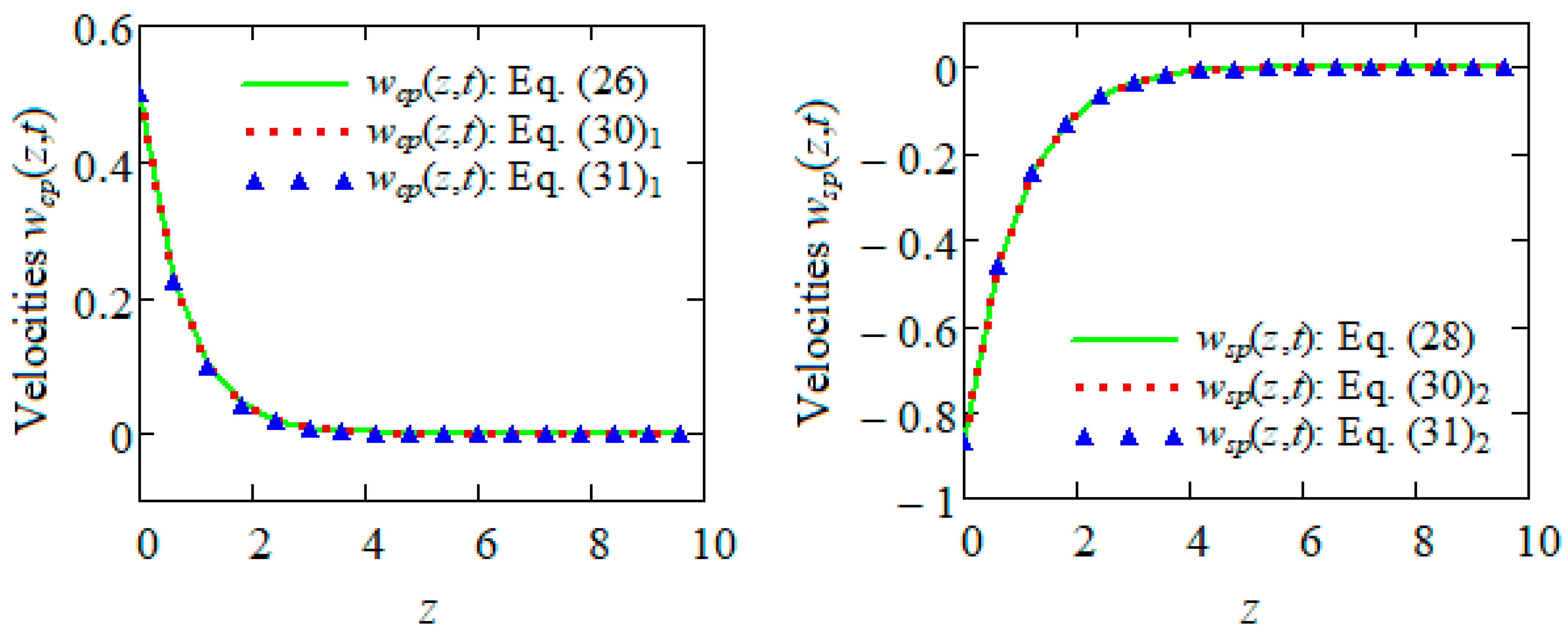
The corresponding expressions for the non-dimensional shear stresses ${\eta }_{cp}(z,t),$ ${\eta }_{ct}(z,t),$ ${\eta }_{sp}(z,t),$ ${\eta }_{st}(z,t)$ and the Darcy’s resistances $R_{cp}(z,t),$ $R_{ct}(z,t),$ $R_{sp}(z,t),$ $R_{st}(z,t)$ can be obtained by substituting $w_{cp}(z,t),$ $w_{ct}(z,t)$ and $w_{sp}(z,t)$, $w_{st}(z,t)$ from Equations (26)–(29) in (11) and (13), respectively. However, since these motions become steady or permanent in time and the required time to reach the steady state is very important for the experimental researchers, we shall present the expressions of their steady state components only but in the simplest forms. In order to do that, we remember the fact that dimensionless steady state components $w_{cp}(z,t),$ $w_{sp}(z,t)$ of $w_c(z,t)$ and $w_s(z,t)$ can be presented in the forms [22]

$$w_{cp}(z,t)={\mathrm{e}}^{-pz}\cos (\omega t-qz), w_{sp}(z,t)={\mathrm{e}}^{-pz}\sin (\omega t-qz); z>0, t\in R,$$

(30)

or equivalently

$$w_{cp}(z,t)=\mathrm{Re}\left\{{\mathrm{e}}^{i\omega t-\delta z}\right\} , w_{sp}(z,t)=\mathrm{Im}\left\{{\mathrm{e}}^{i\omega t-\delta z}\right\}; z>0, t\in R ,$$

(31)

in which

$$\begin{array}{l}p=\sqrt{\frac{\omega }{2}}\hspace{0.17em}\sqrt{\frac{m\omega +\sqrt{{(m\omega )}^2+n^2}}{1+{(\alpha \omega )}^2}},\hspace{0.17em}\hspace{0.17em}\hspace{0.17em}q=\sqrt{\frac{\omega }{2}}\hspace{0.17em}\sqrt{\frac{-m\omega +\sqrt{{(m\omega )}^2+n^2}}{1+{(\alpha \omega )}^2}},\\ m=\alpha +\frac{K_{eff}+{(\alpha \omega )}^{2}K}{{\omega }^2},\hspace{0.17em}\hspace{0.17em}\hspace{0.17em}n=1-\alpha M,\hspace{0.17em}\hspace{0.17em}\hspace{0.17em}\delta =\sqrt{\frac{K_{eff}+i\omega (1+\alpha K)}{1+i\omega \alpha }}.\end{array}$$

Figure 1 clearly shows the equivalence of the expressions of $w_{cp}(z,t)$ and $w_{sp}(z,t)$ given by the Equations (26), (30)₁, (31)₁ and (28), (30)₂, (31)₂, respectively.

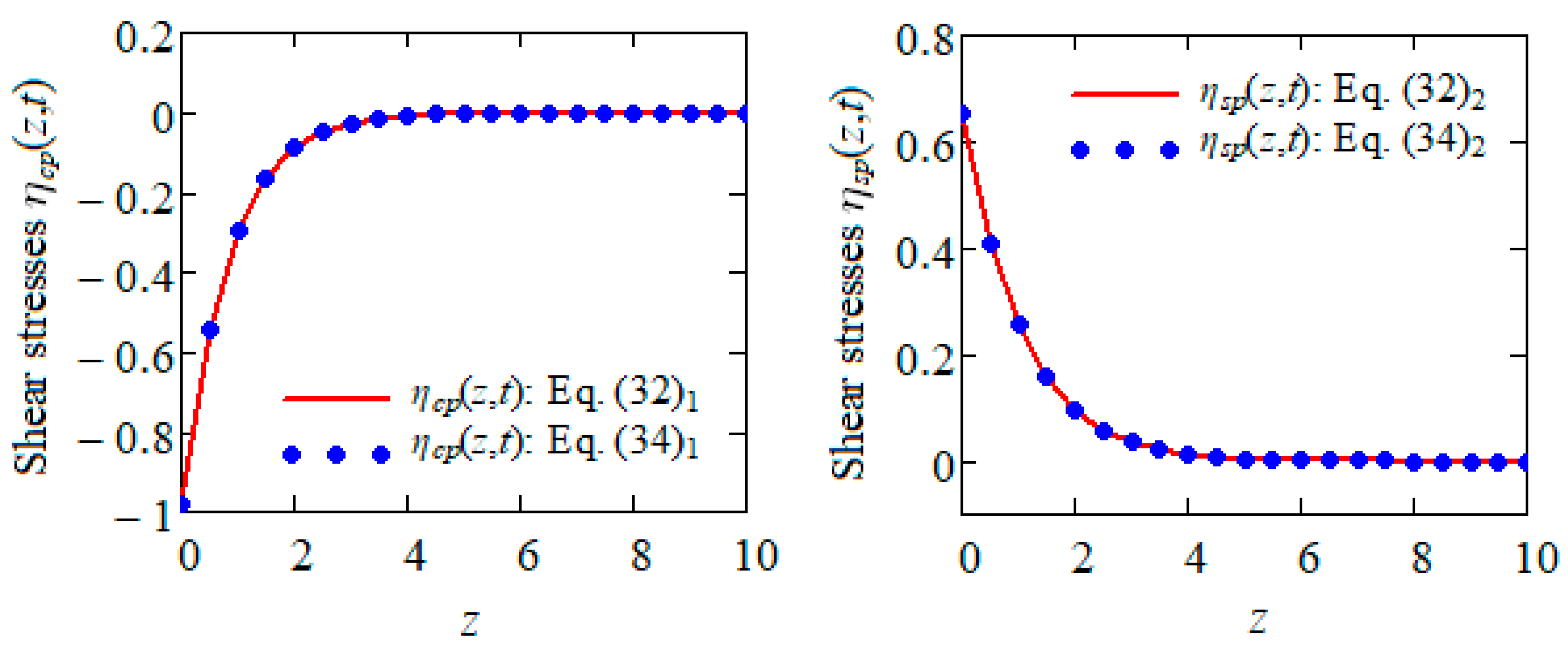
The expressions of the non-dimensional steady state shear stresses ${\eta }_{cp}(z,t),$ ${\eta }_{sp}(z,t)$ and of the Darcy’s resistances $R_{cp}(z,t)$, $R_{sp}(z,t)$ corresponding to the two motions in the discussion also have the simple forms

$${\eta }_{cp}(z,t)=-r{\mathrm{e}}^{-pz}\cos (\omega t-qz-\phi ), {\eta }_{sp}(z,t)=-r{\mathrm{e}}^{-pz}\sin (\omega t-qz-\phi ); z>0, t\in R,$$

(32)

$$\begin{array}{l}{R}_{cp}(z,t)=-K\sqrt{1+{(\alpha \omega )}^2}{\mathrm{e}}^{-pz}\cos (\omega t-qz+\psi );\hspace{0.17em}\hspace{0.17em}z>0,\hspace{0.17em}\hspace{0.17em}t\in R,\\ R_{sp}(z,t)=-K\sqrt{1+{(\alpha \omega )}^2}{\mathrm{e}}^{-pz}\sin (\omega t-qz+\psi );\hspace{0.17em}\hspace{0.17em}z>0,\hspace{0.17em}\hspace{0.17em}t\in R,\end{array}$$

(33)

or equivalent

$${\eta }_{cp}(z,t)=-\mathrm{Re}\{(1+i\omega \alpha )\delta {\mathrm{e}}^{i\omega t-\delta z}\} , {\eta }_{sp}(z,t)=-\mathrm{Im}\{(1+i\omega \alpha )\delta {\mathrm{e}}^{i\omega t-\delta z}\} ; z>0, t\in R,\hspace{0.17em}$$

(34)

$$R_{cp}(z,t)=-K\mathrm{Re}\{(1+i\omega \alpha ){\mathrm{e}}^{i\omega t-\delta z}\} , R_{sp}(z,t)=-K\mathrm{Im}\{(1+i\omega \alpha ){\mathrm{e}}^{i\omega t-\delta z}\} ; z>0, t\in R,\hspace{0.17em}$$

(35)

where

$$r=\sqrt{{(\alpha \omega p+q)}^2+{(\alpha \omega q-p)}^2}, \phi =\mathrm{arctg}\left(\frac{\alpha \omega p+q}{\alpha \omega q-p}\right), \psi =\mathrm{arctg}(\alpha \omega ).$$

Figure 2 shows the equivalence of the expressions of ${\eta }_{cp}(z,t)$ and ${\eta }_{sp}(z,t)$ given by the Equations (32)₁, (34)₁ and (32)₂, (34)₂, respectively. The equivalence of the expressions of the corresponding Darcy’s resistances $R_{cp}(z,t)$ and $R_{sp}(z,t)$ given by Equations (33)₁, (35)₁ and (33)₂, (35)₂, respectively, has been proved in the reference [22].

In all cases, the solutions corresponding to incompressible Newtonian fluids performing the same motions are immediately obtained, taking $\alpha =0$ in the above relations. In addition, if we want to eliminate the magnetic or porous effects, it is sufficient to put $M=0$ or $K=0$, respectively, in the previous solutions. In the absence of both effects, for instance, the dimensionless starting velocity fields $w_c(z,t)$ and $w_s(z,t)$ have the simplified forms

$$\begin{array}{l}{w}_c(z,t)=\cos (\omega t)-\frac{2{\omega }^2\cos (\omega t)}{\pi }{\displaystyle \underset{0}{\overset{\infty }{\int }}\frac{(1+\alpha {\xi }^2)\sin (z\xi )}{\xi [{\xi }^4+{\omega }^2{(1+\alpha {\xi }^2)}^2]}}d\xi \\ +\frac{2\omega \sin (\omega t)}{\pi }{\displaystyle \underset{0}{\overset{\infty }{\int }}\frac{\xi \sin (z\xi )}{{\xi }^4+{\omega }^2{(1+\alpha {\xi }^2)}^2}}d\xi \\ -\frac{2}{\pi }{\displaystyle \underset{0}{\overset{\infty }{\int }}\frac{{\xi }^3\sin (z\xi )}{{\xi }^4+{\omega }^2{(1+\alpha {\xi }^2)}^2}\exp \left(-\frac{{\xi }^{2}t}{1+\alpha {\xi }^2}\right)d\xi ;\hspace{0.17em}\hspace{0.17em}z>0,\hspace{0.17em}\hspace{0.17em}t>0},\end{array}$$

(36)

$$\begin{array}{l}{w}_s(z,t)=\sin (\omega t)-\frac{2{\omega }^2\sin (\omega t)}{\pi }{\displaystyle \underset{0}{\overset{\infty }{\int }}\frac{(1+\alpha {\xi }^2)\sin (z\xi )}{\xi [{\xi }^4+{\omega }^2{(1+\alpha {\xi }^2)}^2]}}d\xi \\ -\frac{2\omega \cos (\omega t)}{\pi }{\displaystyle \underset{0}{\overset{\infty }{\int }}\frac{\xi \sin (z\xi )}{{\xi }^4+{\omega }^2{(1+\alpha {\xi }^2)}^2}}d\xi \\ +\frac{2\omega }{\pi }{\displaystyle \underset{0}{\overset{\infty }{\int }}\frac{\xi \sin (z\xi )}{{\xi }^4+{\omega }^2{(1+\alpha {\xi }^2)}^2}\exp \left(-\frac{{\xi }^{2}t}{1+\alpha {\xi }^2}\right)d\xi ;\hspace{0.17em}\hspace{0.17em}z>0,\hspace{0.17em}\hspace{0.17em}t>0}.\end{array}$$

(37)

3.2. The First Problem of Stokes

Making $\omega =0$ in Equation (25)₁, in which $w_{cp}(z,t)$ and $w_{ct}(z,t)$ are given by Equations (26) and (27), respectively, one finds the dimensionless velocity field

$$\begin{array}{l}{w}_C(z,t)=1-\frac{2K_{eff}}{\pi }{\displaystyle \underset{0}{\overset{\infty }{\int }}\frac{\sin (z\xi )}{\xi ({\xi }^2+K_{eff})}}d\xi \\ +\frac{2(\alpha M-1)}{\pi }{\displaystyle \underset{0}{\overset{\infty }{\int }}\frac{\xi \sin (z\xi )}{({\xi }^2+K_{eff})[1+\alpha ({\xi }^2+K)]}\exp \left(-\frac{{\xi }^2+K_{eff}}{1+\alpha ({\xi }^2+K)}t\right)d\xi };\hspace{0.17em}\hspace{0.17em}z>0,\hspace{0.17em}\hspace{0.17em}t>0,\end{array}$$

(38)

corresponding to the MHD motion of the same fluids over an infinite flat plate which, after the moment $t=0^{+}$, slides in its plane with the constant velocity W through a porous medium. This motion is known in the literature as “the first problem of Stokes”.

Expressions of the dimensionless shear stress ${\eta }_C(z,t)$ and the Darcy’s resistance $R_C(z,t)$ corresponding to the first problem of Stokes, namely

$$\begin{array}{l}{\eta }_C(z,t)=-\frac{2K_{eff}}{\pi }{\displaystyle \underset{0}{\overset{\infty }{\int }}\frac{\cos (z\xi )}{{\xi }^2+K_{eff}}}d\xi -\frac{2{(\alpha M-1)}^2}{\pi }\\ \times {\displaystyle \underset{0}{\overset{\infty }{\int }}\frac{{\xi }^2\cos (z\xi )}{({\xi }^2+K_{eff}){[1+\alpha ({\xi }^2+K)]}^2}}\exp \left[-\frac{{\xi }^2+K_{eff}}{1+\alpha ({\xi }^2+K)}t\right]d\xi ;\hspace{0.17em}\hspace{0.17em}z>0,\hspace{0.17em}\hspace{0.17em}t>0\hspace{0.17em},\end{array}$$

(39)

$$\begin{array}{l}{R}_C(z,t)=-K\left[1-\frac{2K_{eff}}{\pi }{\displaystyle \underset{0}{\overset{\infty }{\int }}\frac{\sin (z\xi )}{\xi ({\xi }^2+K_{eff})}}d\xi \right]\\ -\frac{2K{(\alpha M-1)}^2}{\pi }{\displaystyle \underset{0}{\overset{\infty }{\int }}\frac{\xi \sin (z\xi )}{({\xi }^2+K_{eff}){[1+\alpha ({\xi }^2+K)]}^2}}\exp \left[-\frac{{\xi }^2+K_{eff}}{1+\alpha ({\xi }^2+K)}t\right]d\xi ;\hspace{0.17em}\hspace{0.17em}z>0,\hspace{0.17em}\hspace{0.17em}t>0,\end{array}$$

(40)

have been obtained by introducing $w_C(z,t)$ from Equation (38) in (11) and (13). The corresponding Newtonian solutions $w_{NC}(z,t),$ ${\eta }_{NC}(z,t),$ $R_{NC}(z,t)$ can be immediately obtained, making $\alpha =0$ in Equations (38)–(40), respectively.

The steady components $w_{Cp}(z),$ ${\eta }_{Cp}(z)$ and $R_{Cp}(z)$ of the starting solutions $w_C(z,t)$, ${\eta }_C(z,t)$ and $R_C(z,t)$, respectively, are given by the next relations

$$\begin{array}{l}{w}_{Cp}(z)=1-\frac{2K_{eff}}{\pi }{\displaystyle \underset{0}{\overset{\infty }{\int }}\frac{\sin (z\xi )}{\xi ({\xi }^2+K_{eff})}}d\xi ,\hspace{0.17em}\hspace{0.17em}\hspace{0.17em}{\eta }_{Cp}(z)=-\frac{2K_{eff}}{\pi }{\displaystyle \underset{0}{\overset{\infty }{\int }}\frac{\cos (z\xi )}{{\xi }^2+K_{eff}}}d\xi ,\\ R_{Cp}(z)=-K\left[1-\frac{2K_{eff}}{\pi }{\displaystyle \underset{0}{\overset{\infty }{\int }}\frac{\sin (z\xi )}{\xi ({\xi }^2+K_{eff})}}d\xi \right]\hspace{0.17em};\hspace{0.17em}\hspace{0.17em}z>0,\hspace{0.17em}\hspace{0.17em}t\in R\hspace{0.17em}.\end{array}$$

(41)

As expected, they are the same both for second grade and Newtonian fluids. Using entries 2 and 3 of Tables 4 and 5, respectively, of the reference [26], the result is that these solutions can be written in the simple forms

$$w_{Cp}(z)={\mathrm{e}}^{-z\sqrt{K_{eff}}}, {\eta }_{Cp}(z)=-\sqrt{K_{eff}}{\mathrm{e}}^{-z\sqrt{K_{eff}}}, R_{Cp}(z)=-K{\mathrm{e}}^{-z\sqrt{K_{eff}}}; z>0, t\in R.$$

(42)

In the absence of magnetic and porous effects, $R_C(z,t)=0$ and

$$w_C(z,t)=1-\frac{2}{\pi }{\displaystyle \underset{0}{\overset{\infty }{\int }}\frac{\sin (z\xi )}{\xi (1+\alpha {\xi }^2)}\exp \left(-\frac{{\xi }^{2}t}{1+\alpha {\xi }^2}\right)d\xi }; z>0, t>0,$$

(43)

$${\eta }_C(z,t)=-\frac{2}{\pi }{\displaystyle \underset{0}{\overset{\infty }{\int }}\frac{\cos (z\xi )}{{(1+\alpha {\xi }^2)}^2}}\exp \left[-\frac{{\xi }^{2}t}{1+\alpha {\xi }^2}\right]d\xi ; z>0, t>0.$$

(44)

The velocity field $w_C(z,t)$ given by Equation (43) has been obtained by Christov [27]. Taking $\alpha =0$ in Equations (43) and (44) and using entries 5 and 1 of Tables 4 and 5, respectively, from the reference [26], the classical solutions corresponding to the first problem of Stokes for incompressible Newtonian fluids, namely

$$w_{classic}(z,t)=\mathrm{Erfc}\left(\frac{z}{2\sqrt{t}}\right), {\eta }_{classic}(z,t)=-\frac{1}{\sqrt{\pi t}}\exp \left(-\frac{z^2}{4t}\right) ; z>0, t>0,$$

(45)

are immediately recovered.

4. Motion Due to the Plate That Applies a Shear Stress Sg(t) to the Fluid

As already seen in Section 2, the velocity vector and governing equations corresponding to this motion are characterized by the same Equations (3)–(6). The initial conditions are also given by Equation (9), while the boundary conditions are given by Equation (8). Introducing the following non-dimensional functions, variables and parameter

$$\begin{array}{l}{w}^{\ast }=w\sqrt{\frac{\rho }{S}}, {\eta }^{\ast }=\frac{1}{S}\eta , R^{\ast }=\frac{\nu \sqrt{\rho }}{S\sqrt{S}}R, z^{\ast }=\frac{z}{\nu }\sqrt{\frac{S}{\rho }}, \\ t^{\ast }=\frac{S}{\mu }t, {\alpha }^{\ast }=\frac{\alpha S}{{\mu }^2}, g^{\ast }(z^{\ast },t^{\ast })=g\left(\nu z^{\ast }\sqrt{\frac{\rho }{S}},\frac{\mu }{S}{t}^{\ast }\right)\end{array}$$

(46)

and again dropping out the star notation, dimensionless governing equations corresponding to this motion have identical forms to those from relations (11)–(13) in which

$$M=\frac{\sigma B^2}{\rho }\frac{\mu }{S}=\frac{\nu }{S}\sigma B^2, K=\frac{\phi }{k}\frac{\mu \nu }{S}.$$

(47)

Dimensionless initial and boundary conditions corresponding to this problem are

$$w(z,0)=0, \eta (z,0)=0; z\ge 0,$$

(48)

respectively,

$$\eta (0,t)=g(t), \underset{z\to \infty }{\lim } \eta (z,t)=0, \underset{z\to \infty }{\lim } w(z,t)=0; t>0.$$

(49)

Eliminating the velocity $w(z,t)$ between Equations (11) and (12) and having Equation (13) in mind, one finds the following partial differential equation

$$\frac{\partial \eta (z,t)}{\partial t}=\left(1+\alpha \frac{\partial }{\partial t}\right)\frac{{\partial }^2\eta (z,t)}{\partial z^2}-M\eta (z,t)-K\left(1+\alpha \frac{\partial }{\partial t}\right)\eta (z,t); z>0, t>0,$$

(50)

for the dimensionless shear stress $\eta (z,t)$.

The governing Equation (50) is identical in form to the governing Equation (15) of the dimensionless velocity field $w(z,t)$. Consequently, bearing in mind the corresponding initial and boundary conditions as well as the expression of $w(z,t)$ from the previous section, the result is that

$$\begin{array}{l}\eta (z,t)=g(t)-\frac{2K_{eff}g(t)}{\pi }{\displaystyle \underset{0}{\overset{\infty }{\int }}\frac{\sin (z\xi )}{\xi ({\xi }^2+K_{eff})}}d\xi +\frac{2(\alpha M-1)}{\pi }{\displaystyle \underset{0}{\overset{\infty }{\int }}\frac{\xi \sin (z\xi )}{({\xi }^2+K_{eff})[1+\alpha ({\xi }^2+K)]}}\\ \times {\displaystyle \underset{0}{\overset{t}{\int }}{g}^{\prime }(s)}\hspace{0.17em}\exp \left[-\frac{{\xi }^2+K_{eff}}{1+\alpha ({\xi }^2+K)}(t-s)\right]dsd\xi ; z>0, t>0.\end{array}$$

(51)

Once the dimensionless shear stress $\eta (z,t)$ is known for a given function $g(\cdot )$, the corresponding velocity field $w(z,t)$ can be immediately determined by solving the linear ordinary differential Equation (12), in which $R(z,t)$ is given by Equation (13). The Darcy’s resistance $R(z,t)$ is then obtained using Equation (13). For exemplification, we consider two special cases when the flat plate applies oscillatory shear stresses or constant shear stress to the fluid.

4.1. The Case $g(t)$ Equal to $H(t)\cos (\omega t)$ or $H(t)\sin (\omega t)$

Bearing in mind the previous results, the result is that the dimensionless starting shear stresses ${\eta }_c(z,t)$, ${\eta }_s(z,t)$ corresponding to this motion can be written in the forms

$${\eta }_c(z,t)={\eta }_{cp}(z,t)+{\eta }_{ct}(z,t), {\eta }_s(z,t)={\eta }_{sp}(z,t)+{\eta }_{st}(z,t); z>0, t>0,$$

(52)

where

$$\begin{array}{l}{\eta }_{cp}(z,t)=\cos (\omega t)\\ -\frac{2\cos (\omega t)}{\pi }{\displaystyle \underset{0}{\overset{\infty }{\int }}\frac{K_{eff}({\xi }^2+K_{eff})+{\omega }^2(\alpha K+1)[1+\alpha ({\xi }^2+K)]}{{({\xi }^2+K_{eff})}^2+{\omega }^2{[1+\alpha ({\xi }^2+K)]}^2}\frac{\sin (z\xi )}{\xi }}d\xi \\ +\frac{2\omega (1-\alpha M)\sin (\omega t)}{\pi }{\displaystyle \underset{0}{\overset{\infty }{\int }}\frac{\xi \sin (z\xi )}{{({\xi }^2+K_{eff})}^2+{\omega }^2{[1+\alpha ({\xi }^2+K)]}^2}}d\xi ,\end{array}$$

(53)

$$\begin{array}{l}{\eta }_{ct}(z,t)=\frac{2(\alpha M-1)}{\pi }{\displaystyle \underset{0}{\overset{\infty }{\int }}\frac{\xi ({\xi }^2+K_{eff})\sin (z\xi )}{\{{({\xi }^2+K_{eff})}^2+{\omega }^2{[1+\alpha ({\xi }^2+K)]}^2\}[1+\alpha ({\xi }^2+K)]}}\\ \times \exp \left[-\frac{{\xi }^2+K_{eff}}{1+\alpha ({\xi }^2+K)}t\right]d\xi ,\end{array}$$

(54)

$$\begin{array}{l}{\eta }_{sp}(z,t)=\sin (\omega t)\\ -\frac{2\sin (\omega t)}{\pi }{\displaystyle \underset{0}{\overset{\infty }{\int }}\frac{K_{eff}({\xi }^2+K_{eff})+{\omega }^2(\alpha K+1)[1+\alpha ({\xi }^2+K)]}{{({\xi }^2+K_{eff})}^2+{\omega }^2{[1+\alpha ({\xi }^2+K)]}^2}\frac{\sin (z\xi )}{\xi }}d\xi \\ +\frac{2\omega (\alpha M-1)}{\pi }\cos (\omega t){\displaystyle \underset{0}{\overset{\infty }{\int }}\frac{\xi \sin (z\xi )}{{({\xi }^2+K_{eff})}^2+{\omega }^2{[1+\alpha ({\xi }^2+K)]}^2}}d\xi ,\end{array}$$

(55)

$$\begin{array}{l}{\eta }_{st}(z,t)=\frac{2\omega (1-\alpha M)}{\pi }{\displaystyle \underset{0}{\overset{\infty }{\int }}\frac{\xi \sin (z\xi )}{{({\xi }^2+K_{eff})}^2+{\omega }^2{[1+\alpha ({\xi }^2+K)]}^2}}\\ \times \exp \left[-\frac{{\xi }^2+K_{eff}}{1+\alpha ({\xi }^2+K)}t\right]d\xi ,\end{array}$$

(56)

In addition, the dimensionless steady state components ${\eta }_{cp}(z,t)$ and ${\eta }_{sp}(z,t)$ can also be written in equivalent forms, i.e.,

$${\eta }_{cp}(z,t)={\mathrm{e}}^{-pz}\cos (\omega t-qz), {\eta }_{sp}(z,t)={\mathrm{e}}^{-pz}\sin (\omega t-qz); z>0, t\in R,$$

(57)

or

$${\eta }_{cp}(z,t)=\mathrm{Re}\left\{{\mathrm{e}}^{i\omega t-\delta z}\right\} , {\eta }_{sp}(z,t)=\mathrm{Im}\left\{{\mathrm{e}}^{i\omega t-\delta z}\right\}; z>0, t\in R ,$$

(58)

in which the constants p, q and $\delta$ have the same significations as in the previous section.

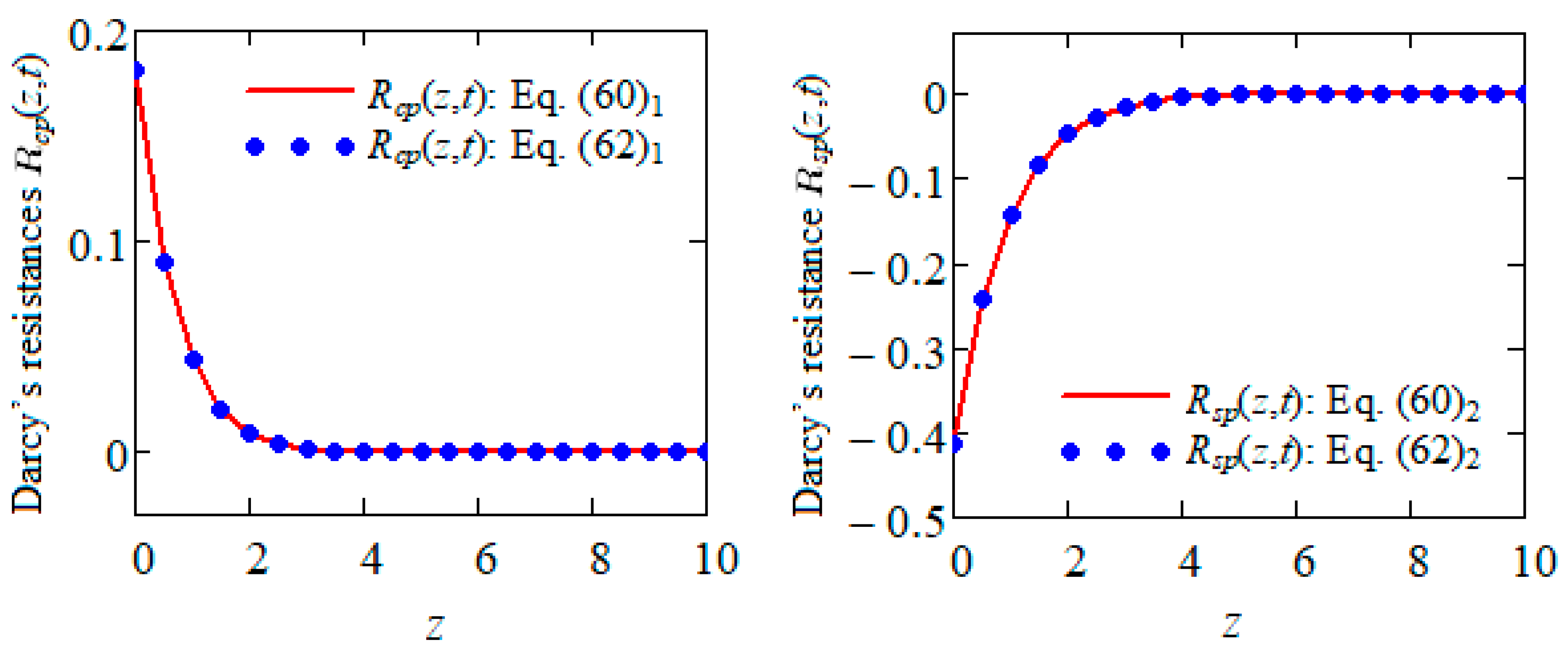
Lengthy but straightforward computations show that dimensionless steady state velocities $w_{cp}(z,t)$, $w_{sp}(z,t)$ and the Darcy’s resistances $R_{cp}(z,t)$, $R_{sp}(z,t)$ corresponding to these two motions are given by the following relations:

$$\begin{array}{l}{w}_{cp}(z,t)=\frac{1}{r}{\mathrm{e}}^{-pz}\cos (\omega t-qz+\phi ),\\ w_{sp}(z,t)=\frac{1}{r}{\mathrm{e}}^{-pz}\sin (\omega t-qz+\phi );\hspace{0.17em}\hspace{0.17em}z>0,\hspace{0.17em}\hspace{0.17em}t\in R,\end{array}$$

(59)

$$\begin{array}{l}{R}_{cp}(z,t)=\frac{K}{r}\sqrt{1+{(\alpha \omega )}^2}{\mathrm{e}}^{-pz}\cos (\omega t-qz+\phi +\psi );\hspace{0.17em}\hspace{0.17em}z>0,\hspace{0.17em}\hspace{0.17em}t\in R,\\ R_{sp}(z,t)=\frac{K}{r}\sqrt{1+{(\alpha \omega )}^2}{\mathrm{e}}^{-pz}\sin (\omega t-qz+\phi +\psi );\hspace{0.17em}\hspace{0.17em}z>0,\hspace{0.17em}\hspace{0.17em}t\in R,\end{array}$$

(60)

or equivalently

$$\begin{array}{l}{w}_{cp}(z,t)=-\mathrm{Re}\left\{\frac{1}{\delta (1+i\omega \alpha )}{\mathrm{e}}^{i\omega t-\delta z}\right\} ,\hspace{0.17em}\hspace{0.17em}\\ w_{sp}(z,t)=-\mathrm{Im}\left\{\frac{1}{\delta (1+i\omega \alpha )} {\mathrm{e}}^{i\omega t-\delta z}\right\};\hspace{0.17em}\hspace{0.17em}z>0,\hspace{0.17em}\hspace{0.17em}t\in R ,\hspace{0.17em}\end{array}$$

(61)

$$R_{cp}(z,t)=K\mathrm{Re}\left\{\frac{1}{\delta }{\mathrm{e}}^{i\omega t-\delta z}\right\}, R_{sp}(z,t)=K\mathrm{Im}\left\{\frac{1}{\delta }{\mathrm{e}}^{i\omega t-\delta z}\right\}; z>0, t\in R ,\hspace{0.17em}$$

(62)

The equivalence of the expressions of Darcy’s resistances $R_{cp}(z,t)$ and $R_{sp}(z,t)$ given by the relations (60)₁, (62)₁ and (60)₂, (62)₂, respectively, is proved by Figure 3.

As a check of the results’ correctness, here, we include

Table 1. Values of Darcy’s resistances given by Equations (60) and (62).

y	${\mathit{R}}_{\mathit{c}\mathit{p}}(\mathit{z})$ $\mathbf{Given} \mathbf{by} \mathbf{Equation} {(60)}_1$	${\mathit{R}}_{\mathit{c}\mathit{p}}(\mathit{z})$ $\mathbf{Given} \mathbf{by} \mathbf{Equation} {(62)}_1$	${\mathit{R}}_{\mathit{s}\mathit{p}}(\mathit{z})$ $\mathbf{Given} \mathbf{by} \mathbf{Equation} {(60)}_2$	${\mathit{R}}_{\mathit{s}\mathit{p}}(\mathit{z})$ $\mathbf{Given} \mathbf{by} \mathbf{Equation} {(62)}_2$
0	$0.181$	$0.181$	$-0.413$	$-0.413$
0.5	$0.090$	$0.090$	$-0.244$	$-0.244$
1.0	$0.043$	$0.043$	$-0.144$	$-0.144$
1.5	$0.020$	$0.020$	$-0.084$	$-0.084$
2.0	$8.466\cdot {10}^{-3}$	$8.466\cdot {10}^{-3}$	$-0.049$	$-0.049$
2.5	$3.151\cdot {10}^{-3}$	$3.151\cdot {10}^{-3}$	$-0.029$	$-0.029$
3.0	$8.127\cdot {10}^{-4}$	$8.127\cdot {10}^{-4}$	$-0.017$	$-0.017$
3.5	$-1.122\cdot {10}^{-4}$	$-1.122\cdot {10}^{-4}$	$-9.558\cdot {10}^{-3}$	$-9.558\cdot {10}^{-3}$
4.0	$-3.993\cdot {10}^{-4}$	$-3.993\cdot {10}^{-4}$	$-5.497\cdot {10}^{-3}$	$-5.497\cdot {10}^{-3}$
4.5	$-4.223\cdot {10}^{-4}$	$-4.223\cdot {10}^{-4}$	$-3.149\cdot {10}^{-3}$	$-3.149\cdot {10}^{-3}$
5.0	$-3.533\cdot {10}^{-4}$	$-3.533\cdot {10}^{-4}$	$-1.798\cdot {10}^{-3}$	$-1.798\cdot {10}^{-3}$
5.5	$-2.663\cdot {10}^{-4}$	$-2.663\cdot {10}^{-4}$	$-1.022\cdot {10}^{-3}$	$-1.022\cdot {10}^{-3}$
6.0	$-1.890\cdot {10}^{-4}$	$-1.890\cdot {10}^{-4}$	$-5.790\cdot {10}^{-4}$	$-5.790\cdot {10}^{-4}$
6.5	$-1.291\cdot {10}^{-4}$	$-1.291\cdot {10}^{-4}$	$-3.266\cdot {10}^{-4}$	$-3.266\cdot {10}^{-4}$
7.0	$-8.572\cdot {10}^{-5}$	$-8.572\cdot {10}^{-5}$	$-1.834\cdot {10}^{-4}$	$-1.834\cdot {10}^{-4}$
7.5	$-5.575\cdot {10}^{-5}$	$-5.575\cdot {10}^{-5}$	$-1.026\cdot {10}^{-4}$	$-1.026\cdot {10}^{-4}$
8.0	$-3.568\cdot {10}^{-5}$	$-3.568\cdot {10}^{-5}$	$-5.707\cdot {10}^{-5}$	$-5.707\cdot {10}^{-5}$
8.5	$-2.253\cdot {10}^{-5}$	$-2.253\cdot {10}^{-5}$	$-3.160\cdot {10}^{-5}$	$-3.160\cdot {10}^{-5}$
9.0	$-1.407\cdot {10}^{-5}$	$-1.407\cdot {10}^{-5}$	$-1.739\cdot {10}^{-5}$	$-1.739\cdot {10}^{-5}$
9.5	$-8.709\cdot {10}^{-6}$	$-8.709\cdot {10}^{-6}$	$-9.518\cdot {10}^{-6}$	$-9.518\cdot {10}^{-6}$
10	$-5.345\cdot {10}^{-6}$	$-5.345\cdot {10}^{-6}$	$-5.173\cdot {10}^{-6}$	$-5.173\cdot {10}^{-6}$

for the values of Darcy’s resistances $R_{cp}(z,t)$ and $R_{sp}(z,t)$, which are given by the Equations (60) and (62).

These values correspond to $t=10, \alpha =0.7, \omega =\pi /6,$ $M=0.6$ and $K=0.5$.

4.2. The Case $g(t)$ Equal to $H(t)$

Making $\omega =0$ in Equation (52)₁, in which ${\eta }_{cp}(z,t)$ and ${\eta }_{ct}(z,t)$ are given by Equations (53) and (54), one finds the dimensionless shear stress

$$\begin{array}{l}{\eta }_S(z,t)=1-\frac{2K_{eff}}{\pi }{\displaystyle \underset{0}{\overset{\infty }{\int }}\frac{\sin (z\xi )}{\xi ({\xi }^2+K_{eff})}}d\xi \\ +\frac{2(\alpha M-1)}{\pi }{\displaystyle \underset{0}{\overset{\infty }{\int }}\frac{\xi \sin (z\xi )}{({\xi }^2+K_{eff})[1+\alpha ({\xi }^2+K)]}\exp \left(-\frac{{\xi }^2+K_{eff}}{1+\alpha ({\xi }^2+K)}t\right)d\xi };\hspace{0.17em}\hspace{0.17em}z>0,\hspace{0.17em}\hspace{0.17em}t>0,\end{array}$$

(63)

corresponding to the motion of incompressible second grade fluid induced by the lower plate that applies a constant shear stress S to the fluid after the moment $t=0^{+}$. Direct computations show that the steady solutions $w_{Sp}(z)$, ${\eta }_{Sp}(z)$ and $R_{Sp}(z)$ corresponding to this motion have the simple expressions

$$w_{Sp}(z)=-\frac{1}{\sqrt{K_{eff}}}{\mathrm{e}}^{-z\sqrt{K_{eff}}}, {\eta }_{Sp}(z)={\mathrm{e}}^{-z\sqrt{K_{eff}}}, R_{Sp}(z)=\frac{K}{\sqrt{K_{eff}}}{\mathrm{e}}^{-z\sqrt{K_{eff}}}; z>0, t\in R,$$

(64)

which are the same for both incompressible second grade and Newtonian fluids.

5. Influence of Magnetic Field and Porous Medium on Steady State and the Flow Resistance of Fluid

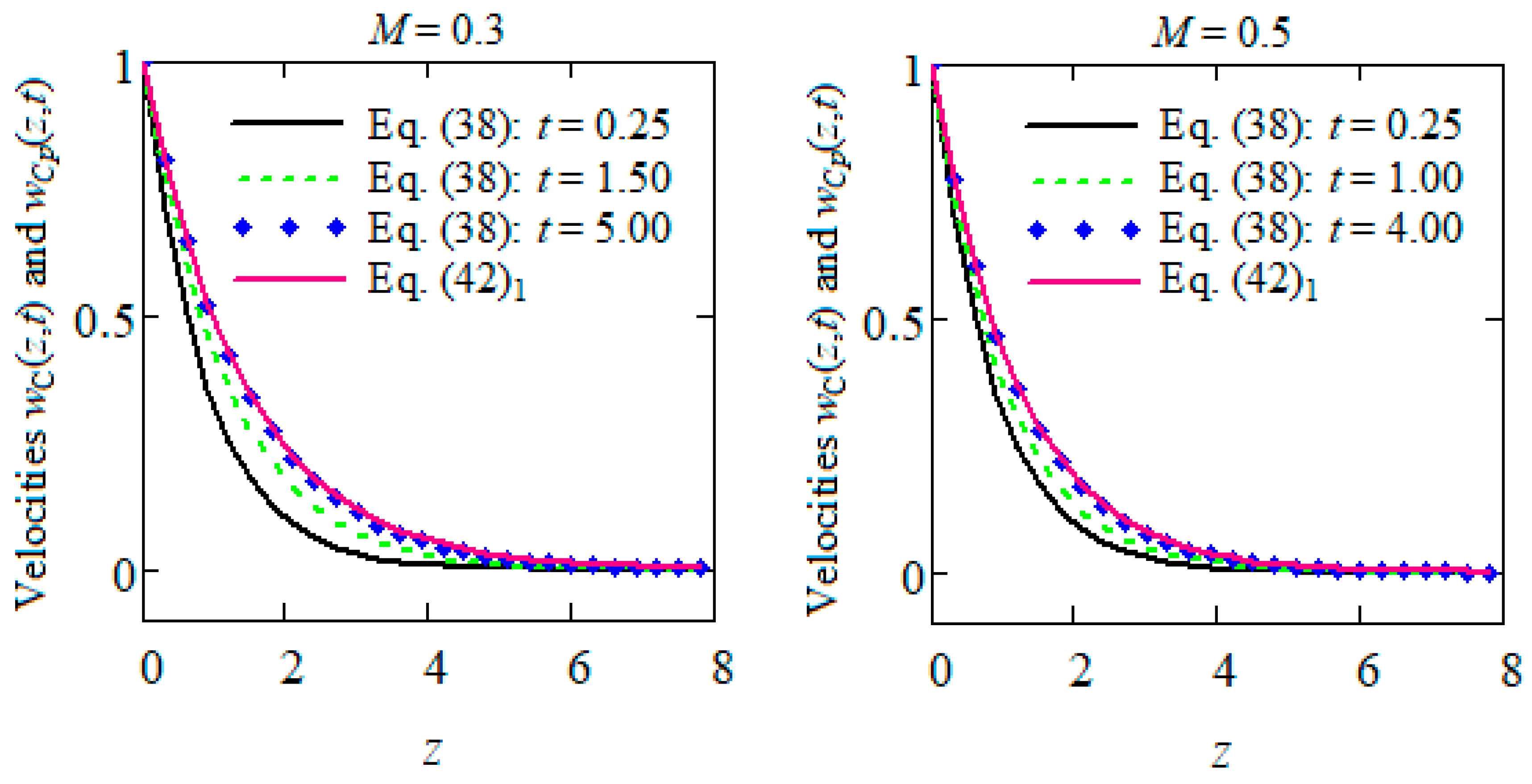
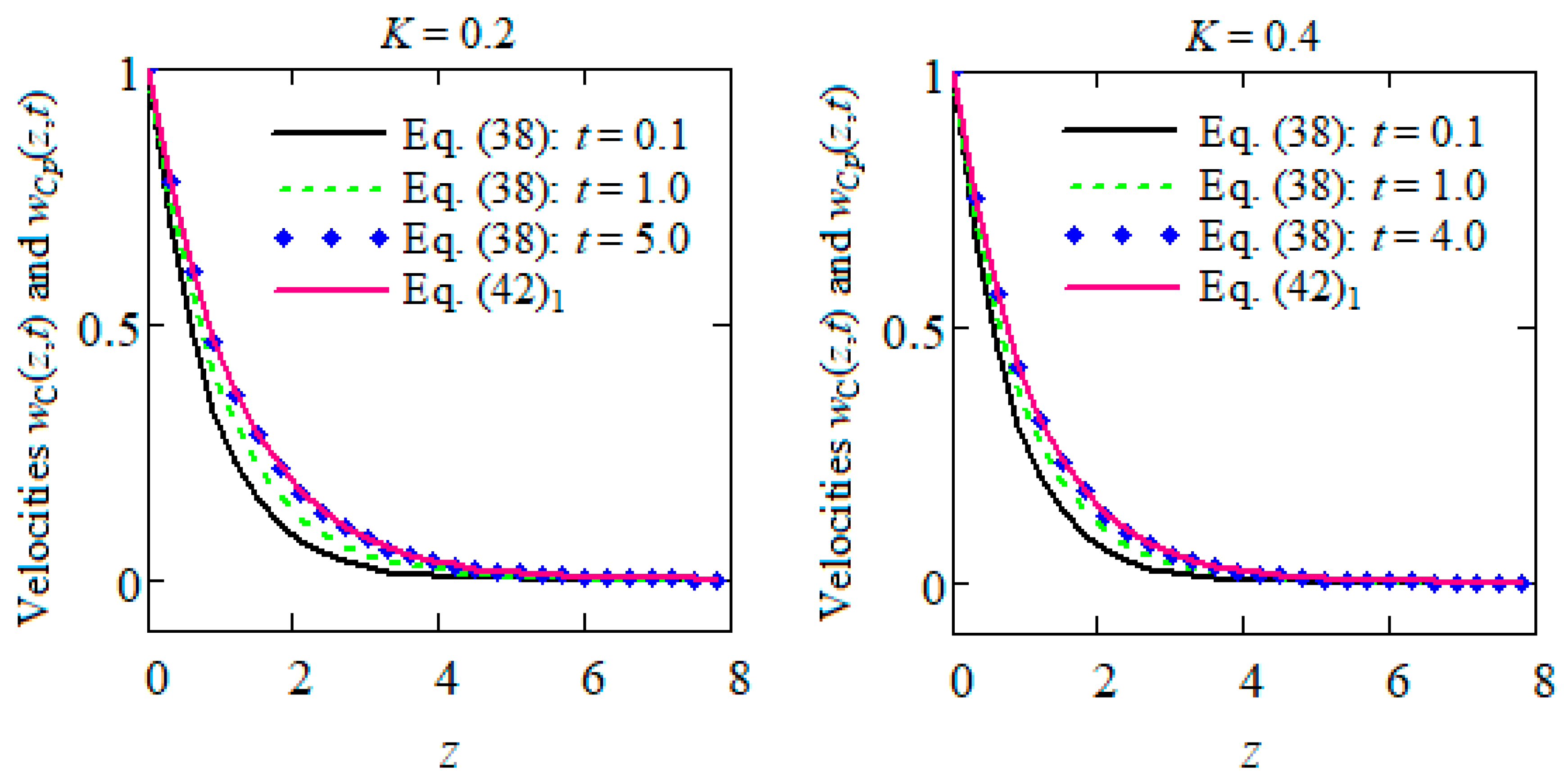
All exact solutions that have been previously determined correspond to isothermal unsteady motions, which become steady over time. The corresponding starting solutions describe the fluid motion sometime after its initiation. After this time, the fluid behavior can be characterized by the corresponding steady state solutions, which satisfy governing equations and boundary conditions but are independent of the initial conditions. From a mathematical point of view, it is the time after which the diagrams of starting solutions overlap with those of the steady state solutions (steady state components of starting solutions). This time is very important for experimental researchers who want to know the transition moment of the motion toward the steady state. From Figure 4 and Figure 5, which show the convergence of the starting solution $w_C(z,t)$ given by Equation (38) to its steady component $w_{Cp}(z)$ (from Equation (41)₁ or (42)₁) for increasing values of the dimensionless time t and distinct values of M and K, the result is that the steady state for the first problem of Stokes of incompressible second grade fluids is earlier obtained in the presence of a magnetic field or porous medium.

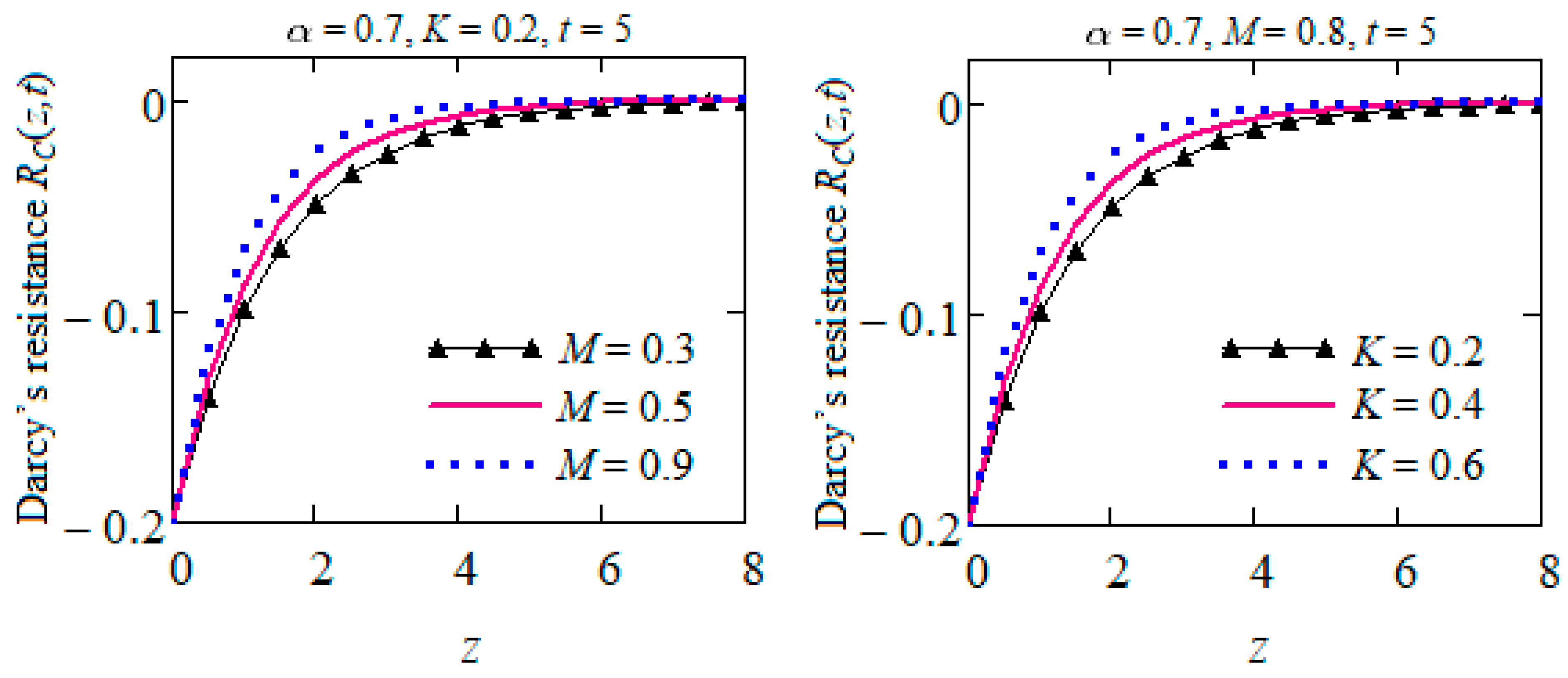
In order to show the flow resistance of the fluid, the variations of the Darcy’s resistance $R_C(z,t)$ against z given by Equation (40) are presented in Figure 6 for $\alpha =0.7, K=\hspace{0.17em}0.2, t=5$ and increasing values of the magnetic parameter M and $\alpha =\hspace{0.17em}0.7, M=0.8, t=\hspace{0.17em}5$ and increasing values of the porosity parameter K. From these figures, the result is clearly that the flow resistance of fluid, in absolute value, declines for increasing values of M and is an increasing function with respect to the parameter K. Consequently, the fluid flows faster in the presence of a magnetic field while its velocity, as expected, diminishes through porous media.

6. Conclusions

In the present work, the first exact general solutions for isothermal MHD motions of the incompressible second grade fluids over an infinite flat plate incorporated in a porous medium are determined. The fluid motion is induced by the flat plate that, after the moment $t=0^{+}$, begins to move in its plane with the time-dependent velocity $Wf(t)$. Closed-form expressions are established for the dimensionless velocity field $w(z,t)$, the corresponding non-trivial shear stress $\eta (z,t)$ and the Darcy’s resistance $R(z,t)$. For illustration, as well as for the validation of the obtained results, some motions with engineering applications are considered, and the steady state components $w_{cp}(z,t)$, $w_{sp}(z,t)$ of the dimensionless starting velocities $w_c(z,t)$, $w_s(z,t)$ are presented in three different forms whose equivalence was graphically proved in Figure 1. The equivalence of the expressions of the dimensionless steady state shear stresses ${\eta }_{cp}(z,t)$ and ${\eta }_{sp}(z,t)$ given by Equations (32)₁, (34)₁ and (32)₂, (34)₂, respectively, was proved by Figure 2.

In the next section, based on an important remark regarding the governing equations of velocity and shear stress for such motions of incompressible second grade fluids, a general expression for the dimensionless starting shear stress corresponding to the motion produced by the flat plate that applies a time-dependent shear stress $Sg(t)$ to the fluid was immediately provided. Once the shear stress is known by a prescribed function $g(\cdot )$, the fluid velocity can be easily determined by solving an ordinary linear differential equation (see Equation (12), in which $R(z,t)$ is given by Equation (13)). In addition, as well as in the case of previous motions, the steady state velocity fields $w_{cp}(z,t)$, $w_{sp}(z,t)$ and the Darcy’s resistances $R_{cp}(z,t)$, $R_{sp}(z,t)$ for motions due to oscillatory shear stresses $H(t)\cos (\omega t)$ or $H(t)\sin (\omega t)$ on the boundary are presented in equivalent forms. The equivalence of the expressions of Darcy’s resistances $R_{cp}(z,t)$ and $R_{sp}(z,t)$ given by Equations (60)₁, (62)₁ and (60)₂, (62)₂, respectively, was graphically proved by Figure 3. The respective graphs, as it results from Table 1, perfectly overlap. Effects of magnetic field and porous medium on the steady state of the motion and the flow resistance of fluid have been graphically brought to light in Figure 4, Figure 5 and Figure 6.

Finally, we mention the fact that the dimensionless shear stress $\eta (z,t)$ given by the Equation (51) can be written in the simple form

$$\begin{array}{l}\eta (z,t)=g(t)-\frac{2}{\pi }g(t){\displaystyle \underset{0}{\overset{\infty }{\int }}\frac{\sin (z\xi )}{\xi (1+\alpha {\xi }^2)}}d\xi \\ +\frac{2}{\pi }{\displaystyle \underset{0}{\overset{\infty }{\int }}\frac{\xi \sin (z\xi )}{{(1+\alpha {\xi }^2)}^2}}{\displaystyle \underset{0}{\overset{t}{\int }}g(s)}\hspace{0.17em}\exp \left[-\frac{{\xi }^2(t-s)}{1+\alpha {\xi }^2}(t-s)\right]dsd\xi ; z>0, t>0,\end{array}$$

(65)

in the absence of the magnetic field and porous medium. As expected, the dimensional form of this solution is identical to that obtained by Fetecau et al. [19] (the Equation (20)) by a completely different method as a limiting case of the solution corresponding to the motions between two parallel walls perpendicular to an infinite plate.

The main outcomes that have been obtained here are:

(1)

Dimensionless exact solutions for the isothermal MHD motion of incompressible second grade fluids over an infinite flat plate embedded in a porous medium have been determined when the plate moves in its plane with the time-dependent velocity $Wf(t)$.

(2)

Using an interesting but surprising symmetry between the governing equations for velocity and shear stress, the shear stress corresponding to the motion of the same fluids due to the infinite plate that applies a shear stress $Sg(t)$ to the fluid has been provided.

(3)

In both cases, for the validation of the results, some motions with technical relevance are considered, and the steady state components of the corresponding dimensionless starting solutions are presented in different forms. Their equivalence was graphically proved.

(4)

It was graphically proved that the steady state is earlier obtained in the presence of a magnetic field or porous medium. In addition, the flow resistance of fluid diminishes in the presence of a magnetic field and, as expected, increases through porous media.

The present results, as well as those from the references [23,24], can be extended to MHD motions of incompressible Oldroyd-B fluids between infinite parallel plates. The governing equations for velocity and shear stress corresponding to these motions of the respective fluids are also identical.

References

1. Dunn, J.E.; Fosdick, R.L. Thermodynamics, stability and boundedness of fluids of complexity 2 and fluids of second grade. Arch. Ration. Mech. Anal. 1974, 56, 191–252. [Google Scholar] [CrossRef]
2. Baranovskii, E.S. Exact solutions for non-isothermal flows of second grade fluids between parallel plates. Nanomaterials 2023, 13, 1409. [Google Scholar] [CrossRef] [PubMed]
3. Fosdick, R.L.; Rajagopal, K.R. Uniqueness and drag for fluids of second grade in steady motion. Int. J. Non-Linear Mech. 1978, 13, 131–137. [Google Scholar] [CrossRef]
4. Cioranescu, D.; Quazar, E.H. Existence and uniqueness for fluids of second grade. In Nonlinear Partial Differential Equations and Their Applications; Pitman Advanced Publishing Program: Boston, MA, USA, 1984; Volume 109, pp. 178–197. [Google Scholar]
5. Galdi, G.P.; Grobbelar-Van Dalsen, M.; Sauer, N. Existence and uniqueness of classical solutions of the equations of motion of second grade fluid. Arch. Ration. Mech. Anal. 1993, 120, 221–237. [Google Scholar] [CrossRef]
6. Galdi, G.P.; Sequeira, A. Further existence results for classical solutions of the equations of second grade fluid. Arch. Ration. Mech. Anal. 1994, 128, 297–312. [Google Scholar] [CrossRef]
7. Cioranescu, D.; Girault, V. Weak and classical solutions of a family of second grade fluids. Int. J. Non-Linear Mech. 1997, 32, 317–335. [Google Scholar] [CrossRef]
8. Baranovskii, E.S. Weak solvability of equations modeling steady-state flows of second grade fluids. Differ. Equ. 2020, 56, 1318–1323. [Google Scholar] [CrossRef]
9. Ting, T.W. Certain unsteady flows of second grade fluids. Arch. Ration. Mech. Anal. 1963, 14, 1–26. [Google Scholar] [CrossRef]
10. Rajagopal, K.R. A note on unsteady unidirectional flows of a non-Newtonian fluid. Int. J. Non-Linear Mech. 1982, 17, 369–373. [Google Scholar] [CrossRef]
11. Bandelli, R.; Rajagopal, K.R.; Galdi, G.P. On some unsteady motions of fluids of second grade. Arch. Mech. 1995, 47, 661–676. [Google Scholar]
12. Hayat, T.; Asghar, S.; Siddiqui, A.M. Some unsteady unidirectional flows of non-Newtonian fluid. Int. J. Eng. Sci. 2000, 38, 337–346. [Google Scholar] [CrossRef]
13. Erdogan, M.E. On unsteady motions of a second-order fluid over a plane wall. Int. J. Non-Linear Mech. 2003, 38, 1045–1051. [Google Scholar] [CrossRef]
14. Erdogan, M.E.; Imrak, C.E. On some unsteady flows of a non-Newtonian fluid. Appl. Math. Model. 2007, 31, 170–180. [Google Scholar] [CrossRef]
15. Erdogan, M.E.; Imrak, C.E. Some Effects of Side Walls on Unsteady Flow of a Viscous Fluid over a Plane Wall. Math. Probl. Eng. 2009, 2009, 725196. [Google Scholar] [CrossRef]
16. Safdar, S. Some exact solutions of second grade fluid over the plane moving with constant acceleration. Pak. J. Eng. Technol. Sci. 2014, 4, 75–91. [Google Scholar] [CrossRef] [Green Version]
17. Baranovskii, E.S.; Artemov, M.A. Steady flows of second-grade fluids in a channel. Vestn. St. Petersburg Univ. Appl. Math. Comput. Sci. Control. Process. 2017, 13, 342–353. (In Russian) [Google Scholar] [CrossRef]
18. Baranovskii, E.S.; Artemov, M.A. Steady flows of second-grade fluids subject to stick-slip boundary conditions. In Proceedings of the 23rd International Conference Engineering Mechanics, Svratka, Czech Republic, 15–18 May 2017; pp. 110–113. [Google Scholar]
19. Fetecau, C.; Fetecau, C.; Mehwish, R. General solutions for the unsteady flow of second-grade fluid over an infinite plate that applies arbitrary shear to the fluid. Z. Nat. A 2011, 66a, 753–759. [Google Scholar] [CrossRef]
20. Hayat, T.; Khan, I.; Ellahi, R.; Fetecau, C. Some MHD flows of a second grade fluid through the porous medium. J. Porous Media 2008, 11, 389–400. [Google Scholar] [CrossRef]
21. Ali, M.; Awais, M. Laplace transform method for unsteady thin film flow of a second grade fluid through a porous medium. J. Mod. Phys. 2014, 5, 42658. [Google Scholar] [CrossRef]
22. Fetecau, C.; Vieru, D. On an important remark concerning some MHD motions of second-grade fluids through porous medium and its applications. Symmetry 2022, 14, 1921. [Google Scholar] [CrossRef]
23. Fetecau, C.; Vieru, D. General solutions for some MHD motions of second grade fluids between parallel plates embedded in a porous medium. Symmetry 2023, 15, 183. [Google Scholar] [CrossRef]
24. Fetecau, C.; Vieru, D. Analytical solutions for a general mixed initial-boundary value problem corresponding to hydromagnetic flows of second grade fluids through porous medium. J. Appl. Math. Comput. 2021, 5, 225–236. [Google Scholar]
25. Zheng, L.; Liu, Y.; Zhang, X. Slip effects on MHD flow of a generalized Oldroyd-B fluid with fractional derivative. Nonlinear Anal. Real World Appl. 2012, 13, 513–523. [Google Scholar] [CrossRef]
26. Sneddon, I.N. Functional Analysis. In Encyclopedia of Physics; Flügge, S., Ed.; Springer: Berlin/Heidelberg, Germany, 1955; Volume II. [Google Scholar]
27. Christov, I.C.; Christov, C.I. Comment on “On a class of exact solutions of the equations of motion of a second grade fluid” by C. Fetecău and J. Zierep (Acta Mech. 150, 135–138, 2001). Acta Mech. 2010, 215, 25–28. [Google Scholar] [CrossRef] [Green Version]
Figure 1. The equivalence of the expressions of the velocities w c p ( z , t ) and w s p ( z , t ) given by Equations (26), (30)1, (31)1 and (28), (30)2, (31)2, respectively, for t = 10 ,   α = 0.7 ,   ω = π / 6 ,   M = 0.6 and K = 0.5 .
Symmetry 15 01269 g001
Figure 2. Equivalence of the expressions of η c p ( z , t ) and η s p ( z , t ) given by Equations (32)1, (34)1 and (32)2, (34)2, respectively for t = 10 ,   α = 0.7 ,   ω = π / 6 ,   M = 0.6 and K = 0.5 .
Symmetry 15 01269 g002
Figure 3. Equivalence of the expressions of R c p ( z , t ) and R s p ( z , t ) given by Equations (60)1, (62)1 and (60)2, (62)2, respectively, for t = 10 ,   α = 0.7 ,   ω = π / 6 ,   M = 0.6 and K = 0.5 .
Symmetry 15 01269 g003
Figure 4. Convergence of starting velocity w C ( z , t ) given by Equation (38) to its steady component w C p ( z ) given by Equation (42)1 for α = 0.7 ,   K = 0.2 , two values of M and increasing values of the time t.
Symmetry 15 01269 g004
Figure 5. Convergence of starting velocity w C ( z , t ) given by Equation (38) to its steady component w C p ( z ) given by Equation (42)1 for α = 0.7 ,   M = 0.8 , two values of K and increasing values of the time t.
Symmetry 15 01269 g005
Figure 6. Variations of the Darcy’s resistance R C ( z , t ) given by Equation (40) with respect to z for three increasing values of M or K.
Symmetry 15 01269 g006