Finite Reservoirs Corrections to Hamiltonian Systems Statistics and Time Symmetry Breaking

Abstract

We consider several Hamiltonian systems perturbed by external agents that preserve their Hamiltonian structure. We investigate the corrections to the canonical statistics resulting from coupling such systems with possibly large but finite reservoirs and from the onset of processes breaking the time-reversal symmetry. We analyze exactly solvable oscillator systems and perform simulations of relatively more complex ones. This indicates that the standard statistical mechanical formalism needs to be adjusted in the ever more investigated nano-scale science and technology. In particular, the hypothesis that heat reservoirs be considered infinite and be described by the classical ensembles is found to be critical when exponential quantities are considered since the large size limit may not coincide with the infinite size canonical result. Furthermore, process-dependent emergent irreversibility affects ensemble averages, effectively frustrating, on a statistical level, the time reversal invariance of Hamiltonian dynamics that are used to obtain numerous results.

1. Introduction

The validity of the canonical ensemble is universally accepted to compute macroscopic quantities of systems in equilibrium at a given temperature T as averages of phase space functions. The corresponding formalism assumes that heat reservoirs are infinitely large and that measurement times are exceedingly longer than the characteristic times of the microscopic events. Such mathematical idealizations yield a highly successful theory describing a vast range of macroscopic phenomena. The separation between microscopic and macroscopic scales is indeed sufficiently wide for calculations of quantities of thermodynamic interest. Nevertheless, there are various reasons for investigating the applicability of the canonical framework to non-standard observables. For instance, exponentials of microscopically expressed variables appear in Bennett’s formulae for the free energy [1], in Widom’s relation [2], Zwanzig’s relation [3], and in the more recent Jarzynski [4] and Crooks relations [5]. Furthermore, current science and technology deal with small systems and fast processes, as well as with quantities not immediately interpretable in thermodynamic terms, as in the case of anomalous energy transport [6,7,8]. Therefore, finite size effects and lack of ergodicity may turn important. Indeed, standard thermodynamic properties of macroscopic objects only require a proper characterization of the bulk of the relevant probability distributions, not of their tails. On the other hand, an accurate characterization of the tails of the relevant probability distributions becomes necessary when dealing with observables that obtain a substantial contribution from such tails. Then, the fact that thermal baths are necessarily finite and that experiments may last very short times may require particular attention.

In this work, we take the quantity used in the Jarzynski Equality (JE) as a paradigmatic example of topical non-standard observables. It is worth recalling that the time-reversal symmetry of the microscopic dynamics [9,10,11,12,13,14,15,16] is essential for the derivation of the JE, which belongs to a class of results, known as Fluctuation Relations, strongly relying on the time reversibility of the microscopic dynamics, see, e.g., [17,18,19,20]. More generally, the time-reversal symmetry turns out to be a standard ingredient of a large variety of statistical mechanical results, including the Onsager Reciprocal Relations [21,22,23,24], Fluctuation-Dissipation Theorem and the Green–Kubo relations [25,26,27,28,29,30,31], and applications to magnetic systems [32]. In works such as Ref. [33] it was found that certain nanoscopic Hamiltonian systems violate the JE, although formally amenable to analysis within the canonical framework, that yields the JE as an exact relation [4]. In the case of Ref. [33], the failure was caused by the emergence of irreversibility due to a process-dependent nonequilibrium effect and not to the large degree of freedom. At the same time, highly nonequilibrium processes do not prevent the validity of the JE in, e.g., 1-dimensional systems described by an overdamped Langevin equation [34]. That this may be the case is clear in the words of, e.g., Fermi [35] or Callen [36], who state, in practice, that the ensembles work if the observation times suffice for the observables of interest to have thoroughly explored their range. Khinchin then adds that this is easy to obtain, for the observables of interest typically have a small range [37]. In all instances, the state of the system is required to be stationary or very slowly evolving with respect to the observation times.

The above considerations are topical, given the rapid development of bio- and nano-technologies, which deal with small systems. Apart from being small, such systems are often briskly driven by external agents so that thermal baths (even if effectively infinite) only express limited energy, and the deterministic thermodynamic laws must often be replaced by statistical laws. Certainly, some experiments of bio- and nano-technological interest intentionally take a very short time so that only a small part of a thermal bath is effectively involved. This poses the question, when computing ensemble averages, about proper approaches to the finiteness of the bath or, in other terms, to the restriction to finite subsets of phase space.

In this paper, we thus analyze the finite size effects on the statistics concerning simple Hamiltonian systems subjected to various external drivings. We start by briefly reviewing the derivation of the JE in Section 2. In Section 3, three simple mechanical models are introduced to illustrate the onset of finite size effects that lead to violations of the JE, highlighting some of the limitations of the canonical statistic. In particular, it is shown that the speed of the protocol or the frequency of periodic drivings resonating with the system’s proper frequency may wildly enhance the protocol dependence, violating up to 110% the JE. We also highlight the fact that analogous results are obtained for infinite baths at small temperatures.

In Section 4, we consider a model mimicking the adiabatic expansion of an ideal gas and also describe the validity of the JE in the presence of a protocol-dependent device concluding that the occurrence of an irreversible phenomenon (such as the free expansion of a gas) can invalidate the statistical description of a particle system through the canonical formalism.

Conclusions are drawn in Section 5, where we also anticipate future developments. The Appendices give the details of some analytical calculations reported in the main text.

2. Derivation of the Jarzynski Equality

A well-known example involving both the canonical ensemble and exponential variables is the Jarzynski Equality (JE), which offers a useful playground to highlight the role of finite size effects on the statistics of thermodynamics quantities in the canonical framework. The JE has been derived for both stochastic and deterministic systems. We focus on the second, which concerns a system S made of N particles, initially in equilibrium with a bath B at temperature T. The system may interact with an environment, E, also initially in equilibrium with B. The Hamiltonian of system and environment, denoted by S + E, is assumed to take the following form:

$$\mathcal{H}(\mathbf{x},\mathbf{v};\lambda )=H_S(x_S,v_S;\lambda )+H_E(x_E,v_E)+h_I(\mathbf{x},\mathbf{v})$$

(1)

where $\lambda$ is a parameter controlled by an external agent, $(\mathbf{x},\mathbf{v})=(x_S,v_S,x_E,v_E)$ are the position and velocities of S and E, as indicated by the subscripts, $H_S$, $H_E$, and $h_I$ are, respectively, the energy of S, the energy of E and the energy of their interaction. The initial distributions of coordinates and momenta of S + E, which is in equilibrium at temperature, T is given by the canonical ensemble:

$$P_0\left(\mathrm{\Gamma }\right)=\frac{1}{Z_0}{e}^{-\beta \mathcal{H}(\mathrm{\Gamma };A)},\beta =\frac{1}{k_{{}_B}T}$$

(2)

where $k_B$ is the Boltzmann’s constant, $\mathrm{\Gamma }=(\mathbf{x},\mathbf{v})$ is one configuration of S + E, and $Z_0$ is the initial canonical partition function.

At time $t=0$, this system is isolated from the bath and driven by an external agent that modifies the parameter $\lambda$. This is done many times, repeating the same protocol $\lambda :[0,\tau ]\to \mathbb{R}$ over a given finite time $\tau$, changing the parameter from its initial value $\lambda \left(0\right)=A$, to its final value $\lambda \left(\tau \right)=B$. Each time, a different initial condition is taken at random, according to the canonical distribution (2), and the following quantity, called work, is computed [4]:

$$W_J\left({\mathrm{\Gamma }}_0\right)={\int }_0^{\tau }\frac{\partial H}{\partial \lambda }\dot{\lambda }\mathrm{d}t=\mathcal{H}({\mathrm{\Gamma }}_{\tau }\left({\mathrm{\Gamma }}_0\right);B)-\mathcal{H}({\mathrm{\Gamma }}_0;A)$$

(3)

where ${\mathrm{\Gamma }}_{\tau }\left({\mathrm{\Gamma }}_0\right)$ is the phase reached in the time $\tau$ starting from the initial condition ${\mathrm{\Gamma }}_0$. Because the protocol $\lambda \left(t\right)$ is fixed, the dynamics are deterministic, and the value of the work depends only on the initial condition. However, the initial conditions change randomly, yielding a different value of $W_J$ for each realization of the process and effectively making it a random variable. In this setting, the following relation, known as Jarzynski equality, was obtained [4]:

$${〈e^{-\beta W_J}〉}_0=e^{-\beta \Delta F}$$

(4)

where ${\langle ·\rangle }_0$ is the canonical ensemble average obtained from $P_0$, and $\Delta F=F_B-F_A$ is the equilibrium free energy difference between the equilibrium canonical state with parameter $\lambda =B$ and the one with parameter $\lambda =A$, both at temperature T. One of the most striking aspects of the JE, which is a direct effect of the canonical ensemble, is that it does not depend on the protocol. This sounds at odds with the fact that physical theories have a range of applicability limited by space and time constraints, outside of which a different description must be adopted. On the other hand, it depends on the validity of the canonical ensemble whose applicability boundaries are not known, in general, especially if involving non-standard quantities. Understanding the role of the canonical ensemble is important in general, not just in relation to the JE. We will see that the quantity on the right-hand side of Equation (4) depends on the protocol if the ensemble does not extend to infinity. Note that the form of the probability distribution properly describing the effect of finite environments is not known in general, but the finite size effects can be evidenced in any distribution. In the concluding remarks, we address this issue.

3. Models and Methods

Below, we investigate possible finite size effects for several different systems. In particular, we analyze three simple harmonic oscillator models perturbed from their equilibrium states. The perturbation is applied by harmonic springs, whose center of force moves according to deterministic rules $\lambda \left(t\right)$. The first model consists of a single oscillator, playing the role of S, with $\lambda \left(t\right)=\ell t$, $t\in [0,\tau ]$, where ℓ and $\tau$ are constants that can be varied, in such a way that the initial and final values of $\lambda$ do not change: $\lambda \left(0\right)=A$ and $\lambda \left(\tau \right)=B$. In the second model, the protocol is changed to $\lambda \left(t\right)=sin\left(\gamma t\right)$. Being periodic in time, this protocol yields different phenomena when the frequency $\gamma$ is changed, such as resonances that affect $W_J$ and, consequently, the JE. Both the first and the second cases do not have any environment E or, equivalently, the interaction energy vanishes: $h_I=0$. The third model we consider has two oscillators, one of which is taken to be the system S and the other the environment E. As the theory requires, only S is subjected to a time-dependent perturbation.

3.1. Single Oscillator under Linear Protocol

Take a 1D system made of a single harmonic oscillator with rest position in $x=0$ that is driven by a moving harmonic trap, centered in $\lambda \left(t\right)=\ell t$, where ℓ is a positive constant, and $t\in [0,\tau ]$. The initial value of $\lambda$ is given by $A=\lambda \left(0\right)=0$, and let its final value be denoted by $B=\lambda \left(\tau \right)=\ell \tau$, with B fixed. To explore the effect of modifying the speed of the protocol, we vary ℓ and $\tau$ so that B is fixed. Let the oscillator mass be m, and its momentum $p=mv$, where v is the velocity. Then, the motion is determined by the following time-dependent Hamiltonian:

$$\begin{array}{ccc}\hfill \mathcal{H}(x,v;t)& =& \frac{p^2}{2m}+\frac{k_p}{2}{x}^2+\frac{k_D}{2}{\left(\lambda -x\right)}^2=\frac{p^2}{2m}+\frac{k}{2}{x}^2+\frac{k_D\ell }{2}\left(\ell t^2-2xt\right),\hfill \end{array}$$

(5)

where $k_p$ is the elastic constant of the spring with rest position in $x=0$, $k_D$ the elastic constant of the moving trap, and $k=k_D+k_p$. The equation of motion consequently takes the form:

$$\ddot{x}=-{\omega }^{2}x+\frac{k_D}{m}\ell t,withx\left(0\right)=x_0,v\left(0\right)=v_0$$

(6)

where we introduced the natural frequency of the oscillator $\omega =\sqrt{k/m}$. In this case, the work $W_J$ is expressed by:

$$\begin{array}{ccc}& & W_J={\int }_0^{\tau }{k}_D\left(\ell t-x\right)\ell \mathrm{d}t=\frac{k_D{\ell }^2{\tau }^2}{2}-k_D\ell {\int }_0^{\tau }x(t;x_0,v_0)\mathrm{d}t\hfill \\ & & =k_{D}B\left[\frac{B}{2}-\frac{1}{\tau }{\int }_0^{\tau }x(t;x_0,v_0)\mathrm{d}t\right]\hfill \end{array}$$

(7)

where the oscillator position is expressed by:

$$x(t;x_0,v_0)=x_{0}cos\omega t+\frac{v_0-\ell k_D/k}{\omega }sin\omega t+\frac{\ell k_D}{k}t$$

(8)

Then, performing the integration in expression (7), one obtains:

$$W_J(\ell ;x_0,v_0)=k_{D}B\left[\frac{B}{2}\left(1-\frac{k_D}{k}\right)-\frac{x_0\ell }{B\omega }sin\omega \frac{B}{\ell }+\left(\frac{p_0\ell }{Bk}-\frac{{\ell }^2{k}_D}{Bk{\omega }^2}\right)\left(cos\omega \frac{B}{\ell }-1\right)\right],$$

(9)

where B is fixed, while the protocol speed ℓ can be varied. Although $exp(-\beta W_J)$ depends on ℓ, its average with respect to the initial canonical ensemble, $P_0$, does not. Given $\ell \in (0,\infty )$, one has:

$${〈e^{-\beta W_{J,\ell }}〉}_0=exp\left\{-\beta \frac{k_D{k}_p{B}^2}{2k}\right\},$$

(10)

which does not depend on the speed of the protocol, as the Jarzynski theory predicts. Explicit calculations are reported in Appendix A.

In the case in which the environment is bounded and the bath can only express finite energy, the corresponding probability density is truncated at a given distance L from the rest position of the oscillator and at a maximum momentum M. For the sake of argument, we assume that the form of the finite support distribution is the canonical one, truncated and normalized and that the two bounds L and M do not depend on each other. After all, the classical ensembles constitute a most successful postulate of statistical mechanics that, however, only seldom can be derived from the particles’ dynamics. Moreover, the resulting distributions are truncated Gaussians, hence mitigating the effects of truncation. Then, suppose we have:

$$P_0(x,p)=\frac{1}{Z_0(L,M)}\left\{\begin{array}{ccc}{e}^{-\beta (k{x}^2+p^2/m)/2}\hfill & if& \hfill \left|x\right|\le L\mathrm{and}\left|p\right|\le M\\ 0\hfill & if& \hfill \left|x\right|>L\mathrm{or}\left|p\right|>M\end{array}\right.$$

(11)

with $Z_0(L,M)$ a normalizing factor. In this case, one obtains:

$${〈e^{-\beta W_{J,\ell }}〉}_{0;L,M}=I_{exp}·I_x·I_p$$

(12)

where $I_{exp}$ represents the infinite size result that does not depend on ℓ, while the finite size correction factors $I_x$ and $I_p$ do depend on ℓ, hence on the protocol. The explicit expressions of $I_{exp},I_x,I_p$, along with the detailed calculations leading to Equation (12), are deferred to Appendix A. This result shows that for fixed ℓ and m, sufficiently large L and M exist such that the infinite size result is recovered; indeed $I_x$ and $I_p$ both tend to 1, if $L,M$ grow at fixed ℓ. However, for fixed L and M, sufficiently large ℓ, i.e., a sufficiently fast protocol, together with a large enough value of the product $\omega B$, or sufficiently large m, yield $I_x,I_p<1$, i.e., $exp(-\beta W_J){\rangle }_{0;L,M}<{\langle exp(-\beta W_J)\rangle }_0$. The term $I_p$ is particularly sensitive to variations of m because the argument of the error function on the right of its numerator may even turn negative if m is sufficiently large. In any event, the left-hand side of the JE is protocol dependent if the ensemble is finitely supported. Although at odds with the infinite bath result, this is in accord with the fact that too fast protocols (e.g., comparable with microscopic rates) require a specifically developed approach.

3.2. Single Oscillator with Periodic Forcing

Let now the single oscillator be driven by a moving harmonic trap centered in $\lambda \left(t\right)=sin\gamma t$, where $\gamma =2\pi /T$, and T is the period of the center of force of the trap. Take $t\in [0,\tau ]$, $A=\lambda \left(0\right)=0$, and $B=\lambda \left(\tau \right)=sin\gamma \tau$. If the final value of $\lambda$ is fixed, as in the previous subsection, different $\gamma$ correspond to faster or slower protocols that last a time $\tau =arcsin\left(B\right)/\gamma$. The time-dependent Hamiltonian now takes the form

$$\begin{array}{ccc}\hfill \mathcal{H}(x,v;t)& =& \frac{p^2}{2m}+\frac{k_p}{2}{x}^2+\frac{k_D}{2}{\left(\lambda -x\right)}^2\hfill \end{array}$$

(13)

$$\begin{array}{ccc}& =& \frac{p^2}{2m}+\frac{k_p}{2}{x}^2+\frac{k_D}{2}{\left(sin\gamma t-x\right)}^2=\frac{p^2}{2m}+\frac{k}{2}{x}^2+\frac{k_D}{2}\left({sin}^2\gamma t-2xsin\gamma t\right),\hfill \end{array}$$

(14)

where $k=k_D+k_p$. In this case, the Jarzynski work $W_J$ is given by:

$$\begin{array}{ccc}& & W_J={\int }_0^{\tau }\frac{\partial H}{\partial \lambda }\dot{\lambda }\mathrm{d}t=\hfill \end{array}$$

(15)

$$\begin{array}{ccc}& & =\frac{k_D}{4}\left(1-cos2\gamma \tau \right)-k_D\gamma {\int }_0^{\tau }x(t;x_0,v_0)cos\left(\gamma t\right)\mathrm{d}t\hfill \end{array}$$

(16)

Given the Hamiltonian (14), the equation of motion for this system is:

$$\begin{array}{ccc}& & \ddot{x}=-{\omega }^{2}x+\frac{k_D}{m}sin\gamma t,\text{with i.c.}x\left(0\right)=x_0,v\left(0\right)=v_0\hfill \end{array}$$

(17)

where $\omega =\sqrt{k/m}$. For $\gamma \ne \omega$, one obtains:

$$\begin{array}{ccc}& & x(t;x_0,v_0)=\frac{k_D/m}{{\omega }^2-{\gamma }^2}sin\gamma t+\frac{1}{\omega }\left(v_0-\frac{\gamma k_D/m}{{\omega }^2-{\gamma }^2}\right)sin\omega t+x_{0}cos\omega t\hfill \end{array}$$

(18)

and the work takes the form:

$$\begin{array}{ccc}& & W_J(\gamma ;x_0,v_0)=\frac{k_D}{4}\left(1-cos2\gamma \tau \right)-k_D\gamma {\int }_0^{\tau }cos\left(\gamma t\right)\times \hfill \end{array}$$

(19)

$$\begin{array}{ccc}& & \left[\frac{k_D/m}{{\omega }^2-{\gamma }^2}sin\gamma t+\frac{1}{\omega }\left(v_0-\frac{\gamma k_D/m}{{\omega }^2-{\gamma }^2}\right)sin\omega t+x_{0}cos\omega t\right]\mathrm{d}t\hfill \end{array}$$

(20)

Solving the integral on the right, we finally obtain:

$$\begin{array}{ccc}& & W_J(\gamma ;x_0,v_0)=\frac{k_D}{4}\left(1-\frac{k_D/m}{{\omega }^2-{\gamma }^2}\right)\left(1-cos2\gamma \tau \right)+\hfill \end{array}$$

(21)

$$\begin{array}{ccc}& & -\frac{k_D\gamma }{{\omega }^2-{\gamma }^2}\left(v_0-\frac{k_D\gamma /m}{{\omega }^2-{\gamma }^2}\right)\left(1-\frac{\gamma }{\omega }sin\gamma \tau sin\omega \tau -cos\gamma \tau cos\omega \tau \right)+\hfill \end{array}$$

(22)

$$\begin{array}{ccc}& & +x_0\frac{k_D\gamma \omega }{{\omega }^2-{\gamma }^2}\left(\frac{\gamma }{\omega }sin\gamma \tau cos\omega \tau -cos\gamma \tau sin\omega \tau \right)\hfill \end{array}$$

(23)

This quantity can now be multiplied by $-\beta$, exponentiated, and averaged over all the initial conditions $(x_0,v_0)$. In the case of the full canonical ensemble, one obtains a result that does not depend on $\gamma$ when A, $\tau$, and consequently B are fixed. If, on the other hand, the probability density is expressed by Equation (11), one finds:

$${〈e^{-\beta W_J}〉}_{0;L,M}=I_{exp}·I_x·I_p,$$

(24)

where the explicit expressions of $I_{exp},I_x,I_p$ are given in the Appendix B. The resonance, corresponding to $\gamma =\omega$, must be treated separately since the solution of the equation of motion (17) takes the form:

$$\begin{array}{ccc}& & x(t;x_0,v_0)=x_{0}cos\omega t+\frac{v_0}{\omega }sin\omega t+\frac{k_D/m}{2{\omega }^2}\left(sin\omega t-\omega tcos\omega t\right)\hfill \end{array}$$

(25)

The Jarzynski work is now expressed by:

$$\begin{array}{ccc}& & W_J(\tau ;x_0,v_0)=\frac{k_D^2/m}{8}{\tau }^2+\frac{k_D^2/m}{8\omega }\tau sin2\omega \tau +\frac{k_D}{4}\left(1-\frac{3}{4}\frac{k_D/m}{{\omega }^2}\right)\left[1-cos2\omega \tau \right]\hfill \\ & & -x_0\frac{k_D}{2}\left[\omega \tau +\frac{1}{2}sin2\omega \tau \right]-v_0\frac{k_D}{4\omega }\left[1-cos2\omega \tau \right]\hfill \end{array}$$

(26)

and its finite energy ensemble average can again be written as:

$${〈e^{-\beta W_J}〉}_{0;L,M}^{\left(\mathrm{res}\right)}=I_{exp}^{\left(\mathrm{res}\right)}·I_x^{\left(\mathrm{res}\right)}·I_p^{\left(\mathrm{res}\right)}$$

(27)

where:

$$\begin{array}{ccc}& & I_{exp}^{\left(\mathrm{res}\right)}=exp\left\{\frac{\beta k_D}{2}\left(\frac{k_D}{k}-1\right){sin}^2\omega \tau \right\}\hfill \end{array}$$

(28)

$$\begin{array}{ccc}& & I_x^{\left(\mathrm{res}\right)}=\frac{1}{2\mathrm{erf}\left(\sqrt{\frac{\beta k}{2}}L\right)}\left[\mathrm{erf}\left(\frac{\beta kL-\frac{\beta k_D}{2}\left(\omega \tau +\frac{1}{2}sin2\omega \tau \right)}{\sqrt{2\beta k}}\right)+\right.\hfill \\ & & \left.\mathrm{erf}\left(\frac{\beta kL+\frac{\beta k_D}{2}\left(\omega \tau +\frac{1}{2}sin2\omega \tau \right)}{\sqrt{2\beta k}}\right)\right]\hfill \end{array}$$

(29)

$$\begin{array}{ccc}& & I_p^{\left(\mathrm{res}\right)}=\frac{1}{2\mathrm{erf}\left(\sqrt{\frac{\beta }{2m}}M\right)}\left[\mathrm{erf}\left(\frac{\frac{\beta }{m}M-\frac{\beta k_D/m}{4\omega }\left(1-cos2\omega \tau \right)}{\sqrt{2\beta /m}}\right)+\right.\hfill \\ & & \left.\mathrm{erf}\left(\frac{\frac{\beta }{m}M+\frac{\beta k_D/m}{4\omega }\left(1-cos2\omega \tau \right)}{\sqrt{2\beta /m}}\right)\right]\hfill \end{array}$$

(30)

Because $\omega$ can be considered an intrinsic property of the system coupled to the driving mechanism, we take it as fixed. Then, Equation (27), together with (28)–(30), shows that the average of the exponential of the Jarzynski work for a bounded ensemble of initial states depends on the protocol time $\tau$. Indeed, for a sinusoidal protocol, there is an infinite set of values of $\tau$ that yields the same final value $\lambda \left(\tau \right)=B$. In particular, Equation (29), shows that $I_x^{\left(\mathrm{res}\right)}$ may even approach 0 or 2, however large L is taken, for sufficiently large $\tau$. Indeed, the first error function in Equation (29) tends to $-1$, while the other tends to 1, as $\tau$ grows, all the other parameters being fixed. On the other hand, small $\tau$ implies a sum of two equal quantities, which approaches 2 for large L. 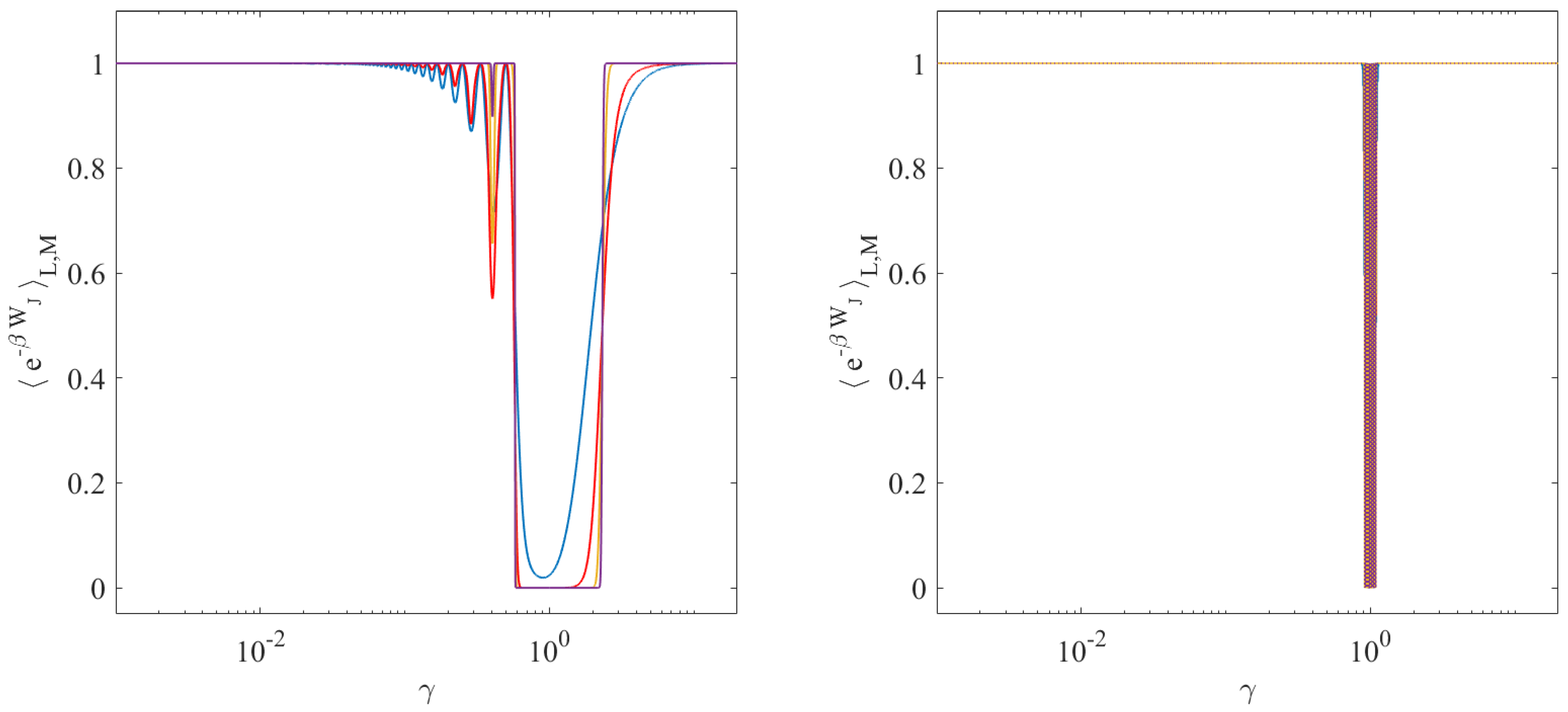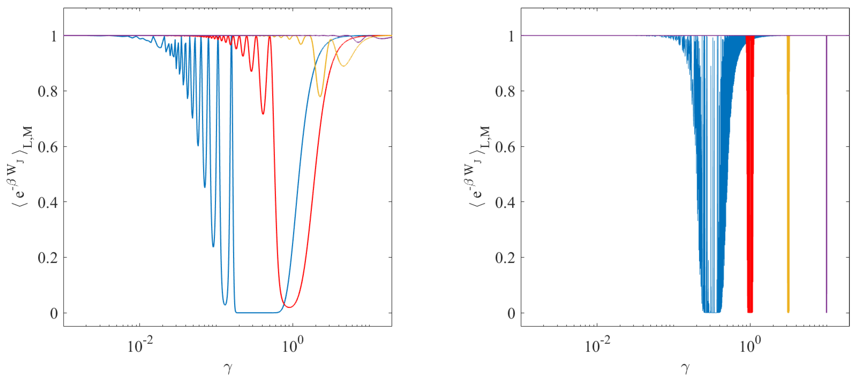Tuning the values of $\tau$, one observes quite a sensitive protocol dependence for the average (27). This is illustrated in Figure 1 and Figure 2. The cause of this behavior, in the presence of a resonance, is the fact that the amplitude of the oscillator position grows linearly in time, yielding the $\omega \tau$ term in the arguments of the error functions of $I_x^{\left(\mathrm{res}\right)}$.

3.3. Coupled Oscillators with Periodic Forcing

In this subsection, a single oscillator, S, is harmonically tied to the origin of the real line and is harmonically driven, as in Section 3.2. In addition, S is harmonically coupled to a second oscillator, E. We denote by $k_I$ the stiffness of the harmonic potential linking S and E, and we also assume that E is harmonically bound to the origin of the line, with elastic constant $k_E$. Let the oscillators masses be $m_E$ and $m_S$, and let the phase of S + E be denoted by $\mathrm{\Gamma }=\left(x_E,x_S,p_E,p_S\right)=\left(\mathbf{x},\mathbf{v}\right)$, where $p_E=m_E{v}_E$ and $p_S=m_S{v}_S$ are the momenta associated to each oscillator. Then, the Hamiltonian of the total system is given by:

$$\begin{array}{ccc}\hfill \mathcal{H}(\mathbf{x},\mathbf{v};\lambda )& =& \left[\frac{p_S^2}{2m_S}+\frac{k_S}{2}{x}_S^2+\frac{k_D}{2}{\left(\lambda -x_S\right)}^2\right]+\left[\frac{p_E^2}{2m_E}+\frac{k_E}{2}{x}_E^2\right]+\frac{k_I}{2}{(x_E-x_S)}^2\hfill \end{array}$$

(31)

$$\begin{array}{ccc}& =& H_S(x_S,p_S;\lambda )+H_E(x_E,p_E)+h_I\left(\mathbf{x}\right)\hfill \end{array}$$

(32)

where the square brackets delimit the different contributions to the full Hamiltonian, respectively, $H_S,H_E$, and $h_I$, as in Equation (1) for the JE theory. As the driving term, we take the periodic protocol used above: $sin\gamma t$, and we set again $k=k_S+k_D$. The equations of motion for this system are the following:

$$\begin{array}{c}\left\{\begin{array}{c}{m}_S{\ddot{x}}_S=-k{x}_S+k_{D}sin\gamma t-k_I\left(x_S-x_E\right),\\ m_E{\ddot{x}}_E=-k_E{x}_E-k_I\left(x_E-x_S\right),\end{array}\right.\hfill \end{array}$$

(33)

with initial conditions $\left(\mathbf{x}\left(0\right),\dot{\mathbf{x}}\left(0\right)\right)=\left({\mathbf{x}}_0,{\mathbf{v}}_0\right)={\mathrm{\Gamma }}_0$. Although analytical solutions for this set of equations are conceptually trivial, they are practically involved if $k_S\ne k_E$ and $m_S\ne m_E$, especially when integrated to compute the left-hand side of the JE. On the other hand, they can be quite simply handled in numerical calculations. We have thus numerically sampled the initial conditions ${\mathrm{\Gamma }}_0$ from the truncated canonical distribution, and for each of them, we have computed the initial energy $\mathcal{H}({\mathrm{\Gamma }}_0;\lambda \left(0\right))$. Then, we have numerically solved Equation (33) for that ${\mathrm{\Gamma }}_0$, obtaining the final condition ${\mathrm{\Gamma }}_{\tau }\left({\mathrm{\Gamma }}_0\right)$, that has been introduced in the final Hamiltonian $\mathcal{H}({\mathrm{\Gamma }}_{\tau }\left({\mathrm{\Gamma }}_0\right);\lambda \left(\tau \right))$, to obtain the work as:

$$W_J\left({\mathrm{\Gamma }}_0\right)=\mathcal{H}({\mathrm{\Gamma }}_{\tau }\left({\mathrm{\Gamma }}_0\right);\lambda \left(\tau \right))-\mathcal{H}({\mathrm{\Gamma }}_0;\lambda \left(0\right))$$

(34)

as in Equation (3), where $\lambda \left(0\right)=A=0$ and $\lambda \left(\tau \right)=sin\gamma \tau =B$. Collecting many works, with $\tau$ fixed, we have eventually estimated the quantity

$${〈e^{-\beta W_J}〉}_{0;L,M}$$

(35)

3.4. Results

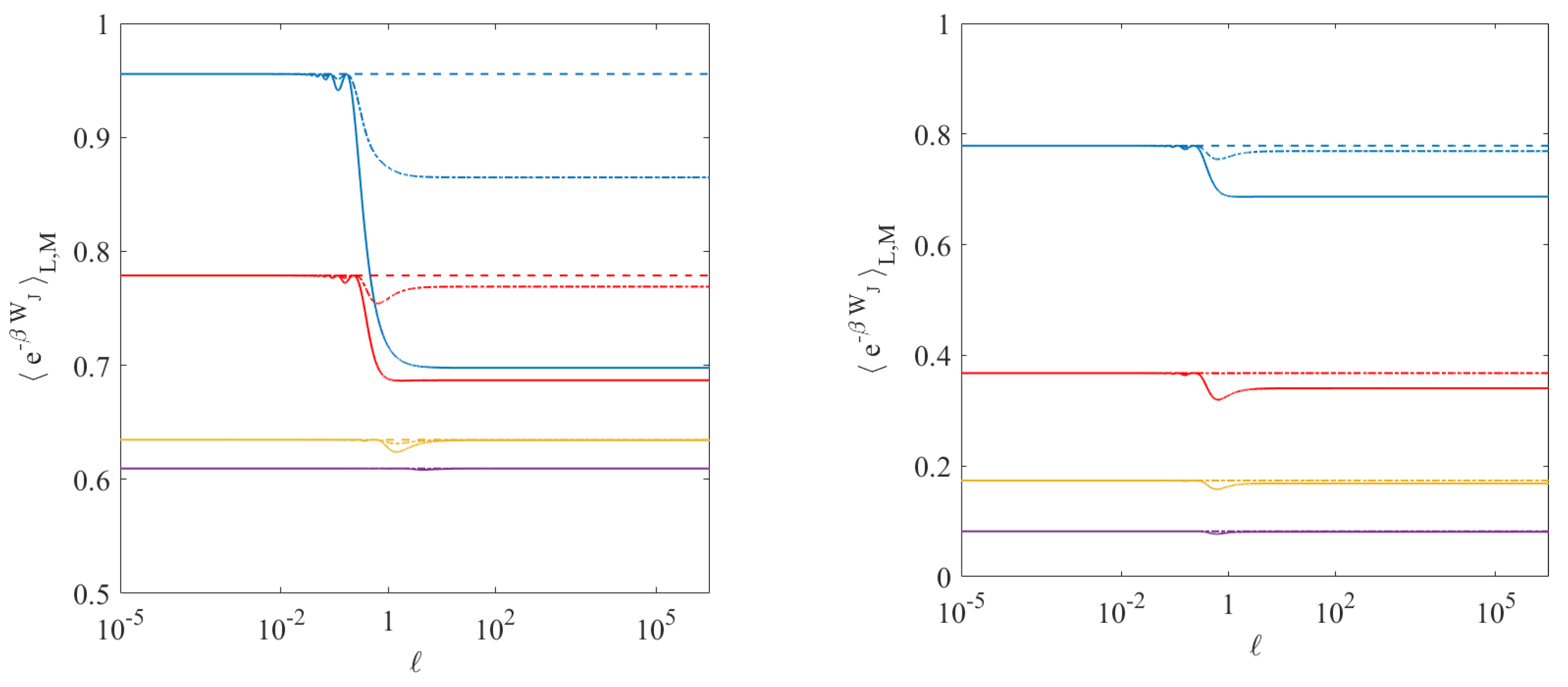
Our first observation is that finite size effects make the protocol on dependent the quantity (35), unlike the case of systems initially in contact with truly infinite reservoirs. Of course, no real reservoir is infinite, but considering it infinite introduces no errors when taking equilibrium averages of standard observables, such as power laws. The situation changes if the exponentials of standard observables are considered. For the single oscillator driven by a harmonic trap moving with constant velocity, Figure 3 shows the dependence of (35) on ℓ and on $\beta$, for different values of the harmonic potential stiffness $k_p$: fast and slow protocols yield different ensemble averages. The cases with $L=1$ and $M=1$, represented by solid lines, show an abrupt transition at about $\ell =1$, for small $k_p$. For large $k_p$, dominating the coupling with the driving agent, the result gradually turns independent of the speed of the process. Increasing the reservoir size to $L=5$ and $M=5$, the quantity (35) does not appear to depend anymore on the speed of the process $\lambda \left(t\right)$, cf. dashed lines in Figure 3. In reality, the dash-dotted lines for $L=M=2$ reveal that the process dependence merely shifts with L and M, becoming evident at larger ℓ. Therefore, process independence for (35) is only obtained when $L=\infty$ and $M=\infty$. Analogous behavior is observed as a function of the inverse temperature $\beta$, with more evident transitions at higher temperatures.

The second model analyzed above is even more intriguing, as resonances significantly affect the work done on the system by external perturbations when finite size effects play a role. Figure 1 and Figure 2 show that the extension of the phase space volume does not suffice to tame the resonances produced over sufficiently long times $\tau$. Unlike the case of infinitely large baths, which yield the same result for all $\tau$, here, a protocol dependence arises. The reason is that a harmonic oscillator subject to no friction and to periodic forces performs oscillations whose amplitude grows linearly in time if the forcing frequency equates to the natural frequency of the system. In our example, this happens for $\gamma =\omega$. Thus, the work done on the system grows together with the amplitude, pushing ${〈e^{-\beta W_J}〉}_{L,M}$ toward 0, at and near the resonance.

The inverse temperature $\beta$ and the global stiffness k of the potential also have noticeable effects on the behavior of (35). In particular, increasing $\beta$ (reducing the temperature) flattens the curve about the resonance, widening the interval of $\gamma$ values that make ${〈e^{-\beta W_J}〉}_{0;L,M}$ equal 0, rather than the infinite size theoretical value 1, cf. Figure 1. A larger value of k seems instead to stabilize ${〈e^{-\beta W_J}〉}_{0;L,M}$ and reduce its dependence on $\gamma$, as shown by Figure 2.

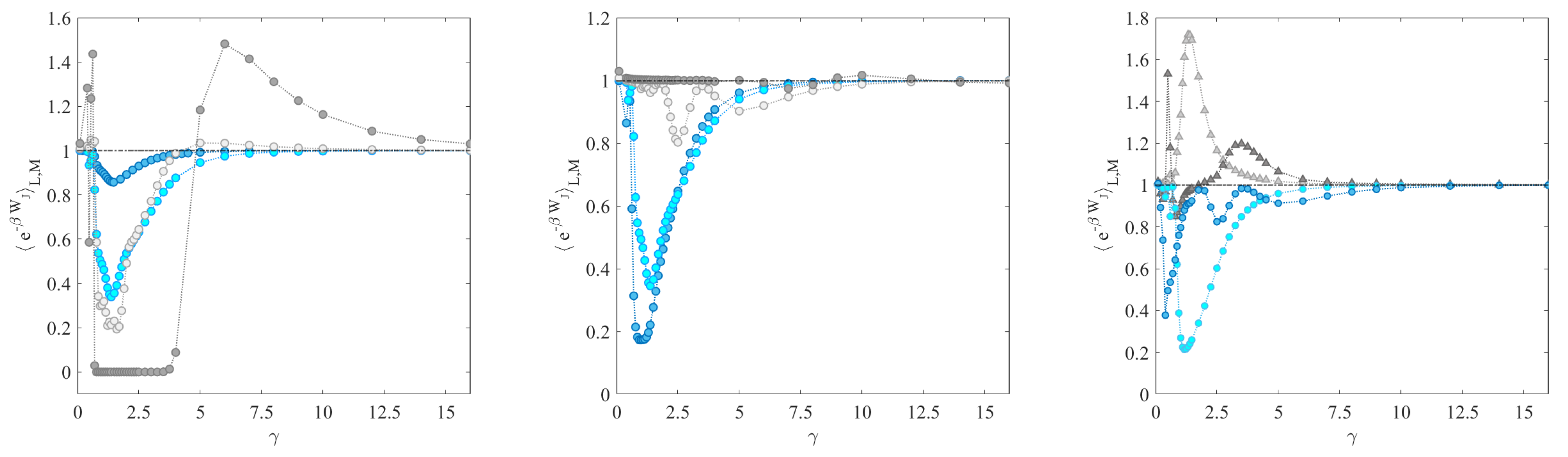
The pair of oscillators S and E from Section 3.3, with periodic forcing on S, shows a similar behavior, at least when the coupled particles have the same mass, $m_S=m_E=1$, and the interaction stiffness is sufficiently low (like $k_I=1$). This is illustrated by the first two panels of Figure 4, where the only parameters varied are $\beta$ and $k_S$. It is interesting to note how the temperature of the system needs to decrease (thus $\beta$ to increase) to make ${〈e^{-\beta W_J}〉}_{0;L,M}$ vanish. This is especially evident in the central panel of Figure 4 where none of the tested values of $k_S$ yields 0 for $\beta =1$. On the contrary, $\beta =100$ obtains ${〈e^{-\beta W_J}〉}_{L,M}=0$ for $k_S=1$ and different values of $\gamma$. The reason is that higher $\beta$ implies a narrower distribution, hence analogous to a case with smaller L and M.

Note that this is also relevant for infinite baths. A small temperature causes kinds of finite size effects due to the smallness of the distribution variance. That, assuming the infinite space can at least in principle be explored, may be eliminated only at the cost of collecting enormous statistics, which is often impossible. Therefore, the finite ensemble result remains only physically relevant.

The right panel of Figure 4 shows the quantity (35) computed on a variation of the coupled oscillators model, in which the “environment” mass $m_E$ is ten times bigger than the “system” mass $m_S$. To include possible effects due to the efficiency of the energy exchange between the system and environment, the stiffness of the interaction potential is varied: first, a value of $k_I=0.1$ is implemented, then $k_I=10$ is employed to account for a rapid exchange of energy between the parts, that result almost rigidly connected. The figures show that the two configurations generate similar results when the initial ensemble is restricted to $L=M=1$, while noticeably different behavior is observed for a larger system, where $L=M=5$. The rigidly coupled system produces oscillations of ${〈e^{-\beta W_J}〉}_{0;L,M}$ around the resonance frequency, with the loosely connected case exhibiting even more evident down-peaks in the values of ${〈e^{-\beta W_J}〉}_{L,M}$ about the resonance frequency, as in the case of the periodically forced single oscillator. Moreover, both $L=5=M$ lead to peaks that exceed 1. Both weakly and strongly coupled oscillators indicate that the presence of a massive environment drastically magnifies the finite size effects, noticeably deviating from the equality ${〈e^{-\beta W_J}〉}_{0;L,M}=1$.

4. Irreversible Expansion of an Ideal Gas

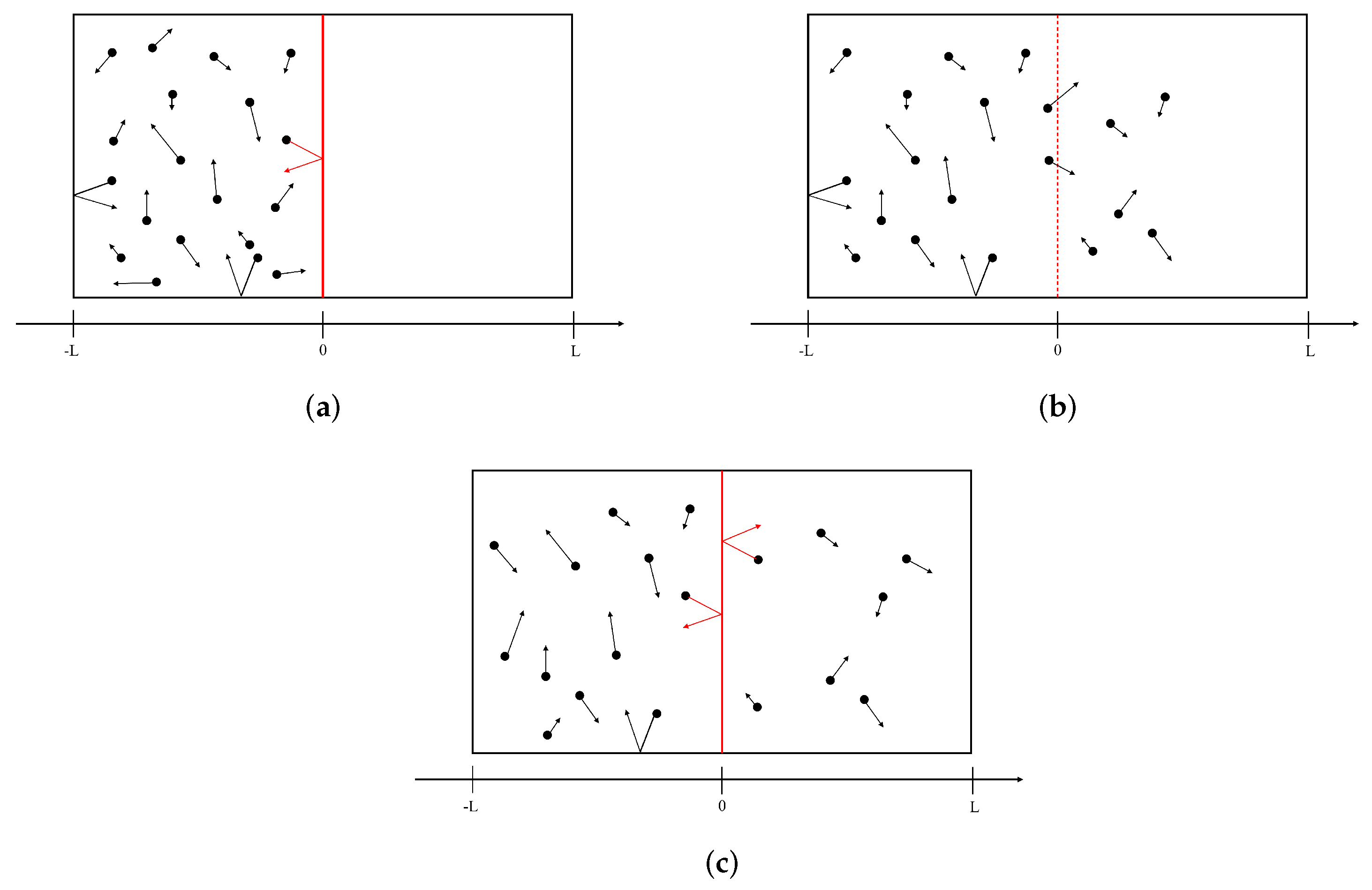
Consider a set of N identical point particles in a 2D rectangular box of length $2L$. The particles move in straight lines and collide elastically with the hard boundaries of the box. The box is subdivided into two equal parts by a wall perpendicular to two sides that can be removed and placed back according to prescribed protocols. We perform a cycle, starting from the gas confined by the wall in the left half of the box and in equilibrium at a given temperature T. At time $t=0$, the system is isolated from the bath, and the wall is removed for a certain amount of time $\tau$. Finally, the wall is placed back. A schematic representation of the system and its dynamics is given in Figure 5. The main observable here is the fraction of particles trapped in the right half of the box at the end of the cycle. Because this fraction depends on the details of the process through which the intermediate wall is removed and reinserted, the final equilibrium state may differ from the initial one and may depend on the protocol.

For the sake of simplicity and without any loss of significance, because the particles do not interact, we may replace the 2D container with a straight line segment of length $2L$. We also assume the particles to start with random initial positions, uniformly distributed in the interval $(-L,0)$, and with initial velocities normally distributed, with mean $\mu =0$ and standard deviation $\sigma =\sqrt{k_{B}T/m}$, where $k_B$ is the Boltzmann constant, T is the temperature of the bath and m is the mass of the particles. The fraction of particles escaping from the left half of the box to the right half, in the time interval $[0,\tau ]$, is obtained by integrating over all initial positions $x_0$ and initial velocities $v_0$ the probability for a particle to move from $(-L,0)$ to $(0,L)$. In the limit of many particles, the number of those leaving the left half and reaching the right half is this probability multiplied by their total number N. We denote by $N_L$ the number of particles in the left half of the box and by $N_R$ the number of those in the right half of the box so that $N=N_L+N_R$. Now, note that the initial velocities pointing rightward (i.e., $v_0>0$) that make a particle starting at $x_0\in (-L,0)$ end in $x_{\tau }\in (0,L)$ after a time $\tau$, fulfill the inequalities:

$$\frac{1}{\tau }(4nL-x_0)<v_0<\frac{1}{\tau }[(4n+2)L-x_0],n=0,1,2,\dots$$

(36)

because traveling a distance of $(4nL-x_0)$ brings the particle in the interval $(0,L)$, after a number n of bounces against the left wall of the container. Going beyond $[(4n+2)L-x_0]$ brings the same particle back to the left half of the box. The same reasoning, applied to particles initially pointing leftward (hence $v_0<0$), shows that a particle is found in the right half of the box at time $\tau$ if its velocity $v_0$ is such that:

$$-\frac{1}{\tau }[(4n+4)L+x_0]<v_0<-\frac{1}{\tau }[(4n+2)L+x_0),n=0,1,2,\dots$$

(37)

The number of particles residing in the right half of the box at time $\tau >0$, denoted as $N_R\left(\tau \right)$, is thus obtained by integrating over all initial positions $x_0$ in the interval $(-L,0)$ and overall initial velocities $v_0$ contained in the intervals given in (36) and (37). By doing this, one implicitly assumes the system is made of infinitely many particles; therefore, the result applies only for large N. For sufficiently large N, the following:

$$\frac{N_R\left(\tau \right)}{N}=\frac{1}{L\sigma \sqrt{2\pi }}{\int }_{-L}^0\mathrm{d}{x}_0\left\{\sum _{n=0}^{\infty }\left[{\int }_{\frac{1}{\tau }(4nL-x_0)}^{\frac{1}{\tau }[(4n+2)L-x_0]}{e}^{-v_0^2/2{\sigma }^2}\mathrm{d}{v}_0+{\int }_{\frac{1}{\tau }[(4n+2)L+x_0]}^{\frac{1}{\tau }[(4n+4)L+x_0]}{e}^{-v_0^2/2{\sigma }^2}\mathrm{d}{v}_0\right]\right\}$$

(38)

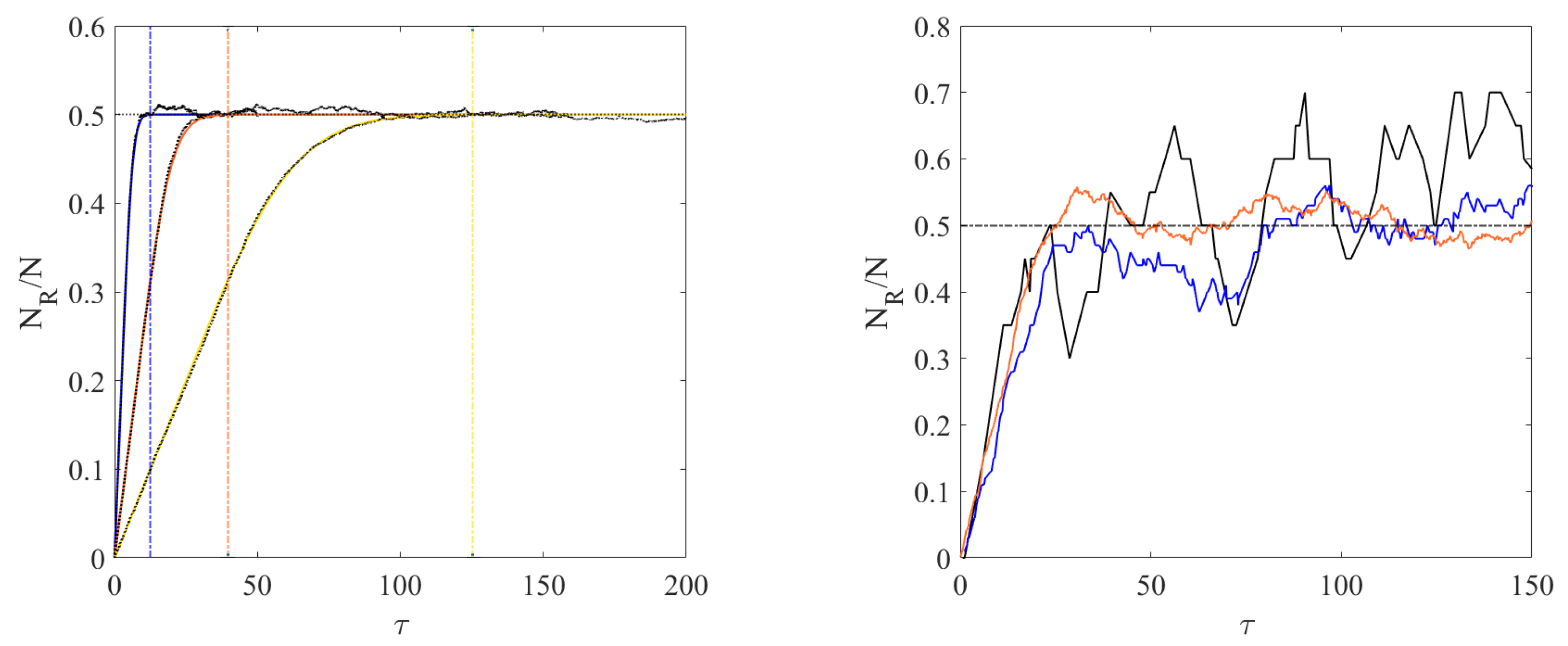
is thus an accurate prediction for observations. Then, integrating first over the velocity space, exchanging the integral over positions with the infinite sum (which is made possible since each term of the infinite sum is a continuous, bounded function), and finally integrating over initial positions, Equation (38) yields

$$\begin{array}{c}\hfill \begin{array}{ccc}\hfill \frac{N_R\left(\tau \right)}{N}& =\hfill & \frac{1}{2L}\sum _{n=0}^{\infty }\left\{\sqrt{\frac{2}{\pi }}\sigma \tau \left[exp\left(-\frac{16L^2{(n+1)}^2}{2{\sigma }^2{\tau }^2}\right)+exp\left(-\frac{16L^2{n}^2}{2{\sigma }^2{\tau }^2}\right)-2exp\left(-\frac{L^2{(4n+2)}^2}{2{\sigma }^2{\tau }^2}\right)\right]\right.\\ & & \left.-2(4n+2)Lerf\left[\frac{(4n+2)L}{\sqrt{2}\sigma \tau }\right]+4nLerf\left[\frac{4nL}{\sqrt{2}\sigma \tau }\right]+(4n+4)Lerf\left[\frac{(4n+4)L}{\sqrt{2}\sigma \tau }\right]\right\}\end{array}\end{array}$$

(39)

A comparison between this analytical result and numerical simulations of the system is shown in Figure 6. To estimate the relaxation times, in the absence of the intermediate wall, one cannot count on the mean time between two consecutive collisions with the boundaries of the box, given by $2L\langle 1/v\rangle$, because such a mean does not exist in a 1-dimensional space. However, one may take the distance $2L$ divided by the mean speed $\langle \left|v\right|\rangle$

$$\widehat{t}=\frac{2L}{\langle \left|v\right|\rangle }=\sqrt{2\pi }\frac{L}{\sigma }$$

(40)

as a characteristic time for the dynamics. This quantity estimates the time scale of the relaxation to a uniform distribution of particles when their number is sufficiently high that recurrence times can be considered infinite to all effects. As indicated by the vertical lines in the left panel of Figure 6, systems with larger $\beta$, i.e., smaller temperature, take longer to reach the uniform distribution of particles in the box, as expected.

The point here is that an irreversible process is generated by the motion of the moving wall, which returns to its initial position at the end of a cycle. The result is that variations of the processing time $\tau$ lead to different results for $N_R$, hence of the free energy of the final equilibrium states. For sufficiently large $\tau$, the process uniquely leads to $N_L=N_R$ (although fluctuations occur at any finite N, cf. the right panel of Figure 6), but that is different from the initial state $N_L=N$, $N_R=0$. Therefore, even accepting an ideal infinite thermostat, the variation of free energy between the initial and final state does not vanish and depends on the processing time $\tau$, at odds with the JE, i.e., with the canonical ensemble from which the JE is derived. In this case, the canonical distribution of momenta is given by a Gaussian. Were the range of momenta finite, further corrections to the canonical prediction would arise.

For the dynamics to be Hamiltonian, as the derivation of the JE requires, the wall could be modeled by a repulsive potential $\mathrm{\Phi }$, placed in the center of the box that diverges at time 0 and $\tau$, and that vanishes at time $\tau /2$. For instance, the following would do:

$$\mathsf{\Phi }(x;\lambda )=\left\{\begin{array}{cc}0\hfill & \hfill \mathrm{if}x\notin \left[1/2-ϵ,1/2+ϵ\right]\\ \frac{1}{\lambda }-\frac{4}{{\tau }^2}\hfill & \hfill \mathrm{if}x\in \left[1/2-ϵ,1/2+ϵ\right]\end{array}\right.\mathrm{with}\lambda \left(t\right)=t(\tau -t)$$

(41)

with $2ϵ>0$ representing the thickness of the wall. In this case, the infinitesimal contribution to $W_J$, given by the interaction of particle i in position $x_i$ with the wall, for a time $\mathrm{d}t$, is given by

$$\mathrm{d}{w}_i=\left\{\begin{array}{cc}0& \hfill \mathrm{if}{x}_i\notin \left[1/2-ϵ,1/2+ϵ\right]\\ \frac{2t-\tau }{t^2{(\tau -t)}^2}\mathrm{d}t& \hfill \mathrm{if}{x}_i\in \left[1/2-ϵ,1/2+ϵ\right]\end{array}\right.$$

(42)

which has to be integrated over the time intervals within $[0,\tau ]$ such that $x_i\in \left[1/2-ϵ,1/2+ϵ\right]$, and summed over all particles. Now, the standard canonical formalism is not applicable to this simple example because the phase space corresponding to the initial equilibrium state is altered when the wall potential is lowered to a finite height. It switches from representing an equilibrium state in half the volume of the box, to a different equilibrium state, that occupies the whole box. The instant in which the particles are allowed to move in the whole box but are still confined in its left half, the initial canonical distribution does not describe their state anymore and cannot be used to compute the free energy difference between the equilibrium states before and after the wall is removed. Nevertheless, this difficulty can be overcome, without affecting the result, considering, as generally and efficiently done (see e.g., Section 1.3 of Ref. [38]), that physically relevant space and time scales are finite, although they can be taken as large as one wants. Then, one realizes that a finite but high barrier confines a finite number of particles initially in the left half of the box, with only a negligible fraction $ϵ$ of them moving to the other half for a given time. A finite but higher barrier confines the particles with the same tolerance $ϵ$ for a larger time or for the same time and a smaller $ϵ$. Given the (arbitrarily large) time and the (arbitrarily small) tolerance considered physically satisfactory, there is a barrier height that produces better confinement, allowing the initial state to be considered an equilibrium state. Then, the protocol dependence of the free energy difference described above remains.

5. Concluding Remarks

In this work, we have discussed simple examples concerning finite size effects and a broken time-reversal symmetry on the calculations of values of observables within the statistical mechanics formalism. It is indeed ever more important to properly describe systems that do not lie within the traditional bounds of statistical mechanics, developed for macroscopic systems at equilibrium or slowly evolving near equilibrium states. Indeed, contemporary research widely focuses on small and far-from-equilibrium systems. In the case of equilibrium macroscopic systems, the use of the standard ensembles is fully justified because the observables of interest are determined by the bulk, not the tails of the probability distributions. This approach is validated both by theory and experiments. On the contrary, fluctuations of properties of interest in the case of small or strongly nonequilibrium systems can compare to average signals and require a proper characterization of the tails of the distributions, which may also be affected by a spontaneous time-reversal symmetry breaking, not evident in the equations of motion. Indeed, the interaction with heat reservoirs is often limited to processes that last very short times, making effective only small parts of such environments. To illustrate these points, we have investigated simple driven harmonic oscillator systems, averaging the popular quantity $exp(-\beta W_J)$ with canonical and truncated canonical averages. We have shown that:

• A single oscillator pulled by a constant speed harmonic trap yields the infinite bath result if the process is not too fast. It sensibly and rapidly departs from that when the speed of the driving agent grows. The effect is more evident (as expected) for small than for large integration bounds, L and M, for smaller harmonic constants, and for smaller bath temperatures. In the infinite $L,M$ limits, the standard canonical result is recovered, but larger and larger L and M are required; the smaller are $k_p$ or $\beta$.
• For a single periodically driven oscillator, the infinite bath result over a multiple of the driving period equals 1. Strong deviations from this value, even those that reach 0, are found for a finite bath in finite intervals about the resonance frequency. Although the theoretical result is again obtained in the infinite $L,M$ limit, this is harder if the driving acts for longer times (i.e., for a larger number of periods).
• In the case in which the oscillator S is coupled to an oscillator E, the infinite bath value 1 is obtained, apart from oscillations, for a sufficiently large driving frequency. Noticeable deviations from that results are still present about specific values of the forcing frequency. In this case, we have no analytical expression for the finite bath result. Therefore this conclusion is based on numerical data for a finite ensemble of initial conditions, proven robust against variations of ensemble size.

The last example we have considered implies the breaking of the classical time-reversal symmetry and consists of an ideal gas initially in equilibrium with an infinite thermal bath at temperature T, which is confined in the left half of its container by a moving barrier. Initially, the barrier confines all particles to the left half of the container, and that allows an equilibrium state, represented by a uniform distribution for the positions of particles in $[-L,0]$ and a Gaussian distribution for their velocities. As soon as the barrier allows particles to reach the right half of the container, the phase space changes to one in which positions cover the $[-L,L]$ interval, and the initial ensemble immediately fails to represent an equilibrium state. The observables take instead some time to change. This prevents the application of the standard statistical mechanical formalism because the phase space of the equilibrium initial state is not the one of the nonequilibrium evolution, and, for instance, the Liouville equation fails. A modification in time of the volume of a given system to the very least requires a suitable time-dependent scaling of the phase space coordinates [39] for the formalism to apply but that is not possible in our case, because the volume changes instantaneously. Nevertheless, the experiment can be performed, and a proper formalism for it has been identified in terms of finite potential barriers and time scales.

Discrepancies between canonical formalism and experimental situations are known to arise when irreversibility emerges: they are intrinsic and not merely due to insufficient statistics. All boils down to the conclusion that finite size and irreversibility effects similarly lead to protocol-dependent averages of exponential quantities such as $exp(-\beta W_J)$. The standard statistical mechanics’ formalism should be adapted to treat these cases. This fits nicely with the standard statistical mechanical justification of ensembles. For instance, in Ref. [35], Fermi states:

Studying the thermodynamical state of a homogeneous fluid of a given volume at a given temperature […], we observe that there is an infinite number of states of molecular motion that correspond to it. With increasing time, the system exists successively in all the dynamical states that correspond to the given thermodynamical state. From this point of view, we may say that a thermodynamical state is the ensemble of all the dynamical states through which, as a result of the molecular motion, the system is rapidly passing.

and Callen adds

If the transition mechanism among the atomic states is sufficiently effective, the system passes rapidly through all representative atomic states in the course of a macroscopic observation […]. However, under certain unique conditions, the mechanism of atomic transition may be ineffective, and the system may be trapped in a small subset of atypical atomic states. Or, even if the system is not completely trapped, the rate of transition may be so slow that a macroscopic measurement does not yield a proper average over all possible atomic states.

In reality, less than what is required by Fermi and Callen is needed for ensembles to work because observables of interest are generally a few and well-behaved [37,40,41]. However, when the standard conditions are severely violated, and the observables call for an accurate representation of large fluctuations, canonical results must be taken with a grain of salt.