Bipolar b-Metric Spaces in Graph Setting and Related Fixed Points

Abstract

In this article, we develop a new notion that combines fixed-point theory and graph theory: graphical bipolar b-metric spaces. We demonstrate fixed-point solutions in the framework of graphical bipolar b-metric spaces, employing covariant and contravariant mapping contractions, which is a new addition to this end. This article also features illustrative examples drawn from various contexts to further demonstrate our findings. This is a significant study since it melds ideas from graph theory with those from generalized bipolar metric spaces, and considers that the symmetry of the edges of the underlying graphs connected with the enunciated metric spaces is essential in the graphical metric spaces.

1. Introduction

Fixed-point theory ($\mathtt{FPT}$), which serves as a bridge between topology and analysis, is a fundamental and commonly used tool in modern mathematics. It investigates the circumstances in which a self-map on a non-empty set admits one or more fixed points. $\mathtt{FPT}$ is divided into three categories: metric $\mathtt{FPT}$, topological $\mathtt{FPT}$, and discrete $\mathtt{FPT}$. This field’s researchers operate in a variety of directions and generalize their findings. Poincare and Brouwer made substantial contributions to this field, particularly Brouwer’s (topological) fixed-point theorem. The metric fixed-point theorem rose to popularity due to its applications in both pure and applied mathematics, particularly in determining the presence of solutions to nonlinear systems. Banach’s contraction principle, established in 1922, is a noteworthy achievement in $\mathtt{FPT}$ and approximation theory, and it is well respected for its adaptability.

In $\mathtt{FPT}$, the concept of metric space ($\mathtt{MS}$) and the Banach contraction principle ($\mathtt{BCP}$) are fundamental. Many scholars have been drawn to metric spaces ($\mathtt{MSs}$) because of their axiomatic clarity. Several writers have generalized the $\mathtt{BCP}$ by using various forms of contraction mappings in different $\mathtt{MSs}$ (for example, [1,2]). Mutlu and Gürdal [3] introduced the concept of bipolar $\mathtt{MS}$ in 2016, which is a type of partial distance that connects $\mathtt{MSs}$ and bipolar $\mathtt{MSs}$. After that, Mutlu and Ozkan generalized coupled fixed-point theorems in bipolar $\mathtt{MSs}$ in 2017 [4]. Furthermore, Gürdal et al. extended fixed-point results to multivalued mappings in these spaces in 2020 [5]. Researchers interested in an in-depth analysis may refer to [6,7].

Many researchers are concentrating on the field of graphical $\mathtt{FPT}$, as evidenced by pioneering articles such as [8,9,10,11]. Graph theory has become increasingly significant in the study of $\mathtt{FPT}$. For solving DEs with infinite delay, Hammad and Zayed [12] used fixed-point analysis on b-$\mathtt{MS}$ in conjunction with graph symmetry, while Shukla et al. defined graphical $\mathtt{MSs}$ [13], and Chuensupantharat et al. [8] defined graphical b-$\mathtt{MSs}$ with accompanying graphs. In 2019, Younis et al. expanded on previous work by extending these notions to graphical rectangular b-$\mathtt{MSs}$ and controlled-graphical $\mathtt{MSs}$ [11,14]. Hooda et al. [15] provided a good summary of the literature on b-$\mathtt{MSs}$ and their generalized forms. The authors emphasized specific ordered vector spaces derived from the b-$\mathtt{MSs}$ and discussed their relevance in economic research. Then, using a graph endowed with edge symmetry, they built shared fixed-point outcomes on the vector b-$\mathtt{MSs}$. Popescu [16], on the other hand, used the graphic contraction principle to deal with a new type of operator and produced fixed-point theorems that complement prior discoveries in nonlinear operator theory. A connection is shown between iterative techniques and Ulam–Hyers stability issues in particular. The illuminating article given in [17] provides a comprehensive explanation of graphical structures.

Considering the aforementioned discussion, in this article, we establish the notion of graphical structure in bipolar b-$\mathtt{MSs}$, which is a generalization of bipolar $\mathtt{MSs}$, prompted by the existing literature and following the work of Younis et al. and Mutlu and Gürdal [3,11]. We demonstrate the correctness of fixed-point theorems by using covariant and contravariant mapping contractions, respectively, and give examples with different cases.

2. Preliminaries

In this part of the article, we will discuss some primary definitions and certain primary facts necessary for the continued examination of the subject.

Consider $\mathsf{\Theta }=\left(V\right(\mathsf{\Theta }),E(\mathsf{\Theta }\left)\right)$, a digraph having no parallel edges carrying $\Delta$ as a diagonal of $Ł\times Ł$, $\varphi \ne Ł.$ It is assumed that the vertex set (node-set) $V\left(\mathsf{\Theta }\right)$ coincides with the set Ł, whereas $E\left(\mathsf{\Theta }\right)$ is equipped with all the loops of the graph.

We refer to the graph with symmetric edges as $\breve{\mathsf{\Theta }}$ (graph symmetry). With this concept, we have

$$E({\mathsf{\Theta }}^{-1})\cup E(\mathsf{\Theta })=E(\breve{\mathsf{\Theta }}),$$

where ${\mathsf{\Theta }}^{-1}$ is a symmetric graph obtained by inverting the edges of $\theta .$

Let us say that the nodes of the digraph $\mathsf{\Theta }$ are $\kappa$ and w. A sequence ${\left\{{\kappa }_j\right\}}_{j=0}^m$ with $(1+m)$ nodes is a path in $\mathsf{\Theta }$ if the following contends:

$${\kappa }_0=\kappa ,{\kappa }_m=w\mathrm{such}\mathrm{that}({\kappa }_{j-1},{\kappa }_j)\in E\left(\mathsf{\Theta }\right);j=1,2,\dots ,m.$$

If a path connects a node of $\mathsf{\Theta }$ to every other node, we say $\mathsf{\Theta }$ is connected. In the case of a graph, $\mathsf{\Theta }$ is undirected and possesses a path between its very pair of nodes; we call $\mathsf{\Theta }$ to be a weakly connected graph. A graph $H=\left(V\left(H\right),E\left(H\right)\right)$ is considered to be a sub-graph of $\mathsf{\Theta }$ if $V\left(H\right)\subseteq V\left(\mathsf{\Theta }\right)$ and $E\left(H\right)\subseteq E\left(\mathsf{\Theta }\right)$.

On the other side, a novel development in graph-metric theory was introduced by Shukla [13], where the authors used the following notions:

• ${\left[\kappa \right]}_{\mathsf{\Theta }}^l$ consists of the set of all nodes $w\in$ Ł making a directed path from $\kappa$ in $\mathsf{\Theta }$ with length l.
• The symbol P represents a relation on Ł with ${\left(\kappa Pw\right)}_{\mathsf{\Theta }}$ representing that there is a path from $\kappa$ to w in the graph $\mathsf{\Theta }$.
• If $w\in {\left(\kappa Pw\right)}_{\mathsf{\Theta }}$, then w is somewhere on the path ${\left(\kappa Pw\right)}_{\mathsf{\Theta }}$.

Additionally, we say a sequence $\left\{{\kappa }_m\right\}\subset Ł$ is $\mathsf{\Theta }-$term-wise-connected ($\mathsf{\Theta }-TWC$) if ${\left({\kappa }_{m}P{\kappa }_{m+1}\right)}_{\mathsf{\Theta }}$ for all $m\in \mathbb{N}$. Unless otherwise specified, all graphs will thereafter be interpreted as being directed.

Bipolar $\mathtt{MSs}$ are a new kind of partial distance introduced by Mutlu and Gürdal [3]. In particular, they focus on the completeness of $\mathtt{MSs}$ and their connection to bipolar $\mathtt{MSs}$. The following is the formal definition.

Definition 1

([3]). A bipolar $\mathtt{MS}$ is triple $(Ł, {Ł}^{*}, d)$ such that $Ł,{Ł}^{*}\ne \varphi$ and $d:Ł\times {Ł}^{*}\to {\mathbb{R}}^{+}$ is a function satisfying the underlying properties:

1. 

If $d(\partial ,ð)=0,$ then $\partial =ð,$ $(\partial ,ð)\in Ł\times {Ł}^{*}.$

2. 

If $\partial =ð,$ then $d(\partial ,ð)=0,$ $(\partial ,ð)\in Ł\times {Ł}^{*}.$

3. 

$d(\partial ,ð)=d(ð,\partial ),$ for all $\partial ,ð\in Ł\cap {Ł}^{*}.$

4. 

$d({\partial }_1,{ð}_2)\le d({\partial }_1,{ð}_1)+d({\partial }_2,{ð}_1)+d({\partial }_2,{ð}_2),$

for all ${\partial }_1,{\partial }_2\in Ł$,${ð}_1,{ð}_2\in {Ł}^{*}$ and ${\mathbb{R}}^{+}$ is set of all non-negative real numbers. Then, d is called a bipolar $\mathtt{MS}$ on the pair $(Ł,{Ł}^{*}).$

The following characteristics are listed following the aforementioned definition:

(i)

If conditions (2) and (3) are satisfied, d is referred to as a bipolar pseudo-semi metric on the pair $(Ł,{Ł}^{*})$.

(ii)

A bipolar pseudo-metric ($\mathtt{BPSM}$) is one where d is a bipolar pseudo-semi metric meeting (4).

(iii)

A bipolar metric is a $\mathtt{BPSM}$ d satisfying (2).

A triple $(Ł,{Ł}^{*},d)$, where d is a bipolar (pseudo-(semi)) metric on $(Ł,{Ł}^{*})$, is referred to as a bipolar (pseudo-(semi)) $\mathtt{MS}$. Specifically, the space is referred to as a disjoint if $Ł\cap {Ł}^{*}=\varphi$; otherwise, it is referred to as a joint. The left and right poles of $(Ł,{Ł}^{*},d)$ are the sets L and $L\ast$, respectively.

A $\mathtt{BPSM}$ typically only considers the distance between points that are in different poles of space. It also reveals some details about these poles’ internal structure.

Example 1

([3]). The following are some examples related to the defined terms:

(i) 

If $(Ł,{Ł}^{*})$ is a (pseudo-(semi)) $\mathtt{MS}$ with distance function d, then $(Ł,{Ł}^{*},d)$ is a bipolar (pseudo-(semi)) $\mathtt{MS}$. Conversely, if $(Ł,{Ł}^{*},d)$ is a bipolar (pseudo-(semi)) $\mathtt{MS}$ with $Ł={Ł}^{*}$, then $(Ł,{Ł}^{*})$ is also a (pseudo-(semi)) $\mathtt{MS}$.

(ii) 

In a quasi-$\mathtt{MS}$ $(Ł,{Ł}^{*})$, if we define the set ${Ł}^{*}=Ł\times Ł$, then $(Ł,{Ł}^{*},d^{\prime })$ is a disjoint bipolar $\mathtt{MS}$, where $d^{\prime }({\partial }_1,({\partial }_2,Ł))=d({\partial }_1,{\partial }_2)$ for every ${\partial }_1,{\partial }_2\in Ł$. The axiom of regularity requires that the sets Ł and ${Ł}^{*}$ be disjoint.

(iii) 

Let Ł be a set, and d be a pseudo-semimetric on Ł with the property that $Ł\cap P\left(Ł\right)=\varnothing$. The point-to-set distance function $d^{\prime }:Ł\times P\left(Ł\right)\to {\mathbb{R}}^{+}$ is a bipolar pseudo-semimetric on the pair $(Ł,P(Ł\left)\right)$.

(iv) 

Consider the nonempty sets Ł and ${Ł}^{*}$, a pseudo-$\mathtt{MS}$ $(Z,\rho )$, and a function $f:Ł\cup {Ł}^{*}\to Z$. The function $d:Ł\times {Ł}^{*}\to {\mathbb{R}}^{+}$ defined as $d(\partial ,ð)=\rho \left(f\right(\partial ),f(ð\left)\right)$ represents a $\mathtt{BPSM}$ on $(Ł,{Ł}^{*})$. If Ł and ${Ł}^{*}$ are normed spaces, then $d(\partial ,ð)=\left|\left|\right|\partial \left|\right|-\left|\right|ð\left|\right|\right|$ denotes a $\mathtt{BPSM}$ on $(Ł,{Ł}^{*})$.

(v) 

Let C represent the set of all functions, $f:\mathbb{R}\to [1,3]$, and $d:C\times \mathbb{R}\to {\mathbb{R}}^{+}$ can be defined as $d(f,\partial )=f(\partial )$. The space $(C,\mathbb{R},d)$ is a disjoint bipolar $\mathtt{MS}$.

Definition 2

([4]). Let $({Ł}_1,{Ł}_1^{*})$ and $({Ł}_2,{Ł}_2^{*})$ be two sets and consider a mapping $T:{Ł}_1\cup {Ł}_1^{*}\rightrightarrows {Ł}_2\cup {Ł}_2^{*}$; then, T is called a covariant ($\mathtt{CoVM}$) if T fulfills the underlying property:

$$T\left({Ł}_1\right)\subseteq {Ł}_2\mathrm{and}T\left({Ł}_1^{*}\right)\subseteq {Ł}_2^{*}.$$

On the other hand, T is called a contravariant mapping ($\mathtt{CnVM}$) if the following condition is met:

$$T\left({Ł}_1\right)\subseteq {Ł}_2^{*}\mathrm{and}T\left({Ł}_1^{*}\right)\subseteq {Ł}_2.$$

Such types of mappings are denoted by $T:({Ł}_1,{Ł}_1^{*})\rightleftarrows ({Ł}_2,{Ł}_2^{*})$. One should take care that $d_1$ and $d_2$ are bipolar $\mathtt{MSs}$ on $({Ł}_1,{Ł}_1^{*})$ and $({Ł}_2,{Ł}_2^{*})$, respectively.

Definition 3

([5]). Suppose $(Ł,{Ł}^{*},d)$ is a bipolar $\mathtt{MS}$. A point $\kappa \in Ł\cup {Ł}^{*}$ is the left point if $\kappa \in Ł,$ the right point if $\kappa \in {Ł}^{*}$ and a central point if $\kappa \in Ł\cap {Ł}^{*}.$ A sequence $\left({\partial }_n\right)$ on Ł is the left sequence and $\left({ð}_n\right)$ on ${Ł}^{*}$ is the right sequence. A left or right sequence is simply a sequence in $(Ł,{Ł}^{*},d).$ A sequence $\left({\kappa }_n\right)$ is said to be convergent to a point κ; if $\left({\kappa }_n\right)$ is the left sequence and κ is the right point, then $\underset{n\to \infty }{lim}d({\kappa }_n,\kappa )=0.$ Similarly, if $\left({\kappa }_n\right)$ is the right sequence and κ is the left point, then $\underset{n\to \infty }{lim}d(\kappa ,{\kappa }_n)=0.$ A sequence $({\partial }_n,{ð}_n)\in Ł\times {Ł}^{*},$ is said to be a bi-sequence $\left(BC\right)$ on $(Ł,{Ł}^{*},d).$ If both sequences $\left({\partial }_n\right)$ and $\left({ð}_n\right)$ converge, then the $BC$ is said to be bi-convergent, and if both sequences converge to the same point $\kappa \in Ł\cap {Ł}^{*},$ then $BC$ is said to be bi-convergent. Every bi-convergent $BC$ in $(Ł,{Ł}^{*},d)$ is a Cauchy $BC$, and every convergent $BC$ is bi-convergent.

Definition 4

([3]). Let $({Ł}_1,{Ł}_1^{*},d_1)$ and $({Ł}_2,{Ł}_2^{*},d_2)$ be a bipolar $\mathtt{MS}$. A mapping T is continuous if it is left continuous at each point $\partial \in {Ł}_1$ and right continuous at each point $ð\in {Ł}_1^{*}$. A $\mathtt{CnVM}$ $T:({Ł}_1,{Ł}_1^{*})\rightleftarrows ({Ł}_2,{Ł}_2^{*})$ is continuous if and only if it is continuous as a $\mathtt{CoVM}$ $T:({Ł}_1,{Ł}_1^{*})\rightrightarrows ({Ł}_2,{Ł}_2^{*})$.

It can be seen from Definition 3 that a covariant or a $\mathtt{CnVM}$ is continuous if and only if $\left({\partial }_n\right)\to ð$ on $({Ł}_1,{Ł}_1^{*},d_1)$, implying that $T\left({\partial }_n\right)\to T\left(ð\right)$ on $({Ł}_2,{Ł}_2^{*},d_2)$.

3. Graphical Bipolar b-$\mathtt{MSs}$

In this section, we introduce the notion of graphical bipolar b-$\mathtt{MS}$ $(Ł,{Ł}^{*},d_{\mathsf{\Theta }})$ as follows:

Definition 5.

Consider a metric $d_{\mathsf{\Theta }}:Ł\times {Ł}^{*}\to {\mathbb{R}}^{+},$ endowed with the graph Θ with Ł$,{Ł}^{*}\ne \varphi$ and $b\ge 1$, contending the following axioms:

1. 

If $d_{\mathsf{\Theta }}(\partial ,ð)=0,$ then $\partial =ð.$

2. 

If $\partial =ð,$ then $d_{\mathsf{\Theta }}(\partial ,ð)=0.$

3. 

$d_{\mathsf{\Theta }}(\partial ,ð)=d_{\mathsf{\Theta }}(ð,\partial ),$ for all $\partial ,ð\in Ł\cap {Ł}^{*}.$

4. 

${\left({\partial }_{1}P{ð}_2\right)}_{\mathsf{\Theta }},$${\partial }_2,{ð}_1\in {\left({\partial }_{1}P{ð}_2\right)}_{\mathsf{\Theta }}$$\Rightarrow d_{\mathsf{\Theta }}({\partial }_1,{ð}_2)\le b[d_{\mathsf{\Theta }}({\partial }_1,{ð}_1)+d_{\mathsf{\Theta }}({\partial }_2,{ð}_1)+d_{\mathsf{\Theta }}({\partial }_2,{ð}_2)]$,

for all ${\partial }_1,{\partial }_2\in Ł$ and ${ð}_1,{ð}_2\in {Ł}^{*}$, where $(\partial ,ð)\in Ł\times {Ł}^{*}.$

A triplet $(Ł,{Ł}^{*},d_{\mathsf{\Theta }})$ is called a graphical bipolar b-$\mathtt{MS}$ if $d_{\mathsf{\Theta }}$ satisfies the postulates (1–4).

Remark 1.

It is noteworthy that graphical bipolar b-$\mathtt{MS}$ $(Ł,{Ł}^{*},d_{\mathsf{\Theta }})$ is the generalization of bipolar $\mathtt{MS}$ $(Ł,{Ł}^{*},d)$ if we take $b=1$.

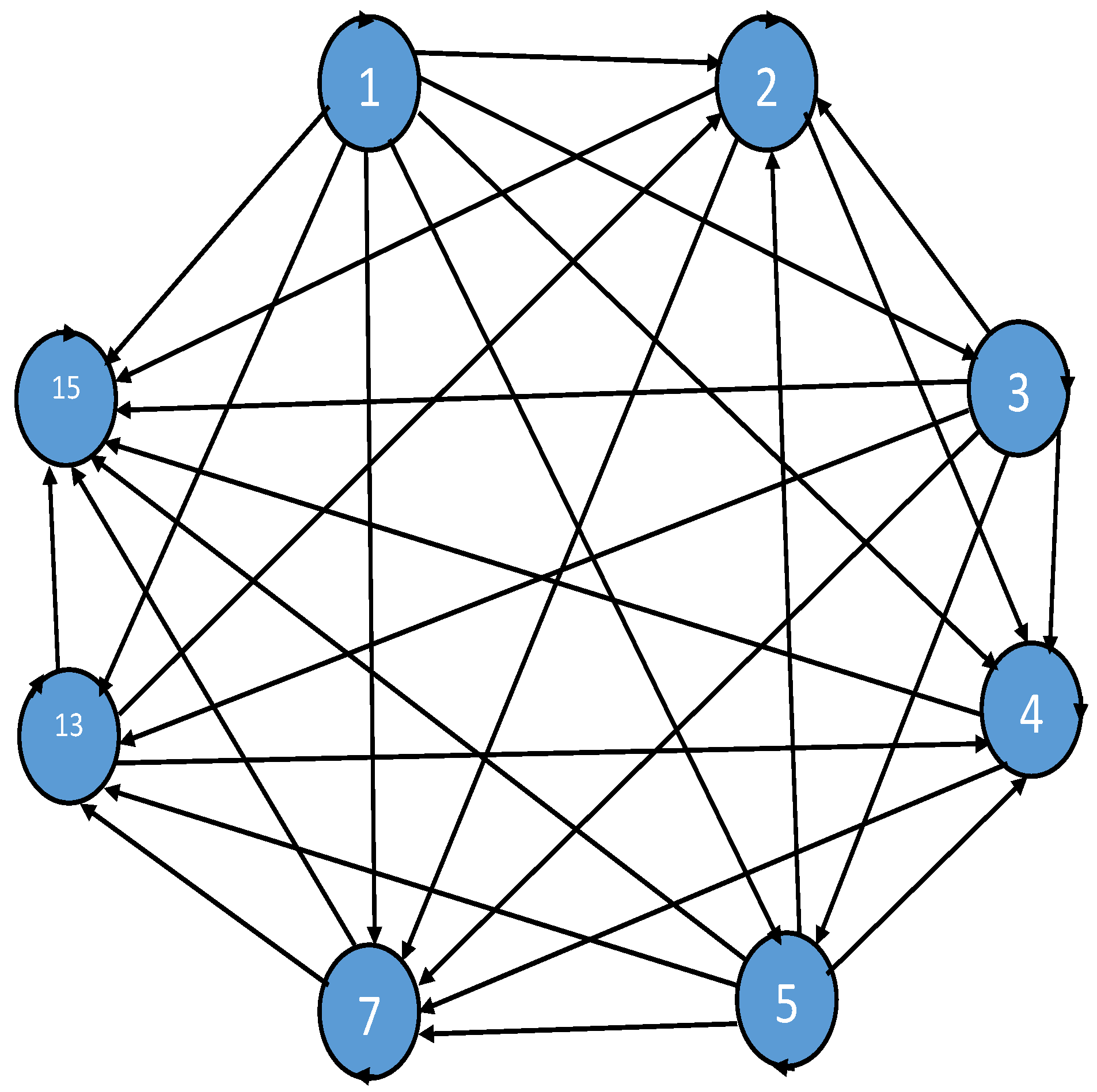
Example 2.

Let $Ł=\{1,3,5,7,13\}$, ${Ł}^{*}=\{2,4,5,7,15\}$, and the function $d_{\mathsf{\Theta }}:Ł\times {Ł}^{*}\to {\mathbb{R}}^{+}$ is defined as

$$d_{\mathsf{\Theta }}(\partial ,ð)=\left\{\begin{array}{c}0,if\partial =ð\\ min\{\partial ,ð\},otherwise,\end{array}\right.$$

where $b=\frac{13}{4}$ for all $\partial \in Ł$, $ð\in {Ł}^{*}$ and equipped with graph $\mathsf{\Theta }.$ The graph $\mathsf{\Theta }=\left(V\right(\mathsf{\Theta }),E(\mathsf{\Theta }\left)\right)$, having the set of vertices

$$V\left(\mathsf{\Theta }\right)=Ł\cup {Ł}^{*}=\{1,2,3,4,5,7,13,15\},$$

and the set of edges given by the following:

$$E\left(\mathsf{\Theta }\right)=▵\cup \left\{\begin{array}{c}(1,2),(1,3),(1,4),(1,5),(1,7),(1,13),\\ (1,15),(3,2),(2,4),(5,2),(2,7),(13,2),\\ (2,15),(3,4),(3,5),(3,7),(3,13),(3,15),\\ (5,4),(4,7),(13,4),(4,15),(5,7),(5,13),\\ (5,15),(7,13),(7,15),(13,15).\end{array}\right\}$$

The corresponding edges of the graph Θ are propounded in Figure 1.

In order to verify that $(Ł,{Ł}^{*},d_{\mathsf{\Theta }})$ is graphical bipolar b-$\mathtt{MS}$, we discuss some cases for validating the underlying inequality of Definition 5.

$$d_{\mathsf{\Theta }}({\partial }_1,{ð}_2)\le b[d_{\mathsf{\Theta }}({\partial }_1,{ð}_1)+d_{\mathsf{\Theta }}({\partial }_2,{ð}_1)+d_{\mathsf{\Theta }}({\partial }_2,{ð}_2)].$$

(1)

Case (i): If we take ${\partial }_1=13,$ ${\partial }_2=1,$ ${ð}_1=2,$ and ${ð}_2=15$, we have

$$\begin{array}{ccc}\hfill d_{\mathsf{\Theta }}(13,15)& \le & b[d_{\mathsf{\Theta }}(13,2)+d_{\mathsf{\Theta }}(1,2)+d_{\mathsf{\Theta }}(1,15)]\hfill \\ \hfill 13& \le & b\left(4\right).\hfill \end{array}$$

Consequently, for $b=\frac{13}{4}$, (1) holds.

Case (ii): If ${\partial }_1=1,$ ${\partial }_2=13,$ ${ð}_1=4,$ and ${ð}_2=2,$ then

$$\begin{array}{ccc}\hfill d_{\mathsf{\Theta }}(1,2)& \le & b[(1,4)+d_{\mathsf{\Theta }}(13,4)+d_{\mathsf{\Theta }}(13,2)]\hfill \\ \hfill 7& \le & b\left(7\right).\hfill \end{array}$$

This amounts to saying that (1) holds for $b=\frac{13}{4}$.

Case (iii): When ${\partial }_1=3,$ ${\partial }_2=5,$ ${ð}_1=2,$ and ${ð}_2=4,$ we find

$$\begin{array}{ccc}\hfill d_{\mathsf{\Theta }}(3,4)& \le & b[d_{\mathsf{\Theta }}(3,2)+d_{\mathsf{\Theta }}(5,2)+d_{\mathsf{\Theta }}(5,4)]\hfill \\ \hfill 3& \le & b\left(6\right).\hfill \end{array}$$

Evidently, (1) is valid for $b=\frac{13}{4}$.

For different cases, we adopt the same analysis to infer that $(Ł,{Ł}^{*},d_{\mathsf{\Theta }})$ is a graphical bipolar b-$\mathtt{MS}$ with $b=\frac{13}{4}$.

Figure 1. Underlying graph.

Figure 1. Underlying graph.

Definition 6.

Let $f:{Ł}_1\cup {Ł}_1^{*}\to {Ł}_2\cup {Ł}_2^{*}$ be a function on pairs of sets $({Ł}_1,{Ł}_1^{*})$ and $({Ł}_2,{Ł}_2^{*})$. If $f\left({Ł}_1\right)\subseteq {Ł}_2$ and $f\left({Ł}_1^{*}\right)\subseteq {Ł}_2^{*},$ f is known as $\mathtt{CoVM}$ from $({Ł}_1,{Ł}_1^{*})$ to $({Ł}_2,{Ł}_2^{*})$ and denoted as

$$f:({Ł}_1,{Ł}_1^{*})\rightrightarrows ({Ł}_2,{Ł}_2^{*}).$$

If $f\left({Ł}_1\right)\subseteq {Ł}_2^{*}$ and $f\left({Ł}_1^{*}\right)\subseteq {Ł}_2,$ f is known as $\mathtt{CnVM}$ from $({Ł}_1,{Ł}_1^{*})$ to $({Ł}_2,{Ł}_2^{*})$ and denoted as

$$f:({Ł}_1,{Ł}_1^{*})\rightleftarrows ({Ł}_2,{Ł}_2^{*}).$$

If $d_{{\mathsf{\Theta }}_1}$ and $d_{{\mathsf{\Theta }}_1}$ are graphical bipolar $\mathtt{MSs}$ on $({Ł}_1,{Ł}_1^{*})$ and $({Ł}_2,{Ł}_2^{*})$, respectively, then, we use the notions

$$f:({Ł}_1,{Ł}_1^{*},d_{{\mathsf{\Theta }}_1})\rightrightarrows ({Ł}_2,{Ł}_2^{*},d_{{\mathsf{\Theta }}_2}),(\mathtt{CoVM})$$

and

$$f:({Ł}_1,{Ł}_1^{*},d_{{\mathsf{\Theta }}_1})\rightleftarrows ({Ł}_2,{Ł}_2^{*},d_{{\mathsf{\Theta }}_2}),(\mathtt{CnVM}).$$

Definition 7.

Let $(Ł,{Ł}^{*},d_{\mathsf{\Theta }})$ be a graphical bipolar b-$\mathtt{MS}$:

(i) 

A point $z\in Ł\cup {Ł}^{*}$ is the left point if $z\in Ł$, the right point if $z\in {Ł}^{*}$, and a central point if $z\in Ł\cap {Ł}^{*}.$

(ii) 

A sequence $\left({\partial }_n\right)$ on Ł is the left sequence and $\left({ð}_n\right)$ on ${Ł}^{*}$ is the right sequence. A left or right sequence is simply a sequence in $(Ł,{Ł}^{*},d_{\mathsf{\Theta }}).$ A sequence $\left(z_n\right)$ is said to be convergent to a point z if $\left(z_n\right)$ is the left sequence and z is a right point; then,

$$\underset{n\to \infty }{lim}{d}_{\mathsf{\Theta }}(z_n,z)=0.$$

Similarly, if $\left(z_n\right)$ is the right sequence and z is a left point then

$$\underset{n\to \infty }{lim}{d}_{\mathsf{\Theta }}(z,z_n)=0.$$

(iii) 

A sequence $({\partial }_n,{ð}_n)\in Ł\times {Ł}^{*},$ is said to be $\left(BC\right)$ on $(Ł,{Ł}^{*},d_{\mathsf{\Theta }}).$ If both sequences $\left({\partial }_n\right)$ and $\left({ð}_n\right)$ converge, then the $BC$ is said to be bi-convergent, and if both sequences converge to the same point $z\in Ł\cap {Ł}^{*},$ then $BC$ is said to be bi-convergent.

(iv) 

Every bi-convergent $BC$ in $(Ł,{Ł}^{*},d_{\mathsf{\Theta }})$ is a Cauchy $BC$ and every convergent $BC$ is bi-convergent.

(v) 

A graphical bipolar b-$\mathtt{MS}$ is called complete if every Cauchy $BC$ in $(Ł,{Ł}^{*},d_{\mathsf{\Theta }})$ is convergent.

Definition 8.

Let $({Ł}_1,{Ł}_1^{*},d_{{\mathsf{\Theta }}_1})$ and $({Ł}_2,{Ł}_2^{*},d_{{\mathsf{\Theta }}_2})$ be the graphical bipolar b-$\mathtt{MSs}$:

(i) 

A mapping $f:({Ł}_1,{Ł}_1^{*},d_{{\mathsf{\Theta }}_1})\rightrightarrows ({Ł}_2,{Ł}_2^{*},d_{{\mathsf{\Theta }}_2})$ is said to be left continuous at a point ${\partial }_0\in {Ł}_1,$ if for every $ϵ>0,$ there exists $\delta >0$ such that

$$d_{{\mathsf{\Theta }}_1}({\partial }_0,ð)<\delta ⟹d_{{\mathsf{\Theta }}_2}(f\left({\partial }_0\right),f\left(ð\right))<ϵforallð\in {Ł}_1^{*}.$$

Similarly, it is right continuous at a point ${ð}_0\in {Ł}_1^{*},$ if for every $ϵ>0,$ there exists $\delta >0$ such that

$$d_{{\mathsf{\Theta }}_1}(\partial ,{ð}_0)<\delta ⟹d_{{\mathsf{\Theta }}_2}(f(\partial ),f\left({ð}_0\right))<ϵforall\partial \in Ł,$$

and a mapping f is called continuous if it is left continuous at each point $\partial \in {Ł}_1$ and right continuous at each point $ð\in {Ł}_1^{*}.$

(ii) 

A mapping $f:({Ł}_1,{Ł}_1^{*},d_{{\mathsf{\Theta }}_1})\rightleftarrows ({Ł}_2,{Ł}_2^{*},d_{{\mathsf{\Theta }}_2})$ is continuous if it is continuous as a covariant mapping $f:({Ł}_1,{Ł}_1^{*},d_{{\mathsf{\Theta }}_1})\rightrightarrows ({Ł}_2,{Ł}_2^{*},d_{{\mathsf{\Theta }}_2}).$

Now, we can say that a $\mathtt{CoVM}$ and $\mathtt{CnVM}$ are continuous from $({Ł}_1,{Ł}_1^{*},d_{{\mathsf{\Theta }}_1})$ to $({Ł}_2,{Ł}_2^{*},d_{{\mathsf{\Theta }}_2})$ if:

$$\left(z_n\right)\to \kappa on({Ł}_1,{Ł}_1^{*},d_{{\mathsf{\Theta }}_1})impliesthat\left(f\left(z_n\right)\right)\to f\left(\kappa \right)on({Ł}_2,{Ł}_2^{*},d_{{\mathsf{\Theta }}_2}).$$

4. Main Results

In this section, we will give some fixed-point theorems for $\mathtt{CoVMs}$ and $\mathtt{CnVMs}$, satisfying various contractive conditions in the environment of graphical complete bipolar b-$\mathtt{MSs}$ $(Ł,{Ł}^{*},d_{\mathsf{\Theta }}).$ We treated the graph $\mathsf{\Theta }$ as a weighted graph. Let ${\partial }_0\in Ł$ and ${ð}_0\in {Ł}^{*}$ be the initial values of the $BC$ $({\partial }_m,{ð}_m)$; we say $({\partial }_m,{ð}_m)$ is $f-$Picards $BC$ $(f-P_{b}S)$ if ${\partial }_m=f{\partial }_{m-1}$ and ${ð}_m=f{ð}_{m-1}$ for all $m\in \mathbb{N}.$

Definition 9.

Consider a relation P on $Ł\times {Ł}^{*}$ with ${\left({\partial }_{1}P{ð}_2\right)}_{\mathsf{\Theta }}$ if there exists a path from ${\partial }_1$ to ${ð}_2$ in Θ. If ${\partial }_2,{ð}_1\in {\left({\partial }_{1}P{ð}_2\right)}_{\mathsf{\Theta }}$, then a $BC$ $({\partial }_m,{ð}_m)\in Ł\times {Ł}^{*}$ is ${\mathsf{\Theta }}^{*}-$termwise connected $({\mathsf{\Theta }}^{*}-TWC)$ if $\left({\partial }_{m}P{ð}_{m+1}\right)$ for all $\partial \in Ł$, $ð\in {Ł}^{*}$, and $m\in \mathbb{N}.$ Furthermore, we say a graph $\mathsf{\Theta }=\left(V\right(\mathsf{\Theta }),E(\mathsf{\Theta }\left)\right)$ satisfies the property $\left(P^{*}\right)$ if a ${\mathsf{\Theta }}^{*}-TWC$ $f-$Picards $BC$ $({\partial }_m,{ð}_m)$ is bi-convergent in $Ł\cap {Ł}^{*}$, which guarantees that there is a limit κ such that $\left(({\partial }_m,{ð}_m),\kappa \right)\in E\left(\mathsf{\Theta }\right)$ or $\left(\kappa ,({\partial }_m,{ð}_m)\right)\in E\left(\mathsf{\Theta }\right)$ for all $m>m_0.$

Definition 10.

Let Θ be a graph containing all the loops associated with graphical bipolar b-$\mathtt{MS}$ $(Ł,{Ł}^{*},d_{\mathsf{\Theta }}).$ A $\mathtt{CoVM}$ $f:$ $(Ł,{Ł}^{*},d_{\mathsf{\Theta }})\rightrightarrows (Ł,{Ł}^{*},d_{\mathsf{\Theta }})$ is said to be ${\mathsf{\Theta }}_b-$contraction (on $Ł\cup {Ł}^{*})$ on a graphical bipolar b-$\mathtt{MS}$ $(Ł,{Ł}^{*},d_{\mathsf{\Theta }})$ if

(i) 

For $(\partial ,ð)\in E\left(\mathsf{\Theta }\right)$, the graph is preserved,

$$(f\partial ,fð)\in E\left(\mathsf{\Theta }\right),forall\partial \in Ł,ð\in {Ł}^{*}.$$

(2)

(ii) 

There exists $0<\gamma <b$ for all $\partial \in Ł,$ and $ð\in {Ł}^{*}$ with $(\partial ,ð)\in E\left(\mathsf{\Theta }\right)$ implies

$$d_{\mathsf{\Theta }}(f\partial ,fð)\le \frac{\gamma }{b^2}{d}_{\mathsf{\Theta }}(\partial ,ð).$$

(3)

Theorem 1.

Let $f:$ $(Ł,{Ł}^{*},d_{\mathsf{\Theta }})\rightrightarrows (Ł,{Ł}^{*},d_{\mathsf{\Theta }})$ be a graphical ${\mathsf{\Theta }}_b-$contraction on a $\mathsf{\Theta }-$complete graphical bipolar metric $(Ł,{Ł}^{*},d_{\mathsf{\Theta }}).$ If the underneath axioms are contended,

(i) 

The property $\left(P^{*}\right)$ is asserted by the graph Θ.

(ii) 

There exists ${\partial }_0\in Ł,$ and ${ð}_0\in {Ł}^{*}$ with $(f{\partial }_0,f{ð}_0)\in {\left[({\partial }_0,{ð}_0)\right]}_{\mathsf{\Theta }}^l$ for some $l\in \mathbb{N}.$

Then, there exists $\kappa \in Ł\cap {Ł}^{*}$ such that $f-P_{b}S$ $({\partial }_m,{ð}_m)$ with the initial value ${\partial }_0\in Ł,$ and ${ð}_0\in {Ł}^{*}$ is ${\mathsf{\Theta }}^{*}-fWC$ and bi-converges to both $\kappa$ and $f\kappa$.

Proof. 

Let ${\partial }_0\in Ł$ and ${ð}_0\in {Ł}^{*}$ such that $(f{\partial }_0,f{ð}_0)\in {\left[({\partial }_0,{ð}_0)\right]}_{\mathsf{\Theta }}^l$ for some $l\in \mathbb{N}.$ By taking ${\partial }_0\in Ł$ and ${ð}_0\in {Ł}^{*}$ as initial values of $f-P_{b}S$ $({\partial }_m,{ð}_m),$ there exists a path ${\left\{({\partial }_j,{ð}_j)\right\}}_{j=0}^l,$ such that ${\partial }_{n+1}=f{\partial }_n$ and ${ð}_{n+1}=f{ð}_n,$ where $({\partial }_j,{ð}_j)\in E\left(\mathsf{\Theta }\right)$ for $j=0,1,2\dots ,l.$ By using (2), we have $(f{\partial }_{j-1},f{ð}_j)\in E\left(\mathsf{\Theta }\right)$ for $j=1,2\dots ,l.$ This implies that ${\left\{(f{\partial }_j,f{ð}_j)\right\}}_{j=0}^l$ is a path from ${\partial }_2=f{\partial }_1=f^2{\partial }_0$ to ${ð}_2=f{ð}_1=f^2{ð}_0$ having length l such that $({\partial }_2,{ð}_2)\in {\left[({\partial }_1,{ð}_1)\right]}_{\mathsf{\Theta }}^l.$ Continuing this procedure, we conclude that ${\left\{(f^m{\partial }_j,f^m{ð}_j)\right\}}_{j=0}^l$ is a path from $(f^{m-1}{\partial }_0,f^{m-1}{ð}_0)=({\partial }_m,{ð}_m)$ to $(f^{m+l}{\partial }_0,f^{m+l}{ð}_0)=({\partial }_{m+l},{ð}_{m+l})$ of length l and hence $({\partial }_{m+l},{ð}_{m+l})\in {\left[({\partial }_m,{ð}_m)\right]}_{\mathsf{\Theta }}^l$ for all $m\in$ $\mathbb{N}.$ This confirms that $({\partial }_m,{ð}_m)$ is a ${\mathsf{\Theta }}^{*}-fWC$ $BC$, which shows that

$$(f^m{\partial }_j,f^m{ð}_j)\in E\left(\mathsf{\Theta }\right)\mathrm{for}j=1,2\dots ,l\mathrm{and}m\in \mathbb{N}.$$

Utilizing (3), we attain

$$\begin{array}{ccc}\hfill d_{\mathsf{\Theta }}(f^m{\partial }_j,f^m{ð}_j)& \le & \frac{\gamma }{b^2}{d}_{\mathsf{\Theta }}(f^{m-1}{\partial }_j,f^{m-1}{ð}_j)\hfill \\ & \le & \frac{{\gamma }^2}{b^4}{d}_{\mathsf{\Theta }}(f^{m-2}{\partial }_j,f^{m-2}{ð}_j).\hfill \end{array}$$

Continuing the same procedure, we conclude that

$$d_{\mathsf{\Theta }}(f^m{\partial }_j,f^m{ð}_j)\le \frac{{\gamma }^m}{b^{2m}}{d}_{\mathsf{\Theta }}({\partial }_j,{ð}_j).$$

Since the $BC$ $(f{\partial }_n,f{ð}_n)$ is a ${\mathsf{\Theta }}^{*}-fWC$ $BC$, now, we have to show that $({\partial }_n,{ð}_n)$ is Cauchy $BC$ in graphical bipolar b-$\mathtt{MS}$ $(Ł,{Ł}^{*},d_{\mathsf{\Theta }})$ for each positive integer n and m. We have

$$\begin{array}{ccc}\hfill d_{\mathsf{\Theta }}({\partial }_{n+1},{ð}_{n+1})& =& d_{\mathsf{\Theta }}(f\left({\partial }_n\right),f\left({ð}_n\right))\hfill \\ & \le & \frac{\gamma }{b^2}{d}_{\mathsf{\Theta }}({\partial }_{n-1},{ð}_{n-1})\hfill \\ & \le & \frac{{\gamma }^2}{b^4}{d}_{\mathsf{\Theta }}({\partial }_{n-2},{ð}_{n-2})\hfill \\ & & ⋮\hfill \\ & \le & \frac{{\gamma }^n}{b^{2n}}{d}_{\mathsf{\Theta }}({\partial }_0,{ð}_0).\hfill \end{array}$$

Furthermore,

$$\begin{array}{ccc}\hfill d_{\mathsf{\Theta }}({\partial }_{n+1},{ð}_{n+2})& =& d_{\mathsf{\Theta }}(f\left({\partial }_n\right),f\left({ð}_{n+1}\right))\hfill \\ & \le & \frac{\gamma }{b^2}{d}_{\mathsf{\Theta }}({\partial }_{n-1},{ð}_n)\hfill \\ & \le & \frac{{\gamma }^2}{b^4}{d}_{\mathsf{\Theta }}({\partial }_{n-2},{ð}_{n-1})\hfill \\ & & ⋮\hfill \\ & \le & \frac{{\gamma }^n}{b^{2n}}{d}_{\mathsf{\Theta }}({\partial }_0,{ð}_1).\hfill \end{array}$$

Now for $m\ge n,$ we assert

$$\begin{array}{ccc}\hfill d_{\mathsf{\Theta }}(f{\partial }_m,f{ð}_n)& \le & b[d_{\mathsf{\Theta }}(f{\partial }_m,f{ð}_{n+1})+d_{\mathsf{\Theta }}(f{\partial }_n,f{ð}_{n+1})+d_{\mathsf{\Theta }}(f{\partial }_n,f{ð}_n)]\hfill \\ & \le & b[d_{\mathsf{\Theta }}(f{\partial }_m,f{ð}_{n+1})+\frac{{\gamma }^n}{b^{2n}}{d}_{\mathsf{\Theta }}({\partial }_0,{ð}_1)+\frac{{\gamma }^n}{b^{2n}}{d}_{\mathsf{\Theta }}({\partial }_0,{ð}_0)]\hfill \\ & \le & b{d}_{\mathsf{\Theta }}(f{\partial }_m,f{ð}_{n+1})+\frac{{\gamma }^n}{b^{2n-1}}[d_{\mathsf{\Theta }}({\partial }_0,{ð}_1)+d_{\mathsf{\Theta }}({\partial }_0,{ð}_0)].\hfill \end{array}$$

(4)

Furthermore, we can prove that

$$\begin{array}{ccc}\hfill d_{\mathsf{\Theta }}(f{\partial }_m,f{ð}_{n+1})& \le & b[d_{\mathsf{\Theta }}(f{\partial }_m,f{ð}_{n+2})+d_{\mathsf{\Theta }}(f{\partial }_{n+1},f{ð}_{n+2})+d_{\mathsf{\Theta }}(f{\partial }_{n+1},f{ð}_{n+1})]\hfill \\ & \le & b[d_{\mathsf{\Theta }}(f{\partial }_m,f{ð}_{n+2})+\frac{{\gamma }^{n+1}}{b^{2n+2}}{d}_{\mathsf{\Theta }}({\partial }_0,{ð}_1)+\frac{{\gamma }^{n+1}}{b^{2n+2}}{d}_{\mathsf{\Theta }}({\partial }_0,{ð}_0)]\hfill \\ & \le & b{d}_{\mathsf{\Theta }}(f{\partial }_m,f{ð}_{n+2})+\frac{{\gamma }^{n+1}}{b^{2n+1}}[d_{\mathsf{\Theta }}({\partial }_0,{ð}_1)+d_{\mathsf{\Theta }}({\partial }_0,{ð}_0)].\hfill \end{array}$$

(5)

Similarly, we assert

$$\begin{array}{ccc}\hfill d_{\mathsf{\Theta }}(f{\partial }_m,f{ð}_{m-1})& \le & b[d_{\mathsf{\Theta }}(f{\partial }_m,f{ð}_m)+d_{\mathsf{\Theta }}(f{\partial }_{m-1},f{ð}_m)+d_{\mathsf{\Theta }}(f{\partial }_{m-1},f{ð}_{m-1})]\hfill \\ & \le & b[d_{\mathsf{\Theta }}(f{\partial }_m,f{ð}_m)+\frac{{\gamma }^{m-1}}{b^{2m-2}}{d}_{\mathsf{\Theta }}({\partial }_0,{ð}_1)+\frac{{\gamma }^{m-1}}{b^{2m-2}}{d}_{\mathsf{\Theta }}({\partial }_0,{ð}_0)]\hfill \\ & \le & b{d}_{\mathsf{\Theta }}(f{\partial }_m,f{ð}_{n+2})+\frac{{\gamma }^{m-1}}{b^{2m-3}}[d_{\mathsf{\Theta }}({\partial }_0,{ð}_1)+d_{\mathsf{\Theta }}({\partial }_0,{ð}_0)].\hfill \end{array}$$

(6)

From the observation of (4)–(6), if we set $M=d_{\mathsf{\Theta }}({\partial }_0,{ð}_1)+d_{\mathsf{\Theta }}({\partial }_0,{ð}_0)$, then we have

$$\begin{array}{ccc}\hfill d_{\mathsf{\Theta }}(f{\partial }_m,f{ð}_n)& \le & b{d}_{\mathsf{\Theta }}(f{\partial }_m,f{ð}_{n+1})+\frac{{\gamma }^n}{b^{2n-1}}M\hfill \\ & \le & b^2{d}_{\mathsf{\Theta }}(f{\partial }_m,f{ð}_{n+2})+\frac{{\gamma }^n}{b^{2n-1}}M+\frac{{\gamma }^{n+1}}{b^{2n+1}}M\hfill \\ & & ⋮\hfill \\ & \le & b^{m-n}{d}_{\mathsf{\Theta }}(f{\partial }_m,f{ð}_m)+\frac{{\gamma }^n}{b^{2n-1}}M+\frac{{\gamma }^{n+1}}{b^{2n+1}}M+\dots +\frac{{\gamma }^{m-1}}{b^{2m-3}}M\hfill \\ & \le & \frac{{\gamma }^n}{b^{2n-1}}M+\frac{{\gamma }^{n+1}}{b^{2n+1}}M+\dots +\frac{{\gamma }^{m-1}}{b^{2m-3}}M+\frac{{\gamma }^m}{b^{m+n}}M\hfill \\ & \le & {\left(\frac{\gamma }{b}\right)}^{n}M+{\left(\frac{\gamma }{b}\right)}^{n+1}M+\dots +{\left(\frac{\gamma }{b}\right)}^{m-1}M+{\left(\frac{\gamma }{b}\right)}^{m}M\hfill \\ & \le & \left[\frac{{\left(\frac{\gamma }{b}\right)}^{n}M}{1-\frac{\gamma }{b}}\right]\to 0,\hfill \end{array}$$

which shows that $({\partial }_n,{ð}_n)$ is a Cauchy $BC$. Now, $(Ł,{Ł}^{*},d_{\mathsf{\Theta }})$ being a $\mathsf{\Theta }-$complete graphical bipolar b-$\mathtt{MS}$, $BC$ $({\partial }_n,{ð}_n)$ is bi-convergent to $\kappa$ in $Ł\cap {Ł}^{*}$. Making use of $\left(i\right)$, there exists some $\kappa \in Ł\cap {Ł}^{*},$ $n_0\in \mathbb{N}$ such that $\left(({\partial }_n,{ð}_n),\kappa \right)\in E\left(\mathsf{\Theta }\right)$ and $\left(\kappa ,({\partial }_n,{ð}_n)\right)\in E\left(\mathsf{\Theta }\right)$ for all $n>n_0$ and

$$\underset{n\to \infty }{lim}{d}_{\mathsf{\Theta }}\left(({\partial }_n,{ð}_n),\kappa \right)=0,$$

which confirms that $BC$ $({\partial }_n,{ð}_n)$ is bi-convergent to $\kappa .$ If $\left(({\partial }_n,{ð}_n),\kappa \right)\in E\left(\mathsf{\Theta }\right)$, then by using (3)

$$\begin{array}{ccc}\hfill d_{\mathsf{\Theta }}\left(({\partial }_{n+1},{ð}_{n+1}),\kappa \right)& =& d_{\mathsf{\Theta }}\left((f{\partial }_n,f{ð}_n),f\kappa \right)\hfill \\ & \le & \frac{\gamma }{b^2}{d}_{\mathsf{\Theta }}\left(({\partial }_n,{ð}_n),\kappa \right),\hfill \end{array}$$

for all $n>n_0,$ which shows that

$$\underset{n\to \infty }{lim}{d}_{\mathsf{\Theta }}\left(({\partial }_{n+1},{ð}_{n+1}),\kappa \right)=0.$$

If $\left(\kappa ,({\partial }_n,{ð}_n)\right)\in E\left(\mathsf{\Theta }\right),$ a similar argument to that we used above,

$$\underset{n\to \infty }{lim}{d}_{\mathsf{\Theta }}\left(\kappa ,({\partial }_{n+1},{ð}_{n+1})\right)=0,$$

Hence, $BC$ $({\partial }_n,{ð}_n)$ is bi-convergent to $\kappa$ and $f\kappa .$ □

To demonstrate that the mapping f has a fixed point, we define the property $\left(Q^{*}\right).$

Definition 11.

Let $f:Ł\cup {Ł}^{*}\to Ł\cup {Ł}^{*}$ be a mapping on graphical bipolar b-$\mathtt{MS}$ $(Ł,{Ł}^{*},d_{\mathsf{\Theta }}).$ We say that if the quadruple $(Ł,{Ł}^{*},d_{\mathsf{\Theta }},f)$ meets the property $\left(Q^{*}\right)$ corresponding to two limits $u\in Ł\cap {Ł}^{*}$ and $\kappa \in f(Ł\cap {Ł}^{*})$ of a ${\mathsf{\Theta }}^{*}-TWC$ $f-P_{b}S$ $({\partial }_n,{ð}_n),$ we have $u=\kappa$.

Theorem 2.

If all the hypotheses in Theorem 1 are true and we further suppose that the quadruple $(Ł,{Ł}^{*},d_{\mathsf{\Theta }},f)$ meets the property $\left(Q^{*}\right),$ then f concedes a fixed point.

Remark 2.

It is worth noting that in the setting of graphical bipolar b-$\mathtt{MS}$ $(Ł,{Ł}^{*},d_{\mathsf{\Theta }})$, Theorem 2 is an extended form of $\mathbb{BCP}$. To clarify, we can observe that inequality (3) is more general when evaluated within the context of graphical bipolar b-$\mathtt{MS}$ $(Ł,{Ł}^{*},d_{\mathsf{\Theta }})$. This is backed further by Remark 1. With these facts, it can be readily seen that the remarkable results attributed to Banach $\left(\mathtt{BCP}\right)$ and Mutlu and Gürdal [3] are special cases of the Theorem 2.

Proof. 

Theorem 1 exhibits that $f-P_{b}S$ $({\partial }_n,{ð}_n)$ with initial values ${\partial }_0\in Ł,$ and ${ð}_0\in {Ł}^{*}$ bi-converges to both $\kappa$ and $f\kappa .$ Since $\kappa \in Ł\cap {Ł}^{*}$ and $f\kappa \in f(Ł\cap {Ł}^{*}),$ by hypothesis, we obtain $\kappa =f\kappa$ and f concedes a fixed point. □

Below, we will discuss an example related to Theorem 1 with different cases.

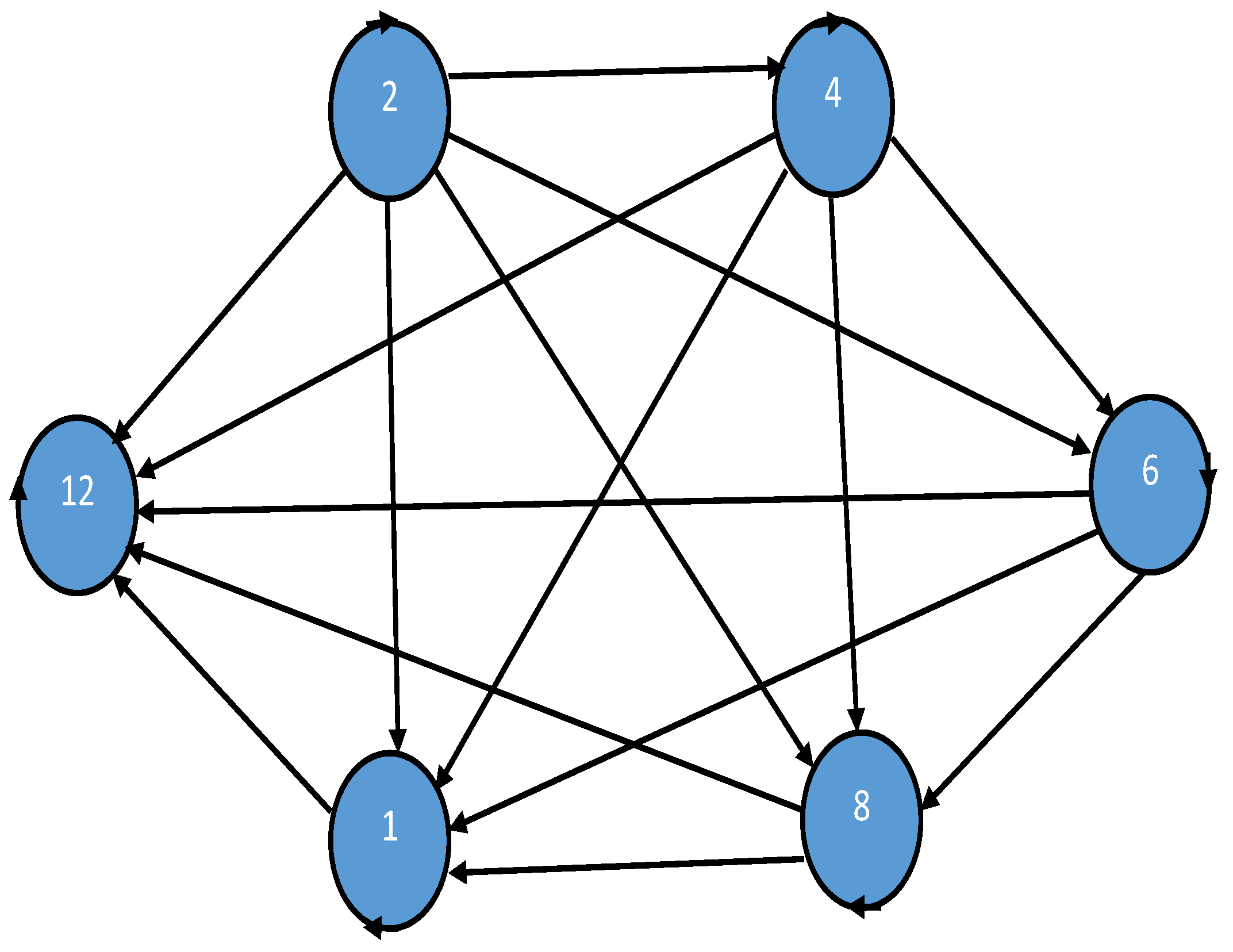
Example 3.

Let $Ł=\{2,4,6,8\}$, ${Ł}^{*}=\{1,6,8,12\}$, and the function $d_{\mathsf{\Theta }}:Ł\times {Ł}^{*}\to {\mathbb{R}}^{+}$ is defined as

$$d_{\mathsf{\Theta }}(\partial ,ð)=\left\{\begin{array}{c}0, if \partial =ð\\ min\{\partial ,ð\},otherwise,\end{array}\right.$$

for all $\partial \in Ł$, $ð\in {Ł}^{*}$ and equipped with graph $\mathsf{\Theta }.$ The graph $\mathsf{\Theta }=\left(V\right(\mathsf{\Theta }),E(\mathsf{\Theta }\left)\right)$, having the set of vertices

$$V\left(\mathsf{\Theta }\right)=Ł\cup {Ł}^{*}=\{1,2,4,6,8,12\},$$

and the set of edges obtained from the vertex set $V\left(\mathsf{\Theta }\right)$, is obtained as

$$E\left(\mathsf{\Theta }\right)=▵\cup \left\{\begin{array}{c}(2,4),(2,6),(2,8),(2,1),(2,12),\\ (4,6),(4,8),(4,1),(4,12),(6,8),\\ (6,1),(6,12),(8,1),(8,12),(1,12)\end{array}\right\}.$$

See Figure 2 for further exposition. It is simple to confirm that $(Ł,{Ł}^{*},d_{\mathsf{\Theta }})$ is a graphical bipolar b-$\mathtt{MS}$ with $b=2$.

Now, we define a $\mathtt{CoVM}$

$$f:(Ł,{Ł}^{*},d_{\mathsf{\Theta }})\rightrightarrows (Ł,{Ł}^{*},d_{\mathsf{\Theta }}),$$

with $f\left(Ł\right)\subseteq Ł$ and $f\left({Ł}^{*}\right)\subseteq {Ł}^{*},$ where

$$f\partial =6,if\partial \in \{4,6\},andfð=6,ifð\in \{1,12\},$$

for all $\partial \in Ł$ and $ð\in {Ł}^{*}.$

Furthermore, if $\partial =4$ and $ð=12,$ we have the following

$$\begin{array}{ccc}\hfill d_{\mathsf{\Theta }}(f4,f12)& \le & \frac{\gamma }{b^2}{d}_{\mathsf{\Theta }}(4,12)\hfill \\ \hfill d_{\mathsf{\Theta }}(6,6)& \le & \frac{\gamma }{b^2}{d}_{\mathsf{\Theta }}(4,12)\hfill \\ \hfill 0& \le & \frac{\gamma }{b^2}\left(4\right).\hfill \end{array}$$

Again, if $\partial =4$ and $ð=1,$ we infer

$$\begin{array}{ccc}\hfill d_{\mathsf{\Theta }}(f4,f1)& \le & \frac{\gamma }{b^2}{d}_{\mathsf{\Theta }}(4,1)\hfill \\ \hfill d_{\mathsf{\Theta }}(6,6)& \le & \frac{\gamma }{b^2}{d}_{\mathsf{\Theta }}(4,1)\hfill \\ \hfill 0& \le & \frac{\gamma }{b^2}\left(1\right),\hfill \end{array}$$

proving that f is a ${\mathsf{\Theta }}_b-$contraction with $b=2$ and $\gamma =1,$ where $0<\gamma <b.$ A simple computation leads us to obtain $\frac{\gamma }{b^2}=\frac{1}{4}$. This shows that all the assertions of the Theorem 1 are met, and f concedes a fixed point for all $\partial \in Ł$ and $ð\in {Ł}^{*},$ which is $6\in Ł\cap {Ł}^{*}.$

Below, we will prove a similar result for $\mathtt{CnVMs}$.

Definition 12.

Let Θ be a graph containing all the loops associated with graphical bipolar b-$\mathtt{MS}$ $(Ł,{Ł}^{*},d_{\mathsf{\Theta }}).$ A $\mathtt{CnVM}$ $f:$ $(Ł,{Ł}^{*},d_{\mathsf{\Theta }})\rightleftarrows (Ł,{Ł}^{*},d_{\mathsf{\Theta }})$ is said to be a ${\mathsf{\Theta }}_b^{*}-$contraction (on $Ł\cup {Ł}^{*})$ on a graphical bipolar b-$\mathtt{MS}$ $(Ł,{Ł}^{*},d_{\mathsf{\Theta }})$ if the following axioms are upheld:

(i) 

For $(\partial ,ð)\in E\left(\mathsf{\Theta }\right)$, we have

$$(f\partial ,fð)\in E\left(\mathsf{\Theta }\right),forall\partial \in Ł,ð\in {Ł}^{*}.$$

(7)

(ii) 

There exists $0<\gamma <b$ for all $\partial \in Ł,$ and $ð\in {Ł}^{*}$ with $(\partial ,ð)\in E\left(\mathsf{\Theta }\right)$ implies

$$d_{\mathsf{\Theta }}(f\partial ,fð)\le \frac{\gamma }{b^2}{d}_{\mathsf{\Theta }}(ð,\partial ).$$

(8)

Theorem 3.

Let $f:$ $(Ł,{Ł}^{*},d_{\mathsf{\Theta }})\rightleftarrows (Ł,{Ł}^{*},d_{\mathsf{\Theta }})$ be a graphical ${\mathsf{\Theta }}_b^{*}-$contraction on a $\mathsf{\Theta }-$complete graphical bipolar b-$\mathtt{MS}$ $(Ł,{Ł}^{*},d_{\mathsf{\Theta }})$ if the following conditions hold:

(i) 

Θ exhibits the property $\left(P^{*}\right)$.

(ii) 

There exists ${\partial }_0\in Ł,$ and ${ð}_0\in {Ł}^{*}$ with $(f{\partial }_0,f{ð}_0)\in {\left[({\partial }_0,{ð}_0)\right]}_{\mathsf{\Theta }}^l$ for some $l\in \mathbb{N}.$

Then, there exists $\kappa \in Ł\cap {Ł}^{*}$ such that $f-P_{b}S$ $({\partial }_m,{ð}_m)$ with the initial value ${\partial }_0\in Ł,$ ${ð}_0\in {Ł}^{*}$ is ${\mathsf{\Theta }}^{*}-TWC$ and bi-converges to both $\kappa$ and $f\kappa$.

Proof. 

Let ${\partial }_0\in Ł$ such that $(f{\partial }_0,f{ð}_0)\in {\left[({\partial }_0,{ð}_0)\right]}_{\mathsf{\Theta }}^l$ for some $l\in \mathbb{N}.$ By taking ${\partial }_0\in Ł$ as the initial values of $f-P_{b}S$ $({\partial }_m,{ð}_m),$ there exists a path ${\left\{({\partial }_j,{ð}_j)\right\}}_{j=0}^l,$ such that ${ð}_n=f{\partial }_n$ and ${\partial }_{n+1}=f{ð}_n$ where $({\partial }_j,{ð}_j)\in E\left(\mathsf{\Theta }\right)$ for $j=0,1,\dots ,l.$ By using (7), we assert that $(f{\partial }_{j-1},f{ð}_j)\in E\left(\mathsf{\Theta }\right)$ for $j=1,\dots ,l.$ This implies that ${\left\{(f{\partial }_j,f{ð}_j)\right\}}_{j=0}^l$ is a path from ${\partial }_2=f^2{\partial }_1=f^3{\partial }_0$ to ${ð}_2=f^2{ð}_1=f^3{ð}_0$ having length l such that $({\partial }_2,{ð}_2)\in {\left[({\partial }_1,{ð}_1)\right]}_{\mathsf{\Theta }}^l.$ Continuing this procedure, we conclude that ${\left\{(f^m{\partial }_j,f^m{ð}_j)\right\}}_{j=0}^l$ is a path from $(f^m{\partial }_0,f^m{ð}_0)=({\partial }_m,{ð}_m)$ to $(f^{m+l}{\partial }_0,f^{m+l}{ð}_0)=({\partial }_{m+l},{ð}_{m+l})$ of length l and hence $({\partial }_{m+1},{ð}_{m+1})\in$ ${\left[({\partial }_m,{ð}_m)\right]}_{\mathsf{\Theta }}^l$ for all $m\in$ $\mathbb{N}.$ This confirms that $({\partial }_m,{ð}_m)$ is a ${\mathsf{\Theta }}^{*}-TWC$ $BC$, which shows that

$$(f^m{\partial }_j,f^m{ð}_j)\in E\left(\mathsf{\Theta }\right)\mathrm{for}j=1,2\dots ,l\mathrm{and}m\in \mathbb{N}.$$

Imposing inequality (8), we infer

$$\begin{array}{ccc}\hfill d_{\mathsf{\Theta }}(f^m{\partial }_j,f^m{ð}_j)& \le & \frac{\gamma }{b^2}{d}_{\mathsf{\Theta }}(f^{m-1}{ð}_j,f^m{\partial }_j)\hfill \\ & \le & \frac{{\gamma }^2}{b^4}{d}_{\mathsf{\Theta }}(f^{m-1}{ð}_j,f^{m-1}{\partial }_j)\hfill \\ & =& \frac{{\gamma }^2}{b^4}{d}_{\mathsf{\Theta }}(f^{m-1}{\partial }_j,f^{m-1}{ð}_j).\hfill \end{array}$$

Continuing the same approach, we arrive at the conclusion that

$$d_{\mathsf{\Theta }}(f^m{\partial }_j,f^m{ð}_j)\le \frac{{\gamma }^{2m}}{b^{4m}}{d}_{\mathsf{\Theta }}({\partial }_j,{ð}_j).$$

Since the $BC$ $({\partial }_n,{ð}_n)$ is a ${\mathsf{\Theta }}^{*}-TWC$ $BC$, it is imperative to prove that $({\partial }_n,{ð}_n)$ is Cauchy $BC$ in graphical bipolar b-$\mathtt{MS}$ $(Ł,{Ł}^{*},d_{\mathsf{\Theta }})$. For every positive integer n and m, we proceed as follows:

$$\begin{array}{ccc}\hfill d_{\mathsf{\Theta }}({\partial }_n,{ð}_n)& =& d_{\mathsf{\Theta }}(f\left({ð}_{n-1}\right),f\left({\partial }_n\right))\hfill \\ & \le & \frac{\gamma }{b^2}{d}_{\mathsf{\Theta }}({\partial }_n,{ð}_{n-1})\hfill \\ & \le & \frac{{\gamma }^2}{b^4}{d}_{\mathsf{\Theta }}({\partial }_{n-1},{ð}_{n-1})\hfill \\ & & ⋮\hfill \\ & \le & \frac{{\gamma }^{2n}}{b^{4n}}{d}_{\mathsf{\Theta }}({\partial }_0,{ð}_0),\hfill \end{array}$$

Furthermore,

$$\begin{array}{ccc}\hfill d_{\mathsf{\Theta }}({\partial }_n,{ð}_{n+1})& =& d_{\mathsf{\Theta }}(f\left({\partial }_{n-1}\right),f\left({ð}_n\right))\hfill \\ & \le & \frac{\gamma }{b^2}{d}_{\mathsf{\Theta }}({\partial }_{n-1},{ð}_n)\hfill \\ & & ⋮\hfill \\ & \le & \frac{{\gamma }^{2n}}{b^{4n}}{d}_{\mathsf{\Theta }}({\partial }_0,{ð}_1).\hfill \end{array}$$

Now, for $m\ge n,$ we obtain

$$\begin{array}{ccc}\hfill d_{\mathsf{\Theta }}(f{\partial }_m,f{ð}_n)& \le & b[d_{\mathsf{\Theta }}(f{\partial }_m,f{ð}_{n+1})+d_{\mathsf{\Theta }}(f{\partial }_n,f{ð}_{n+1})+d_{\mathsf{\Theta }}(f{\partial }_n,f{ð}_n)]\hfill \\ & \le & b[d_{\mathsf{\Theta }}(f{\partial }_m,f{ð}_{n+1})+\frac{{\gamma }^n}{b^{4n}}{d}_{\mathsf{\Theta }}({\partial }_0,{ð}_1)+\frac{{\gamma }^n}{b^{4n}}{d}_{\mathsf{\Theta }}({\partial }_0,{ð}_0)]\hfill \\ & \le & b{d}_{\mathsf{\Theta }}(f{\partial }_m,f{ð}_{n+1})+\frac{{\gamma }^n}{b^{4n-1}}[d_{\mathsf{\Theta }}({\partial }_0,{ð}_1)+d_{\mathsf{\Theta }}({\partial }_0,{ð}_0)].\hfill \end{array}$$

(9)

Moreover,

$$\begin{array}{ccc}\hfill d_{\mathsf{\Theta }}(f{\partial }_m,f{ð}_{n+1})& \le & b[d_{\mathsf{\Theta }}(f{\partial }_m,f{ð}_{n+2})+d_{\mathsf{\Theta }}(f{\partial }_{n+1},f{ð}_{n+2})+d_{\mathsf{\Theta }}(f{\partial }_{n+1},f{ð}_{n+1})]\hfill \\ & \le & b[d_{\mathsf{\Theta }}(f{\partial }_m,f{ð}_{n+2})+\frac{{\gamma }^{2(n+1)}}{b^{4(n+1)}}{d}_{\mathsf{\Theta }}({\partial }_0,{ð}_1)+\frac{{\gamma }^{2(n+1)}}{b^{4(n+1)}}{d}_{\mathsf{\Theta }}({\partial }_0,{ð}_0)]\hfill \\ & \le & b{d}_{\mathsf{\Theta }}(f{\partial }_m,f{ð}_{n+2})+\frac{{\gamma }^{2(n+1)}}{b^{4(n+1)-1}}[d_{\mathsf{\Theta }}({\partial }_0,{ð}_1)+d_{\mathsf{\Theta }}({\partial }_0,{ð}_0)].\hfill \end{array}$$

(10)

Similarly, we obtain

$$\begin{array}{ccc}\hfill d_{\mathsf{\Theta }}(f{\partial }_m,f{ð}_{m-1})& \le & b[d_{\mathsf{\Theta }}(f{\partial }_m,f{ð}_m)+d_{\mathsf{\Theta }}(f{\partial }_{m-1},f{ð}_m)+d_{\mathsf{\Theta }}(f{\partial }_{m-1},f{ð}_{m-1})]\hfill \\ & \le & b[d_{\mathsf{\Theta }}(f{\partial }_m,f{ð}_m)+\frac{{\gamma }^{2(m-1)}}{b^{4(m-1)}}{d}_{\mathsf{\Theta }}({\partial }_0,{ð}_1)+\frac{{\gamma }^{2(m-1)}}{b^{4(m-1)}}{d}_{\mathsf{\Theta }}({\partial }_0,{ð}_0)]\hfill \\ & \le & b{d}_{\mathsf{\Theta }}(f{\partial }_m,f{ð}_m)+\frac{{\gamma }^{2(m-1)}}{b^{4(m-1)-1}}[d_{\mathsf{\Theta }}({\partial }_0,{ð}_1)+d_{\mathsf{\Theta }}({\partial }_0,{ð}_0)].\hfill \end{array}$$

(11)

From the observations (9)–(11), if we set $M=d_{\mathsf{\Theta }}({\partial }_0,{ð}_1)+d_{\mathsf{\Theta }}({\partial }_0,{ð}_0)$, we arrive at

$$\begin{array}{ccc}\hfill d_{\mathsf{\Theta }}(f{\partial }_m,f{ð}_n)& \le & b{d}_{\mathsf{\Theta }}(f{\partial }_m,f{ð}_{n+1})+\frac{{\gamma }^{2n}}{b^{4n-1}}M\hfill \\ & \le & b^2{d}_{\mathsf{\Theta }}(f{\partial }_m,f{ð}_{n+2})+\frac{{\gamma }^{2n}}{b^{4n-1}}M+\frac{{\gamma }^{2(n+1)}}{b^{4(n+1)-1}}M\hfill \\ & & ⋮\hfill \\ & \le & b^{m-n}{d}_{\mathsf{\Theta }}(f{\partial }_m,f{ð}_m)+\frac{{\gamma }^{2n}}{b^{4n-1}}M+\frac{{\gamma }^{2(n+1)}}{b^{4(n+1)-1}}M+\dots +\frac{{\gamma }^{2(m-1)}}{b^{4(m-1)-1}}M\hfill \\ & \le & b^{m-n}\frac{{\gamma }^{2m}}{b^{4m}}M+\frac{{\gamma }^{2n}}{b^{4n-1}}M+\frac{{\gamma }^{2(n+1)}}{b^{4(n+1)-1}}M+\dots +\frac{{\gamma }^{2(m-1)}}{b^{4(m-1)-1}}M\hfill \\ & \le & \frac{{\gamma }^{2n}}{b^{4n-1}}M+\frac{{\gamma }^{2(n+1)}}{b^{4(n+1)-1}}M+\dots +\frac{{\gamma }^{2(m-1)}}{b^{4(m-1)-1}}M+\frac{{\gamma }^{2m}}{b^{3m+n}}M\hfill \\ & \le & \frac{1}{b}[{(\frac{{\gamma }^2}{b^4})}^{n}M+{(\frac{{\gamma }^2}{b^4})}^{n+1}M+\dots +{(\frac{{\gamma }^2}{b^4})}^{m-1}M+{(\frac{{\gamma }^2}{b^4})}^{m}M]\hfill \\ & \le & \frac{1}{b}\left[\frac{{(\frac{{\gamma }^2}{b^4})}^{n}M}{1-(\frac{{\gamma }^2}{b^4})}\to 0\right]\to 0,\hfill \end{array}$$

which shows that $({\partial }_n,{ð}_n)$ is a Cauchy $BC$. Since $(Ł,{Ł}^{*},d_{\mathsf{\Theta }})$ is a $\mathsf{\Theta }-$complete graphical bipolar b-$\mathtt{MS}$, then $BC$ $({\partial }_n,{ð}_n)$ is bi-convergent to $\kappa$ in $Ł\cap {Ł}^{*}$ and from $\left(i\right)$ there exists some $\kappa \in Ł\cap {Ł}^{*},$ $n_0\in \mathbb{N}$ such that $\left(({\partial }_n,{ð}_n),\kappa \right)\in E\left(\mathsf{\Theta }\right)$ and $\left(\kappa ,({\partial }_n,{ð}_n)\right)\in E\left(\mathsf{\Theta }\right)$ for all $n>n_0$ and

$$\underset{n\to \infty }{lim}{d}_{\mathsf{\Theta }}\left(({\partial }_n,{ð}_n),\kappa \right)=0,$$

which confirms that $BC$ $({\partial }_n,{ð}_n)$ is bi-convergent to $\kappa .$ If $\left(({\partial }_n,{ð}_n),\kappa \right)\in E\left(\mathsf{\Theta }\right)$, then by using (8)

$$\begin{array}{ccc}\hfill d_{\mathsf{\Theta }}\left(({\partial }_{n+1},{ð}_{n+1}),\kappa \right)& =& d_{\mathsf{\Theta }}\left((f{ð}_n,f{\partial }_{n+1}),f\kappa \right)\hfill \\ & \le & \frac{\gamma }{b^2}{d}_{\mathsf{\Theta }}\left(({\partial }_{n+1},{ð}_n),\kappa \right)\hfill \\ & \le & \frac{{\gamma }^2}{b^4}{d}_{\mathsf{\Theta }}\left(({\partial }_n,{ð}_n),\kappa \right)\hfill \end{array}$$

for all $n>n_0,$ which shows that

$$\underset{n\to \infty }{lim}{d}_{\mathsf{\Theta }}\left(({\partial }_{n+1},{ð}_{n+1}),\kappa \right)=0.$$

If $\left(\kappa ,({\partial }_n,{ð}_n)\right)\in E\left(\mathsf{\Theta }\right),$ a similar argument to that we used above,

$$\underset{n\to \infty }{lim}{d}_{\mathsf{\Theta }}\left(\kappa ,(f{\partial }_{n+1},f{ð}_{n+1})\right)=0.$$

Hence, $BC$ $({\partial }_n,{ð}_n)$ is bi-convergent to $\kappa$ and $f\kappa .$ □

To demonstrate that mapping f has a fixed point, we employ the attribute $\left(P^{*}\right).$

Theorem 4.

If all the hypotheses are retained in Theorem 3 and we further suppose that the quadruple $(Ł,{Ł}^{*},d_{\mathsf{\Theta }},f)$ fulfills the property $\left(P^{*}\right),$ then f concedes a fixed point.

Proof. 

From the Theorem 3, we find that $f-P_{b}S$ $({\partial }_n,{ð}_n)$ with the initial values ${\partial }_0\in Ł$ bi-converges to both $\kappa$ and $f\kappa .$ Since $\kappa \in Ł\cap {Ł}^{*}$ and $f\kappa \in f(Ł\cap {Ł}^{*}),$ by hypothesis, we obtain $\kappa =f\kappa$ and f concedes a fixed point. □

Below, we will discuss an example related to Theorem 3 with different cases.

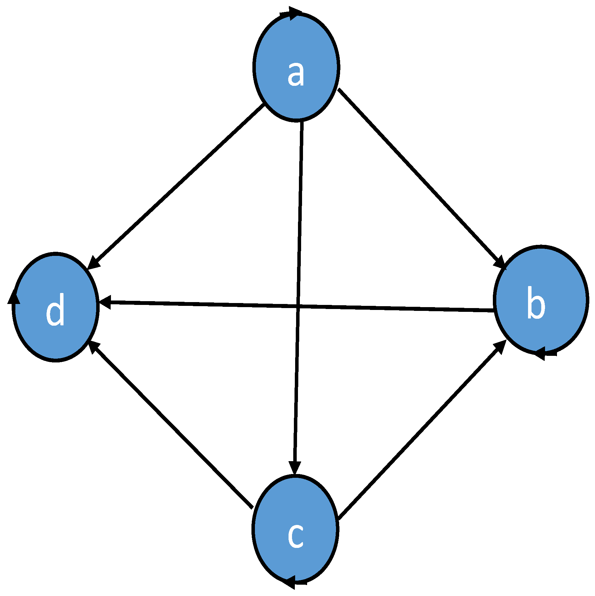
Example 4.

Let $Ł=\{a,b,c\}$, ${Ł}^{*}=\{b,c,d\}$ and $d_{\mathsf{\Theta }}:Ł\times {Ł}^{*}\to {\mathbb{R}}^{+}$ be defined as

$$\begin{array}{|ccccc|}\hline \hfill d_{\mathsf{\Theta }}& a& b\hfill & c& d\\ \hfill a& 0& 1\hfill & 2& 4\\ \hfill b& 1& 0\hfill & 1& 2\\ \hfill c& 2& 1\hfill & 0& 1\\ \hfill d& 4& 2\hfill & 1& 0\\ \hline\end{array}$$

for all $\partial \in Ł$ and $ð\in {Ł}^{*}.$ For $b=\frac{4}{3}>1$, it is simple to observe that $(Ł,{Ł}^{*},d_{\mathsf{\Theta }})$ is graphical bipolar $\mathtt{MS}$ with the vertex set $V\left(\mathsf{\Theta }\right)=Ł\cup {Ł}^{*}$ and edge set $E\left(\mathsf{\Theta }\right)=\left\{\right(a,b),(a,c),(a,d),(c,b),(b,d),(c,d\left)\right\}$, as shown in Figure 3.

We define a $\mathtt{CnVM}$ using the following:

$$f:(Ł,{Ł}^{*},d_{\mathsf{\Theta }})\rightleftarrows (Ł,{Ł}^{*},d_{\mathsf{\Theta }}),$$

with $f\left(Ł\right)\subseteq {Ł}^{*}$, $f\left({Ł}^{*}\right)\subseteq Ł$ such that

$$f\partial =\left\{\begin{array}{c}c,if\partial =a,\\ d,if\partial =b,\end{array}\right.$$

and

$$fð=\left\{\begin{array}{c}b,ifð=b,\\ c,ifð=d,\end{array}\right.$$

for all $\partial \in Ł$, $ð\in {Ł}^{*}.$

The cases below are examined while assuming that $\gamma =\frac{11}{10}$:

Case (i): When $\partial =a$ and $ð=d$, then

$$\begin{array}{ccc}\hfill d_{\mathsf{\Theta }}(fa,fd)& \le & \frac{\gamma }{b^2}{d}_{\mathsf{\Theta }}(b,d)\hfill \\ \hfill d_{\mathsf{\Theta }}(c,c)& \le & \frac{\gamma }{b^2}{d}_{\mathsf{\Theta }}(b,d)\hfill \\ \hfill 0& \le & \frac{\gamma }{b^2}\left(2\right).\hfill \end{array}$$

Evidently, the case holds for $\gamma =\frac{11}{10}$ and $b=\frac{4}{3}$.

Case (ii): For $\partial =b$ and $ð=d$,

$$\begin{array}{ccc}\hfill d_{\mathsf{\Theta }}(fb,fd)& \le & \frac{\gamma }{b^2}{d}_{\mathsf{\Theta }}(b,d)\hfill \\ \hfill d_{\mathsf{\Theta }}(d,c)& \le & \frac{\gamma }{b^2}{d}_{\mathsf{\Theta }}(b,d)\hfill \\ \hfill 1& \le & \frac{\gamma }{b^2}\left(2\right).\hfill \end{array}$$

Hence, ${\mathsf{\Theta }}_b^{*}-$contraction is satisfied for $b=\frac{4}{3}$ and $\gamma =\frac{11}{10},$ where $0<\gamma <b.$ After simple calculation, we obtain $\frac{\gamma }{b^2}=0.61875<1$. This suggests that all the requirements of Theorem 3 are satisfied, and f concedes a fixed point for all $\partial \in Ł$ and $ð\in {Ł}^{*},$ which is $b\in Ł\cap {Ł}^{*}.$

Similarly, we can continue Example 3 related to Theorem 1 with $\mathtt{CnVM}$.

Example 5.

If we take all the terms and conditions of Example 3 and define a $\mathtt{CnVM}$

$$f:(Ł,{Ł}^{*},d_{\mathsf{\Theta }})\rightleftarrows (Ł,{Ł}^{*},d_{\mathsf{\Theta }}),$$

with $f\left(Ł\right)\subseteq {Ł}^{*}$ and $f\left({Ł}^{*}\right)\subseteq Ł$ such that

$$f\partial =1,if\partial =6,andfð=8,ifð\in \{8,12\},$$

for all $\partial \in Ł$ and ${Ł}^{*}\in {Ł}^{*}.$

For $\partial =6$ and $ð=12,$ then

$$\begin{array}{ccc}\hfill d_{\mathsf{\Theta }}(f6,f12)& \le & \frac{\gamma }{b^2}{d}_{\mathsf{\Theta }}(6,12)\hfill \\ \hfill d_{\mathsf{\Theta }}(1,8)& \le & \frac{\gamma }{b^2}{d}_{\mathsf{\Theta }}(6,12)\hfill \\ \hfill 1& \le & \frac{\gamma }{b^2}\left(6\right),\hfill \end{array}$$

which is true for $b=2$ and $\gamma =1$.

Hence, ${\mathsf{\Theta }}_b^{*}-$contraction is satisfied for $b=2$ and $\gamma =1,$ where $0<\gamma <b.$ With routine calculations, we obtain $\frac{\gamma }{b^2}=\frac{1}{4},$ showing that all the requirements of Theorem 3 are met, and f concedes a fixed point for all $\partial \in Ł$ and $ð\in {Ł}^{*},$ which is $8\in Ł\cap {Ł}^{*}.$

Remark 3.

It is important to note that all of the conclusions presented in this article apply equally to symmetric graphs, or graphs in which edge symmetry exists.

5. Conclusions

Metric spaces and their various generalizations allow us to consider the distances between points in a set, either classically or non-classically. However, in some situations, distances might occur between components of two distinct sets compared to between points of a single set. Distances among the same type of points are either indefinite or unclear in some circumstances due to a lack of data. Illustrations of these distances abound in mathematics and science. Some examples include distance within lines and points in a Euclidean space, suitability measurement of habitats to species, an affinity across a group of students, and a set of duties, etc. We formalize such distances as the graphical bipolar b-metric but only examine them isometrically without deeply delving into their topological aspects. We begin by offering basic definitions and examples of graphical bipolar b-$\mathtt{MS}$, then explain maps and bi-sequences, investigate the completeness, explore some related features, and conclude with convergence results, employing covariant and contravariant mapping contractions in the form of graphs.

With this aim, we instigate a novel notion, termed graphical bipolar b-metric spaces, which combines graphical analysis and fixed-point theory. We propound fixed-point results using covariant and contravariant mapping contractions within the context of graphical bipolar b-metric spaces, a novel study within the field of graphical metric spaces, considering the symmetry of the edges of the underlying graph. These results are the first of their kind in the current state of the art. Illustrative examples with appropriate graphs are provided to demonstrate the findings. These examples help to improve the comprehension and implementation of the concepts that have been developed.

We offer the following open questions for future developments of this study:

▸

Can the proposed convergence theorems in this study be generalized to multi-valued mappings?

▸

Is it possible to use $\mathtt{CnVM}$ and $\mathtt{CoVM}$ to obtain the fixed points for Reich-type contractions in a graph setting?