Groups of Coordinate Transformations between Accelerated Frames

Abstract

The analysis of the present paper reveals that, besides the relativistic symmetry expressed by the Lorentz group of coordinate transformations which leave invariant the Minkowski metric of space-time of inertial frames, there exists one more relativistic symmetry expressed by a group of coordinate transformations leaving invariant the space-time metric of the frames with a constant proper-acceleration. It is remarkable that, in the flat space-time, only those two relativistic symmetries, corresponding to groups of continuous transformations leaving invariant the metric of space-time of extended rigid reference frames, exist. Therefore, the new relativistic symmetry should be considered on an equal footing with the Lorentz symmetry. The groups of transformations leaving invariant the metric of the space-time of constant proper-acceleration are determined using the Lie group analysis, supplemented by the requirement that the group include transformations to or from an inertial to an accelerated frame. Two-parameter groups of two-dimensional (1 + 1), three-dimensional (2 + 1), and four-dimensional (3 + 1) transformations, with the group parameters related to the ratio of accelerations of the frames and the relative velocity of the frame space origins at the initial moment, can be considered as counterparts of the Lorentz group of corresponding dimensions. Defining the form of the interval and the groups of coordinate transformations satisfying the relativity principle paves the way to defining the invariant forms of the laws of dynamics and electrodynamics in accelerated frames. Thus, the problem of extending the relativity principle from inertial to uniformly accelerated frames has been resolved without use of the equivalence principle and/or the general relativity equations. As an application of the transformations to purely kinematic phenomena, the problem of differential aging between accelerated twins is treated.

1. Introduction

Lorentz symmetry is arguably the most fundamental symmetry in physics, at least in its modern conception. It is theoretically and experimentally confirmed that fundamental physical laws are Lorentz-covariant among inertial frames, namely, the form of a physical law is invariant under the Lorentz group of space-time transformations. Nevertheless, one cannot be content with the fact that the relativity principle, from which the special relativity theory (SRT) stems, is valid only for the specific choice of reference system. In general, the relativity principle asserts that the equations describing the laws of physics have the same form in all admissible frames of reference. Criteria for a class of reference systems to be admissible in the context of the relativity principle is a separate issue, that should be discussed, but that general formulation of the relativity principle implies that the area of applicability of the relativity principle could be extended to non-inertial reference frames.

The problem of extending the relativity principle to non-inertial accelerated frames was first formulated by A. Einstein in his 1907 paper [1]: (throughout the Introduction, quotations from original works are marked by italic): So far we have applied the principle of relativity, i.e., the assumption that the physical laws are independent of the state of motion of the reference system, only to nonaccelerated reference systems. Is it conceivable that the principle of relativity also holds for systems which accelerate relative to each other? While this is not the place for a detailed discussion of this question, it will occur to anybody who has been following the applications of the principle of relativity. In the part of the paper [1] following the question, Einstein formulates the equivalence principle as follows …we shall therefore assume the complete physical equivalence of a gravitational field and a corresponding acceleration of the reference system. This assumption extends the principle of relativity to the uniformly accelerated translational motion of the reference system. The heuristic value of this assumption rests on the fact that it permits the replacement of a homogeneous gravitational field by a uniformly accelerated reference system, the latter case being to some extent accessible to theoretical treatment. As a matter of fact, the above cited Einstein’s interpretation of the equivalence principle includes two issues: The first one is the extension of the relativity principle to accelerated frames and the second one is gravity. Those two issues are conceptually different and, in general, one could not expect that they should be realted to each other. The second concept, gravity, had been further developed to eventually arrive at the General Relativity Theory (GRT). As it is formulated in [2], by identifying accelerated reference systems to the gravitational field, A. Einstein came to perceive the metric space-time tensor as the principal characteristic of the gravitational field. This way, A. Einstein arrived at the necessity of introducing Riemannian space since he considered the metric tensor of this space to describe gravity.

The first concept, the relativity principle for accelerated frames, had not been further developed and remained related to the equivalence principle. At the first stages of developing the GRT, the equivalence principle was treated as part of the conceptual framework of the GRT. However, in the modern view, the assessment of the role of the equivalence principle is more controversial. Most authors admit its validity, with the reservation that the equivalence principle applies only locally, while some others deny its validity and consider that the equivalence principle, at least in the formulation of Einstein’s 1907 paper, has nothing to do with the essence of GRT. According to V. A. Fock [2], the essence of GRT is the unity of the Riemannian metric and gravity and the equivalence principle reduces to the statement that it is possible to introduce locally geodesic (“freely falling”) frame of reference such that the Galilean space is defined in an infinitesimal region of space. However, in Fock’s opinion, this in no way justifies the original formulation of the principle about the equivalence of fields of acceleration and gravity. Therefore, it is inconsistent to interpret the equivalence principle as a “General Principle of Relativity” and even the name GRT given to the theory of gravitation is a misnomer. The same is asserted by J. L. Synge [3]: The possibility to introduce locally geodesic frame of reference only defines the signature of the space-time metric, it is important, but hardly a Principle and In Einstein’s theory, either there is a gravitational field or there is none, according as the Riemann tensor does not or does vanish. This is an absolute property; it has nothing to do with any observer’s world-line. In any case, the opinion, that the problem of extending the relativity principle to accelerated frames is resolved by the equivalence principle and GRT is unjustified.

As a matter of fact, the formulation of the problem of extending the relativity principle from inertial frames to accelerated frames in Einstein’s paper [1] suggests that the relativity principle, similar to that for inertial systems, is implied. This includes defining transformations of space and time variables between accelerated frames as counterparts of the Lorentz transformations and formulating physical laws in the form invariant under the transformations between accelerated frames. In general, there are no grounds for the issue of gravity to be involved in that problem; it became involved only due to putting forward the equivalence principle and interpreting it in the context of the principle of relativity by A. Einstein. In the present study, the problem of extending the relativity principle to accelerated frames is tackled without any considerations related to gravity—in particular, neither the equivalence principle nor the general relativity equations are used.

To make the concept of the relativity principle precise, let us start from the formulation of the principle of relativity by V. A. Fock ([2], Section ${49}^{*}$): In its most general form the principle of relativity states the equivalence of the coordinate systems (or frames of reference) that belong to a certain class and are related by transformations of the form $x_{\alpha }^{\prime }=f_{\alpha }\left(x_0,x_1,x_2,x_3\right)$ which may be stated more briefly as $x^{\prime }=f\left(x\right)$. …Two reference frames (x) and ($x^{\prime }$) may be called physically equivalent if phenomena proceed in the same way in them. This means that if a possible process is described in the coordinates (x) by the functions ${\varphi }_1\left(x\right),{\varphi }_2\left(x\right),\dots ,{\varphi }_n\left(x\right)$ then there is another possible process which is describable by the same functions ${\varphi }_1\left(x^{\prime }\right),{\varphi }_2\left(x^{\prime }\right),\dots ,{\varphi }_n\left(x^{\prime }\right)$ in the coordinates ($x^{\prime }$). …Thus, the relativity principle is a statement concerning the existence of corresponding processes in a set of reference frames of a certain class; the systems of this class are then accepted as equivalent. …the very notion of a ’principle of relativity’ becomes well defined only when a definite class of frames of reference has been singled out. In the usual theory of relativity this class is that of inertial systems.

The transformations between the reference frames should satisfy a number of physical requirements, such as associativity, reciprocity, and so on, which are all covered by the requirement that the transformations form a group. As it is stated in [2], The uniformity of space and time manifests itself in the existence of a group of transformations that leave invariant the four-dimensional distance or interval between two points. It is indicated in [2] that the coefficients in the expression for the squared infinitesimal distance, the components of the metric tensor $g_{ik}$, must be included among the functions ${\varphi }_{\alpha }\left(x\right)$ describing a physical process (’functions of state’). Thus, if $g_{ik}$ are functions of coordinates, the transformations should leave the mathematical form of those functions unchanged, which means that the interval should also be form-invariant. The relativity principle and the existence of a group of transformations are closely related. The existence of a group of coordinate-time transformations signifies that there exists an infinite set of equivalent reference frames related to the transformations, which is necessary for the relativity principle to be well defined. The relativity principle also implies that physical equations for the functions of state ${\varphi }_{\alpha }\left(x\right)$ or $\varphi \left(x^{\prime }\right)$, in all the reference frames related by the transformations should be identical, or, in other words, the equations should be invariant under the group transformations. It follows from the invariance of the equations that any phenomenon that proceeds in equivalent reference systems under identical conditions will yield identical results, i.e., the relativity principle is satisfied. In somewhat different terms, the existence of a group of transformations leaving the interval between two points invariant indicates the existence of the corresponding symmetry of space-time which, in the context of the relativity principle, can be named a relativistic symmetry.

Thus, to extend the relativity principle to accelerated frames the following should be implemented. First, the class of reference frames, which represents a consistent generalization of the inertial frames of special relativity should be defined. Second, the expression for the interval should be defined. Evidently, defining the class of reference systems is intrinsically linked to defining the form of the interval. Third, a group of transformations that leave the interval invariant (form-invariant), should be determined. Implementing those tasks paves the way for defining the forms of physical laws satisfying the relativity principle. In that respect, the expression for the interval plays an important role because its form is directly related to the form taken by the basic laws of physics, viz, the law of motion of a free mass particle and the law of propagation of the light wave front.

The class of accelerated frames of reference should be defined such that it were a counterpart of the class of inertial frames of the special theory of relativity. It means that the frames extended in space, representing a continuum of observers, should be considered. It is necessary that the observers fixed in the accelerated frame could construct a single set of space coordinates and a single time coordinate for the whole frame, for which it is required that (i) any two events that are simultaneous for one observer should be simultaneous for all observers (synchronization of clocks is possible over all space); (ii) at each point the space separations between the observers are constant from the point of view of each observer (rigid frame). This definition of a frame imposes restrictions on the form of the interval between two points of space-time. To satisfy the requirements (i) and (ii), the components $g_{0\alpha }$ in the form $d{s}^2=g_{ik}d{x}^{I}d{x}^k$ ($i,k$ run from 0 to 3 and $\alpha$ runs from 1 to 3) should vanish, and all $g_{ik}$ should not depend on $x_0$ (on time) [4]. (Note that even though those properties are discussed in [4] as related to the gravitational field, in fact, the analysis deals only with the properties of the metric of space-time.) Assuming that the z-axis is distinguished by the acceleration direction while taking the symmetry arguments into account, we can use the metric of the form

$$d{s}^2=A\left(z\right)d{t}^2-B\left(z\right)d{z}^2-d{x}^2-d{y}^2$$

(1)

as a starting point for our analysis (in (1) and in what follows, a system of units in which the light speed $c=1$ is used).

According to the above discussion, defining the form of the interval for which the relativity principle can be valid is equivalent to defining the form that can be invariant under a continuous group of space-time transformations. In other terms, the criteria for a class of reference frames to be admissible in the context of the relativity principle is the existence of a group of continuous transformations that relate the coordinates of the frames of that class and leave the interval invariant. Thus, at this stage of the analysis, the task of defining the admissible classes of reference frames reduces to defining specific forms of the interval (1) which allow a group of coordinate transformations leaving it invariant. That task is implemented by applying the infinitesimal Lie group technique which defines both the admissible forms and the groups of invariance of the interval (1). Applying the method yields the determining equations for the infinitesimal group generators, and the analysis reveals that the determining equations cannot be solved for arbitrary functions $A\left(z\right)$ and $B\left(z\right)$. It is possible only for specific forms of those functions, so one is confronted with the group classification problem. The result is that, in flat space-time, a group of continuous space-time transformations leaving the metric (1) invariant exists only for two specific forms of (1). The first one is that of a Minkowski space-time $(x^{\prime },y^{\prime },z^{\prime },t^{\prime })$ with a metric

$$d{s}^2={\left(d{t}^{\prime }\right)}^2-{\left(d{z}^{\prime }\right)}^2-{\left(d{x}^{\prime }\right)}^2-{\left(d{y}^{\prime }\right)}^2$$

(2)

(Here and throughout the paper, letters with primes are related to the coordinates of points in a Minkowski space-time (or, equivalently, events in an inertial system).) The second form is

$$d{s}^2=u{\left(z\right)}^{2}d{t}^2-{\left(\frac{u^{\prime }\left(z\right)}{g}\right)}^{2}d{z}^2-d{x}^2-d{y}^2$$

(3)

where g is a real constant and $u\left(z\right)$ is an arbitrary real function restricted by the requirement of continuity.

That result is remarkable. It shows that in flat space-time, besides the relativistic symmetry expressed by the Lorentz group of transformations leaving the Minkowski interval (2) invariant, there exists one more (but only one) relativistic symmetry corresponding to the group of invariance of the interval (3). The interval (3) does not reduce to the Minkowski interval (2) for any choice of the function $u\left(z\right)$ and therefore this relativistic symmetry should be considered on equal footing with the Lorentz symmetry. In the context of the relativity principle, the existence of space-time symmetry means that physical laws should maintain their form under the symmetry group transformations, or, in other terms, be the same regardless of the frame of reference used for description of the processes governed by the laws. The form of physical laws invariant under that new symmetry can be deduced in the same way as it is done in the case of Lorentz symmetry, but it should also be defined to what class of reference frames the new symmetry corresponds.

The form of the interval (3) arises in the literature in the context of coordinate transformations between inertial and accelerated frames (e.g., [5,6,7,8,9,10,11,12,13,14,15]). Most of the analyses are based on the equivalence principle, according to which the metric in the uniformly accelerated coordinate system is the same as that of a uniform and constant gravitational field. Correspondingly, the form (1) is treated as a general form for the metric of a static homogeneous gravitational field parallel to the z-axis, which is related by the equivalence principle to the reference frame accelerated along the z-axis. Then the metric (3) is specified from (1) using the field equations of general relativity (see, e.g., [5,14]), which in an empty space-time reduce to

$$R_{\mu \nu }=0$$

(4)

where $R_{\mu \nu }$ is the Ricci tensor. Alternatively the metric (3) can be derived from (1) using the condition for the space time to be flat (e.g., [9])

$$R_{\beta \mu \nu }^{\alpha }=0$$

(5)

where $R_{\beta \mu \nu }^{\alpha }$ is the Riemann-Christoffel curvature tensor. The most general form of the transformations converting the interval (3) into the Minkowski interval (2) is as follows

$$z^{\prime }=-\frac{coshb}{g}+\frac{u\left(z\right)}{g}cosh(gt+b),t^{\prime }=-\frac{sinhb}{g}+\frac{u\left(z\right)}{g}sinh(gt+b)$$

(6)

where b is a real constant and it is assumed that one event is the space-time origin of both frames. Most of the analyses consider only the $b=0$ particular case of (6) which is

$$\begin{array}{c}{x}^{\prime }=x,y^{\prime }=y,\hfill \\ z^{\prime }=\frac{u\left(z\right)}{g}cosh\left(gt\right)-\frac{1}{g},t^{\prime }=\frac{u\left(z\right)}{g}sinhgt\hfill \end{array}$$

(7)

It follows from equations (6) that the world-line of an observer fixed in the frame with the metric (3) represents a hyperbola in the inertial frame space-time

$${\left(z^{\prime }+\frac{coshb}{g}\right)}^2-{\left(t^{\prime }+\frac{sinhb}{g}\right)}^2={\left(\frac{u\left(z\right)}{g}\right)}^2$$

(8)

It means that an observer in the non-inertial frame (3) is seen from an inertial frame as being in hyperbolic motion and therefore has constant proper-acceleration with respect to the inertial frame [16], regardless of the form of the function $u\left(z\right)$. Thus, the space-time of the frame with the metric (3) is the flat space-time of constant proper-acceleration, and any two such reference frames (space-times) can, therefore, only be distinguished by the values of proper-acceleration. It is worth noting that the term ’constant proper-acceleration’ does not mean that all the observers fixed in the accelerated frames have the same value of proper-acceleration relative to an inertial frame. It can be shown (see, e.g., [14]) that the only way to ensure the rigidity of the accelerating frame is to have its points move with different accelerations distributed according to a specific law.

After defining the class of reference frames related by the principle of relativity and defining the form of the interval in the space-time of those frames, the next task is defining the explicit form of transformations representing the symmetry group of the space-time of that class of frames, viz. the transformations leaving the metric (3) of space-time of constant proper-acceleration invariant, It is worthwhile to emphasize that the fact that the metric (3) admits a diffeomorphism (6) into the Minkowski space-time metric (1) in no way means that the transformations inverse to (6) can be used to construct a group of transformations between space-times of proper-acceleration from the Lorentz group. Even the formulation of the problem of deducing the group of transformations between accelerated frames by a mapping of the Lorentz group onto the space-time of constant proper-acceleration is meaningless. A group parameter of transformations between accelerated frames should depend on the relation between two accelerations while the transformation (6) and its inverse contain only one acceleration parameter. Therefore, the Lorentz transformations may appear only as a limiting case (degenerate case) of the transformations between accelerated frames, although the existence of such a limit is desirable for the conceptual framework to be complete.

The derivation of the transformations leaving the metric (3) invariant is implemented using the Lie group method. (For methodical purposes, in Appendix B, application of the method to derivation of the Lorentz transformations (reproduced from [17]), based on invariance of the Minkowski interval and group property, is presented.) Different accelerated frames are characterized by different values of g and so the group transformations between accelerated frames are defined as those leaving the interval (3) invariant, with g being a variable that takes part in the transformations on an equal footing with other variables. The Lie infinitesimal technique is used to determine the group generators from the condition of invariance of the interval. Having the infinitesimal generators defined, the finite transformations are determined by exponentiating the infinitesimal generators via solving the Lie equations (see, e.g., [18,19,20]).

It is found that the most general forms of the generators of the groups of transformations leaving the interval (3) invariant contain eleven parameters, so that, in general, different subgroups with the number of parameters ranging from one to eleven may be studied. However, as usual, the number of possibilities may be narrowed down if the coincidence of the frame origins and clock synchronization at the initial moment is demanded. Further specification follows from the requirement that the group should include transformations from an accelerated to an inertial frame in this particular case and so allow nonsingular limit $g\to 0$ where g is the acceleration of one of the frames related by the transformations. The number of parameters is further reduced if two-dimensional (1 + 1) or three-dimensional (2 + 1) or four-dimensional (3 + 1) transformations are considered. Two-parameter groups of two-dimensional (1 + 1), three-dimensional (2 + 1), and four-dimensional (3 + 1) transformations, with the group parameters related to the ratio of accelerations of the frames and the relative velocity of the frame space origins at the initial moment, can be considered as counterparts of the Lorentz group of corresponding dimensions It is worth noting that the velocity parameter arises in the transformations, (although it is not present in the original metric (3)), precisely in the same way as it arises in the Lorentz transformations derived using the invariance of the interval and the group property (see Appendix B). In the limit, when both accelerations tend to zero (both frames are inertial), the transformations reduce to the Lorentz transformations, which allows us to consider the two-parameter group of two-dimensional transformations as a natural generalization of the Lorentz boost to accelerated frames. Taking the limit $g\to 0$ only for one of the frames yields the transformations between inertial and accelerated frames for the case of nonzero initial velocity.

The metric (3) contains the arbitrary function $u\left(z\right)$ and is not uniquely defined. The freedom related to the presence of the arbitrary function $u\left(z\right)$ reflects the possibility of various coordinations of the space-time of an accelerated frame. The analysis developed in the present paper deals with an arbitrary function $u\left(z\right)$. However, to reveal the physical meaning of the group parameters, the form of $u\left(z\right)$ should be specified. From a variety of possible coordinations the following two will be used. The first one is the Møller Metric [5] (see also refs. [9,14,15,21,22]):

$$u\left(z\right)=1+gz;d{s}^2={(1+gz)}^{2}d{t}^2-d{z}^2-d{x}^2-d{y}^2$$

(9)

It satisfies the property that the accelerating coordinate displacement of an object from the reference observer (coordinate 3-space interval) is precisely equivalent to the proper rod-distance to the object from the reference observer. The second one is the Lass Metric [6,8]

$$u\left(z\right)=e^{gz};d{s}^2=e^{2gz}d{t}^2-e^{2gz}d{z}^2-d{x}^2-d{y}^2$$

(10)

for which the coordinate velocity of light takes the Minkowski value at all points in space-time. The coordinates t and z in the Lass metric (10) may be interpreted as the radar coordinates of the uniformly accelerated observer [11]. (A generalization of the Lass metric to the metric in radar coordinates of an observer with arbitrary varying acceleration is suggested in [12].).

Thus, the analysis of the present paper resolves the problem of extending the relativity principle from inertial to accelerated frames. That problem did not get a proper resolution in the literature; even the concept of the relativity principle has not been defined precisely. First, because of a widespread view that the relativity principle for accelerated frames is ingrained into the framework of the GRT, which, as the previous discussion shows, is far from being correct. Second, due to an unappreciation of the importance of four-dimensional symmetry, which manifests itself in the group property of the space-time transformations, which should leave invariant the interval between two events. Furthermore, most studies are concentrated on the transformations from accelerated to inertial frames, not on the transformations between the accelerated frames. There are few studies [23,24,25,26,27] that deal with the latter using, in that or another way, the symmetry arguments or a group property of the transformations. No one of those analyses can be considered a contribution to resolving the problem of extending the relativity principle to accelerated frames (comments on [23,24,25,26,27] are placed in Appendix A).

It is evident from the above that the most important application of the present analysis should be defining the invariant forms of physical laws in accelerated frames. However, the transformations, like the Lorentz transformations, can be applied to purely kinematic phenomena. In the present paper, the application of the transformations to the differential aging problem, referred to mostly as the twin or clock paradox, is considered. As a matter of fact, the twin paradox is a thought experiment, probably the best-known one associated with Einstein’s theory of relativity. It is treated in the standard texts (e.g., [28,29,30]) and numerous papers (some basic references can be found in [31]). Nevertheless, this issue continues to attract physicists. Although it is commonly discussed as a ’twin or clock paradox’, there is no disagreement about the relative aging of the two twins; analyses concern, as a rule, some other aspects of the problem. In the present study, the problem of differential aging is extended to the case when the home twin frame S is not inertial (accelerated). To justify such an extension, the argument can be put forward that almost all physical frames of reference in the universe are, strictly speaking, non-inertial. Therefore, the differential aging problem with the accelerated frame S seems to be more realistic than the classical formulation. In general, the extension suggests a broader view of the differential aging problem as one of determining a difference in the clock readings of two observers who both implement some motions with respect to an inertial frame.

The paper is organized as follows. In Section 2, following the introductory section, the group classification problem for the transformations, leaving the interval (1) invariant, is solved using the Lie group technique. In Section 3, the general forms of the group generators for the four-dimensional transformations leaving the interval (3) invariant are determined. In Section 4, Section 5 and Section 6, calculations and results related to determining the finite transformations, obtained by exponentiating the group generators, are presented for the two-dimensional, three-dimensional, and four-dimensional transformations, respectively. The problem of differential aging between accelerated twins is considered in Section 7. The approach and the results are discussed in the concluding Section 8.

2. Group Classification Problem for the Interval ${\mathit{ds}}^{\mathbf{2}}\mathbf{=}\mathit{A}\mathbf{\left(}\mathit{z}\mathbf{\right)}{\mathit{dt}}^{\mathbf{2}}\mathbf{-}\mathit{B}\mathbf{\left(}\mathit{z}\mathbf{\right)}{\mathit{dz}}^{\mathbf{2}}$

When an equation (or system of equations) involves an arbitrary parameter or arbitrary function, the symmetry group can have a richer symmetry for certain specific forms of these arbitrary terms. The problem of identifying such forms of parameters or functions is known as the group classification problem. Classification results are usually presented modulo known equivalence transformations, i.e., only for the forms of constitutive functions and/or parameters that are not related by an equivalence transformation. In the present analysis, it is a necessary requirement dictated by the relativity principle.

In this section, the problem of classification of groups of transformations leaves invariant the interval of the form

$$d{s}^2=A\left(z\right)d{t}^2-B\left(z\right)d{z}^2$$

(11)

is considered. It is a two-dimensional version of the interval (1), the restriction to two dimensions is of no consequence in the present context. The infinitesimal generators of the group transformations

$$t=h_1(Z,T;a),z=h_2(Z,T;a)$$

(12)

have the forms

$$z=Z+a\zeta (Z,T),t=T+a\tau (Z,T)$$

(13)

To define the generators leaving the interval (11) invariant the expressions (13) are substituted into (11) and the terms up to the first order in a are retained so that (11) takes the form

$$-d{s}^2+A\left(Z\right)d{T}^2-B\left(Z\right)d{Z}^2+a\mathsf{\Delta }=0,$$

(14)

where $\mathsf{\Delta }$ is a polynomial in $dZ$ and $dT$. Applying the invariance condition $d{s}^2=d{S}^2$ and using the equation

$$-d{S}^2+A\left(Z\right)d{T}^2-B\left(Z\right)d{Z}^2=0$$

(15)

to eliminate $d{T}^2$ from (14) yields $\mathsf{\Delta }=0$ where $\mathsf{\Delta }$ is now a polynomial in $dS$, $dZ$, $dT$ of the form

$$\begin{array}{c}\mathsf{\Delta }=d{S}^2\left(\frac{\zeta (Z,T)A^{\prime }\left(Z\right)}{A\left(Z\right)}+2{\tau }_T(Z,T)\right)\hfill \\ +d{Z}^2\left(\zeta (Z,T)\left(\frac{B\left(Z\right)A^{\prime }\left(Z\right)}{A\left(Z\right)}-B^{\prime }\left(Z\right)\right)+2B\left(Z\right)\left({\tau }_T(Z,T)-{\zeta }_Z(Z,T)\right)\right)\hfill \\ 2dTdZ\left(A\left(Z\right){\tau }_Z(Z,T)-B\left(Z\right){\zeta }_T(Z,T)\right)\hfill \end{array}$$

(16)

where derivatives are denoted by subscripts for the functions of two variables, and by primes for the functions of one variable. In view of the arbitrariness of all the quantities $dS$, $dT$, and $dZ$, the condition of infinitesimal invariance $\mathsf{\Delta }=0$ reduces to a set of conditions of vanishing the monomial coefficients which form an overdetermined system of determining equations for the group generators $\zeta (T,Z)$ and $\tau (T,Z)$ as follows

$$\frac{\zeta (Z,T)A^{\prime }\left(Z\right)}{A\left(Z\right)}+2{\tau }_T(Z,T)=0$$

(17)

$$\zeta (Z,T)\left(\frac{B\left(Z\right)A^{\prime }\left(Z\right)}{A\left(Z\right)}-B^{\prime }\left(Z\right)\right)+2B\left(Z\right)\left({\tau }_T(Z,T)-{\zeta }_Z(Z,T)\right)=0$$

(18)

$$A\left(Z\right){\tau }_Z(Z,T)-B\left(Z\right){\zeta }_T(Z,T)=0$$

(19)

Inspecting Equation (17) one can see that, at this stage, two different cases arise:

Case I: $A^{\prime }\left(Z\right)=0$ and Case II: $A^{\prime }\left(Z\right)\ne 0$.

Case I: $A^{\prime }\left(Z\right)=0$

In this case, we can set $A\left(z\right)=1$. Then it follows from (17) that

$${\tau }_T(Z,T)=0\Rightarrow \tau =q_1\left(Z\right)$$

(20)

so that the remaining determining Equations (18) and (19) take the forms

$$2B\left(z\right){\zeta }_Z(Z,T)+B^{\prime }\left(Z\right)\zeta (Z,T)=0;q_1^{\prime }\left(Z\right)-B\left(Z\right){\zeta }_T(Z,T)=0$$

(21)

The second equation is easily solved for $\zeta (Z,T)$ to give

$$\zeta (Z,T)=q_2\left(Z\right)+T\frac{q_1^{\prime }\left(Z\right)}{B\left(Z\right)}$$

(22)

which, being substituted into the first equation of (20), yields

$$2B\left(z\right)q_2^{\prime }\left(Z\right)+B^{\prime }\left(Z\right)q_2\left(Z\right)-T\left(\frac{B^{\prime }\left(Z\right)q_1^{\prime }\left(Z\right)}{B(Z}-2q_1^{″}\left(Z\right)\right)=0$$

(23)

The part having T as a multiplier and the remaining part, dependent only on Z, must vanish separately which provides two equations for the functions $q_1\left(Z\right)$ and $q_2\left(Z\right)$ that are easily solved to give

$$q_2\left(Z\right)=\frac{c_1}{b^{\prime }\left(Z\right)};q_1\left(Z\right)=c_{2}b\left(Z\right)+c_3$$

(24)

where the function $b\left(Z\right)$ has been introduced by

$$B\left(Z\right)=b^{\prime }{\left(Z\right)}^2$$

(25)

Thus, the group generators take the forms

$$\zeta =\frac{c_1+c_{2}T}{b^{\prime }\left(Z\right)};\tau =c_3+c_{2}b\left(Z\right)$$

(26)

The relations (25) and (26) show that the form of the interval (11) for $A\left(z\right)=1$ is simply the Minkowski form expressed in terms of an arbitrary coordinate $\tilde{z}=b\left(z\right)$ as $d{s}^2=d{t}^2-d{\tilde{z}}^2$. The Lie equations defining the finite transformations with generators (26) take the forms

$$\frac{dz\left(a\right)}{da}=\frac{c_1+c_{2}t\left(a\right)}{b^{\prime }\left(z\left(a\right)\right)};\frac{dt\left(a\right)}{da}=c_3+c_{2}b\left(z\left(a\right)\right)$$

(27)

which being expressed in terms of the coordinate $\tilde{z}\left(a\right)=b\left(z\left(a\right)\right)$ becomes

$$\frac{d\tilde{z}\left(a\right)}{da}=c_1+c_{2}t\left(a\right);\frac{dt\left(a\right)}{da}=c_3+c_2\tilde{z}\left(a\right)$$

(28)

Solving these equations with initial conditions $\tilde{z}\left(0\right)=\tilde{Z}$ and $t\left(0\right)=T$, upon using the condition $\tilde{Z}=vT$ for $\tilde{z}=0$ (v is the relative velocity of the two frames) in order to relate the group parameter a to v, yields the Lorentz transformations in terms of the coordinates $(\tilde{z},t)$ (see Appendix A). This result could be foreseen in view of the form of the interval (11) for $A\left(z\right)=1$. Nevertheless, the calculations have been carried out to show the consistency of the procedure.

Case II: $A^{\prime }\left(z\right)\ne 0$

In this case, $\zeta (Z,T)$ can be expressed from Equation (17) as

$$\zeta (Z,T)=\frac{2A\left(Z\right){\tau }_T(Z,T)}{A^{\prime }\left(Z\right)}$$

(29)

which being substituted into Equations (18) and (19) yields

$${\tau }_{TT}+\frac{A^{\prime }\left(Z\right)}{2B\left(Z\right)}{\tau }_Z=0$$

(30)

and

$${\tau }_{ZT}(Z,T)+\left(\frac{B^{\prime }\left(Z\right)}{2B\left(Z\right)}+\frac{A^{\prime }\left(Z\right)}{A\left(Z\right)}-\frac{A^{″}\left(Z\right)}{A^{\prime }\left(Z\right)}\right){\tau }_T(Z,T)=0$$

(31)

Equation (31) is readily solved to give

$$\tau (Z,T)=Q_2\left(Z\right)+\frac{Q_1\left(T\right)A^{\prime }\left(Z\right)}{A\left(Z\right)\sqrt{B\left(Z\right)}}$$

(32)

Substituting (32) into equation (30) yields

$$\begin{array}{c}\frac{A^{\prime }\left(Z\right)}{A\left(Z\right)\sqrt{B\left(Z\right)}}{Q}_1^{″}\left(T\right)\hfill \\ -\frac{A^{\prime }\left(Z\right)(A\left(Z\right)A^{\prime }\left(Z\right)B^{\prime }\left(Z\right)+2B\left(Z\right)(A^{\prime }{\left(Z\right)}^2-A\left(Z\right)A^{\prime \prime }\left(Z\right))}{4A{\left(Z\right)}^{2}B{\left(Z\right)}^{5/2}}{Q}_1\left(T\right)\hfill \\ +\frac{A^{\prime }\left(Z\right)Q_2^{\prime }\left(Z\right)}{2B\left(Z\right)}=0\hfill \end{array}$$

(33)

Equation (33), that includes both functions of Z and functions of T, can be satisfied only if

$$Q_1^{″}\left(T\right)=Q_1\left(T\right)k_0+k_1$$

(34)

(Setting $Q_1\left(T\right)=\mathrm{const}$ is impossible since then, in view of (32) and (29), $\zeta =0$.) Substituting $Q_1^{″}\left(T\right)$ from (34) into (33) results in the following relation

$$\begin{array}{c}\frac{-2B\left(Z\right)A^{\prime }{\left(Z\right)}^2+A\left(Z\right)\left(-A^{\prime }\left(Z\right)B^{\prime }\left(Z\right)+2B\left(Z\right)\left(2k_{0}B\left(Z\right)+A^{\prime \prime }\left(Z\right)\right)\right)}{4a{\left(Z\right)}^{2}B{\left(Z\right)}^{5/2}}{Q}_1\left(T\right)\hfill \\ +\frac{2k_1\sqrt{B\left(Z\right)}+A\left(Z\right)Q_2^{\prime }\left(Z\right)}{2A\left(Z\right)B\left(Z\right)}=0\hfill \end{array}$$

(35)

The term dependent on T and the term independent of T must vanish separately so that, the following two equations arise

$$-2B\left(Z\right)A^{\prime }{\left(Z\right)}^2+A\left(Z\right)\left(-A^{\prime }\left(Z\right)B^{\prime }\left(Z\right)+2B\left(Z\right)\left(2k_{0}B\left(Z\right)+A^{″}\left(Z\right)\right)\right)=0$$

(36)

and

$$2k_1\sqrt{B\left(Z\right)}+A\left(Z\right)Q_2^{\prime }\left(Z\right)=0$$

(37)

Equation (36) is readily solved for $B\left(Z\right)$ to give

$$B\left(Z\right)=\frac{A^{\prime }{\left(Z\right)}^2}{4k_{0}A\left(Z\right)+C_{0}A{\left(Z\right)}^2}$$

(38)

where $C_0$ is an arbitrary constant.

Before proceeding to defining $\tau (Z,T)$ and $\zeta (Z,T)$ let us consider the properties of the metric resulting from (38). To compare the metric with (3), let us define $u\left(Z\right)$ by

$$A\left(Z\right)=u{\left(Z\right)}^2$$

(39)

Then the expression for $B\left(Z\right)$ takes the form

$$B\left(Z\right)=\frac{4u^{\prime }{\left(Z\right)}^2}{4k_0+C_{0}u{\left(Z\right)}^2}$$

(40)

which, corresponds to the interval of the form

$$d{S}^2=u{\left(Z\right)}^{2}d{T}^2-\frac{4u^{\prime }{\left(Z\right)}^2}{4k_0+C_{0}u{\left(Z\right)}^2}d{Z}^2$$

(41)

In general, the metric (41) is eligible as one allowed group of transformations, leaving the interval (11) invariant. However, in the context of the basic purpose of the present analysis, which is to extend the relativity principle from inertial to accelerated frames, the metric (41) appears unacceptable. That purpose implies that the set of frames related by the transformations should include an inertial frame as a particular case, and correspondingly, the group of transformations should include transformations to an inertial frame as a nonsingular limit $g\to 0$. Since the Minkowski space-time is flat, it is possible only if the metric of the non-inertial frame also corresponds to the flat space-time. It is straightforward to verify that the metric (41) with $C_0\ne 0$ does not correspond to the flat space-time and so it is unacceptable for the purpose of the present analysis. It is also valid for its particular case obtained by setting $k_0=0$ in (41) as follows

$$d{S}^2=u{\left(Z\right)}^{2}d{T}^2-\frac{4u^{\prime }{\left(Z\right)}^2}{C_{0}u{\left(Z\right)}^2}d{Z}^2$$

(42)

Thus, only the metric (11) with $A\left(Z\right)$ defined by (39) and $B\left(Z\right)$ defined by (40) with $C_0=0$ is physically meaningful in the context of the relativity principle for accelerated frames. The form of the interval in the frame K is

$$d{S}^2=u{\left(Z\right)}^{2}d{T}^2-\frac{u^{\prime }{\left(Z\right)}^2}{G^2}d{Z}^2$$

(43)

while in the frame k it is

$$d{s}^2=u{\left(z\right)}^{2}d{t}^2-\frac{u^{\prime }{\left(z\right)}^2}{g^2}d{z}^2$$

(44)

To define the group generators for the metric (43) we solve Equations (34) and (37) for $Q_1\left(T\right)$ and $Q_2\left(Z\right)$ to get

$$Q_1\left(T\right)=-\frac{k_1}{G^2}+C_{2}coshGT+C_{1}sinhGT$$

(45)

$$Q_2\left(Z\right)=C_3+\frac{2k_1}{Gu\left(Z\right)}$$

(46)

and then substitute (45) and (46) into (32) and (29) which results in the following

$$\tau (Z,T)=C_3+\frac{2G\left(C_{2}coshGT+C_{1}sinhGT\right)}{u\left(Z\right)}$$

(47)

$$\zeta (Z,T)=-\frac{2G^2\left(C_{1}coshGT+C_{2}sinhGT\right)}{u^{\prime }\left(Z\right)}$$

(48)

To summarize, the relativity principle, expressed as the existence of a group of transformations leaving invariant the interval (11) for the extended rigid frame, distinguishes only two forms of the interval: (I) Minkowski interval, which corresponds to inertial frames, and (II) the interval of the form (44) which corresponds to the frames of constant proper-acceleration. Neither the equivalence principle nor the theory of gravity in general have been involved in the analysis. Note that, at this stage, the constant g in (44) does not have the meaning of the frame acceleration being simply an integration constant. It acquires a definite meaning only after the finite transformations relating the coordinates of two frames have been derived.

3. Group Generators for the Four-Dimensional (3 + 1) Transformations

In this section, the infinitesimal group generators of the groups of transformations leaving invariant the interval

$$d{s}^2=u{\left(z\right)}^{2}d{t}^2-{\left(\frac{u^{\prime }\left(z\right)}{g}\right)}^{2}d{z}^2-d{x}^2-d{y}^2$$

(49)

are defined. In (49), g is a real constant, and $u\left(z\right)$ is an arbitrary real function restricted by requirements of continuity and the existence of the small g limit.

Calculations are simplified if one introduces new variables such that g does not appear explicitly in the expression for $d{s}^2$, as follows

$$p=\frac{u\left(z\right)}{g},\mu =gt$$

(50)

$$d{s}^2=p^{2}d{\mu }^2-d{p}^2-d{x}^2-d{y}^2$$

(51)

The group transformations in terms of $(\mu ,p,x,y,g)$ are

$$\begin{array}{c}g=H_0(G;a),\mu =H_1(M,P,X,Y,G;a),p=H_2(M,P,X,Y,G;a),\hfill \\ x=H_3(M,P,X,Y,G;a),y=H_4(M,P,X,Y,G;a)\hfill \end{array}$$

(52)

The corresponding infinitesimal transformations are

$$\begin{array}{c}g\approx G+a\chi \left(G\right),\mu \approx M+a\tau (M,P,X,Y,G),p\approx P+a\zeta (M,P,X,Y,G),\hfill \\ x\approx X+a\xi (M,P,X,Y,G),y\approx Y+a\eta (M,P,X,Y,G)\hfill \end{array}$$

(53)

where $\chi$, $\tau$, $\zeta$, $\xi$ and $\eta$ are the infinitesimal group generators and P and M are defined by

$$P=\frac{U\left(Z\right)}{G},M=GT$$

(54)

To define the generators of the group, leaving the interval (51) invariant, the expressions (53) are substituted into (51) and the terms up to the first order in a are retained so that (51) takes the form

$$d{s}^2=d{S}^2+a\mathsf{\Delta }$$

(55)

where

$$d{S}^2=P^{2}d{M}^2-d{P}^2-d{X}^2-d{Y}^2$$

(56)

and $\mathsf{\Delta }$ is a polynomial in $dM$, $dP$, $dX$, $dY$. Applying the invariance condition $d{s}^2=d{S}^2$ yields $\mathsf{\Delta }=0$. Upon using equation (56) to eliminate $d{M}^2$ from $\mathsf{\Delta }$, the latter becomes a polynomial in $dS$, $dM$, $dP$, $dX$, $dY$. Thus, the condition of infinitesimal invariance reduces to a set of conditions for vanishing the monomial coefficients, which form an overdetermined system of determining equations. (It is worth indicating that we are looking for ‘classical’ groups. The ‘nonclassical’ method, when, besides the equation itself, the ‘invariant surface condition’ is used in the course of deriving the determining equations for the group generators, has no relation to the purpose of this study since we are looking for a symmetry of the equation $d{s}^2=0$, while the ‘nonclassical symmetry’ would be a symmetry of the system of equations consisting from the equation $d{s}^2=0$ and the invariant surface condition).

The determining equations have the form

$$\zeta +P{\tau }_M=0$$

(57)

$$\zeta +P\left({\tau }_M+{\zeta }_P\right)=0$$

(58)

$$\zeta +P\left({\tau }_M-{\xi }_X\right)=0$$

(59)

$$\zeta +P\left({\tau }_M-{\eta }_Y\right)=0$$

(60)

$$-{\zeta }_M+P^2{\tau }_P=0$$

(61)

$${\zeta }_X+{\xi }_P=0$$

(62)

$${\zeta }_Y+{\eta }_P=0$$

(63)

$$P^2{\tau }_X-{\xi }_M=0$$

(64)

$$P^2{\tau }_Y-{\eta }_M=0$$

(65)

$${\xi }_Y+{\eta }_X=0$$

(66)

This overdetermined system is readily solved to provide a unique solution for the group generators in the form

$$\begin{array}{c}\tau =A_0+\frac{(A_1+A_{3}X+A_{5}Y)coshM+(A_2+A_{4}X+A_{6}Y)sinhM}{P},\hfill \\ \zeta =-(A_2+A_{4}X+A_{6}Y)coshM-(A_1+A_{3}X+A_{5}Y)sinhM,\hfill \\ \xi =A_7-A_{9}Y+P(A_{4}coshM+A_{3}sinhM),\hfill \\ \eta =A_8+A_{9}X+P(A_{6}coshM+A_{5}sinhM),\hfill \\ \chi =C_0\hfill \end{array}$$

(67)

where $A_0,\dots ,A_9$ and $C_0$ are, in general, functions of G. Their dependence on G can be defined from a comparison of the dimensions of the left- and right-hand sides of equations (67). In the system of units used, the space and time variables z, x, y, and t have dimensions of $1/g$. Correspondingly, the variable $\mu$ is nondimensional, and the variable p have dimension of $1/g$. Since the group parameter a is assumed to be nondimensional, the generator $\tau$ is nondimensional, and the generators $\zeta$, $\xi$ and $\eta$ are of dimension of $1/g$. Therefore, the quantities $A_0,A_3,A_4,A_5,A_6,A_9$ are nondimensional and therefore not dependent on G; the quantities $A_1$, $A_2$, $A_7$, and $A_8$ are proportional to $1/G$ and $C_0=c_{0}G$. Thus, the generators of a group of transformations leaving the interval (51) invariant are

$$\begin{array}{c}\tau (M,P,X,Y,G)=a_0+\frac{(a_1+a_{3}GX+a_{5}GY)coshM+(a_2+a_{4}GX+a_{6}GY)sinhM}{GP},\hfill \\ \zeta (M,P,X,Y,G)=-\frac{(a_2+a_{4}GX+a_{6}GY)coshM+(a_1+a_{3}GX+a_{5}GY)sinhM}{G},\hfill \\ \xi (M,P,X,Y,G)=\frac{a_7}{G}-a_{9}Y+P(a_{4}coshM+a_{3}sinhM),\hfill \\ \eta (M,P,X,Y,G)=\frac{a_8}{G}+a_{9}X+P(a_{6}coshM+a_{5}sinhM),\hfill \\ \chi \left(G\right)=G\hfill \end{array}$$

(68)

where all $a_i$, $i=1,2,\dots ,9$, are nondimensional constants and it has been set $c_0=1$ at the expense of a freedom in scaling the group parameter a.

Given the infinitesimal transformations (68), the finite transformations of the corresponding one-parameter group are determined by the initial data problem (Lie equations with initial conditions):

$$\begin{array}{c}\frac{d\mu \left(a\right)}{da}=\tau (\mu \left(a\right),p\left(a\right),x\left(a\right),y\left(a\right),g\left(a\right)),\hfill \\ \frac{dp\left(a\right)}{da}=\zeta (\mu \left(a\right),p\left(a\right),x\left(a\right),y\left(a\right),g\left(a\right)),\hfill \\ \frac{dx\left(a\right)}{da}=\xi (\mu \left(a\right),p\left(a\right),x\left(a\right),y\left(a\right),g\left(a\right)),\hfill \\ \frac{dy\left(a\right)}{da}=\eta (\mu \left(a\right),p\left(a\right),x\left(a\right),y\left(a\right),g\left(a\right)),\hfill \\ \frac{dg\left(a\right)}{da}=g\left(a\right);\hfill \\ \mu \left(0\right)=M,p\left(0\right)=P,x\left(0\right)=X,y\left(0\right)=Y,g\left(0\right)=G.\hfill \end{array}$$

(69)

with $a_i$ in the expressions (68) being any fixed real constants. In other (equivalent) terms, the one-parameter Lie group of transformations determined by solving the initial data problem (69) is obtained by exponentiating the infinitesimal operator (generator of the group)

$$\mathbf{X}=\tau \frac{\partial }{\partial \mu }+\zeta \frac{\partial }{\partial p}+\xi \frac{\partial }{\partial x}+\eta \frac{\partial }{\partial y}+\chi \frac{\partial }{\partial g}$$

(70)

as follows

$$\mathbf{h}=e^{\mathbf{X}}\mathbf{H}$$

(71)

where $\mathbf{h}$ is a vector of variables $\{\mu ,p,x,y,g\}$.

In view of the arbitrariness of the parameters $a_i$, the infinitesimals (68) may be equally considered as defining a multi-parameter (most generally, eleven-parameter) group of transformations. An r-parameter Lie group of transformations is essentially equivalent [18,20] to both

$$\mathbf{h}=e^{a{\sum }_{\alpha =1}^r{\lambda }_{\alpha }{\mathbf{X}}_{\alpha }}\mathbf{H},$$

(72)

where $a,{\lambda }_1,\dots ,{\lambda }_r$ are arbitrary real constants, and

$$\mathbf{h}=\prod _{\alpha =1}^r{e}^{{\sigma }_{\alpha }{\mathbf{X}}_{\alpha }}\mathbf{H}=e^{{\sigma }_1{\mathbf{X}}_1}{e}^{{\sigma }_2{\mathbf{X}}_2}\cdots e^{{\sigma }_r{\mathbf{X}}_r}\mathbf{H}$$

(73)

where ${\sigma }_1,{\sigma }_2,\cdots ,{\sigma }_r$ are arbitrary real constants. For the transformations defined by (73) to form an r-parameter Lie group of transformations the corresponding infinitesimal generators $\left\{{\mathbf{X}}_{\alpha }\right\}$, $\alpha =1,2,\dots ,r$, must form an r-dimensional Lie algebra which is a vector space with an additional law of combination of elements (the commutator)

$$\left[{\mathbf{X}}_{\alpha },{\mathbf{X}}_{\beta }\right]={\mathbf{X}}_{\alpha }{\mathbf{X}}_{\beta }-{\mathbf{X}}_{\beta }{\mathbf{X}}_{\alpha }$$

(74)

with a property of closure with respect to commutation

$$\left[{\mathbf{X}}_{\alpha },{\mathbf{X}}_{\beta }\right]=C_{\alpha \beta }^{\gamma }{\mathbf{X}}_{\gamma }$$

(75)

where $C_{\alpha \beta }^{\gamma }$ are constants (structural constants). Having a set of infinitesimal operators that satisfy the property (75), one can construct the corresponding r-parameter group of transformations according to (73) as a composition of r one-parameter groups generated by each of the base operators ${\mathbf{X}}_{\alpha }$ via exponentiation or, what is the same, solution of the Lie equations (69).

Solving the system (69) of ordinary differential equations with the right-hand sides of the form (68) is, in general, a challenging task, even though the generators are specified to subgroups by setting some of the coefficients to zero values. This task is enormously simplified with a change of variables $(\mu ,p)\to (f_1,f_2)$ where

$$f_1=p\left(sinh\mu +cosh\mu \right),f_2=p\left(sinh\mu -cosh\mu \right)$$

(76)

Infinitesimal transformations of the variables $(f_1,f_2,x,y)$ are

$$\begin{array}{c}{f}_1\approx F_1+a{\varphi }_1(F_1,F_2,X,Y,G),f_2\approx F_2+a{\varphi }_2(F_1,F_2,X,Y,G),\hfill \\ x\approx X+a\xi (F_1,F_2,X,Y,G),y\approx Y+a\eta (F_1,F_2,X,Y,G),\hfill \\ g\approx G+a\chi \left(G\right)\hfill \end{array}$$

(77)

where

$$\begin{array}{c}{\varphi }_1(F_1,F_2,X,Y,G)=a_0{F}_1+2{\lambda }_{1}X-2{\lambda }_{0}Y+\frac{{\lambda }_4}{G},\hfill \\ {\varphi }_2(F_1,F_2,X,Y,G)=-a_0{F}_2-2{\lambda }_{3}X-2{\lambda }_{2}Y+\frac{{\lambda }_5}{G},\hfill \\ \xi (F_1,F_2,X,Y,G)={\lambda }_1{F}_2-{\lambda }_3{F}_1-a_{9}Y+\frac{a_7}{G},\hfill \\ \eta (F_1,F_2,X,Y,G)=-{\lambda }_0{F}_2-{\lambda }_2{F}_1+a_{9}X+\frac{a_8}{G},\hfill \\ \chi \left(G\right)=G\hfill \end{array}$$

(78)

with the constants ${\lambda }_i$ defined by

$$\begin{array}{c}{\lambda }_0=\frac{a_6-a_5}{2},{\lambda }_1=\frac{a_3-a_4}{2},{\lambda }_2=-\frac{a_5+a_6}{2},\hfill \\ {\lambda }_3=-\frac{a_3+a_4}{2},{\lambda }_4=a_1-a_2,{\lambda }_5=a_1+a_2.\hfill \end{array}$$

(79)

Since the last equation of (69) is separately solved to give $g\left(a\right)=G{e}^a$ the Lie equations for the functions $(f_1\left(a\right),f_2\left(a\right),x\left(a\right),y\left(a\right))$ become linear ordinary differential equations. Having transformations in terms of $(f_1,f_2)$ defined, transformations of the variables $\mu$ and p are readily recovered from

$$\mu =\mathrm{arccoth}\frac{f_1-f_2}{f_1+f_2},p=\sqrt{-f_1{f}_2};M=\mathrm{arccoth}\frac{F_1-F_2}{F_1+F_2},P=\sqrt{-F_1{F}_2}$$

(80)

It is worth noting that the expressions (78) for the generators could be obtained straight from the condition of invariance of the interval $d{s}^2$ written in the variables $(f_1,f_2,x,y)$, as follows

$$d{s}^2=d{f}_{1}d{f}_2-d{x}^2-d{y}^2$$

(81)

4. Two-Dimensional (1 + 1) Transformations

In this section, the groups of transformations for which $x=X$ and $y=Y$ and transformations of $\mu$ and p do not involve the variables x and y are considered. It corresponds to setting $a_3=a_4=\dots =a_9=0$ in (68), correspondingly ${\lambda }_0={\lambda }_1={\lambda }_2={\lambda }_3=0$ in (78). Then the infinitesimals (78) of a group of transformations in terms of $(f_1,f_2,g)$ become

$${\varphi }_1(F_1,F_2,G)=a_0{F}_1+\frac{{\lambda }_4}{G},{\varphi }_2(F_1,F_2,G)=-a_0{F}_2+\frac{{\lambda }_5}{G},\chi \left(G\right)=G$$

(82)

The infinitesimals (82) may be further specified by imposing the condition that the same event is a space-time origin of both frames. With the use of (76) in the form

$$F_1=P\left(sinhM+coshM\right),F_2=P\left(sinhM-coshM\right)$$

(83)

and the approximations for small $gz$ and $GZ$

$$p\approx \frac{1}{g}+z,P\approx \frac{1}{G}+Z$$

(84)

applying the condition that $(z=0,t=0)$ for $(Z=0,T=0))$ together with (84) and (83) yields

$${\lambda }_4=-(1+a_0),{\lambda }_5=1-a_0$$

(85)

As the result, the infinitesimals take the forms

$${\varphi }_1(F_1,F_2,G)=a_0{F}_1-\frac{1+a_0}{G},{\varphi }_2(F_1,F_2,G)=-a_0{F}_2+\frac{1-a_0}{G},\chi \left(G\right)=G$$

(86)

Below, groups of transformations induced by (86) are considered. Among all such transformations, which according to derivation of (82) leave the interval (3) invariant, those including transformations to an inertial frame as a particular case (allowing nonsingular limit $g\to 0$) are separated. Imposing this requirement narrows possible transformation groups down, but it seems that only the transformations within sets of frames, including inertial frames in this particular case are physically meaningful in the context of accelerated frames.

4.1. One-Parameter Groups

Consider the first one-parameter groups of transformations. The corresponding initial value problem (Lie equations) specified in (86) is

$$\begin{array}{c}\frac{d{f}_1\left(a\right)}{da}=a_0{f}_1\left(a\right)-\frac{1+a_0}{g\left(a\right)},\frac{d{f}_2\left(a\right)}{da}=-a_0{f}_2\left(a\right)+\frac{1-a_0}{g\left(a\right)},\frac{dg\left(a\right)}{da}=g\left(a\right);\hfill \\ f_1\left(0\right)=F_1,f_2\left(0\right)=F_2,g\left(0\right)=G\hfill \end{array}$$

(87)

Solving (87) yields

$$g=G{e}^a,f_1=F_1{e}^{a_{0}a}+\frac{e^{-a}-e^{a_{0}a}}{G},f_2=F_2{e}^{-a_{0}a}-\frac{e^{-a}-e^{-a_{0}a}}{G}.$$

(88)

where a is a group parameter and $a_0$ is a real number. It is easily checked that these transformations leave the interval (81) invariant. To check whether the transformations (88) allow a nonsingular limit $g\to 0$, a small parameter $ϵ$

$$ϵ=\frac{g}{G},a=lnϵ$$

(89)

is introduced and two first terms of expansions of $\mu$ and $gp$ with respect to $ϵ$ are calculated using (80), (88), (89), and the approximation (84) for p. It appears that for any real $a_0\ne 0$ the first terms of the expansions for z and t contain singularities, so that the one-parameter group of transformations (88) may include a transformation to an inertial frame as a particular case (or, in other terms, the value of the group parameter $a=-\infty$ is eligible) only if $a_0=0$.

In the case of $a_0=0$ the solution (88) of the initial data problem (87) becomes

$$g=G{e}^a,f_1=F_1+\frac{e^{-a}-1}{G},f_2=F_2-\frac{e^{-a}-1}{G}.$$

(90)

Using (80) to recover $\mu$ and p yields

$$\begin{array}{c}\mu =\mathrm{arccoth}\frac{\frac{1}{g}-\frac{1}{G}+PcoshM}{PsinhM},\hfill \\ p=\sqrt{{\left(\frac{1}{g}-\frac{1}{G}\right)}^2+P^2+2\left(\frac{1}{g}-\frac{1}{G}\right)PcoshM},g=G{e}^a\hfill \end{array}$$

(91)

where $\mu$, p, M and P are defined by (50) and (54). In the limit of $g\to 0$, expanding the right-hand sides of expressions (91) for $\mu =gt$ and $gp=1+gz$ up to the order of $ϵ=g/G$ yields the transformations to an inertial frame

$$t^{\prime }=PsinhM,z^{\prime }=-\frac{1}{G}+PcoshM$$

(92)

which coincide with (7).

To calculate the relative velocity and the relative acceleration of the frame space origins corresponding to the transformations (91), the function $u\left(z\right)$ in (50) needs to be specified. For both metrics (9) and (10) the relative velocity of the frames is zero and the relative acceleration of the space origins is equal to $(G-g)$ at the event O, which is the spacetime origin of both frames. Nevertheless, a fixed point in one of the frames when viewed from another frame is not seen as being in hyperbolic motion. In the limit of both $g\to 0$ and $G\to 0$, expanding (91) with respect to the small parameters g and G (more rigorously, the small parameters are $GT$, $gt$, $GZ$ and $gz$) up to the first order yields: $t=T,z=Z+(G-g)\frac{t^2}{2}$.

4.2. A Two-Parameter Group

In view of the arbitrariness of the parameter $a_0$ in the infinitesimals (86), they may define a two-parameter group if the closure condition (75) is fulfilled for the corresponding group generators. The infinitesimal operators (generators) corresponding to the parameters $b=a_{0}a$ and a are

$$\begin{array}{c}{\mathbf{X}}_1=\left(f_1-\frac{1}{g}\right)\frac{\partial }{\partial f_1}-\left(f_2+\frac{1}{g}\right)\frac{\partial }{\partial f_2},\hfill \\ {\mathbf{X}}_2=g\frac{\partial }{\partial g}-\left(\frac{1}{g}\right)\frac{\partial }{\partial f_1}+\left(\frac{1}{g}\right)\frac{\partial }{\partial f_2},\hfill \end{array}$$

(93)

The operators ${\mathbf{X}}_1$ and ${\mathbf{X}}_2$ commutate (Abelian group), trivially satisfying the condition (75). To find the corresponding group transformations according to (73) one first solves the initial data problem (Lie equations) for ${\mathbf{X}}_2$ as follows:

$$\begin{array}{c}\frac{d{f}_1\left(a\right)}{da}=-\frac{1}{g\left(a\right)},\frac{d{f}_2\left(a\right)}{da}=\frac{1}{g\left(a\right)},\frac{dg\left(a\right)}{da}=g\left(a\right);\hfill \\ f_1\left(0\right)=F_1,f_2\left(0\right)=F_2,g\left(0\right)=G\hfill \end{array}$$

(94)

which yields

$$f_1=F_1+\frac{e^{-a}-1}{G},f_2=F_2+\frac{1-e^{-a}}{G},g=G{e}^a$$

(95)

and next the initial data problem

$$\begin{array}{c}\frac{d{f}_1\left(b\right)}{db}=f_1\left(b\right)-\frac{1}{g\left(b\right)},\frac{d{f}_2\left(b\right)}{d}=-f_2\left(b\right)-\frac{1}{g\left(b\right)},\frac{dg\left(b\right)}{db}=0;\hfill \\ f_1\left(0\right)=F_1+\frac{e^{-a}-1}{G},f_2\left(0\right)=F_2+\frac{1-e^{-a}}{G},g\left(0\right)=G{e}^a\hfill \end{array}$$

(96)

which yields

$$f_1=e^b{F}_1+\frac{e^{-a}-e^b}{G},f_2=e^{-b}{F}_2+\frac{e^{-b}-e^{-a}}{G},g=G{e}^a$$

(97)

where $(a,b)$ are the group parameters.

The transformations (97) satisfy the group property with the addition law of composition for both group parameters a and b. It may be demonstrated by considering transformations with parameters $(a^{\prime },b^{\prime })$ from $(f_1,f_2,g)$ to $({\tilde{f}}_1,{\tilde{f}}_2,\tilde{g})$, as follows:

$${\tilde{f}}_1=e^{b^{\prime }}{f}_1+\frac{e^{-a^{\prime }}-e^{b^{\prime }}}{g},{\tilde{f}}_2=e^{-b^{\prime }}{f}_2+\frac{e^{-b^{\prime }}-e^{-a^{\prime }}}{g},\tilde{g}=g{e}^{a^{\prime }}$$

(98)

where $(f_1,f_2,g)$ have been obtained as a result of the transformations (97), The transformations of the form (97) represent a two-parameter group if the resulting transformations from $(F_1,F_2,G)$ to $({\tilde{f}}_1,{\tilde{f}}_2,\tilde{g})$ can be expressed in the same form as (97) but with the group parameters $(\tilde{a},\tilde{b})$, as follows

$${\tilde{f}}_1=e^{\tilde{b}}{F}_1+\frac{e^{-\tilde{a}}-e^{\tilde{b}}}{G},{\tilde{f}}_2=e^{-\tilde{b}}{F}_2+\frac{e^{-\tilde{b}}-e^{-\tilde{a}}}{G},\tilde{g}=G{e}^{\tilde{a}}$$

(99)

where $(\tilde{a},\tilde{b})$ are related to $(a,b)$ and $(a^{\prime },b^{\prime })$ by some law of composition. It is readily checked that substituting (97) into (98) yields (99) with

$$\tilde{a}=a+a^{\prime },\tilde{b}=b+b^{\prime }$$

(100)

so that the transformations (97) indeed form a two-parameter group with the law of composition (100).

The transformations in terms of $(\mu ,p,g)$ are obtained using (97) in (80) which yields

$$\begin{array}{c}g=G{e}^a,\mu =\mathrm{arccoth}\frac{G-gcoshb+gGPcosh(M+b)}{g\left(-sinhb+GPsinh(M+b)\right)},\hfill \\ p=\sqrt{\frac{1}{g^2}+\frac{1}{G^2}+P^2-\frac{2\left(gPcoshM+coshb-GPcosh(M+b)\right)}{gG}}\hfill \end{array}$$

(101)

where the variables $\mu$, p, M and P are defined by Equations (50) and (54). The physical meaning of the parameter b becomes clear when one calculates the relative velocity of the space origins of the frames k and K at the initial moment $t=T=0$ when the origins of both frames coincide. Calculations using both Møller metric (9) and Lass metric (10) give for the velocity V of the origin of k measured by an observer at the origin of K the following

$$V=-tanhb$$

(102)

In the limit of both $g\to 0$ and $G\to 0$ expanding $\mu$ and $gp$ defined by (101) up to the first order in g and G yields

$$\mu =g(Tcoshb+Zsinhb),gp=g(Zcoshb+Tsinhb)$$

(103)

which, with the use of $p=(1+gz)/g,\mu =gt$ and $b=-\mathrm{arctanh}V$, gives the Lorentz transformations

$$z=\frac{Z-VT}{\sqrt{1-V^2}},t=\frac{T-VZ}{\sqrt{1-V^2}}$$

(104)

The transformations (101) can be also written using (102) in terms of V, as follows

$$\begin{array}{c}\mu =\mathrm{arccoth}\frac{G+\gamma g\left(-1+GP\left(coshM-VsinhM\right)\right)}{\gamma g\left(V+GP\left(-VcoshM+sinhM\right)\right)},\gamma =\frac{1}{\sqrt{1-V^2}},\hfill \\ p={\left(\frac{1}{g^2}+\frac{1}{G^2}+P^2-\frac{2\gamma }{gG}+\left(-\frac{2P}{G}+\frac{2P\gamma }{g}\right)coshM-\frac{2PV\gamma sinhM}{g}\right)}^{\frac{1}{2}}\hfill \end{array}$$

(105)

Taking the limit of small g and G in (105) again yields (104).

Transformations from an accelerated frame to an inertial frame are obtained as a particular case of (101) for $g\to 0$, or more rigorously for $ϵ\to 0$ with $ϵ$ defined as in (A5). Expanding the right hand sides of (101) with respect to $ϵ$ and calculating z and t from $p=(1+gz)/g$ and $\mu =gt$ yields

$$z^{\prime }=-\frac{coshb}{G}+Pcosh(M+b),t^{\prime }=-\frac{sinhb}{G}+Psinh(M+b)$$

(106)

which coincides with (6). The transformation (106) written in terms of V becomes

$$\begin{array}{c}{z}^{\prime }=\frac{\gamma }{G}\left(-1+GP\left(coshM-VsinhM\right)\right),\hfill \\ t^{\prime }=\frac{\gamma }{G}\left(V+GP\left(sinhM-VcoshM\right)\right)\hfill \end{array}$$

(107)

where $\gamma =1/\sqrt{1-V^2}$ and $P=u\left(Z\right)/G$. (Transformations (107) appeared in [10] under the name ’a generalized Lorentz transformation’.) The equation of motion of an accelerated observer as seen from an inertial frame (hyperbolic motion) is

$${\left(z+\frac{coshb}{G}\right)}^2-{\left(t+\frac{sinhb}{G}\right)}^2=P^2\mathrm{or}{\left(z+\frac{\gamma }{G}\right)}^2-{\left(t-\frac{\gamma V}{G}\right)}^2=P^2$$

(108)

The transformations (107) convert into the Lorentz transformations (104) in the limit of $G\to 0$, as it is easily verified by expanding the expressions in brackets in (107) up to the first order in G.

It is also of interest to calculate the relative acceleration of the space origins of frames k and K at the initial moment. Here, calculations using Møller metric (9) and Lass metric (10) give different results for the acceleration W of the origin of the frame k (characterized by g) measured by an observer at the origin of the frame K (characterized by G).

$$W=g{\left(1-V^2\right)}^{3/2}-G\left(1-2V^2\right),\left(\mathrm{Mller}\mathrm{metric}\right)$$

(109)

$$W=g{\left(1-V^2\right)}^{3/2}-G\left(1-V^2\right),\left(\mathrm{Lass}\mathrm{metric}\right)$$

(110)

A structure of the expressions (109) and (110) can be readily understood on the basis of (107), as follows. If one introduces an inertial frame S, which instantaneously at $t=T=0$ is at rest with respect to K, and similarly an instantaneous inertial rest frame s for k, then the first (identical) terms in (109) and (110) represent the acceleration of k with respect to S and the second terms represent accelerations of s with respect to K. The latter depends on the metric used.

5. Three-Dimensional (2 + 1) Transformations

In this section, the groups of transformations for which $y=Y$ and transformations of the variables $\mu$, p, and x do not involve the variable y, are considered. With those restrictions, the infinitesimals (78) take the forms

$$\begin{array}{c}{\varphi }_1=a_0{F}_1+2{\lambda }_{1}X+\frac{{\lambda }_4}{G},\hfill \\ {\varphi }_2=-a_0{F}_2-2{\lambda }_{3}X+\frac{{\lambda }_5}{G},\hfill \\ \xi ={\lambda }_1{F}_2-{\lambda }_3{F}_1+\frac{a_7}{G},\hfill \\ \chi =G\hfill \end{array}$$

(111)

They are further specified by imposing the usual requirement that at the initial moment $T=0$, the origins coincide $x=X=0$, $y=Y=0$ and $z=Z=0$ and the clocks are synchronized $t=T=0$. This results in

$${\lambda }_3=-{\lambda }_1,{\lambda }_4=-(1+a_0),{\lambda }_5=1-a_0,a_7=0$$

(112)

and the infinitesimals of a group of transformations in terms of $(f_1,f_2,x,g)$ become

$$\begin{array}{c}{\varphi }_1=a_0{F}_1+2{\lambda }_{1}X-\frac{1+a_0}{G},{\varphi }_2=-a_0{F}_2+2{\lambda }_{1}X+\frac{1-a_0}{G},\hfill \\ \xi ={\lambda }_1(F_2+F_1),\chi =G\hfill \end{array}$$

(113)

with $a_0$ and ${\lambda }_1$ being arbitrary real constants.

Consider first one-parameter groups induced by (113). The corresponding Lie equations with initial conditions are

$$\begin{array}{c}\frac{d{f}_1\left(a\right)}{da}=a_0{f}_1\left(a\right)+2{\lambda }_{1}x\left(a\right)-\frac{1+a_0}{g\left(a\right)},\hfill \\ \frac{d{f}_2\left(a\right)}{da}=-a_0{f}_2\left(a\right)+2{\lambda }_{1}x\left(a\right)+\frac{1-a_0}{g\left(a\right)},\hfill \\ \frac{dx\left(a\right)}{da}={\lambda }_1(f_1+f_2),\frac{dg\left(a\right)}{da}=g\left(a\right);\hfill \end{array}$$

(114)

$$\begin{array}{c}{f}_1\left(0\right)=F_1,f_2\left(0\right)=F_2,x\left(0\right)=X,g\left(0\right)=G\hfill \end{array}$$

(115)

The last of the Lie equations (114) is integrated separately as $g=G{e}^a$ and the first three can be reduced to one equation for $x\left(a\right)$ of the form

$$x^{‴}\left(a\right)-B^2{x}^{\prime }\left(a\right)=0,B^2=a_0^2+4{\lambda }_1^2$$

(116)

solution of which is

$$x\left(a\right)=C_1{e}^{aB}+C_2{e}^{-aB}+C_3$$

(117)

where the constants $C_1$ and $C_2$ and $C_3$ are to be expressed through $F_1$, $F_2$, X, and G using (114) and (115). It is immediately seen that the solution (117) is singular in the limit of $g\to 0$ or $a\to \infty$ for any nonzero B ($B=0$ is of no interest as it corresponds to the one-parameter group of two-dimensional transformations considered in the previous section). Thus, one-parameter groups of three-dimensional transformations allowing transformations to an inertial frame $g\to 0$ as a particular, case do not exist.

Consider multi-parameter groups of transformations. According to (113), three infinitesimal operators corresponding to the parameters $a_{0}a$, a and ${\lambda }_{1}a$ are

$$\begin{array}{c}{\mathbf{X}}_1=\left(f_1-\frac{1}{g}\right)\frac{\partial }{\partial f_1}-\left(f_2+\frac{1}{g}\right)\frac{\partial }{\partial f_2},\hfill \\ {\mathbf{X}}_2=g\frac{\partial }{\partial g}-\left(\frac{1}{g}\right)\frac{\partial }{\partial f_1}+\left(\frac{1}{g}\right)\frac{\partial }{\partial f_2},\hfill \\ {\mathbf{X}}_3=(f_1+f_2)\frac{\partial }{\partial x}+2x\frac{\partial }{\partial f_1}+2x\frac{\partial }{\partial f_2}.\hfill \end{array}$$

(118)

These three operators cannot form the basis of Lie algebra since the closure condition (75) is not satisfied and so a three-parameter group of transformations does not exist. The operators ${\mathbf{X}}_1$ and ${\mathbf{X}}_3$ commutate with ${\mathbf{X}}_2$. and so the most general two-parameter group is one, for which a basis of a Lie algebra is formed by the operators ${\mathbf{X}}_2$ and ${\mathbf{X}}_4$ defined as follows

$$\begin{array}{c}{\mathbf{X}}_4=\frac{k_1}{2}(f_1+f_2)\frac{\partial }{\partial x}+\left(k_2{f}_1-\frac{k_2}{g}+k_{1}x\right)\frac{\partial }{\partial f_1}+\left(-k_2{f}_2-\frac{k_2}{g}+k_{1}x\right)\frac{\partial }{\partial f_2},\hfill \\ {\mathbf{X}}_2=g\frac{\partial }{\partial g}-\left(\frac{1}{g}\right)\frac{\partial }{\partial f_1}+\left(\frac{1}{g}\right)\frac{\partial }{\partial f_2},\hfill \end{array}$$

(119)

where it has been taken ${\mathbf{X}}_4=k_2{\mathbf{X}}_1+(k_1/2){\mathbf{X}}_3$ with $k_1$ and $k_2$ being real numbers. The case of $k_1=0$ is of no interest as it corresponds to a two-parameter group of two-dimensional transformations considered in the previous section. For other two-parameter groups induced by (119) verifying an existence of a nonsingular limit $g\to 0$ yields the restriction

$$k_1^2+k_2^2=1$$

(120)

To define the group transformations by exponentiating (119), first the initial data problem (94) for the generator ${\mathbf{X}}_2$ is solved, which yields the solution expressed by (95), and next the initial data problem

$$\begin{array}{c}\frac{d{f}_1\left(b\right)}{db}=k_2{f}_1\left(b\right)-\frac{k_2}{g\left(b\right)}+k_{1}x\left(b\right),\frac{d{f}_2\left(b\right)}{db}=-k_2{f}_2\left(b\right)-\frac{k_2}{g\left(b\right)}+k_{1}x\left(b\right),\hfill \\ \frac{dx\left(b\right)}{db}=\frac{k_1}{2}(f_1\left(b\right)+f_2\left(b\right)),\frac{dg\left(b\right)}{db}=0;\hfill \\ f_1\left(0\right)=F_1+\frac{e^{-a}-1}{G},f_2\left(0\right)=F_2+\frac{1-e^{-a}}{G},x\left(0\right)=X,g\left(0\right)=G{e}^a\hfill \end{array}$$

(121)

is solved which, with allowance for (120), yields

$$\begin{array}{c}{f}_1=\frac{e^{-a}}{G}+\frac{1}{2G}(k_1\left(\left(-2+F_{1}G-F_{2}G\right)k_1-2G{k}_{2}X\right)\hfill \\ +\left(-2-F_{1}G\left(k_1^2-2\right)+k_1\left(2k_1+F_{2}G{k}_1+2G{k}_{2}X\right)\right)coshb\hfill \\ +2\left(\left(-1+F_{1}G\right)k_2+G{k}_{1}X\right)sinhb),\hfill \\ f_2=-\frac{e^{-a}}{G}+\frac{1}{2G}(k_1\left(\left(2-F_{1}G+F_{2}G\right)k_1+2G{k}_{2}X\right)\hfill \\ +\left(2+\left(F_{1}G-2\right)k_1^2-F_{2}G\left(k_1^2-2\right)-2G{k}_2{k}_{1}X\right)coshb\hfill \\ -2\left(\left(1+F_{2}G\right)k_2-G{k}_{1}X\right)sinhb),\hfill \\ x=\frac{1}{2G}(\left(2-F_{1}G+F_{2}G\right)k_1{k}_2-2G\left(k_1^2-1\right)X\hfill \\ +k_1\left(\left(-2+F_{1}G-F_{2}G\right)k_2+2G{k}_{1}X\right)coshb+\left(F_1+F_2\right)G{k}_{1}sinhb),\hfill \\ g=G{e}^a\hfill \end{array}$$

(122)

where $(a,b)$ are the group parameters. It can be readily verified that the transformations (122) leave the interval $d{s}^2$ expressed by (81) invariant and form a two parameter $(a,b)$ group with the addition law of composition (100) for the parameters.

Transformations in terms of $(z,x,t,g)$ and $(Z,X,T,G)$ are obtained from (122) using Equations (76), (80), (83), (120) and (50) where the function $u\left(z\right)$ is to be specified. Not to overload a presentation, in what follows, only relations obtained for the Møller metric (9) will be written out. To elucidate the physical meaning of the group parameter b and the numbers $k_1$ and $k_2$ the relative velocity of the origins of the frames k and K at the initial moment $t=T=0$ is calculated on the basis of the transformations, which yields

$$V_x=-k_{1}tanhb,V_z=-k_{2}tanhb$$

(123)

where $V_x$ and $V_z$ are the relative velocity components. Thus, the group parameter b and the numbers $k_1$ and $k_2$ satisfying (120) determine the magnitude V and the direction of the relative velocity of the space origins of k and K at $t=T=0$ by

$$b=-\mathrm{arctanh}V,k_1=\frac{V_x}{V},k_2=\frac{V_z}{V}$$

(124)

Using the relations (9), (50), (76), (80), (83) and (124) in the transformations (122) yields

$$\begin{array}{c}x=\frac{\gamma }{G(1+\gamma )}(GX\left(1+\gamma \left(1-V_z^2\right)\right)-V_x{V}_z\gamma \hfill \\ +V_x\left(1+GZ\right)\left(\gamma V_{z}coshGT-\left(1+\gamma \right)sinhGT\right)),\hfill \\ y=Y,\hfill \\ z=-\frac{1}{g}+\sqrt{-f_1{f}_2},t=\frac{1}{g}\mathrm{arccoth}\frac{f_1-f_2}{f_1+f_2}\hfill \end{array}$$

(125)

where

$$\begin{array}{c}{f}_1=f\left(X,Z,V_x,V_z,g,G\right),f_2=f\left(-X,-Z,-V_x,-V_z,-g,-G\right),\hfill \\ f\left(X,Z,V_x,V_z,g,G\right)=\frac{1}{g}+\frac{1}{G{V}^2}(-V_x\left(V_x+V_{z}GX\right)\left(1-\gamma \right)-V^2\left(1-V_z+V_{x}GX\right)\gamma \hfill \\ +\left(1+GZ\right)\left(e^{GT}{V}^2\gamma \left(1-V_z\right)+V_x^2\left(1-\gamma \right)coshGT\right)),\hfill \\ \gamma =\frac{1}{\sqrt{1-V^2}}\hfill \end{array}$$

(126)

Considering the transformations (125) and (126) in the limit of both $g\to 0$ and $G\to 0$ with retaining the first (zero order) terms of expansions yields

$$\begin{array}{c}x=X-\gamma V_{x}T+\frac{V_x}{V^2}\left(\gamma -1\right)\left(V_{x}X+V_{z}Z\right),y=Y\hfill \\ z=Z-\gamma V_{z}T+\frac{V_z}{V^2}\left(\gamma -1\right)\left(V_{x}X+V_{z}Z\right),t=\gamma (T-V_{x}X-V_{z}Z)\hfill \end{array}$$

(127)

The transformations (127) are the general Lorentz transformations [32] specified to the case when the velocity vector is in the plane $(x,z)$. They may be obtained from a general expression [32]

$$\mathbf{r}=\mathbf{R}+\mathbf{V}\left(\frac{\mathbf{R}\mathbf{V}}{V^2}\left(\gamma -1\right)-\gamma T\right),t=\gamma \left(T-\mathbf{V}\mathbf{R}\right),$$

(128)

where $\mathbf{r}=\{x,y,z\}$, $\mathbf{R}=\{X,Y,Z\}$, $\mathbf{V}=\{V_x,V_y,V_z\}$, by setting $V_y=0$.

Some comments are needed here. It is known [32] that a three-parameter group of successive Lorentz transformations with relative velocities not parallel to each other does not exist; spatial rotations must be added to satisfy the closure property for the group generators. Nevertheless, the generalized Lorentz transformations (128) may be treated as representing a one-parameter group with $b=-\mathrm{arctanh}V$ being a group parameter and the values of $V_x/V$, $V_y/V$, and $V_z/V$ remaining unchanged in the course of the transformations. That group represents simply a Lorentz boost in an arbitrary direction. Such a generalization of the Lorentz group becomes nontrivial if there is another distinguished direction, like in the problem considered. The existence of the distinguished direction also destroys symmetry with respect to spatial rotations and thus prevents possibility of constructing a multi-parameter group from the Lorentz transformations with changing directions and rotations.

Transformations to an inertial frame $k^{\prime }(x^{\prime },y^{\prime },z^{\prime },t^{\prime })$, obtained from (80), (122), (83) and (124) by taking a limit of $g\to 0$, have the form

$$\begin{array}{c}{x}^{\prime }=\frac{V_x\left(\gamma -1\right)\left(-V_z+V_{x}GX\right)+V^{2}GX}{G{V}^2}\hfill \\ +P\left(\frac{V_x{V}_z\left(\gamma -1\right)coshGT}{V^2}-V_x\gamma sinhGT\right)\hfill \\ y^{\prime }=Y,\hfill \\ z^{\prime }=\frac{V_x\left(\gamma -1\right)\left(V_x+V_{z}GX\right)-V^2\gamma }{G{V}^2}\hfill \\ +P\left(\frac{\left(V^2+V_z^2\left(\gamma -1\right)\right)coshGT}{V^2}-V_z\gamma sinhGT\right)\hfill \\ t^{\prime }=\frac{\left(V_z-V_{x}GX\right)\gamma }{G}+P\gamma \left(-V_{z}coshGT+sinhGT\right).\hfill \end{array}$$

(129)

To understand how the motion of an object fixed in the frame K looks when viewed from the inertial frame $k^{\prime }$ one has to find a relation between $(x^{\prime },z^{\prime },t^{\prime })$ for X and Z fixed. Eliminating the variable T from Equations (129) yields

$${\left(\frac{1}{G}+\frac{\gamma \left(V^2{t}^{\prime }+V_x{x}^{\prime }+V_z{z}^{\prime }\right)}{V_z}-\frac{V_x}{V_z}X\right)}^2-{\left(\gamma \left(t^{\prime }+V_x{x}^{\prime }+V_z{z}^{\prime }\right)\right)}^2=P^2$$

(130)

It is not an equation of hyperbolic motion, but it converts into an equation of hyperbolic motion by transforming to the inertial frame ${\tilde{k}}^{\prime }({\tilde{x}}^{\prime },{\tilde{y}}^{\prime },{\tilde{z}}^{\prime },{\tilde{t}}^{\prime })$ moving with velocity $-\mathbf{V}$ with respect to $k^{\prime }$. Indeed, applying the Lorentz transformation of the form (127) with $(x^{\prime },y^{\prime },z^{\prime },t^{\prime })$ and $({\tilde{x}}^{\prime },{\tilde{y}}^{\prime },{\tilde{z}}^{\prime },{\tilde{t}}^{\prime })$ replacing $(x,y,z,t)$ and $(X,Y,Z,T)$, as follows

$$\begin{array}{c}{x}^{\prime }={\tilde{x}}^{\prime }-\gamma V_x{\tilde{t}}^{\prime }+\frac{V_x}{V^2}\left(\gamma -1\right)\left(V_x{\tilde{x}}^{\prime }+V_z{\tilde{z}}^{\prime }\right),y^{\prime }={\tilde{y}}^{\prime }\hfill \\ z^{\prime }={\tilde{z}}^{\prime }-\gamma V_z{\tilde{t}}^{\prime }+\frac{V_z}{V^2}\left(\gamma -1\right)\left(V_x{\tilde{x}}^{\prime }+V_z{\tilde{z}}^{\prime }\right),t^{\prime }=\gamma ({\tilde{t}}^{\prime }-V_x{\tilde{x}}^{\prime }-V_z{\tilde{z}}^{\prime })\hfill \end{array}$$

(131)

to (130) yields

$${\left(\frac{1}{G}+{\tilde{z}}^{\prime }\right)}^2-{\tilde{t}}^{\prime 2}={\left(\frac{u\left(Z\right)}{G}\right)}^2$$

(132)

Thus, an object fixed in the non-inertial frame characterized by G is in a uniform acceleration for an inertial observer ${\tilde{k}}^{\prime }$ with zero initial velocity relative to the G-frame, and it is in a motion that is a combination of motions with uniform velocity $-\mathbf{V}$ and uniform acceleration G for an observer having the initial velocity $\mathbf{V}$ relative to the G-frame.

It should be emphasized that the above is not valid in the case of the two accelerated frames k and K having relative velocity $\mathbf{V}$ at the initial moment. Motion of a point fixed in K as viewed from k does not represent combinations of uniform and accelerated motions, and applying the Lorentz transformation to (125) and (126) cannot yield transformations of the form (91).

Calculating the acceleration $\{W_x,W_z\}$ of the space origin of the frame k measured by an observer at the origin of the frame K at the initial moment $t=T=0$ yields

$$\begin{array}{c}{W}_x=V_x{V}_z\left(\frac{g\left(1-V^2\right)\left(1-\gamma \right)}{V^2\gamma }+2G\right),\hfill \\ W_z=g\left(1-V^2+\frac{V_z^2\left(1-V^2\right)\left(1-\gamma \right)}{V^2\gamma }\right)-G\left(1-2V_z^2\right).\hfill \end{array}$$

(133)

The acceleration appears to acquire the x-component if the relative velocity is not along the z-axis. The interpretation of the terms proportional g and G in (133) is similar to that discussed at the end of the previous section for (109) and (110). They may be interpreted on the basis of (129) as an acceleration of k with respect to the instantaneous inertial rest frame of K and an acceleration of the instantaneous inertial rest frame of k with respect to K.

6. Four-Dimensional (3 + 1) Transformations

The analysis in the case of four-dimensional transformations proceeds along the lines of that of the previous section, so only basic points will be outlined in what follows. Specifying the infinitesimals (78) by the requirement that at the initial moment $t=T=0$ the origins and the coordinate axes of the frames k and K coincide yields

$${\lambda }_2={\lambda }_0,{\lambda }_3=-{\lambda }_1,{\lambda }_4=-(1+a_0),{\lambda }_5=1-a_0,a_7=a_8=a_9=0$$

(134)

so that the expressions (78) for infinitesimals take the forms

$$\begin{array}{c}{\varphi }_1=a_0{F}_1+2{\lambda }_{1}X-2{\lambda }_{0}Y-\frac{1+a_0}{G},{\varphi }_2=-a_0{F}_2+2{\lambda }_{1}X-2{\lambda }_{0}Y+\frac{1-a_0}{G},\hfill \\ \xi ={\lambda }_1(F_1+F_2),\eta =-{\lambda }_0(F_1+F_2),\chi =G\hfill \end{array}$$

(135)

with $a_0$, ${\lambda }_1$ and ${\lambda }_0$ being arbitrary real constants. The Lie equations defining one-parameter groups induced by (135), after one integration, can be reduced to one third order equation for $x\left(a\right)$ of the form

$$x^{‴}\left(a\right)-B^2{x}^{\prime }\left(a\right)=0,B^2=a_0^2+4{\lambda }_1^2+4{\lambda }_0^2$$

(136)

The solution of Equation (136) has the form (117), from which it is immediately seen that (117) is singular in the limit of $g\to 0$ ($a\to \infty$) for any nonzero B. Thus, one-parameter groups of four-dimensional transformations, including transformations to an inertial frame as a particular case do not exist.

If multi-parameter groups of transformations are considered, then, according to (135), four infinitesimal operators corresponding to the parameters $a_{0}a$, a, ${\lambda }_{1}a$, and ${\lambda }_{0}a$ may be identified

$$\begin{array}{c}{\mathbf{X}}_1=\left(f_1-\frac{1}{g}\right)\frac{\partial }{\partial f_1}-\left(f_2+\frac{1}{g}\right)\frac{\partial }{\partial f_2},\hfill \\ {\mathbf{X}}_2=g\frac{\partial }{\partial g}-\left(\frac{1}{g}\right)\frac{\partial }{\partial f_1}+\left(\frac{1}{g}\right)\frac{\partial }{\partial f_2},\hfill \\ {\mathbf{X}}_3=(f_1+f_2)\frac{\partial }{\partial x}+2x\frac{\partial }{\partial f_1}+2x\frac{\partial }{\partial f_2}.\hfill \\ {\mathbf{X}}_4=-(f_1+f_2)\frac{\partial }{\partial y}-2y\frac{\partial }{\partial f_1}-2y\frac{\partial }{\partial f_2}.\hfill \end{array}$$

(137)

These four operators cannot form the basis of Lie algebra since the commutators $\left[{\mathbf{X}}_1,{\mathbf{X}}_3\right]$, $\left[{\mathbf{X}}_1,{\mathbf{X}}_4\right]$, and $\left[{\mathbf{X}}_3,{\mathbf{X}}_4\right]$ do not satisfy the closure condition (75). Since the operators ${\mathbf{X}}_1$, ${\mathbf{X}}_3$, and ${\mathbf{X}}_4$ commutate with ${\mathbf{X}}_2$, the operator ${\mathbf{X}}_2$ and the operator ${\mathbf{X}}_5$ defined by

$${\mathbf{X}}_5=k_2{\mathbf{X}}_1+(k_1/2){\mathbf{X}}_3+(k_3/2){\mathbf{X}}_4,$$

(138)

where $k_1$, $k_2$, and $k_3$ are real numbers can form a basis of a two-parameter group. For the groups induced by ${\mathbf{X}}_5$ and ${\mathbf{X}}_2$ a nonsingular limit $g\to 0$ exists if

$$k_1^2+k_2^2+k_3^2=1$$

(139)

Exponentiating X₅ and X₂ and defining the corresponding group transformations in terms of $(x,y,z,t,g)$, one can calculate the relative velocity V = {$V_x$, $V_y$, $V_z$} of the frame space origins at the initial moment, as follows:

$$V_x=-k_{1}tanhb,V_z=-k_{2}tanhb,,V_y=-k_{3}tanhb$$

(140)

Further analysis for the case of four-dimensional transformations becomes completely similar to that for three-dimensional transformations, differing from the latter only by one spatial direction added. Moreover, since the two distinguished directions, the z-axis and the vector $\mathbf{V}$ direction, define a plane in the space, this plane may always be chosen to be the $(x,z)$-plane and then $k_3=0$ and all the formulas become simply identical to those in the case of the three-dimensional transformations studied in the previous section. Thus, the most general transformations between accelerated frames are given (if the Møller metric is accepted) by Equations (125) and (126).

7. Differential Aging between Accelerated Twins

The question concerned is the following. Imagine two twins (Alice and Bob) that are at rest in a frame S and, at the initial moment $t=0$, are separated: Alice remains at rest in that frame, but Bob undergoes a round-trip journey. At the end of the journey, Bob and Alice are reunited and compare readings of their clocks. Will the traveling twin clock be slower than the clock of the twin that remained at home? Or, in more formal terms, if differential aging is defined as a difference in the readings of the home twin and returning twin clocks, what will be the sign of the differential aging? In the classical formulation, when the frame S is inertial, the answer is well known: Bob’s clock is always slower than Alice’s clock, so that the differential aging is positive.

In the present analysis formulation, at the beginning, both the twin that remains at home (Alice) and the twin that intends to undergo a round-trip journey (Bob), are at rest at the origin of their common frame S which is assumed to be uniformly accelerated. Bob then leaves Alice acquiring an acceleration with respect to the frame S while Alice remains at rest in that uniformly accelerated frame. After the trip, consisting of several segments of accelerated and uniform motion, Bob returns home and joins Alice such that both of them are at rest at the origin of frame S. Note that using the transformations derived in the present paper for defining the difference between Alice’s and Bob’s proper times provides the most consistent way of making calculations, even in the well-studied classical case of the inertial home twin.

It is important to emphasize that the present analysis does not suffer from the inconsistency inherent to some other analyses when the clock readings are compared for the clocks that are in relative motion. In the present analysis, the condition is imposed that the twins (clocks) are at the same point in space and at rest with respect to each other when they compare their clock readings. That condition is necessary to make the formulation consistent and realistic. In this respect, the formulation of the problem in [33,34] (see also [35]) bears no relation to differential aging between accelerated twins. In that formulation, two clocks move hyperbolically, being thrown out from the origin with oppositely directed velocities and accelerations, such that they could go back to the origin and meet again. The observers related to those clocks could not possibly be twins since they never spent more than an instant in each other’s company. In a realistic formulation, the space-time trajectories of the two clocks should coincide before the traveling twin begins his journey and should coincide again after his return. Such a consistent formulation allows for both conventions for distant simultaneity and the quite delicate issue of comparing readings of clocks in relative motion. (For discussion of the latter matter in the context of the twin paradox, see, e.g., [36]. We do not mention some other papers in which the formulation involves clocks in relative motion.).

Solving the differential aging problem under the conditions that the twins should be at the same point in space and at rest with respect to each other at the reunion appears to be a non-trivial task. Difficulties lie, first, in that the parameters of Bob’s motion are to be adjusted such that the relative velocity of the twins is zero at the moment of their reunion, while both the relative velocity and the reunion moment depend on the parameters of motion of both twins. Complications also arise from the fact that Bob’s motion consists of several segments of accelerated and uniform motions, and calculations for each segment include the values of variables corresponding to the end of the previous segment. Nevertheless, by a stroke of luck, a closed-form, explicit solution to the problem has been found. The results reveal some features that are not present in the standard analysis. First, not every possible scenario of Bob’s motion can be realized because of the condition that the twins should be at rest relative to each other at the reunion moment. Second, the differential aging can be both positive and negative, which means that there are scenarios where Bob finds himself to be older than his sister at the moment of their reunion.

7.1. Scenario

Let two twins (Alice and Bob) be at rest in frame I and at the initial moment $t=0$ are separated: Alice remains at rest in that frame, but Bob undergoes a round-trip journey. At the end of the journey, Bob and Alice are reunited and compare the readings of their clocks. Below, the problem of differential aging for the case when frame I is uniformly accelerated is treated using the transformations between accelerated frames derived above. A one-dimensional rectilinear in space motion is assumed and coordinates are chosen in such a way that two of them ($x,y$) can be suppressed. Let $(z,t)$ are coordinates in the frame of Alice, $(Z,T)$ are coordinates in the current frame of Bob and $(z^{\prime },t^{\prime })$ are coordinates in an inertial frame S that was comoving one with the frames of Alice and Bob at the initial moment $t=T=0$ when Bob started his journey. It is assumed that $t^{\prime }=0$ and $z^{\prime }=z=Z=0$ when $t=T=0$ and that Alice and Bob are at the origins of their frames. The scenario is as follows. At the beginning, both the twin that remains at home (Alice) and the twin that intends to undergo a round-trip journey (Bob) are at rest with respect to the origin of their common frame I. Bob then leaves Alice, acquiring an acceleration with respect to that frame while Alice remains at rest. After the trip, consisting of several segments of accelerated and uniform motion, Bob returns home and joins Alice at rest at the origin of her frame. The condition (as a matter of fact, two conditions) that the twins are reunited at the same point of space with zero relative velocity, is what makes the formulation realistic.

Calculations have been completed for the following scenario of Bob’s trip:

• Segment (1): Bob starts off and moves with acceleration $G_1>0$ (in the positive z direction) during the time interval $T_1$ of his proper time.
• Segment (1–2): Bob shuts off his engine and moves inertially during the time interval $T_u$ of his proper time.
• Segment (2): At the moment $T_{12}=T_1+T_u$, Bob starts his engine and decelerates with the acceleration $G_2<0$ till the moment $T_2$ when his velocity with respect to the inertial frame S reduces to zero.
• Segment (3): Bob keeps his engine and accelerates in the negative z direction moving with acceleration $G_3<0$ till the moment $T_3$.
• Segment (3–4): Bob shuts off his engine and moves inertially during his proper time interval $T_b$.
• Segment (4): At the moment $T_{34}=T_3+T_b$, Bob starts his engine and moves with acceleration $G_4$, which may be both positive and negative, till the moment $T_4$ when Bob comes to rest with respect to Alice at the space point where Alice is.

During the time period of Bob’s journey, Alice moves hyperbolically with an acceleration g which may be positive or negative. The z axis is always chosen to be directed along Bob’s first segment acceleration, so that $G_1$ is always positive. Therefore, positive or negative values of g correspond, respectively, to situations when Bob starts accelerating in the direction of the acceleration of their common initial frame I (it is assumed $G_1>g$) or in the direction opposite to that. To see how the trips of Bob and Alice for those two cases may look like in the inertial frame $(z^{\prime },t^{\prime })$, which was a comoving one for Alice and Bob at the moment $t=T=t^{\prime }=0$, examples of graphs $z^{\prime }\left(t^{\prime }\right)$ of Bob’s and Alice’s motions (as a matter of fact, the space-time trajectories) are presented in Figure 1. The values of $z^{\prime }$ and $t^{\prime }$ in the graphs correspond to the non-dimensional coordinate $G_1{z}^{\prime }$ and time $G_1{t}^{\prime }$, with the same notation as before.

The requirement that, at the end of the last segment (4) of Bob’s motion, Bob and Alice are reunited with a zero relative velocity imposes two conditions on the parameters of Bob’s motion. They are implemented by adjusting the last segment parameters, acceleration $G_4$ and time of movement $T_4-T_{34}$. Having $T_4$ defined, Alice’s proper time $t_E$ corresponding to the moment of Bob’s return can be calculated, and then the differential aging $Da$ is determined as

$$Da=t_E-T_4$$

(141)

Implementation of the conditions for the twins to meet at the same point in space with a zero relative velocity results in a quite complicated system of algebraic-transcendental equations for $G_4$ and $T_4$. Complications arise from the fact that transformations for each segment of Bob’s motion include the values of variables corresponding to the end of the previous segment. Nevertheless, it appears, quite unexpectedly, that a closed-form solution of the system of equations defining $G_4$ and $T_4$ can be obtained for arbitrary values of the parameters g, $G_1$, $G_2$, $G_3$, $T_1$, $T_2$, $T_3$, $T_u$, and $T_b$.

7.2. Inertial Home Twin

To demonstrate the way in which the calculations are completed, let’s first consider the classical formulation when the common initial frame of the twins I is inertial. In this case, Alice’s frame $(z,t)$ coincides with the inertial frame $(z^{\prime },t^{\prime })$. Applying the transformations (92) to Bob’s motion ($Z=0$) during the segment (1) yields

$$z^{\prime }=-\frac{1}{G_1}+\frac{1}{G_1}cosh{G}_{1}T,t^{\prime }=\frac{1}{G_1}sinh{G}_{1}T,V=tanh{G}_{1}T$$

(142)

where V is Bob’s velocity with respect to the inertial frame. The values $z_1^{\prime }$ and $t_1^{\prime }$ corresponding to the end of the segment can be written in terms of Bob’s velocity $V_1$ at the end of the segment, as follows

$$z_1^{\prime }=\frac{1}{G_1}\left(\gamma -1\right),t_1^{\prime }=\frac{1}{G_1}\sqrt{{\gamma }^2-1},\gamma =\frac{1}{\sqrt{1-V_1^2}}$$

(143)

Introducing the nondimensional coordinates and times as $G_1{z}^{\prime }$, $G_{1}Z$, $G_1{t}^{\prime }$ and $G_{1}T$ and using the same notation for the nondimensional variables, one can rewrite Equations (142) and (143), as follows

$$\begin{array}{c}{z}_1^{\prime }=-1+cosh{T}_a,t_1^{\prime }=sinh{T}_a;T_a=\mathrm{arctanh}{V}_1\hfill \end{array}$$

(144)

$$\begin{array}{c}{z}_1^{\prime }=\gamma -1,t_1^{\prime }=\sqrt{{\gamma }^2-1}\hfill \end{array}$$

(145)

For the next segments of Bob’s motion, when the velocity at the beginning of the segment is not zero, the transformations (107) are to be applied. It should be noted that, in the transformations (107), V is the initial velocity of the inertial frame as measured by an accelerated observer, while, in the present calculations, it is convenient to deal with the accelerated observer’s (Bob’s) velocity with respect to the inertial frame I. If one replaces V by $-V_i$ and sets $Z=0$ in Equations (107), $V_i$ acquires the meaning of the initial velocity of the origin of the accelerated frame with respect to the inertial frame I. As a result, we obtain equations applicable to any constant acceleration segment of Bob’s motion (including those with a zero initial velocity). Being written in nondimensional variables, the equations take the forms

$$\begin{array}{c}{z}^{\prime }-z_i^{\prime }=\frac{{\gamma }_i}{k}\left(-1+cosh\left[k(T-T_i)\right]+V_{i}sinh\left[k(T-T_i)\right]\right),\hfill \\ t^{\prime }-t_i^{\prime }=\frac{{\gamma }_i}{k}\left(-V_i+sinh\left[k(T-T_i)\right]+V_{i}cosh\left[k(T-T_i)\right]\right),\hfill \\ V_T=\frac{V_{i}cosh\left[k(T-T_i)\right]+sinh\left[k(T-T_i)\right]}{cosh\left[k(T-T_i)\right]+V_{i}sinh\left[k(T-T_i)\right]},\hfill \\ {\gamma }_i=\frac{1}{\sqrt{1-V_i^2}},k=\frac{G}{G_1}\hfill \end{array}$$

(146)

where G is Bob’s acceleration during the segment motion, $T_i$, $z_i^{\prime }$, $t_i^{\prime }$ and $V_i$ are values of the variables at the beginning of the segment and T, $z^{\prime }$, $t^{\prime }$ and $V_T$ are current values of the variables.

For Bob’s motion during the segment (2), we have $G=-G_1\Rightarrow k=-1$, $V_i=V_1$, $z_i^{\prime }=z_1^{\prime }$, $t_i^{\prime }=t_1^{\prime }$ and $T_i=T_a$. Specifying the current variables in (146) to the values $z_2^{\prime }$, $t_2^{\prime }$ and $T_2=2T_a$ at the end of the segment and using the last equation of (144) and Equations (145) yields

$$z_2^{\prime }-z_1^{\prime }=\gamma -1,t_2^{\prime }-t_1^{\prime }=\sqrt{{\gamma }^2-1},V_T=0$$

(147)

where $\gamma$ is defined by (143). Similarly, specifying Equations (146) to the segment (3) ($G=-G_1\Rightarrow k=-1$, $V_i=0$, $z_i^{\prime }=z_2^{\prime }$, $t_i^{\prime }=t_2^{\prime }$ and $V_i=0$) we have for the end of the segment

$$T_3=3T_a,z_3^{\prime }-z_2^{\prime }=-\left(\gamma -1\right),t_3^{\prime }-t_2^{\prime }=\sqrt{{\gamma }^2-1},V_T=-V_1$$

(148)

The parameters of Bob’s motion during the segment (4), acceleration $G_4$ (or $k=G_4/G_1$), and time of movement $T_4-T_3$, are to be determined from the conditions under which Bob arrives at the origin of Alice’s frame $z^{\prime }=0$ with zero velocity with respect to that frame. (In the inertial home twin case, the values of the parameters G and $T_4$ are readily guessed from the symmetry arguments, but here they are determined to demonstrate how the procedure works in a general case.) Equations (146), being written for the end of the segment (4) with $z_4^{\prime }=0$ and $V_T=0$ take the forms

$$\begin{array}{c}-z_3^{\prime }=\frac{\gamma }{k}\left(-1+coshQ-V_{1}sinhQ\right),\hfill \end{array}$$

(149)

$$\begin{array}{c}{t}_4^{\prime }-t_3^{\prime }=\frac{\gamma }{k}\left(V_1+sinhQ-V_{1}coshQ\right),\hfill \end{array}$$

(150)

$$\begin{array}{c}-V_{1}coshQ+sinhQ=0\hfill \end{array}$$

(151)

where

$$Q=k(T_4-3T_a),z_3^{\prime }=\gamma -1,t_3^{\prime }=3\sqrt{{\gamma }^2-1}$$

(152)

Equations (149) and (151) form a system of two equations for Q and k which, in this simple case, is easily solved to give

$$Q=\mathrm{arctanh}{V}_1,k=1$$

(153)

Having Q and k defined, the time $T_4$ passed for Bob and time $t_4^{\prime }$ passed for Alice to the moment of Bob’s return can be determined using Equations (150) and (152). As the result, the differential aging $Da$ can be calculated as

$$Da=4\sqrt{{\gamma }^2-1}-4\mathrm{arctanh}{V}_1=4\sqrt{{\gamma }^2-1}-4\mathrm{arccosh}\gamma$$

(154)

which coincides with what can be found in the literature (e.g., [37,38]). The same result could be expressed in terms of $T_a$ using the last equation of (144).

7.3. Accelerated Home Twin: Specific Scenario

In this specific case, that is a counterpart of the scenario considered in [30] (see also [38]) for the classical twin paradox problem, the uniform motion segments are absent, $T_u=T_b=0$, Bob’s acceleration during the segments (1)–(3) has the same magnitude, $G_2=G_3=-G_1$, and the corresponding time periods are also equal to each other so that $T_2-T_1=T_1$ and $T_3-T_2=T_1$. Thus, the formulation of the problem contains only three parameters: g, $G_1$, $T_1$ which form two non-dimensional parameters.

$$q=\frac{g}{G_1},T_a=G_1{T}_1$$

(155)

It is evident that $T_a>0$ while the parameter q may be both positive and negative, but, in the case of positive q, it is always $q<1$ according to the condition $G_1>g$.

Since Alice’s frame is accelerated, the transformations (101) are to be applied in order to describe Bob’s motion with respect to Alice’s frame. Below, the calculations for the segment (1) of Bob’s motion are shown, and then the final result is given and discussed. Equations defining Bob’s coordinate and time in Alice’s frame at the end of the segment (1) are obtained by specifying (101) to $Z=0$ ($P=1/G$) and $V=0$ ($b=0$), which yields

$$\begin{array}{c}{z}_1=\frac{1}{q}\left(-1+\sqrt{1-2q+2q^2+2q(1-q)cosh{T}_a}\right),\hfill \\ t_1=\frac{1}{q}\mathrm{arccoth}\left(\frac{1-q+qcosh{T}_a}{qsinh{T}_a}\right)\hfill \end{array}$$

(156)

where q and $T_a$ are defined by (155). Bob’s velocity with respect to Alice’s frame is determined as $v=dz/d\tau$ where $d\tau$ is the proper time interval related to $dt$ by $d\tau =(1+qz)dt$ (the Møller Metric (9) is assumed). Using Equations (156) in the expression for Bob’s velocity at the end of the segment yields

$$w_1=\frac{(1-q)sinh{T}_a}{q+(1-q)cosh{T}_a}$$

(157)

Calculations for each of the next segments are completed with the use of values of variables at the end of the previous segments as the initial data. Bob’s acceleration and time of motion during the segment (4) are determined from the conditions that Bob arrives at the origin $z=0$ of Alice’s frame having zero velocity with respect to the origin. The final result can be represented in this form

$$\begin{array}{c}k=\frac{G_4}{G_1}=\frac{1+q(3+4\gamma )}{1-q(5+4\gamma )}\hfill \\ Da=\frac{1}{q}\mathrm{arctanh}\left(\frac{4q\left(1+q\left(1+2\gamma \right)\right)\sqrt{{\gamma }^2-1}}{1+2q\left(1+2\gamma \right)+q^2\left(8{\gamma }^2+4\gamma -3\right)}\right)-3\mathrm{arccosh}\gamma \hfill \end{array}$$

(158)

$$\begin{array}{c}-\frac{1}{k}\mathrm{arctanh}\left(\frac{\sqrt{{\gamma }^2-1}\left(1+q\left(4\gamma -1\right)\right)\left(1+q\left(4\gamma +3\right)\right)}{\gamma +2q\left(4{\gamma }^2+\gamma -2\right)+q^2\left(-4-11\gamma +8{\gamma }^2\left(1+2\gamma \right)\right)}\right)\hfill \end{array}$$

(159)

where $Da$ is the differential aging defined by (141), and $\gamma$ is related to the parameter $T_a$ by

$$\gamma =cosh{T}_a$$

(160)

It is readily checked that, in the limit of $q\to 0$, (159) converts into the expression (154) for the inertial home twin case.

The solution given by (158) and (159) is valid only within a range of parameters defined by the condition $q_1<q<q_0$ where the values of $q_0$ and $q_1$ are singularities of k (Equation (158)) and of the quantity M defined by

$$M=k(T_4-T_3)$$

(161)

respectively (the expression for M is not given here). The values of $q_0$ and $q_1$ are

$$q_1=-\frac{1}{1+2\gamma +2\sqrt{{\gamma }^2-1}},q_0=\frac{1}{5+4\gamma }$$

(162)

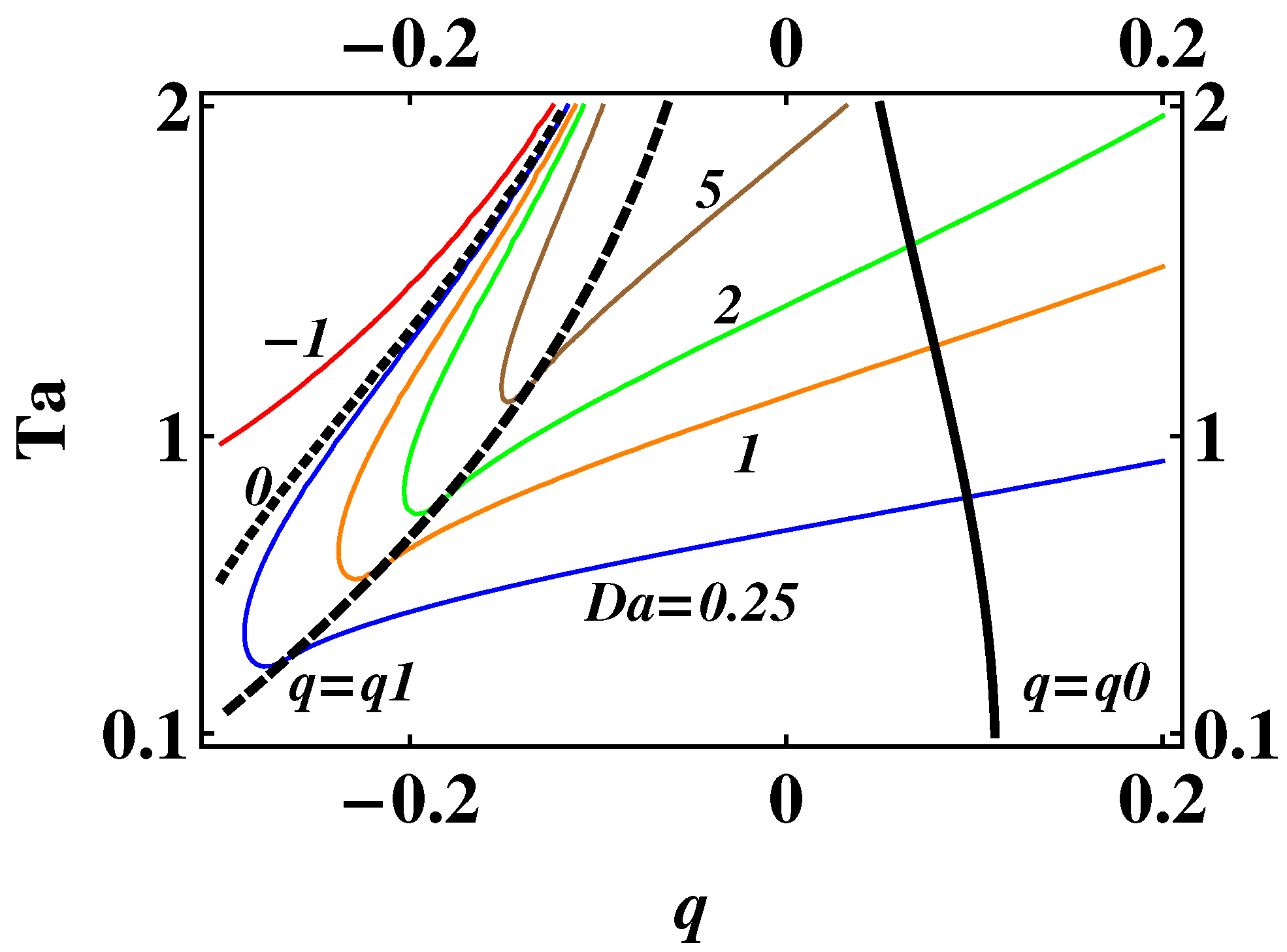
Within the region $q_1<q<q_0$, M and k are either both negative or both positive, which, according to equation (161), provides the positiveness of the interval $T_4-T_3$ of Bob’s proper time for segment (4) of his trip. It is not the case for the regions $q<q_1$ and $q>q_0$ which implies that, for the parameter values outside the region $q_1<q<q_0$, the solution is physically meaningless, or, what is the same, the scenario of Bob’s motion cannot be implemented. Contours of equal values of $Da$ in the plane $(q,T_a)$ are shown in Figure 2. The lines $q_1\left(T_a\right)$ (dashed) and $q_0\left(T_a\right)$ (solid), defined by Equations (162) and (160), bound the region $q_1<q<q_0$ where the results are meaningful. It is seen that, for the considered particular case of a general scenario, there is no possibility for a negative differential aging. The contours $Da<0$, which also appear in the graph, lie in the ’nonphysical’ region $q<q_1$.

Note that, in the special case considered in this subsection, there are only two parameters $G_1$ and $T_1$ available for Bob to control the scenario of his motion—all the rest, in particular, the acceleration $G_4$ and time of motion $T_4-T_3$ at the fourth segment of Bob’s motion, are determined by the value of $q=g/G_1$. Therefore, the possibilities for Bob to arrange his trip so that he could reach a desired object and return within a desired time period are restricted. Possibilities for choosing parameters of Bob’s trip are further narrowed down by the condition $q_1<q<q_0$ which can result in the accelerations required for arranging Bob’s trip in a desired way becoming infeasible. In the next subsection, the results of the analysis for a general scenario of Bob’s motion, when it is possible for Bob to choose not only the desired object and time of return but also the sign of a differential aging, are presented.

7.4. Accelerated Home Twin: General Case

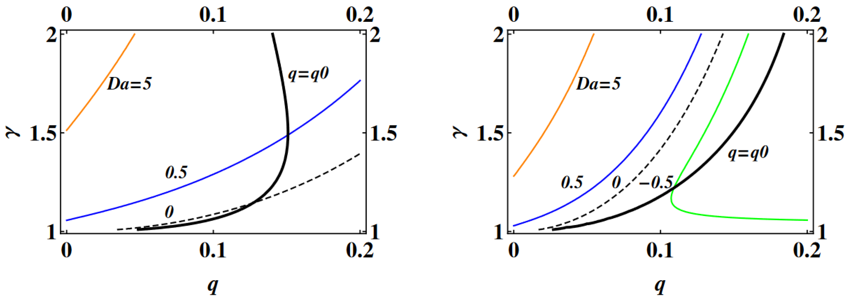
For a general scenario of Bob’s motion, the analysis reveals (we omit the details of calculations) that, depending on a combination of the parameters g, $G_1$, $G_2$, $G_3$, $T_1$, $T_2$, $T_3$, $T_u$, and $T_b$, the differential aging may be both positive and negative, and that negative differential aging can be achieved for reasonable values of the parameters. For $q<0$, the differential aging is always positive but for $q>0$ different possibilities may arise. To illustrate this, in Figure 3, contours of equal values of $Da$ in the plane $(q,\gamma )$ are shown for two sets of the remaining parameters. It should be remembered while considering the graphs that the results are meaningful only in the region $q<q_0$ (left of the solid line $q=q_0$). Another condition of validity of the results, $q>q_1$, does not play a role since, for the parameter values chosen for Figure 3, the curve $q=q_1$ lies in the region of $q<0$. It is seen that, for the set of parameters corresponding to Figure 3 (left), there is no possibility for a negative differential aging; the contours $Da<0$, which should be right of the dashed line $Da=0$, lie in the nonphysical region $q>q_0$. Such a possibility exists for the values of ${\gamma }_2$, $k_2$, $k_3$, $T_u$ and $T_b$ corresponding to Figure 3 (right). To show that negative values of the differential aging are achieved for reasonable values of Bob’s acceleration at the segment (4), variation of $Da$ and k along the lines intersecting the contour $Da=0$ in Figure 3 (right) is shown in Figure 4.

In general, Bob can arrange his trip to a desired object with a desired time of return such that the differential aging is of a desired sign, or, in other words, he can choose whether he wishes to find Alice younger or older than himself. If, for example, Bob chooses the parameters of his trip based on the distance to the point of destination and the time passed for Alice before his return, it imposes some relations on the parameters, but still freedoms remain. Let us consider two different feasible scenarios of Bob’s trip, with the same distance d to destination and time of return $t_R$ but with different signs of the differential aging $Da$. The first scenario corresponds to the point ($q=0.1,\gamma =1.8$) in Figure 3 (left). For that set of parameters, the calculated last segment acceleration and differential aging are $k=1.6$ and $Da=2.1$, and the corresponding distance to destination and time of return are $d\approx 9$ and $t_R\approx 12$. The second scenario corresponds to the point ($q=0.1,\gamma =1.3$) in Figure 3 (right), for which calculations give $k=1.6$ (incidentally the same as in the first scenario) and $Da=-0.26$ with approximately the same distance to destination and time of return as in the first scenario: $d\approx 9$ and $t_R\approx 12$. To get an idea of the above values in ordinary units, one has to choose the value of the first segment acceleration, $G_1$, which serves as a scale for non-dimensional variables. (One should remember that, in the system of units used, the values of g, t, and V are related to the values in ordinary units by $g=g^{*}/{\left(c^{*}\right)}^2$, $t=c^{*}{t}^{*}$, and $V=V^{*}/c^{*}$.).

8. Discussion

The analysis of the present paper reveals that, besides the relativistic symmetry expressed by the Lorentz group of coordinate transformations which leave invariant the Minkowski metric (2) of space-time of inertial frames, there is one more relativistic symmetry expressed by a group of coordinate transformations leaving invariant the space-time metric (3) of the frames with a constant proper-acceleration. It is remarkable that, in flat space-time, only those two relativistic symmetries, corresponding to groups of continuous transformations that leave invariant the metric (1) of space-time of extended rigid reference frames, exist. Therefore, the new relativistic symmetry identified in the present study should be considered on an equal footing with the Lorentz symmetry. (As it is clarified in the Introduction, the fact, that the metric (3) admits a diffeomorphism (6) into the Minkowski metric (1), in no way means equivalence of the groups of invariance of those two metrics or, what is the same, equivalence of the two relativistic symmetries.) In the context of the relativity principle, the existence of a space-time symmetry means that physical laws should maintain their form under the symmetry group transformations, or, in other terms, be the same regardless of the frame of reference used for description of the processes governed by the laws. The form of physical laws invariant under that new symmetry can be deduced in the same way as it is done in the case of Lorentz symmetry. It is, in particular, straightforward to proceed to deducing the form of the laws of free particle dynamics and electrodynamics in accelerated frames using the principle of least action with the form of the interval corresponding to the new relativistic symmetry.

It is worth clarifying that by the ’laws of physics in accelerated frames’ we mean the laws applied by an observer in the accelerated frame for description of the processes she/he observes. The motivation for developing the framework for such a description is twofold. On one side, it is evidently more convenient for the observer fixed in the accelerated frame to express the metric and the laws using the coordinates and variables defined by the observer, which allows the non-inertial observer to perform experiments and interpret the results of the experiments without making reference to inertial frames. On the other side, it is not completely clear how the physical laws stated in inertial frames can be applied to the description of processes from the point of view of observers in accelerated frames. Using the coordinate transformations from inertial to accelerated frames (inverse to (6)) can provide a description of only kinematic phenomena. A description of dynamic and electrodynamic phenomena in accelerated frames on the basis of the laws valid in inertial frames requires transformations of the variables figuring in the laws (like momentum, energy, electric and magnetic field intensities, and the electromagnetic field tensor) from inertial to accelerated frames. Defining the transformations on the basis of the coordinate transformations using the tensor calculus constructions is, in general, inconsistent. The coordinate transformations (6) (or (7)) do not represent a group of transformations within a set of equivalent frames related by the relativity principle, like the Lorentz transformation does, and so cannot serve as a basis for tensor calculus. For the same reason, formulating the physical laws in accelerated frames by replacing the usual derivatives in the inertial frame laws by covariant derivatives based on the transformations (6) is also unjustified. Further, using the equivalence principle for descriptions of, for example, electromagnetic phenomena, besides the fact that it is valid only locally, involves some subtle points and assumptions, and, even in the simple case of a single charged particle, the results obtained by different authors do not always agree with each other (see, e.g., the discussion in [9]). Using a comoving inertial frame for the description of dynamic and electrodynamic processes in an accelerated frame inevitably involves assumptions (which, in general, cannot be justified), for example, regarding the influence of the acceleration on the electric and magnetic field intensities and behavior of devices measuring them. (Even when the comoving inertial frame is used for a purely kinematic description of the processes in an accelerated frame, it involves some (unjustified) assumptions such as, for example, the ‘clock hypothesis’ which states that the rate of an accelerated clock is equal to that of a comoving unaccelerated clock.).

At the same time, deducing the form of physical laws in accelerated frames on the basis of the relativistic symmetry and corresponding group transformations in a way, similar to that used for developing the laws of physics on the basis of Lorentz symmetry and Lorentz transformations in special relativity, is straightforward and consistent from the point of view of the relativity principle. A possibility, that the laws developed in such a way could predict some new phenomena that should be observed by an observer in an accelerated frame, may serve as one more motivation for doing that work. Of course, those laws and phenomena should be subject to confirmation by experiments, similar to the laws of special relativity in the period of its development. (Nowadays, the situation is inverse in a sense. The Lorentz symmetry is considered to be a fundamental constraint for physical theories).

One more point deserves discussion. In the context of the present study, the concept of relativity, roughly speaking, is the idea that physics should appear to be the same in all uniformly accelerating frames, or, in a more rigorous formulation, that the equations expressing physical laws should have the same form in all the frames of that class. However, one may recall the Galilean formulation of the principle of relativity as the idea that uniform motion is undetectable by mechanical experiments. If we extend the Galilean principle of relativity to accelerated frames and to any physical experiments, it would imply that accelerated motion should be undetectable by experiments performed by an observer in an accelerated frame. This evidently contradicts the fact that the observer’s acceleration can be detected by her/him using some kind of accelerometer.

Nevertheless, in the framework of the present analysis, the fact that acceleration is detectable is not in contradiction with the relativity principle as the idea of relativistic invariance of physical laws. The point is that the value of acceleration g is a variable that takes part in the group transformations. The value of g transforms from frame to frame together with other variables in such a way that the functional form of the interval between two events and the functional form of equations governing processes in an accelerated frame remain the same. Correspondingly, the value of acceleration should take part in the invariant forms of physical laws on equal footing with other variables. The laws should even include the possibility of determining the value of that parameter by experiments but it in no way spoils the relativistic symmetry.

In that connection, it is worthwhile to recall that the relativity principle of the standard special relativity is violated on cosmological scales by the possibility of detecting the absolute motion speed relative to the CMB frame. In the analysis of [39], this conceptual difficulty is remedied by treating a parameter related to the absolute velocity as a variable that takes part in the group transformations. Relativistic invariance is preserved that way and the theory can be developed from the same general principles as in standard special relativity. Applying the ’relativity with a preferred frame’, extended to particle dynamics, electrodynamics, and general relativity, to the interpretation of the observational data on cosmological scales [39,40,41] allows to resolve some challenges without introducing new physics, for example, to fit the SNIa data into the theory without introducing ‘dark energy’.

To conclude, identifying the new relativistic symmetry and the corresponding group transformations in the present study paves the way for defining the forms of physical laws that satisfy the relativity principle for accelerated frames. This should be a subject for future study.

References

- Einstein, A. Uber das Relativitatsprinzip und die aus demselben gezogene Folgerungen, Jahrbuch der Radioaktivitaet und Elektronik [On the Relativity Principle and the Conclusions Drawn from It]. In The Collected Papers of Albert Einstein, The Swiss Years: Writings, 1900–1909, Volume 2; Stachel, J., Cassidy, D.C., Renn, J., Schulmann, R., Eds.; Princeton University Press: Princeton, NJ, USA; pp. 252–311.
- Fock, V. The Theory of Space, Time, and Gravitation, 2nd ed.; Pergamon Press: Oxford, UK, 1964. [Google Scholar]
- Synge, J.L. Relativity: The General Theory; North-Holland: Amsterdam, The Netherlands, 1966. [Google Scholar]
- Landau, L.D.; Lifshitz, E.M. The Classical Theory of Fields; Pergamon Press: Oxford, UK, 1971. [Google Scholar]
- Møller, C. On Homogeneous Gravitational Fields in the General Theory of Relativity and the Clock Paradox. Kgl. Danske Vid. Sel. 1943, 20, 1–24. [Google Scholar]
- Lass, H. Accelerated Frames of Reference and the Clock Paradox. Am. J. Phys. 1963, 31, 274–276. [Google Scholar] [CrossRef]
- Marsh, L.M. Relativistic Accelerated Systems. Am. J. Phys. 1965, 33, 934–938. [Google Scholar] [CrossRef]
- Romain, J.E. Remarks on a Coordinate Transformation to an Accelerated Frame of Reference. Am. J. Phys. 1964, 32, 279–285. [Google Scholar] [CrossRef]
- Rohrlich, F. The Principle of Equivalence. Ann. Phys. 1963, 22, 169–191. [Google Scholar] [CrossRef]
- Landsberg, P.T.; Bishop, N.T. Gravitational Redshift and the Equivalence Principle. Found. Phys. 1976, 6, 727–737. [Google Scholar] [CrossRef]
- Desloge, E.A.; Philpott, R.J. Uniformly Accelerated Reference Frames in Special Relativity. Am. J. Phys. 1987, 55, 252–261. [Google Scholar] [CrossRef]
- Minguzzi, E. The Minkowski metric in non-inertial observer radar coordinates. Am. J. Phys. 2005, 73, 1117–1121. [Google Scholar] [CrossRef] [Green Version]
- Koks, D. The Uniformly Accelerated Frame as a Test Bed for Analysing the Gravitational Redshift. Universe 2021, 7, 4. [Google Scholar] [CrossRef]
- Munoz, G.; Jones, P. The Equivalence Principle, Uniformly Accelerated Reference Frames, and the Uniform Gravitational Field. Am. J. Phys. 2010, 78, 377–383. [Google Scholar] [CrossRef] [Green Version]
- Tilbrook, D. General Coordinatisations of the Flat Space–Time of Constant Proper-acceleration. Aust. J. Phys. 1997, 50, 851–868. [Google Scholar] [CrossRef] [Green Version]
- Rindler, W. Essential Relativity; Springer: New York, NY, USA, 1977. [Google Scholar]
- Burde, G.I. Special Relativity Kinematics with Anisotropic Propagation of Light and Correspondence Principle. Found. Phys. 2016, 46, 1573–1597. [Google Scholar] [CrossRef]
- Bluman, G.W.; Kumei, S. Symmetries and Differential Equations; Applied Mathematical Sciences; Springer: New York, NY, USA, 1989; Volume 81. [Google Scholar]
- Olver, P.J. 1993 Applications of Lie Groups to Differential Equations; Graduate Texts in Mathematics; Springer: New York, NY, USA, 1993; Volume 107. [Google Scholar]
- Ibragimov, N.H. (Ed.) CRC Handbook of Lie Group Analysis of Differential Equations; CRC Press: Boca Raton, FL, USA, 1996; Volume 2. [Google Scholar]
- Misner, C.W.; Thorne, K.S.; Wheeler, J.A. Gravitation; Freeman and Company: New York, NY, USA, 1973. [Google Scholar]
- Rindler, W. Kruskal Space and the Uniformly Accelerated Frame. Am. J. Phys. 1966, 34, 1174–1178. [Google Scholar] [CrossRef]
- Bourgin, D.G. The New Relativity. Phys. Rev. 1936, 50, 864–868. [Google Scholar] [CrossRef]
- Hill, E.L. On Accelerated Coordinate Systems in Classical and Relativistic Mechanics. Phys. Rev. 1945, 67, 358–363. [Google Scholar] [CrossRef]
- Hsu, J.-P.; Hsu, L. Four-dimensional symmetry of taiji relativity and coordinate transformations based on a weaker postulate for the speed of light—II. Nuovo Cim. 1997, 112B, 575–589. [Google Scholar]
- Hsu, J.-P.; Hsu, L. Generalized Lorentz Transformations for Linearly Accelerated Frames with Limiting Four-Dimensional Symmetry. Chin. J. Phys. 1997, 35, 407–417. [Google Scholar]
- Hsu, J.-P.; Fine, D. Remarks on the Development of the Gravitational and Yang-Mills Fields and Accelerated Frames. In 100 Years of Gravity and Accelerated Frames: The Deepest Insights of Einstein and Yang-Mills; Hsu, J.-P., Fine, D., Eds.; Advanced Series on Theoretical Physical Science; World Scientific Publishing: Singapore, 2005; Volume 9. [Google Scholar]
- Pauli, W. Theory of Relativity; Pergamon Press: Oxford, UK, 1958. [Google Scholar]
- Marder, L. Time and the Space-Traveller; George Allen & Unwin: London, UK, 1971. [Google Scholar]
- Taylor, F.; Wheeler, J.A. Spacetime Physics; Freeman: San Francisco, CA, USA, 1966. [Google Scholar]
- Shuler, R.L., Jr. The twins clock paradox history and perspectives. J. Mod. Phys. 2014, 5, 1062–1078. [Google Scholar] [CrossRef] [Green Version]
- Møller, C. The Theory of Relativity; Clarendon Press: Oxford, UK, 1962. [Google Scholar]
- Grøn, Ø. A Symmetrical Version of the Clock Paradox. Eur. J. Phys. 1988, 9, 71–74. [Google Scholar] [CrossRef]
- Eriksen, E.; Grøn, Ø. Relativistic Dynamics in Uniformly Accelerated Reference Frames with Application to the Clock Paradox. Eur. J. Phys. 1990, 11, 39–44. [Google Scholar] [CrossRef]
- Coleman, C.F. When is Simultaneity Transitive in Special Relativity? Eur. J. Phys. 1989, 10, 235–238. [Google Scholar] [CrossRef]
- Boughn, S.P. The Case of the Identically Accelerated Twins. Am. J. Phys. 1989, 57, 791–793. [Google Scholar] [CrossRef]
- Wu, T.Y.; Lee, Y.C. The Clock Paradox in the Relativity Theory. Intern. J. Theoretical Phys. 1972, 5, 307–323. [Google Scholar] [CrossRef]
- Minguzzi, E. Differential Aging from Acceleration: An Explicit Formula. Am. J. Phys. 2005, 73, 876–880. [Google Scholar] [CrossRef] [Green Version]
- Burde, G.I. Cosmological Models Based on Relativity with a Privileged Frame. Int. J. Mod. Phys. D 2020, 29, 2050038. [Google Scholar] [CrossRef]
- Burde, G.I. Particle Dynamics and GZK Limit in Relativity with a Preferred Frame. Astropart. Phys. 2021, 126, 102526. [Google Scholar] [CrossRef]
- Burde, G.I. Lorentz Violation by the Preferred Frame Effects and Cosmic and Gamma Ray Propagation. Galaxies 2021, 9, 119. [Google Scholar] [CrossRef]
- Page, L. A New Relativity. Paper I. Fundamental Principles and Transformations Between Accelerated Systems. Phys. Rev. 1936, 49, 254–268. [Google Scholar] [CrossRef]
- Engstrom, H.T.; Zorn, M. The Transformation of Reference Systems in the Page Relativity. Phys. Rev. 1936, 49, 701–702. [Google Scholar] [CrossRef]
- Robertson, H.P. An Interpretation of Page’s “New Relativity”. Phys. Rev. 1936, 49, 755–760. [Google Scholar] [CrossRef]
Figure 1.
Graphs of Bob’s (dashed) and Alice’s (solid) motions in the inertial frame for (left) and (right).
Figure 2.
Isolines of on the plane (different colors correspond to different values of ) and boundaries of the region of validity of the solution.
Figure 3.
Isolines of (different colors correspond to different values of ) on the plane for two different sets of parameters (left and right panels).
Figure 4.
Variation of (blue) and k (yellow) along the vertical (left) and horizontal (right) lines in Figure 3 (right).
Disclaimer/Publisher’s Note: The statements, opinions and data contained in all publications are solely those of the individual author(s) and contributor(s) and not of MDPI and/or the editor(s). MDPI and/or the editor(s) disclaim responsibility for any injury to people or property resulting from any ideas, methods, instructions or products referred to in the content. |
© 2023 by the author. Licensee MDPI, Basel, Switzerland. This article is an open access article distributed under the terms and conditions of the Creative Commons Attribution (CC BY) license (https://creativecommons.org/licenses/by/4.0/).
Share and Cite
MDPI and ACS Style
Burde, G.I. Groups of Coordinate Transformations between Accelerated Frames. Symmetry 2023, 15, 1226. https://doi.org/10.3390/sym15061226
AMA Style
Burde GI. Groups of Coordinate Transformations between Accelerated Frames. Symmetry. 2023; 15(6):1226. https://doi.org/10.3390/sym15061226
Chicago/Turabian StyleBurde, Georgy I. 2023. "Groups of Coordinate Transformations between Accelerated Frames" Symmetry 15, no. 6: 1226. https://doi.org/10.3390/sym15061226
Note that from the first issue of 2016, this journal uses article numbers instead of page numbers. See further details here.