The Solitary Solutions for the Stochastic Jimbo–Miwa Equation Perturbed by White Noise

Abstract

We study the (3+1)-dimensional stochastic Jimbo–Miwa (SJM) equation induced by multiplicative white noise in the Itô sense. We employ the Riccati equation mapping and He’s semi-inverse techniques to provide trigonometric, hyperbolic, and rational function solutions of SJME. Due to the applications of the Jimbo–Miwa equation in ocean studies and other disciplines, the acquired solutions may explain numerous fascinating physical phenomena. Using a variety of 2D and 3D diagrams, we illustrate how white noise influences the analytical solutions of SJM equation. We deduce that the noise destroys the symmetry of the solutions of SJM equation and stabilizes them at zero.

1. Introduction

Nonlinear evolution equations (NEEs) are used to simulate a wide range of complicated real-world phenomena. NEEs are engaged in various fields of science and engineering, including plasma physics, astrophysics, cosmology, acoustics, electrochemistry, chemical reaction, optical fiber, biology, ecology, mechanics, fluid dynamics and electromagnetic theory. As a result, it is necessary to find the solutions to these NEEs. In recent years, many techniques for solving NEEs, including the tanh–coth method [1], generalized auxiliary equation [2], extended direct algebraic method [3], extended $(G^{\prime }/G^2)$-expansion technique [4], Riccati equation method [5], He’s semi-inverse method [6], sine-cosine method [7], auxiliary equation method [8], Jacobi elliptic function method [9], F-expansion technique [10], Lie symmetry method [11], $(G^{\prime }/G)$-expansion [12], $exp(-\varphi (\varsigma \left)\right)$-expansion [13], etc., have been presented.

More generally, stochastic NEEs are utilized to address systems in physics, biology and chemistry that are subject to random influences. During the past few decades, the significance of including randomness into complex system models has been recognized. The use of stochastic NEEs for developing mathematical models of complex processes is on the rise in many fields, including materials sciences, condensed matter climate, finance, information systems, electrical engineering, biophysics and physics system modeling [14,15]. In recent years, analytical solutions for some stochastic NEEs have been acquired, for example [16,17,18,19,20] and the references therein.

Stochastic effects in NEEs must thus be considered. The (3+1)-dimensional stochastic Jimbo–Miwa (SJM) equation driven by a multiplicative noise is considered here:

$$2{\mathcal{V}}_{yt}+{\mathcal{V}}_{xxxy}+3{\mathcal{V}}_x{\mathcal{V}}_{xy}+3{\mathcal{V}}_{xx}{\mathcal{V}}_y-3{\mathcal{V}}_{xz}=2\lambda {\mathcal{V}}_y{\mathcal{G}}_t,$$

(1)

where $\mathcal{V}=\mathcal{V}(x,y,z,t)$ is an analytic function,$\mathcal{G}=\mathcal{G}\left(t\right)$ is the standard Wiener process (white noise),$\lambda$ represents the noise intensity. Equation (1), with $\lambda =0$, was found by Jimbo and Miwa [21]. Equation (1) is the second one in the KP-hierarchy. Although Equation (1) is nonintegrable, a variety of methods have been proposed to acquire the solutions, including the extended rational expansion method [22], homogeneous balance method [23], extended homogeneous balance method [24], generalized F-expansion method [25], multi-linear variable separation approach [26], Hirota’s bilinear method [27], tanh–coth method [28] and Riccati equation mapping method [29]. The exact stochastic solutions to Equation (1) was not obtained until now.

The objective of this work is to determine exact stochastic solutions of SJM Equation (1). He’s semi-inverse method (HSI-method) and Riccati equation mapping method (REM-method) are utilized to obtain these solutions. Some previous results, including those presented in [29], have been extended. The stochastic term in Equation (1) provides solutions that are incredibly helpful for characterizing a variety of significant physical phenomena. In addition, we provide a large number of graphs in MATLAB to investigate the effect of white noise on the solution of the SJM Equation (1).

This is a brief summary of the article: Section 2 derives the wave equation of SJM Equation (1). Section 3 focuses on obtaining exact solutions for the SJM equation. Section 4 investigates how white noise affects the solutions of the SJM equation. Finally, the findings of the article are presented.

2. Wave Equation for SJM Equation

To derive the wave equation of SJM Equation (1), we use

$$\mathcal{V}(x,y,z,t)=\mathcal{Y}\left(\xi \right)e^{(\lambda \mathcal{G}\left(t\right)-\frac{1}{2}{\lambda }^{2}t)},\xi ={\xi }_{1}x+{\xi }_{2}y+{\xi }_{3}z+{\xi }_{4}t,$$

(2)

where the function $\mathcal{Y}$ is a deterministic, ${\xi }_1,{\xi }_2,$ ${\xi }_3$ and ${\xi }_4$ are undefined constants. We observe that

$$\begin{array}{ccc}\hfill {\mathcal{V}}_x& =& {\xi }_1{\mathcal{Y}}^{\prime }{e}^{(\lambda \mathcal{G}\left(t\right)-\frac{1}{2}{\lambda }^{2}t)},{\mathcal{V}}_y={\xi }_2{\mathcal{Y}}^{\prime }{e}^{(\lambda \mathcal{G}\left(t\right)-\frac{1}{2}{\lambda }^{2}t)},\hfill \\ \hfill {\mathcal{V}}_{xz}& =& {\xi }_1{\xi }_3{\mathcal{Y}}^{″}{e}^{(\lambda \mathcal{G}\left(t\right)-\frac{1}{2}{\lambda }^{2}t)},{\mathcal{V}}_{xx}={\xi }_1^2{\mathcal{Y}}^{″}{e}^{(\lambda \mathcal{G}\left(t\right)-\frac{1}{2}{\lambda }^{2}t)},\hfill \\ \hfill {\mathcal{V}}_{xy}& =& {\xi }_1{\xi }_2{\mathcal{Y}}^{″}{e}^{(\lambda \mathcal{G}\left(t\right)-\frac{1}{2}{\lambda }^{2}t)},{\mathcal{V}}_{xxxy}={\xi }_2{\xi }_1^3{\mathcal{Y}}^{″″}{e}^{(\lambda \mathcal{G}\left(t\right)-\frac{1}{2}{\lambda }^{2}t)},\hfill \\ \hfill {\mathcal{V}}_{yt}& =& [{\xi }_2{\xi }_4{\mathcal{Y}}^{″}+\lambda {\xi }_2{\mathcal{Y}}^{\prime }{\mathcal{G}}_t]e^{(\lambda \mathcal{G}\left(t\right)-\frac{1}{2}{\lambda }^{2}t)}.\hfill \end{array}$$

(3)

Substituting Equation (3) into Equation (1), yields

$$(2{\xi }_2{\xi }_4-3{\xi }_1{\xi }_3){\mathcal{Y}}^{″}+{\xi }_2{\xi }_1^3{\mathcal{Y}}^{″″}+6{\xi }_2{\xi }_1^2{\mathcal{Y}}^{\prime }{\mathcal{Y}}^{″}{e}^{(\lambda \mathcal{G}\left(t\right)-\frac{1}{2}{\lambda }^{2}t)}=0.$$

(4)

When we take into account the expectations on both sides, we get

$$(2{\xi }_2{\xi }_4-3{\xi }_1{\xi }_3){\mathcal{Y}}^{″}+{\xi }_2{\xi }_1^3{\mathcal{Y}}^{″″}+6{\xi }_2{\xi }_1^2{\mathcal{Y}}^{\prime }{\mathcal{Y}}^{″}{e}^{-\frac{1}{2}{\lambda }^{2}t}\mathbb{E}{e}^{\left(\lambda \mathcal{G}\right(t\left)\right)}=0.$$

(5)

Since $\mathcal{G}\left(t\right)$ is white noise, then $\mathbb{E}{e}^{\lambda \mathcal{G}\left(t\right)}=e^{\left(\frac{1}{2}{\lambda }^{2}t\right)}$, Equation (5) turns into

$${\mathcal{Y}}^{″″}+{\ell }_1{\mathcal{Y}}^{″}+2{\ell }_2{\mathcal{Y}}^{\prime }{\mathcal{Y}}^{″}=0,$$

(6)

where

$${\ell }_1=\frac{(2{\xi }_2{\xi }_4-3{\xi }_1{\xi }_3)}{{\xi }_2{\xi }_1^3}\mathrm{and}{\ell }_2=\frac{3}{{\xi }_1}.$$

(7)

Integrating Equation (6), yields

$${\mathcal{Y}}^{‴}+{\ell }_1{\mathcal{Y}}^{\prime }+{\ell }_2{\left({\mathcal{Y}}^{\prime }\right)}^2=C,$$

where C is the integral constant. We assume $C=0$ to get

$${\mathcal{Y}}^{‴}+{\ell }_1{\mathcal{Y}}^{\prime }+{\ell }_2{\left({\mathcal{Y}}^{\prime }\right)}^2=0.$$

(8)

3. Exact Solutions of SJM Equation

Two different methods, such as the REM method and HSI method, are used to obtain the solutions to Equation (8). As a result, the solutions to the SJM Equation (1) are found.

3.1. Application of the REM-Method

The Riccati–Bernoulli equation has the form:

$${\mathcal{Y}}^{\prime }=s{\mathcal{Y}}^2+r\mathcal{Y}+p,$$

(9)

where $s,r,p$ are constants. Using Equation (9), we have

$${\mathcal{Y}}^{‴}=6s^3{\mathcal{Y}}^4+12r{s}^2{\mathcal{Y}}^3+(8p{s}^2+7s{r}^2){\mathcal{Y}}^2+(r^3+8rsp)\mathcal{Y}+(r^2+2s{p}^2).$$

(10)

Substituting Equations (9) and (10) into (8), we get

$$\begin{array}{c}(6s^3+s^2{\ell }_2){\mathcal{Y}}^4+(12r{s}^2+2rs{\ell }_2){\mathcal{Y}}^3+(8p{s}^2+7s{r}^2+s{\ell }_1+2ps{\ell }_2+r^2{\ell }_2){\mathcal{Y}}^2\\ +(r^3+8rsp+r{\ell }_1+2pr{\ell }_2)\mathcal{Y}+(r^2+2s{p}^2+p{\ell }_1+p^2{\ell }_2)=0.\end{array}$$

Equating each coefficient of ${\mathcal{Y}}^k$ to zero yields

$$6s^3+s^2{\ell }_2=0,$$

$$12r{s}^2+2rs{\ell }_2=0,$$

$$8p{s}^2+7s{r}^2+s{\ell }_1+2ps{\ell }_2+r^2{\ell }_2=0,$$

$$r^3+8rsp+r{\ell }_1+2pr{\ell }_2,$$

and

$$r^2+2s{p}^2+p{\ell }_1+p^2{\ell }_2=0.$$

By solving these equations, we find

$$s=\frac{-{\ell }_2}{6},r=0,\mathrm{and}p=\frac{-3{\ell }_1}{2{\ell }_2}.$$

(11)

Now, we can rewrite Equation (9) as

$$\frac{d\mathcal{Y}}{{\mathcal{Y}}^2+\left(\frac{p}{s}\right)}=sd\xi .$$

(12)

There are different sets relying on p and s, as follows:

Family I: When $ps>0,$ thus, the solutions of Equation (9) are:

$${\mathcal{Y}}_1\left(\xi \right)=\sqrt{\frac{p}{s}}tan\left(\sqrt{ps}\xi \right),$$

$${\mathcal{Y}}_2\left(\xi \right)=-\sqrt{\frac{p}{s}}cot\left(\sqrt{ps}\xi \right),$$

$${\mathcal{Y}}_3\left(\xi \right)=\sqrt{\frac{p}{s}}\left(tan\left(\sqrt{4ps}\xi \right)\pm sec\left(\sqrt{4ps}\xi \right)\right),$$

$${\mathcal{Y}}_4\left(\xi \right)=-\sqrt{\frac{p}{s}}\left(cot\left(\sqrt{4ps}\xi \right)\pm csc\left(\sqrt{4ps}\xi \right)\right),$$

$${\mathcal{Y}}_5\left(\xi \right)=\frac{1}{2}\sqrt{\frac{p}{s}}\left(tan\left(\frac{1}{2}\sqrt{ps}\xi \right)-cot\left(\frac{1}{2}\sqrt{ps}\xi \right)\right).$$

Then, the SJM Equation (1) has the solutions:

$${\mathcal{V}}_1(x,y,z,t)=\sqrt{\frac{p}{s}}tan\left(\sqrt{ps}\xi \right)e^{(\lambda \mathcal{G}\left(t\right)-\frac{1}{2}{\lambda }^{2}t)},$$

(13)

$${\mathcal{V}}_2(x,y,z,t)=-\sqrt{\frac{p}{s}}cot\left(\sqrt{ps}\xi \right)e^{(\lambda \mathcal{G}\left(t\right)-\frac{1}{2}{\lambda }^{2}t)},$$

(14)

$${\mathcal{V}}_3(x,y,z,t)=\sqrt{\frac{p}{s}}\left(tan\left(\sqrt{4ps}\xi \right)\pm sec\left(\sqrt{4ps}\xi \right)\right),e^{(\lambda \mathcal{G}\left(t\right)-\frac{1}{2}{\lambda }^{2}t)},$$

(15)

$${\mathcal{V}}_4(x,y,z,t)=-\sqrt{\frac{p}{s}}\left(cot\left(\sqrt{4ps}\xi \right)\pm csc\left(\sqrt{4ps}\xi \right)\right)e^{(\lambda \mathcal{G}\left(t\right)-\frac{1}{2}{\lambda }^{2}t)},$$

(16)

$${\mathcal{V}}_5(x,y,z,t)=\frac{1}{2}\sqrt{\frac{p}{s}}\left(tan(\frac{1}{2}\sqrt{ps}\xi )-cot(\frac{1}{2}\sqrt{ps}\xi )\right)e^{(\lambda \mathcal{G}\left(t\right)-\frac{1}{2}{\lambda }^{2}t)},$$

(17)

where $\xi ={\xi }_{1}x+{\xi }_{2}y+{\xi }_{3}z+{\xi }_{4}t.$

Family II: When $ps<0,$ thus the solutions of Equation (9) are:

$${\mathcal{Y}}_6\left(\xi \right)=-\sqrt{\frac{-p}{s}}tanh\left(\sqrt{-ps}\xi \right),$$

$${\mathcal{Y}}_7\left(\xi \right)=-\sqrt{\frac{-p}{s}}coth\left(\sqrt{-ps}\xi \right),$$

$${\mathcal{Y}}_8\left(\xi \right)=-\sqrt{\frac{-p}{s}}\left(tanh\left(\sqrt{-4ps}\xi \right)\pm i\mathrm{sech}\left(\sqrt{-4ps}\xi \right)\right),$$

$${\mathcal{Y}}_9\left(\xi \right)=-\sqrt{\frac{-p}{s}}\left(coth\left(\sqrt{-4ps}\xi \right)\pm \mathrm{csch}\left(\sqrt{-4ps}\xi \right)\right),$$

$${\mathcal{Y}}_{10}\left(\xi \right)=\frac{-1}{2}\sqrt{\frac{-p}{s}}\left(tanh\left(\frac{1}{2}\sqrt{-ps}\xi \right)+coth\left(\frac{1}{2}\sqrt{-ps}\xi \right)\right).$$

Then, the SJM Equation (1) has the solutions:

$${\mathcal{V}}_6(x,y,z,t)=-\sqrt{\frac{-p}{s}}tanh\left(\sqrt{-ps}\xi \right)e^{(\lambda \mathcal{G}\left(t\right)-\frac{1}{2}{\lambda }^{2}t)},$$

(18)

$${\mathcal{V}}_7(x,y,z,t)=-\sqrt{\frac{-p}{s}}coth\left(\sqrt{-ps}\xi \right)e^{(\lambda \mathcal{G}\left(t\right)-\frac{1}{2}{\lambda }^{2}t)},$$

(19)

$${\mathcal{V}}_8(x,y,z,t)=-\sqrt{\frac{-p}{s}}\left(tanh\left(\sqrt{-4ps}\xi \right)\pm i\mathrm{sech}\left(\sqrt{-4ps}\xi \right)\right)e^{(\lambda \mathcal{G}\left(t\right)-\frac{1}{2}{\lambda }^{2}t)},$$

(20)

$${\mathcal{V}}_9(x,y,z,t)=-\sqrt{\frac{-p}{s}}\left(coth\left(\sqrt{-4ps}\xi \right)\pm \mathrm{csch}\left(\sqrt{-4ps}\xi \right)\right)e^{(\lambda \mathcal{G}\left(t\right)-\frac{1}{2}{\lambda }^{2}t)},$$

(21)

$${\mathcal{V}}_{10}(x,y,z,t)=\frac{-1}{2}\sqrt{\frac{-p}{s}}\left(tanh(\frac{1}{2}\sqrt{-ps}\xi )+coth(\frac{1}{2}\sqrt{-ps}\xi )\right)e^{(\lambda \mathcal{G}\left(t\right)-\frac{1}{2}{\lambda }^{2}t)},$$

(22)

where $\xi ={\xi }_{1}x+{\xi }_{2}y+{\xi }_{3}z+{\xi }_{4}t.$

Family III: When $p=0,s\ne 0,$ then Equation (9) has the solution

$${\mathcal{Y}}_{11}\left(\xi \right)=\frac{-1}{s\xi }.$$

Hence, the SJM Equation (1) has the solution

$${\mathcal{V}}_{11}(x,y,z,t)=\left(\frac{-1}{s({\xi }_{1}x+{\xi }_{2}y+{\xi }_{3}z+{\xi }_{4}t)}\right)e^{(\lambda \mathcal{G}\left(t\right)-\frac{1}{2}{\lambda }^{2}t)}.$$

(23)

At the end of this subsection, we can deduce that the REM method is direct, effective and straightforward. Moreover, this method provide various kinds of solutions, for example trigonometric, hyperbolic and rational solutions, which explain numerous phenomena associated with the behavior of the Jimbo–Miwa equation.

Remark 1.

Putting $\lambda =0$ in Equations (13)–(23), identical solutions are given in [29].

3.2. Application of the HSI-Method

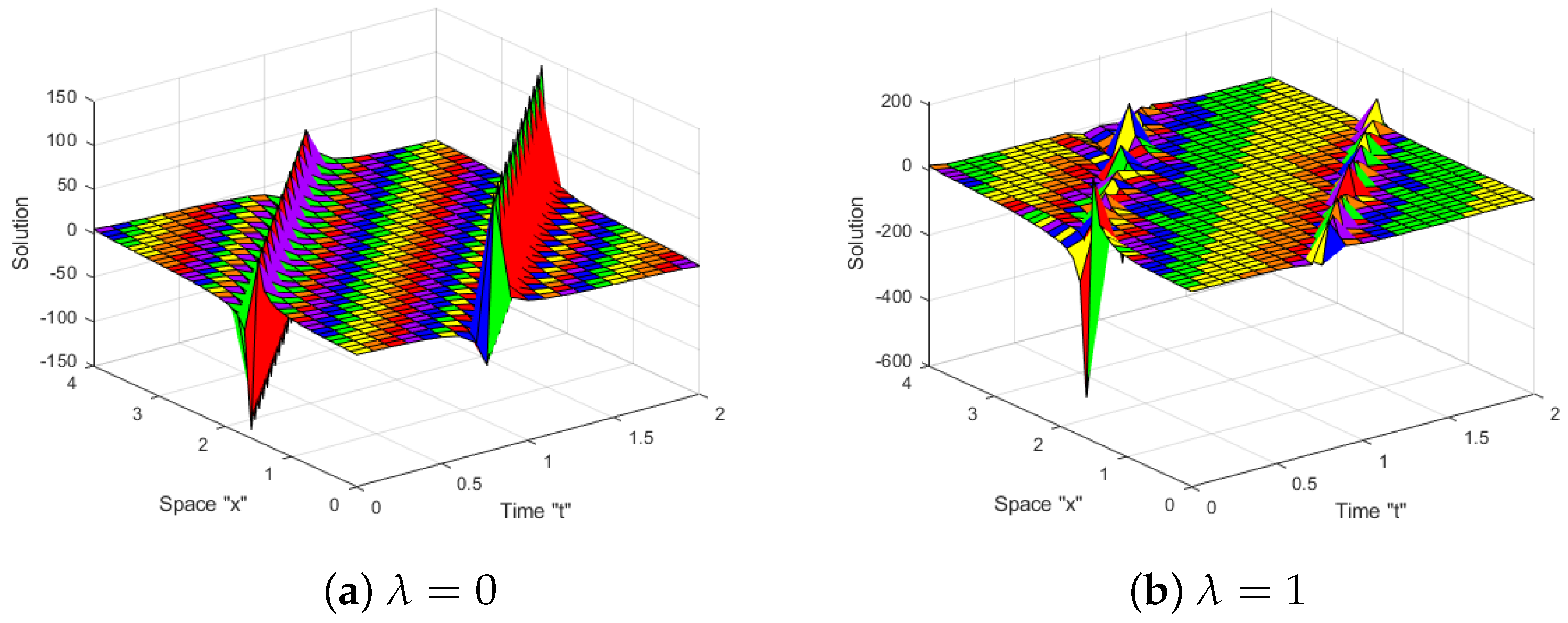
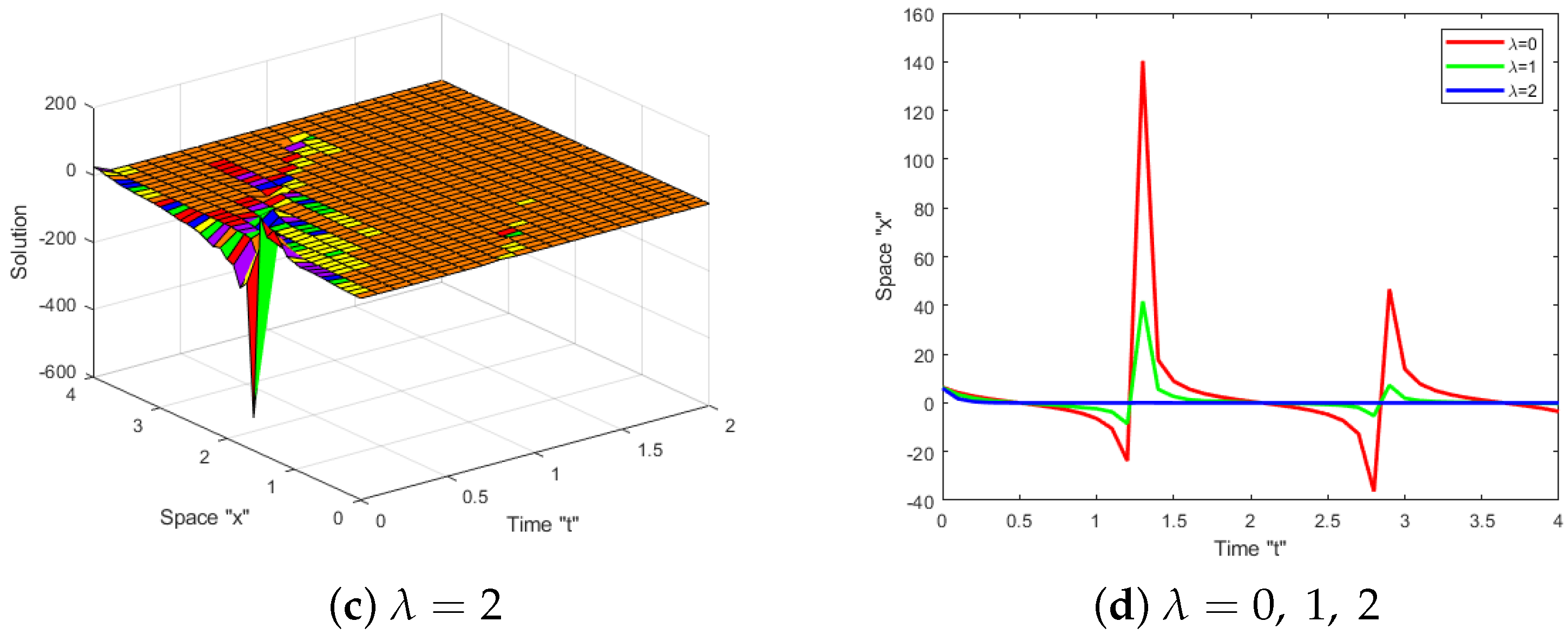
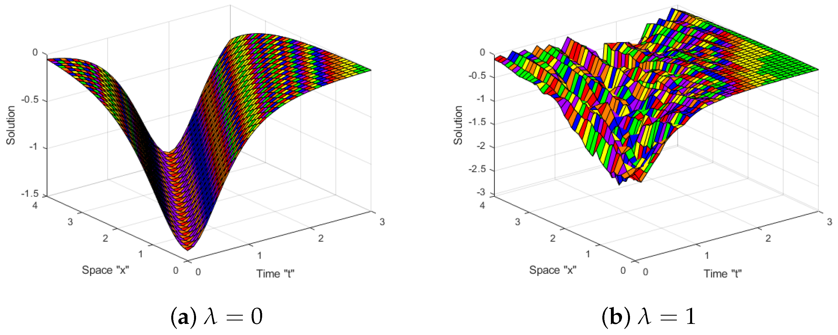
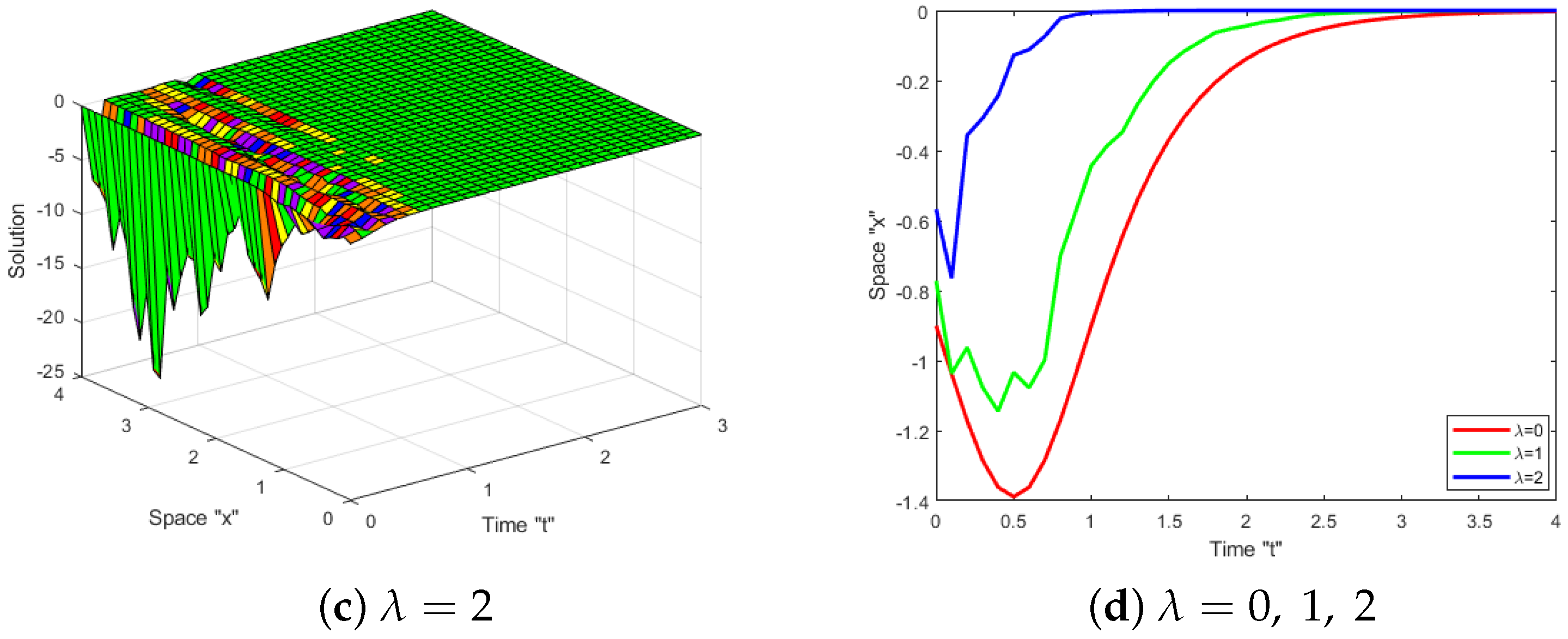
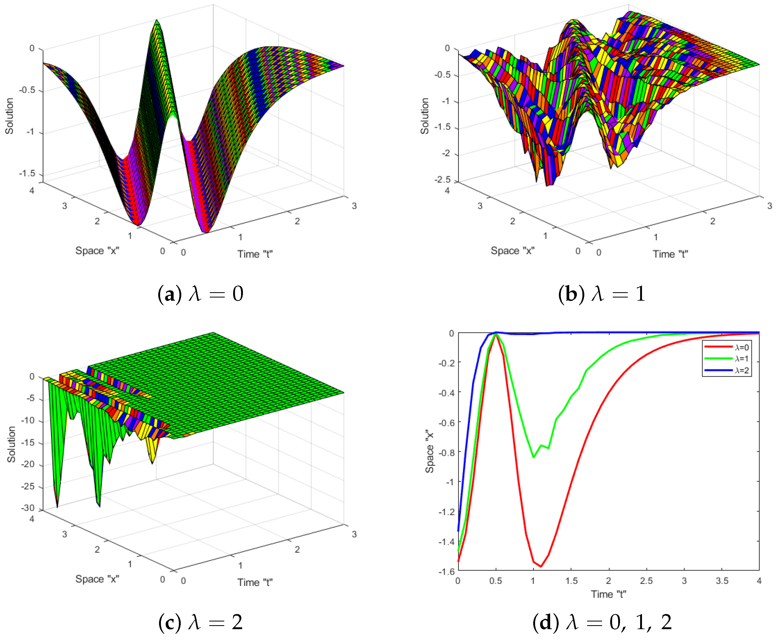
As stated in [30,31,32], we obtain the following variational formulations:

$$\mathbb{J}\left(\mathcal{Y}\right)={\int }_0^{\infty }\{\frac{1}{2}{\left({\mathcal{Y}}^{″}\right)}^2-\frac{1}{2}{\ell }_1{\left({\mathcal{Y}}^{\prime }\right)}^2+\frac{1}{3}{\ell }_2{\left({\mathcal{Y}}^{\prime }\right)}^3\}d\xi .$$

(24)

Now, let the solution of (6) take the form

$$\mathcal{Y}\left(\xi \right)=\mathcal{K}\mathrm{sech}\left(\xi \right),$$

(25)

where $\mathcal{K}$ is an unknown constant. Substituting Equation (25) into Equation (24), we have

$$\begin{array}{ccc}\hfill \mathbb{J}& =& \frac{1}{2}{\mathcal{K}}^2{\int }_0^{\infty }[{\mathrm{sech}}^2\left(\xi \right){tanh}^4\left(\xi \right)+{\mathrm{sech}}^4\left(\xi \right){tanh}^2\left(\xi \right)+{\mathrm{sech}}^6\left(\xi \right)\hfill \\ & & -{\ell }_1{\mathrm{sech}}^2\left(\xi \right){tanh}^2\left(\xi \right)+\frac{2}{3}{\ell }_2\mathcal{K}{\mathrm{sech}}^3\left(\xi \right){tanh}^3\left(\xi \right)]d\xi \hfill \\ & =& \frac{1}{2}{\mathcal{K}}^2{\int }_0^{\infty }[({\mathrm{sech}}^2\left(\xi \right)-{\ell }_1{\mathrm{sech}}^2\left(\xi \right){tanh}^2\left(\xi \right)+\frac{2}{3}{\ell }_2\mathcal{K}{\mathrm{sech}}^3\left(\xi \right){tanh}^3\left(\xi \right)]d\xi \hfill \\ & =& \frac{{\mathcal{K}}^2}{2}-{\ell }_1\frac{{\mathcal{K}}^2}{6}-\frac{2}{45}{\ell }_2{\mathcal{K}}^3.\hfill \end{array}$$

Making the following $\mathbb{J}$ stationary associated with $\mathcal{K}$

$$\frac{\partial \mathbb{J}}{\partial \mathcal{K}}=(1-\frac{1}{3}{\ell }_1)\mathcal{K}-\frac{2}{15}{\ell }_2{\mathcal{K}}^2=0.$$

(26)

Solving Equation (26) yields

$$\mathcal{K}=\frac{15-5{\ell }_1}{2{\ell }_2}.$$

Hence, Equation (6) has the solution

$$\mathcal{Y}\left(\xi \right)=\frac{15-5{\ell }_1}{6{\ell }_2}\mathrm{sech}\left(\xi \right).$$

Now, the solution of the SJM Equation (1) is

$$\mathcal{V}(x,y,z,t)=\frac{15-5{\ell }_1}{6{\ell }_2}\mathrm{sech}({\xi }_{1}x+{\xi }_{2}y+{\xi }_{3}z+{\xi }_{4}t)e^{(\lambda \mathcal{G}\left(t\right)-\frac{1}{2}{\lambda }^{2}t)}.$$

(27)

We may do the same with the solution (6), as follows

$$\mathcal{Y}\left(\xi \right)=\mathcal{N}\mathrm{sech}\left(\xi \right){tanh}^2\left(\xi \right).$$

By repeating the previous steps, we obtain

$$\mathcal{N}=\frac{11(1199-213{\ell }_1)}{1456{\ell }_2}.$$

So, the solutions of SJM Equation (1) is

$$\mathcal{V}(x,y,z,t)=\frac{11(1199-213{\ell }_1)}{1456{\ell }_2}\mathrm{sech}\left(\xi \right){tanh}^2\left(\xi \right)e^{(\lambda \mathcal{G}\left(t\right)-\frac{1}{2}{\lambda }^{2}t)},$$

(28)

where $\xi ={\xi }_{1}x+{\xi }_{2}y+{\xi }_{3}z+{\xi }_{4}t$.

Analogously, we can assume

$$\mathcal{Y}\left(\xi \right)=\mathcal{N}tanh\left(\xi \right),\mathcal{Y}\left(\xi \right)=\mathcal{N}coth\left(\xi \right),\mathcal{Y}\left(\xi \right)=\mathcal{N}{\mathrm{sech}}^2\left(\xi \right).$$

to acquire another different solutions for the SJM Equation (1).

Finally, we can deduce that the HSI method is simple and powerful. This method also provides various types of solutions; for instance, bright, kink, dark, periodic, and so on.

4. Impacts of Noise

Now, we examine the effect of white noise on the acquired solutions to the SJM Equation (1). Numerous diagrams demonstrating the effect of white noise on solutions are provided. Let us fix the parameters ${\xi }_1=1,{\xi }_2=-{\xi }_3=1,{\xi }_4=-2,y=z=1,x\in [0,4]$ and $t\in [0,4],$ for some obtained solutions, such as (13), (18), (27) and (28), so that we may investigate them further. In the following figures, we can see the impact of white noise on the solutions.

Figure 1, Figure 2, Figure 3 and Figure 4 reveal that when the noise is eliminated (i.e., at $\lambda =0$), there are numerous types of solutions, such as bright, dark, periodic, and kink, among others. When the noise appears and the intensity is increased, the surface becomes substantially flatter after a few minor transit patterns. A two-dimensional graph was used to confirm this. This means that the solutions to the SJM equation are influenced by white noise and are stabilized at zero.

5. Conclusions

We considered here the (3+1)-dimensional stochastic Jimbo–Miwa (SJM) equation was forced in the Itô sense by multiplicative white noise. Trigonometric, hyperbolic and rational functions solutions of the SJM equation are achieved using the Riccati equation mapping method and He’s semi-inverse methods. Some previous results, including those presented in [29], have been expanded. Since they are applied to the study of nonlinear waves and solitons in dispersive media, plasma physics and fluid dynamics, the obtained solutions can be used to explain an enormous variety of fascinating physical phenomena. Additionally, Numerous 3D and 2D diagrams were constructed to illustrate the effect of noise on the analytical solutions of the SJM equation. We concluded that the addition of white noise to the Jimbo–Miwa equation stabilizes the solutions around zero.

References

1. Malfliet, W.; Hereman, W. The tanh method. I. Exact solutions of nonlinear evolution and wave equations. Phys. Scr. 1996, 54, 563–568. [Google Scholar] [CrossRef]
2. Riaz, M.B.; Jhangeer, A.; Atangana, A.; Awrejcewicz, J.; Munawar, M. Supernonlinear wave, associated analytical solitons, and sensitivity analysis in a two-component Maxwellian plasma. J. King Saud Univ.—Sci. 2022, 34, 102108. [Google Scholar] [CrossRef]
3. Samina, S.; Jhangeer, A.; Chen, Z. A study of phase portraits, multistability and velocity profile of magneto-hydrodynamic Jeffery–Hamel flow nanofluid. Chin. J. Phys. 2022, 80, 397–413. [Google Scholar] [CrossRef]
4. Jhangeer, A.; Rezazadeh, H.; Seadawy, A. A study of travelling, periodic, quasiperiodic and chaotic structures of perturbed Fokas–Lenells model. Pramana 2021, 95, 41. [Google Scholar] [CrossRef]
5. Al-Askar, F.M.; Mohammed, W.W.; Alshammari, M. Impact of Brownian Motion on the Analytical Solutions of the Space-Fractional Stochastic Approximate Long Water Wave Equation. Symmetry 2022, 14, 740. [Google Scholar] [CrossRef]
6. Wang, K.J.; Wang, G.D. Variational theory and new abundant solutions to the (1+2)-dimensional chiral nonlinear Schrödinger equation in optics. Phys. Lett. A 2021, 412, 127588. [Google Scholar] [CrossRef]
7. Wazwaz, A.M. A sine-cosine method for handling nonlinear wave equations. Math. Comput. Model. 2004, 40, 499–508. [Google Scholar] [CrossRef]
8. Kudryashov, N.A. Method for finding optical solitons of generalized nonlinear Schrödinger equations. Optik 2022, 261, 169163. [Google Scholar] [CrossRef]
9. Yan, Z.L. Abunbant families of Jacobi elliptic function solutions of the dimensional integrable Davey-Stewartson-type equation via a new method. Chaos Solitons Fractals 2003, 18, 299–309. [Google Scholar] [CrossRef]
10. Mohammed, W.W.; Al-Askar, F.M.; Cesarano, C.; Aly, E.S. The Soliton Solutions of the Stochastic Shallow Water Wave Equations in the Sense of Beta-Derivative. Mathematics 2023, 11, 1338. [Google Scholar] [CrossRef]
11. Huo, C.; Li, L. Lie Symmetry Analysis, Particular Solutions and Conservation Laws of a New Extended (3+1)-Dimensional Shallow Water Wave Equation. Symmetry 2022, 14, 1855. [Google Scholar] [CrossRef]
12. Wang, M.L.; Li, X.Z.; Zhang, J.L. The (G′/G)-expansion method and travelling wave solutions of nonlinear evolution equations in mathematical physics. Phys. Lett. A 2008, 372, 417–423. [Google Scholar] [CrossRef]
13. Khan, K.; Akbar, M.A. The exp(-ϕ(ς))-expansion method for finding travelling wave solutions of Vakhnenko-Parkes equation. Int. J. Dyn. Syst. Differ. Equ. 2014, 5, 72–83. [Google Scholar]
14. Mohammed, W.W. Stochastic amplitude equation for the stochastic generalized Swift–Hohenberg equation. J. Egypt. Math. Soc. 2015, 23, 482–489. [Google Scholar] [CrossRef]
15. Imkeller, P.; Monahan, A.H. Conceptual stochastic climate models. Stoch. Dyn. 2002, 2, 311–326. [Google Scholar] [CrossRef]
16. Al-Askar, F.M.; Mohammed, W.W.; Aly, E.S.; EL-Morshedy, M. Exact solutions of the stochastic Maccari system forced by multiplicative noise. ZAMM J. Appl. Math. Mech. 2022, 103, e202100199. [Google Scholar] [CrossRef]
17. Mohammed, W.W.; Al-Askar, F.M.; Cesarano, C. The analytical solutions of the stochastic mKdV equation via the mapping method. Mathematics 2022, 10, 4212. [Google Scholar] [CrossRef]
18. Al-Askar, F.M.; Cesarano, C.; Mohammed, W.W. Multiplicative Brownian Motion Stabilizes the Exact Stochastic Solutions of the Davey–Stewartson Equations. Symmetry 2022, 14, 2176. [Google Scholar] [CrossRef]
19. Mohammed, W.W.; Cesarano, C. The soliton solutions for the (4 + 1)-dimensional stochastic Fokas equation. Math. Methods Appl. Sci. 2023, 46, 7589–7597. [Google Scholar] [CrossRef]
20. Al-Askar, F.M.; Cesarano, C.; Mohammed, W.W. The Influence of White Noise and the Beta Derivative on the Solutions of the BBM Equation. Axioms 2023, 12, 447. [Google Scholar] [CrossRef]
21. Jimbo, M.; Miwa, T. Solitons and infinite dimensional Lie-Algebras. Publ. Res. Inst. Math. Sci. 1983, 19, 943–1001. [Google Scholar] [CrossRef]
22. Wang, D.; Sun, W.; Kong, C.; Zhang, H. New extended rational expansion method and exact solutions of Boussinesq equation and Jimbo–Miwa equations. Appl. Math. Comput. 2007, 189, 878–886. [Google Scholar] [CrossRef]
23. Eslami, M. Solitary Wave solutions to the (3 + 1)-dimensional Jimbo–Miwa equation. Comput. Methods Differ. Equ. 2014, 2, 115–122. [Google Scholar]
24. Liu, X.Q.; Jiang, S. New solutions of the (3 + 1)-dimensional Jimbo–Miwa equation. Appl. Math. Comput. 2004, 158, 177–184. [Google Scholar] [CrossRef]
25. Zhang, S.; Sun, Y.N.; Ba, J.M.; Dong, L. Explicit and Exact Solutions with Multiple Arbitrary Analytic Functions of Jimbo–Miwa Equation. Appl. Appl. Math. Int. J. 2009, 4, 279–289. [Google Scholar]
26. Tang, X.Y.; Liang, Z.F. Variable separation solutions for the (3 + 1)-dimensional Jimbo–Miwa equation. Phys. Lett. A 2006, 351, 398–402. [Google Scholar] [CrossRef]
27. Wazwaz, A.M. Multiple-soliton solutions for the Calogero–Bogoyavlenskii–Schiff, Jimbo–Miwa and YTSF equations. Appl. Math. Comput. 2008, 203, 592–597. [Google Scholar] [CrossRef]
28. Wazwaz, A.M. New solutions of distinct physical structures to high-dimensional nonlinear evolution equations. Appl. Math. Comput. 2008, 196, 363–370. [Google Scholar] [CrossRef]
29. Li, Z.; Dai, Z. Abundant new exact solutions for the (3 + 1)-dimensional Jimbo–Miwa equation. J. Math. Anal. Appl. 2010, 361, 587–590. [Google Scholar] [CrossRef]
30. Al-Askar, F.M.; Cesarano, C. Mohammed, W.W. Abundant Solitary Wave Solutions for the Boiti–Leon–Manna–Pempinelli Equation with M-Truncated Derivative. Axioms 2023, 12, 466. [Google Scholar] [CrossRef]
31. He, J.H. Variational principles for some nonlinear partial dikerential equations with variable coencients. Chaos Solitons Fractals 2004, 19, 847–851. [Google Scholar] [CrossRef]
32. He, J.H. Some asymptotic methods for strongly nonlinear equations. Int. J. Mod. Phys. B 2006, 20, 1141–1199. [Google Scholar] [CrossRef]
Figure 1. (a) shows 3-D plot of singular solution given by Equation (13) for λ = 0 , (b,c) show 3-D plots of Equation (13) with noise strength λ = 1 , 2 (d) presents 2-D profile for these values of λ .
Symmetry 15 01153 g001aSymmetry 15 01153 g001b
Figure 2. (a) shows the 3-D plot of bright–dark solution given by Equation (18) for λ = 0 , (b,c) show 3-D plots of Equation (18) with noise strength λ = 1 , 2 (d) presents 2-D profile for these values λ .
Symmetry 15 01153 g002
Figure 3. (a) shows 3-D plot of dark solution given by Equation (27) for λ = 0 , (b,c) show 3-D plots of Equation (27) with noise strength λ = 1 , 2 (d) presents 2-D profile for these values of λ .
Symmetry 15 01153 g003aSymmetry 15 01153 g003b
Figure 4. (a) shows 3-D plot of periodic solution given by Equation (28) for λ = 0 , (b,c) show 3-D plots of Equation (28) with noise strength λ = 1 , 2 (d) presents 2-D profile for these values of λ .
Symmetry 15 01153 g004
Disclaimer/Publisher’s Note: The statements, opinions and data contained in all publications are solely those of the individual author(s) and contributor(s) and not of MDPI and/or the editor(s). MDPI and/or the editor(s) disclaim responsibility for any injury to people or property resulting from any ideas, methods, instructions or products referred to in the content.