Timelike Ruled Surfaces with Stationary Disteli-Axis

Abstract

This paper derives the declarations for timelike ruled surfaces with stationary timelike Disteli-axis by the E. Study map. This prepares the ability to determine a set of Lorentzian invariants which explain the local shape of timelike ruled surfaces. As a result, the Hamilton and Mannhiem formulae of surfaces theory are attained at Lorentzian line space and their geometrical explanations are examined. Then, we define and explicate the kinematic geometry of a timelike Plűcker conoid created by the timelike Disteli-axis. Additionally, we provide the relationships through timelike ruled surface and the order of contact with its timelike Disteli-axis.

1. Introduction

In the context of spatial movements, a ruled surface is a surface that can be created by movable line in space. The significance of the ruled surface lies in the certainty that it is exercised in considerable ranges of manufacturing and engineering, including modeling of apparel and automobile parts. Moreover, it can be utilized to build mathematical models of movable structures, which can be utilized to design and optimize complex engineering systems (see e.g., [1,2,3]). One of the generalization-comfortable methods to heading the locomotion of line space seems to find a link with this space and dual numbers. Via the E. Study map in screw and dual number algebra, the set of all oriented lines in Euclidean 3-space ${\mathbb{E}}^3$ is instantly attached to the set of points on the dual unit sphere in the dual 3-space ${\mathbb{D}}^3$. Further characteristics on the necessary essential registrations of the E. Study map and one-parameter dual spherical movement can be found in [4,5,6,7,8].

In Minkowski 3-space ${\mathbb{E}}_1^3$, the discussion of ruled surface is more distant than the Euclidean case, Lorentzian distance function can be negative, positive, or zero, whereas the Euclidean distance function can only be positive-definite. Then, if we occupy the Minkowski 3-space ${\mathbb{E}}_1^3$ as an substitutional of the Euclidean 3-space ${\mathbb{E}}^3$, the E. Study map can be presented as: The set of all timelike (spacelike) oriented lines in Minkowski 3-space ${\mathbb{E}}_1^3$ is instantly attached to the set of points on the hyperbolic (Lorentzian) dual unit sphere in the Lorentzian Dual 3-space ${\mathbb{D}}_1^3$. It shows that a spacelike curve on ${\mathbb{H}}_{+}^2$ matching a timelike ruled surface at ${\mathbb{E}}_1^3$. Similarly, a spacelike (timelike) curve on ${\mathbb{S}}_1^2$ matching timelike (spacelike) ruled surface at ${\mathbb{E}}_1^3$. By means of its dealings with engineering and physical sciences in Minkowski space, senior geometers and engineers have researched and acquired a lot of ownerships of the ruled surfaces (see [9,10,11,12,13,14]).

This work is an access for establishing timelike ruled surfaces with a stationary (invariable) timelike Disteli-axis by the E. Study map. Then, we specify and treatise the kinematic-geometry of a timelike Plűcker conoid created by the timelike Disteli-axis. As a result, a description for a spacelike line trajectory to be a invariable timelike Disteli-axis is gained and explored. Lastly, we research some conditions which lead to specific timelike ruled surfaces such as the general timelike surface, the timelike helicoidal surface, and the timelike cone.

2. Preliminaries

In this section, we list some connotations, formulae of dual numbers and dual Lorentzian vectors (see, e.g., [1,2,3,4,5,15,16]). A non-null directed line L in Minkowski 3-space $\mathbf{E}$${}_1^3$ can be distinguished with a point $\mathbf{a}\in L$ and a normalized vector $\mathbf{\xi }$ on L, that is, ${∥\mathbf{\xi }∥}^2=\pm 1$. To hold coordinates for L, one set the moment vector ${\mathbf{\xi }}^{*}=\mathbf{a}\times \mathbf{\xi }$ in relation to the origin point in ${\mathbf{E}}_1^3$. If $\mathbf{a}$ is replaced by any point $\mathbf{b}=\mathbf{a}+t$$\mathbf{\xi }$,$t\in \mathbb{R}$ on L, this detects that ${\mathbf{\xi }}^{*}$ is independent of $\mathbf{a}$ on L. The two non-null vectors $\mathbf{\xi }$ and ${\mathbf{\xi }}^{*}$ are dependent; they fulfill the following:

$$L:<\mathbf{\xi },\mathbf{\xi }>=\pm 1,{<\mathbf{\xi }}^{*},\mathbf{\xi }>=0.$$

The six components ${\mathbf{\xi }}_i,{\mathbf{\xi }}_i^{*}(i=1,2,3)$ of $\mathbf{\xi }$ and ${\mathbf{\xi }}^{*}$ are named the normalized Plűcker coordinates of L. Therefore, $\mathbf{\xi }$ and ${\mathbf{\xi }}^{*}$ locate the non-null directed line L.

A dual number $\widehat{\mathbf{\xi }}$ is a number $\mathbf{\xi }+\epsilon {\mathbf{\xi }}^{*}$, where $\mathbf{\xi },$${\mathbf{\xi }}^{*}$ in $\mathbb{R}$, $\epsilon$ is a dual unit with $\epsilon \ne 0$ and ${\epsilon }^2=0$. Then, the set

$${\mathbb{D}}^3=\{\widehat{\mathbf{\xi }}:=\mathbf{\xi }+\epsilon {\mathbf{\xi }}^{*}=({\widehat{\mathbf{\xi }}}_1,{\widehat{\mathbf{\xi }}}_2,{\widehat{\mathbf{\xi }}}_3)\},$$

with the Lorentzian scalar product

$$<\widehat{\mathbf{\xi }},\widehat{\mathbf{\xi }}>={\widehat{\mathbf{\xi }}}_1^2+{\widehat{\mathbf{\xi }}}_2^2-{\widehat{\mathbf{\xi }}}_3^2,$$

creates the so-named dual Lorentzian 3-space ${\mathbb{D}}_1^3$. Then, a point $\widehat{\mathbf{\xi }}={({\widehat{\mathbf{\xi }}}_1,{\widehat{\mathbf{\xi }}}_2,{\widehat{\mathbf{\xi }}}_3)}^t$ has dual coordinates ${\widehat{\mathbf{\xi }}}_i=({\mathbf{\xi }}_i+\epsilon {\mathbf{\xi }}_i^{*})\in \mathbb{D}$. If $\xi$$\ne \mathbf{0}$ the norm $∥\widehat{\mathbf{\xi }}∥$ of $\widehat{\mathbf{\xi }}=$$\xi$$+\epsilon$$\xi$${}^{*}$ is

$$∥\widehat{\mathbf{\xi }}∥=\sqrt{\left|<\widehat{\mathbf{\xi }},\widehat{\mathbf{\xi }}>\right|}=∥\mathbf{\xi }∥(1+\epsilon \frac{<\mathbf{\xi },{\mathbf{\xi }}^{*}>}{{∥\mathbf{\xi }∥}^2}).$$

Then, $\widehat{\mathbf{\xi }}$ is named a timelike (spacelike) dual unit vector if ${∥\widehat{\mathbf{\xi }}∥}^2=-1$(${∥\widehat{\mathbf{\xi }}∥}^2=1$). Consequently, we have

$${∥\widehat{\mathbf{\xi }}∥}^2=\pm 1⟺{∥\mathbf{\xi }∥}^2=\pm 1,<\xi ,{\xi }^{*}>=0.$$

The hyperbolic and Lorentzian (de Sitter space) dual unit spheres with the center $\widehat{\mathbf{0}}$, respectively, are:

$${\mathbb{H}}_{+}^2=\left\{\widehat{\mathbf{\xi }}\in {\mathbb{D}}_1^3\mid {\widehat{\mathbf{\xi }}}_1^2+{\widehat{\mathbf{\xi }}}_2^2-{\widehat{\mathbf{\xi }}}_3^2=-1\right\},$$

and

$${\mathbb{S}}_1^2=\left\{\widehat{\mathbf{\xi }}\in {\mathbb{D}}_1^3\mid {\widehat{\mathbf{\xi }}}_1^2+{\widehat{\mathbf{\xi }}}_2^2-{\widehat{\mathbf{\xi }}}_3^2=1\right\}.$$

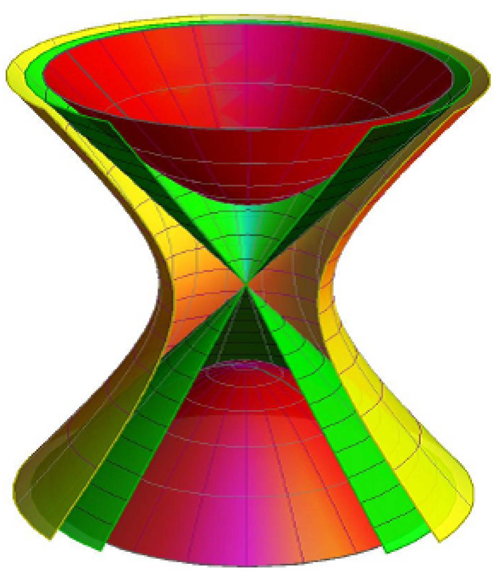
Hence, we have the E. Study map: The ring-shaped hyperboloid represents the set of spacelike lines, the combined asymptotic cone represents the set of null-lines, and the oval-shaped hyperboloid represents the set of timelike lines (see Figure 1). As a consequence, a curve on ${\mathbb{H}}_{+}^2$ matches a timelike ruled surface in $\mathbf{\xi }$${}_1^3$. Additionally, a curve on ${\mathbb{S}}_1^2$ matches a spacelike or timelike ruled surface in ${\mathbb{E}}_1^3$ [8,9,10,11,12,13,14].

Definition 1.

For any two (non-null) dual vectors $\widehat{\mathbf{a}}$ and $\widehat{\mathbf{b}}$ in ${\mathbb{D}}_1^3$, we have [8,9,10,11,12]: (i) If $\widehat{\mathbf{a}}$ and $\widehat{\mathbf{b}}$ are two dual spacelike vectors, then:

• If they span a dual spacelike plane, there is a dual number $\widehat{\theta }=\theta +\epsilon {\theta }^{*}$; $0\le \theta \le \pi$, and ${\theta }^{*}\in \mathbb{R}$ such that $<\widehat{\mathbf{a}},\widehat{\mathbf{b}}>=∥\widehat{\mathbf{a}}∥∥\widehat{\mathbf{b}}∥cos\widehat{\theta }$. This number is the spacelike dual angle amongst $\widehat{\mathbf{a}}$ and $\widehat{\mathbf{b}}$;
• If they span a dual timelike plane, there is a dual number $\widehat{\theta }=\theta +\epsilon {\theta }^{*}\ge 0$ such that $<\widehat{\mathbf{a}},\widehat{\mathbf{b}}>=ϵ∥\widehat{\mathbf{a}}∥∥\widehat{\mathbf{b}}∥cosh\widehat{\theta }$, where $ϵ=+1$ or $ϵ=-1$ via $sign\left({\widehat{a}}_2\right)=sign\left({\widehat{y}}_2\right)$ or $sign\left({\widehat{a}}_2\right)\ne sign\left({\widehat{b}}_2\right)$, respectively. This number is the central dual angle amongst $\widehat{\mathbf{a}}$ and $\widehat{\mathbf{b}}$;
  (ii) If $\widehat{\mathbf{a}}$ and $\widehat{\mathbf{b}}$ are two dual timelike vectors, then there is a dual number $\widehat{\theta }=\theta +\epsilon {\theta }^{*}\ge 0$ such that $<\widehat{\mathbf{a}},\widehat{\mathbf{b}}>=ϵ∥\widehat{\mathbf{a}}∥∥\widehat{\mathbf{b}}∥cosh\widehat{\theta }$, where $ϵ=+1$ or $ϵ=-1$ via $\widehat{\mathbf{a}}$ and $\widehat{\mathbf{b}}$ have different time-direction or the same time-direction, respectively. This dual number is the Lorentzian timelike dual angle amongst $\widehat{\mathbf{a}}$ and $\widehat{\mathbf{b}}$;
  (iii) If $\widehat{\mathbf{a}}$ is dual spacelike, and $\widehat{\mathbf{b}}$ is dual timelike, then there is a dual number $\widehat{\theta }=\theta +\epsilon {\theta }^{*}\ge$ 0 such that $<\widehat{\mathbf{a}},\widehat{\mathbf{b}}>=ϵ∥\widehat{\mathbf{a}}∥∥\widehat{\mathbf{b}}∥sinh\widehat{\theta }$, where $ϵ=+1$ or $ϵ=-1$ via $sign\left({\widehat{a}}_2\right)=sign\left({\widehat{b}}_1\right)$ or $sign\left({\widehat{a}}_2\right)\ne sign\left({\widehat{b}}_1\right)$. This number is the Lorentzian timelike dual angle amongst $\widehat{\mathbf{a}}$ and $\widehat{\mathbf{b}}$.

Definition 2.

A pencil of non-null oriented lines $\widehat{\mathbf{a}}=(\mathbf{a},{\mathbf{a}}^{*})\in {\mathbb{E}}_1^3$ satisfying

$$C:<{\mathbf{a}}^{*},\mathbf{b}>+<{\mathbf{b}}^{*},\mathbf{a}>=0,$$

where ${∥\widehat{\mathbf{b}}∥}^{\mathbf{2}}=\pm 1$ is named a spacelike (timelike) line complex when $<\mathbf{b},{\mathbf{b}}^{*}>\ne 0$. In the special case, C is named a spacelike (timelike) singular line complex if $<{\mathbf{b}}^{*},\mathbf{b}>=0$,and ${∥\widehat{\mathbf{b}}∥}^{\mathbf{2}}=\pm 1$.

A non-null singular line complex is a pencil of all non-null lines $\widehat{\mathbf{a}}$ intersecting the non-null line $\widehat{\mathbf{b}}$. Then, we can have a non-null line congruence by common non-null line complexes. The non-null line congruences include a regular pencil of non-null lines in ${\mathbb{E}}_1^3$ realized as a non-null ruled surface. Non-null ruled surface (such as cone and cylinder ) include non-null lines in which the tangent plane touches the surface over the non-null ruling. Such non-null lines are named non-null torsal lines.

One-Parameter Lorentzian Dual Spherical Movements

Let ${\mathbb{S}}_{1m}^2$ and ${\mathbb{S}}_{1f}^2$ be two Lorentzian dual unit spheres with a joint center $\widehat{\mathbf{0}}$ in ${\mathbb{D}}_1^3$. We choose $\left\{\widehat{\mathbf{\zeta }}\right\}=\{\widehat{\mathbf{0}}$;${\widehat{\mathbf{\zeta }}}_1,{\widehat{\mathbf{\zeta }}}_2,{\widehat{\mathbf{\zeta }}}_3$(timelike)}, and $\left\{\widehat{\mathbf{\xi }}\right\}=\{\widehat{\mathbf{0}}$;${\widehat{\mathbf{\xi }}}_1$,${\widehat{\mathbf{\xi }}}_2$,${\widehat{\mathbf{\xi }}}_3$(timelike)} as two orthonormal dual frames related with ${\mathbb{S}}_{1m}^2$ and ${\mathbb{S}}_{1f}^2$, respectively. If we set $\left\{\widehat{\mathbf{\xi }}\right\}$ is stationary, whereas the components of the set $\left\{\widehat{\mathbf{\zeta }}\right\}$ are functions of a real parameter $t\in \mathbb{R}$ (say the time). Then, we say that ${\mathbb{S}}_{1m}^2$ movements with respect to ${\mathbb{S}}_{1f}^2.$ Such movement is named a one-parameter Lorentzian dual spherical movements, and indicated by ${\mathbb{S}}_{1m}^2/{\mathbb{S}}_{1f}^2$. If ${\mathbb{S}}_{1m}^2$ and ${\mathbb{S}}_{1f}^2$ matches to the Lorentzian line spaces ${\mathbb{L}}_m$ and ${\mathbb{L}}_f$, respectively, then ${\mathbb{S}}_{1m}^2/{\mathbb{S}}_{1f}^2$ matches the one-parameter Lorentzian spatial movements ${\mathbb{L}}_m/{\mathbb{L}}_f.$ Therefore, ${\mathbb{L}}_m$ is the movable Lorentzian space with respect to the invariable Lorentzian space ${\mathbb{L}}_f$ in ${\mathbb{E}}_1^3$. Since each of these orthonormal dual frames has the same direction, one frame is gained by employing second when revolved about $\widehat{\mathbf{0}}$. By letting $<{\widehat{\mathbf{\zeta }}}_i,{\widehat{\mathbf{\xi }}}_j>={\widehat{a}}_{ij}=a_{ij}+\epsilon a_{ij}^{*}$ and considering the dual matrix $\widehat{a}\left(t\right)=\left({\widehat{a}}_{ij}\right)$. It then follows that the signature matrix $ϵ$ of the inner product is specified by

$$ϵ=\left(\begin{array}{ccc}1& 0& 0\\ 0& 1& 0\\ 0& 0& -1\end{array}\right).$$

Hence, the movement ${\mathbb{S}}_{1m}^2/{\mathbb{S}}_{1f}^2$ can be described as

$$\left(\begin{array}{c}{\widehat{\mathbf{\xi }}}_1\hfill \\ {\widehat{\mathbf{\xi }}}_2\hfill \\ {\widehat{\mathbf{\xi }}}_3\hfill \end{array}\right)=\left(\begin{array}{ccc}{\widehat{a}}_{11}\hfill & {\widehat{a}}_{12}\hfill & {\widehat{a}}_{13}\hfill \\ {\widehat{a}}_{21}\hfill & {\widehat{a}}_{22}\hfill & {\widehat{a}}_{23}\hfill \\ {\widehat{a}}_{31}\hfill & {\widehat{a}}_{32}\hfill & {\widehat{a}}_{33}\hfill \end{array}\right)\left(\begin{array}{c}{\widehat{\mathbf{\zeta }}}_1\\ {\widehat{\mathbf{\zeta }}}_2\\ {\widehat{\mathbf{\zeta }}}_3\end{array}\right).$$

Thus, the dual matrix $\widehat{a}\left(t\right)=a_{ij}\left(t\right)+\epsilon a_{ij}^{*}\left(t\right)$ has ${\widehat{a}}^T=ϵ{\widehat{a}}^{-1}ϵ$, and ${\widehat{a}}^{-1}=ϵ{\widehat{a}}^Tϵ$. Therefore, we have:

$$\widehat{a}{\widehat{a}}^{-1}=\widehat{a}ϵ{\widehat{a}}^Tϵa={\widehat{a}}^{-1}\widehat{a}=ϵ{\widehat{a}}^Tϵ\widehat{a}=I,$$

(1)

which mean it is an orthogonal matrix. This outcome indicates that when a one-parameter Lorentzian spatial movement is stated in ${\mathbb{E}}_1^3$, we can locate a Lorentzian dual orthogonal $3\times 3$ matrix $\widehat{a}\left(t\right)=\left({\widehat{a}}_{ij}\right)$, where $\left({\widehat{a}}_{ij}\right)$ are dual functions of one variable $t\in \mathbb{R}$. Similar to the set of real Lorentzian orthogonal matrices, the set of Lorentzian dual orthogonal $3\times 3$ matrices, indicated by $\mathbb{O}\left({\mathbb{D}}_1^{3\times 3}\right)$, locate a group with matrix multiplication as the group operation (real Lorentzian orthogonal matrices are subgroup of Lorentzian dual orthogonal matrices). The identity element of $\mathbb{O}\left({\mathbb{D}}_1^{3\times 3}\right)$ is the $3\times 3$ unit matrix. Since the center of the Lorentzian dual unit sphere in ${\mathbb{D}}_1^3$ should remain inanimate, the transformation group in ${\mathbb{D}}_1^3$ (the picture of Lorentzian movements in the Minkowski 3-space ${\mathbb{E}}_1^3$) does not hold any translations. Then, for the Lorentzian movements in ${\mathbb{D}}_1^3$, we can state the next theorem:

Theorem 1.

The set of all Lorentzian dual orthogonal matrices $\mathbb{O}\left({\mathbb{D}}_1^{3\times 3}\right)$ in ${\mathbb{D}}_1^3$-space is in one-to-one agreement with the set of all one-parameter Lorentzian spatial movements in ${\mathbb{E}}_1^3$-space.

To derive an element of the dual Lie algebra $L\left({\mathbb{O}}_{{\mathbb{D}}_1^{3\times 3}}\right)$ of the dual group $\mathbb{O}\left({\mathbb{D}}_1^{3\times 3}\right)$, we set a Lorentzian dual curve of such dual matrices $\widehat{a}\left(t\right)$ such that $\widehat{a}\left(0\right)$ is the identity. By setting the derivative of Equation (1) with respect to t, we attain:

$${\widehat{a}}^{{}^{\prime }}{\widehat{a}}^{-1}+\widehat{a}{\left({\widehat{a}}^{-1}\right)}^{{}^{\prime }}=0;0\mathrm{is}\mathrm{zero}3\times 3\mathrm{matrix}.$$

If we set $\widehat{\omega }\left(t\right)={\widehat{a}}^{{}^{\prime }}{\widehat{a}}^{-1}$, we see that ${\widehat{\omega }}^T+ϵ\widehat{\omega }ϵ=0$, that is, the matrix $\widehat{\omega }$ is a skew-adjoint matrix. Thus, via Theorem 1, the Lie algebra $L\left({\mathbb{O}}_{{\mathbb{D}}_1^{3\times 3}}\right)$ of the dual Lorentzian group $\mathbb{O}\left({\mathbb{D}}_1^{3\times 3}\right)$ is the algebra of dual skew-adjoint $3\times 3$ matrices

$$\widehat{\omega }\left(t\right):={\widehat{a}}^{{}^{\prime }}ϵ{\widehat{a}}^Tϵ=\left(\begin{array}{ccc}0\hfill & {\widehat{\omega }}_3\hfill & {\widehat{\omega }}_2\hfill \\ -{\widehat{\omega }}_3\hfill & 0\hfill & -{\widehat{\omega }}_1\hfill \\ -{\widehat{\omega }}_2\hfill & -{\widehat{\omega }}_1\hfill & 0\hfill \end{array}\right).$$

(2)

Here, “dash” references the derivative with respect to $t\in \mathbb{R}$. Then,

$$\left(\begin{array}{c}{\widehat{\mathbf{\zeta }}}_1^{{}^{\prime }}\hfill \\ {\widehat{\mathbf{\zeta }}}_2^{{}^{\prime }}\hfill \\ {\widehat{\mathbf{\zeta }}}_3^{{}^{\prime }}\hfill \end{array}\right)=\left(\begin{array}{ccc}0\hfill & {\widehat{\omega }}_3\hfill & {\widehat{\omega }}_2\hfill \\ -{\widehat{\omega }}_3\hfill & 0\hfill & -{\widehat{\omega }}_1\hfill \\ -{\widehat{\omega }}_2\hfill & -{\widehat{\omega }}_1\hfill & 0\hfill \end{array}\right)\left(\begin{array}{c}{\widehat{\mathbf{\zeta }}}_1\\ {\widehat{\mathbf{\zeta }}}_2\\ {\widehat{\mathbf{\zeta }}}_3\end{array}\right)=\widehat{\mathbf{\omega }}\times \left(\begin{array}{c}{\widehat{\mathbf{\zeta }}}_1\\ {\widehat{\mathbf{\zeta }}}_2\\ {\widehat{\mathbf{\zeta }}}_3\end{array}\right),$$

(3)

where $\widehat{\mathbf{\omega }}\left(t\right)=\mathbf{\omega }(t)+\epsilon {\mathbf{\omega }}^{*}\left(t\right)=({\widehat{\omega }}_1,{\widehat{\omega }}_2,{\widehat{\omega }}_3)$ is named the instantaneous dual rotation vector of ${\mathbb{S}}_{1m}^2/{\mathbb{S}}_{1f}^2$. $\mathbf{\omega }$ and ${\mathbf{\omega }}^{*}$, respectively, are the instantaneous rotational differential velocity vector and the instantaneous translational differential velocity vector of the movement ${\mathbb{L}}_m/{\mathbb{L}}_{\xi }$.

3. Timelike Ruled Surfaces with Stationary Disteli-Axis

According to Formula (3), let ${\widehat{\mathbf{\zeta }}}_1\left(t\right)$ be a spacelike dual curve on ${\mathbb{S}}_{1f}^2$ match a timelike ruled surface ($\widehat{\mathbf{\zeta }}$) in ${\mathbb{L}}_f$. As customary Blaschke frame for ${\widehat{\mathbf{\zeta }}}_1\left(t\right)$ will be specified as

$${\widehat{\mathbf{\zeta }}}_1={\widehat{\mathbf{\zeta }}}_1\left(t\right),{\widehat{\mathbf{\zeta }}}_2\left(t\right)={\widehat{\mathbf{\zeta }}}_1^{{}^{\prime }}{∥{\widehat{\mathbf{\zeta }}}_1^{{}^{\prime }}∥}^{-1},{\widehat{\mathbf{\zeta }}}_1\times {\widehat{\mathbf{\zeta }}}_2=-{\widehat{\mathbf{\zeta }}}_3,$$

(4)

where

$$\begin{array}{c}<{\widehat{\mathbf{\zeta }}}_1,{\widehat{\mathbf{\zeta }}}_1>=<{\widehat{\mathbf{\zeta }}}_2,{\widehat{\mathbf{\zeta }}}_2>=1,<{\widehat{\mathbf{\zeta }}}_3,{\widehat{\mathbf{\zeta }}}_3>=-1,\\ {\widehat{\mathbf{\zeta }}}_1\times {\widehat{\mathbf{\zeta }}}_2={\widehat{\mathbf{\zeta }}}_3,{\widehat{\mathbf{\zeta }}}_1\times {\widehat{\mathbf{\zeta }}}_3={\widehat{\mathbf{\zeta }}}_2,{\widehat{\zeta }}_2\times {\widehat{\mathbf{\zeta }}}_3=-{\widehat{\mathbf{\zeta }}}_1.\end{array}$$

The frame $\{{\widehat{\mathbf{\zeta }}}_1\left(t\right),{\widehat{\mathbf{\zeta }}}_2\left(t\right),{\widehat{\mathbf{\zeta }}}_3\left(t\right)\}$ is named Blaschke frame. Through the movement ${\mathbb{S}}_{1m}^2/{\mathbb{S}}_{1f}^2,$ the matching lines intersect at the striction point $\mathbf{c}$ of the ruled surface ($\widehat{\zeta }$). The trajectory of the central points trace the striction curve $\mathbf{c}\left(t\right)$ on ($\widehat{\zeta }$). Therefore, the structural equation of ${\mathbb{S}}_{1m}^2/{\mathbb{S}}_{1f}^2$ is specified by

$$\left(\begin{array}{c}{\widehat{\mathbf{\zeta }}}_1^{{}^{\prime }}\hfill \\ {\widehat{\mathbf{\zeta }}}_2^{{}^{\prime }}\hfill \\ {\widehat{\mathbf{\zeta }}}_3^{{}^{\prime }}\hfill \end{array}\right)=\left(\begin{array}{ccc}0\hfill & \widehat{p}\hfill & 0\hfill \\ -\widehat{p}\hfill & 0\hfill & -\widehat{q}\hfill \\ 0\hfill & -\widehat{q}\hfill & 0\hfill \end{array}\right)\left(\begin{array}{c}{\widehat{\mathbf{\zeta }}}_1\hfill \\ {\widehat{\mathbf{\zeta }}}_2\hfill \\ {\widehat{\mathbf{\zeta }}}_3\hfill \end{array}\right)=\widehat{\mathbf{\omega }}\times \left(\begin{array}{c}{\widehat{\mathbf{\zeta }}}_1\hfill \\ {\widehat{\mathbf{\zeta }}}_2\hfill \\ {\widehat{\mathbf{\zeta }}}_3\hfill \end{array}\right),$$

(5)

where $\widehat{\mathbf{\omega }}\left(t\right)=(\widehat{q},0,\widehat{p})$, and

$$\widehat{p}\left(t\right)=p\left(t\right)+\epsilon p^{*}\left(t\right)=∥{\widehat{\zeta }}_1^{{}^{\prime }}∥,\widehat{q}=q+\epsilon q^{*}=det({\widehat{\mathbf{\zeta }}}_1,{\widehat{\mathbf{\zeta }}}_1^{{}^{\prime }},{\widehat{\mathbf{\zeta }}}_1^{{}^{{}^{″}}}),$$

are the Blaschke invariants of the timelike dual curve $\widehat{\mathbf{r}}\left(t\right)\in {\mathbb{S}}_{1f}^2$. The tangent of the striction curve is:

$${\mathbf{c}}^{{}^{\prime }}\left(t\right)=q^{*}\left(t\right){\mathbf{\zeta }}_1\left(t\right)-p^{*}\left(t\right){\mathbf{\zeta }}_3\left(t\right).$$

(6)

The Lorentzian invariants of ($\widehat{\mathbf{\zeta }}$) are:

$$\gamma \left(t\right)=\frac{q\left(t\right)}{p\left(t\right)},ϝ\left(t\right)=\frac{q^{*}\left(t\right)}{q\left(t\right)},\mathrm{and}\mu \left(t\right)=\frac{p^{*}\left(t\right)}{p\left(t\right)}\mathrm{with}p\left(t\right)\ne 0.$$

(7)

The geometric elucidations of $\gamma \left(t\right)$, $ϝ\left(t\right)$, and $\mu \left(t\right)$ are as follows:$\gamma$ is the spherical curvature of the image curve ${\mathbf{\zeta }}_1(t)$; $ϝ$ is the angle amongst the tangent to the striction curve and the ruling of ($\widehat{\mathbf{\zeta }}$); and $\mu$ is its distribution parameter at the ruling. Thus, a timelike ruled surface can be specified as follows:

$$\left(\widehat{r}\right):\mathbf{y}(t,v)=\stackrel{t}{\underset{0}{\int }}\left(q^{*}\left(t\right){\mathbf{\zeta }}_1\left(t\right)-p^{*}\left(t\right)\mathbf{g}\left(t\right)\right)dt+v{\mathbf{\zeta }}_1\left(t\right).$$

(8)

3.1. Timelike Disteli-Axis

Under the hypothesis that $\left|\widehat{q}\right|<\left|\widehat{p}\right|$, we specify the timelike Disteli-axis of ($\widehat{\mathbf{\zeta }}$) in ${\mathbb{L}}_f$ as follows:

$$\widehat{\mathbf{d}}\left(t\right)=\mathbf{d}\left(t\right)+\epsilon {\mathbf{d}}^{*}\left(t\right)=\frac{\widehat{\mathbf{\omega }}\left(t\right)}{∥\widehat{\mathbf{\omega }}\left(t\right)∥}=\frac{\widehat{q}}{\sqrt{{\widehat{p}}^2-{\widehat{q}}^2}}{\widehat{\mathbf{\zeta }}}_1+\frac{\widehat{p}}{\sqrt{{\widehat{p}}^2-{\widehat{q}}^2}}{\widehat{\mathbf{\zeta }}}_3.$$

(9)

Then, Equation (5) can be written as

$$\left(\begin{array}{c}{\widehat{\mathbf{\zeta }}}_1^{{}^{\prime }}\hfill \\ {\widehat{\mathbf{\zeta }}}_2^{{}^{\prime }}\hfill \\ {\widehat{\mathbf{\zeta }}}_3^{{}^{\prime }}\hfill \end{array}\right)=∥\widehat{\mathbf{\omega }}∥\widehat{\mathbf{d}}\times \left(\begin{array}{c}{\widehat{\mathbf{\zeta }}}_1\hfill \\ {\widehat{\mathbf{\zeta }}}_2\hfill \\ {\widehat{\mathbf{\zeta }}}_3\hfill \end{array}\right).$$

(10)

Therefore, at any instant $t\in \mathbb{R}$, we gain

$${\omega }^{*}\left(t\right)=\frac{p{p}^{*}-q{q}^{*}}{\sqrt{p^2-q^2}},\omega \left(t\right)=\sqrt{p^2-q^2}.$$

Therefore, the timelike Disteli-axis is the instantaneous screw axis of the the movement ${\mathbb{L}}_m/{\mathbb{L}}_f$.

Proposition 1.

The pitch $\beta \left(t\right)$ of the Blaschke frame along the timelike Disteli-axis is specified by

$$\beta \left(t\right):=\frac{<{\mathbf{\omega },\mathbf{\omega }}^{*}>}{{∥\mathbf{\omega }∥}^2}=\frac{p{p}^{*}-q{q}^{*}}{p^2-q^2}.$$

(11)

However, the timelike Disteli-axis $\widehat{\mathbf{d}}\left(t\right)$ can be realized by Equation (9), and we have:

(1) 

The dual angular speed can be specified as $∥\widehat{\mathbf{\omega }}\left(t\right)∥=\omega \left(t\right)(1+\epsilon \beta \left(t\right))$;

(2) 

If $\mathbf{p}(x,y,z)$ be a point on $\widehat{\mathbf{d}}\left(t\right)$, then

$$\mathbf{p}(t,v)=\mathbf{d}\left(t\right)\times {\mathbf{d}}^{*}\left(t\right)+v\mathbf{d}\left(t\right),v\in \mathbb{R}.$$

(12)

is a non-developable timelike ruled surface $\left(\widehat{d}\right)$.

If the movement ${\mathbb{L}}_m/{\mathbb{L}}_f$ is a pure rotation, that is, $\beta \left(t\right)=0$, then,

$$\widehat{\mathbf{d}}\left(t\right)=\mathbf{d}\left(t\right)+\epsilon {\mathbf{d}}^{*}\left(t\right)=\frac{1}{∥\mathbf{\omega }∥}(\mathbf{\omega }+\epsilon {\mathbf{\omega }}^{*}),$$

(13)

whereas, if $\beta \left(t\right)=0$, and ${∥\mathbf{\omega }\left(t\right)∥}^2=1$, then $\widehat{\mathbf{\omega }}\left(t\right)$ is a timelike line. However, if $\widehat{\mathbf{\omega }}\left(t\right)=$0$+\epsilon {\mathbf{\omega }}^{*}\left(t\right)$, that is, the movement ${\mathbb{L}}_m/{\mathbb{L}}_f$ is pure translational, we let ${\omega }^{*}\left(t\right)=∥{\mathbf{\omega }}^{*}\left(t\right)∥;$${\omega }^{*}$d$\left(t\right)={\omega }^{*}$ for arbitrary ${\mathbf{d}}^{*}\left(t\right)$ such that ${\omega }^{*}\left(t\right)\ne 0$, in other view $\mathbf{d}\left(t\right)$ can be arbitrarily selection, too.

Let $\widehat{\varphi }\left(t\right)=\varphi \left(t\right)+\epsilon {\varphi }^{*}\left(t\right)$ be the dual radius of curvature through $\widehat{\mathbf{d}}$ and ${\widehat{\zeta }}_1$ (see Figure 2). Then,

$$\widehat{\mathbf{d}}\left(t\right)=sinh\widehat{\varphi }{\widehat{\mathbf{\zeta }}}_1+cosh\widehat{\varphi }{\widehat{\mathbf{\zeta }}}_3,$$

(14)

where

$$tanh\widehat{\varphi }=tanh\varphi +\epsilon {\varphi }^{*}(1-{tanh}^2\varphi )=\frac{\widehat{q}}{\widehat{p}}.$$

(15)

From Equation (7), (11), and (15), we attain:

$$\left.\begin{array}{c}\beta \left(t\right)=\mu {cosh}^2\varphi -ϝ{sinh}^2\varphi ,\hfill \\ {\varphi }^{*}\left(t\right)=\frac{1}{2}\left(\mu -ϝ\right)sinh2\varphi .\hfill \end{array}\right\}$$

(16)

The first one is due to Hamilton and the second one is due to Mannhiem of surface theory in Euclidean 3-space ${\mathbb{E}}^3$ (Compared with [1,2,3,4]).

3.2. Timelike Plücker’s Conoid

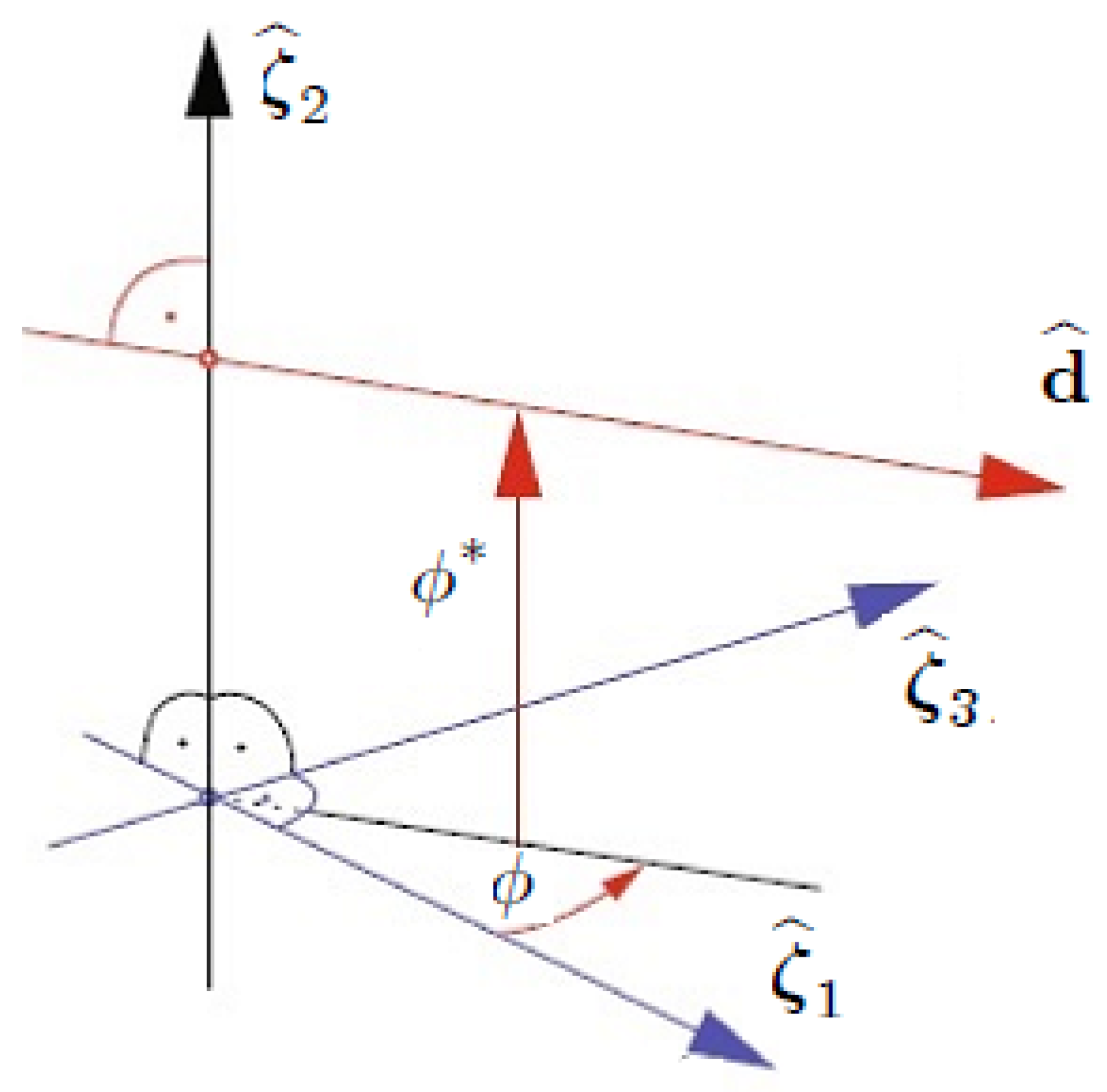
We now explicate and research the geometrical demonstrations of the Hamilton and Mannhiem formulae. The surface defined by ${\varphi }^{*}$ is the timelike form of the well-known Plücker’s conoid, or cylindroid. as follows: let ${\widehat{\mathbf{\zeta }}}_2$ and $y$-axis of a stationary Lorentzian frame $\left(oxyz\right)$ be coincident and the place of the timelike dual unit vector $\widehat{\mathbf{d}}$ be specified by angle $\varphi$ and distance ${\varphi }^{*}$ on the positive orientation of $y-$ axis. The dual unit vectors ${\widehat{\mathbf{\zeta }}}_1$ and ${\widehat{\mathbf{\zeta }}}_3$ can be chosen over the x and z-axes, respectively. This displays that ${\widehat{\mathbf{\zeta }}}_1$ and ${\widehat{\mathbf{\zeta }}}_3$ together with ${\widehat{\mathbf{\zeta }}}_2$ display the coordinate system of the timelike Plücker’s conoid (Figure 2). Therefore, if $\mathbf{r}(x,y,z)$ should be a point on $\left(\widehat{d}\right)$, then we have:

$${\varphi }^{*}:=y=\frac{1}{2}\left(\mu -ϝ\right)sinh2\varphi ,x=vsinh\varphi ,\mathrm{and}z=vcosh\varphi .$$

By an uncomplicated calculation, we gain the algebraic equation

$$\left(\widehat{d}\right):\left(x^2-z^2\right)y+\left(\mu -ϝ\right)xz=0,$$

(17)

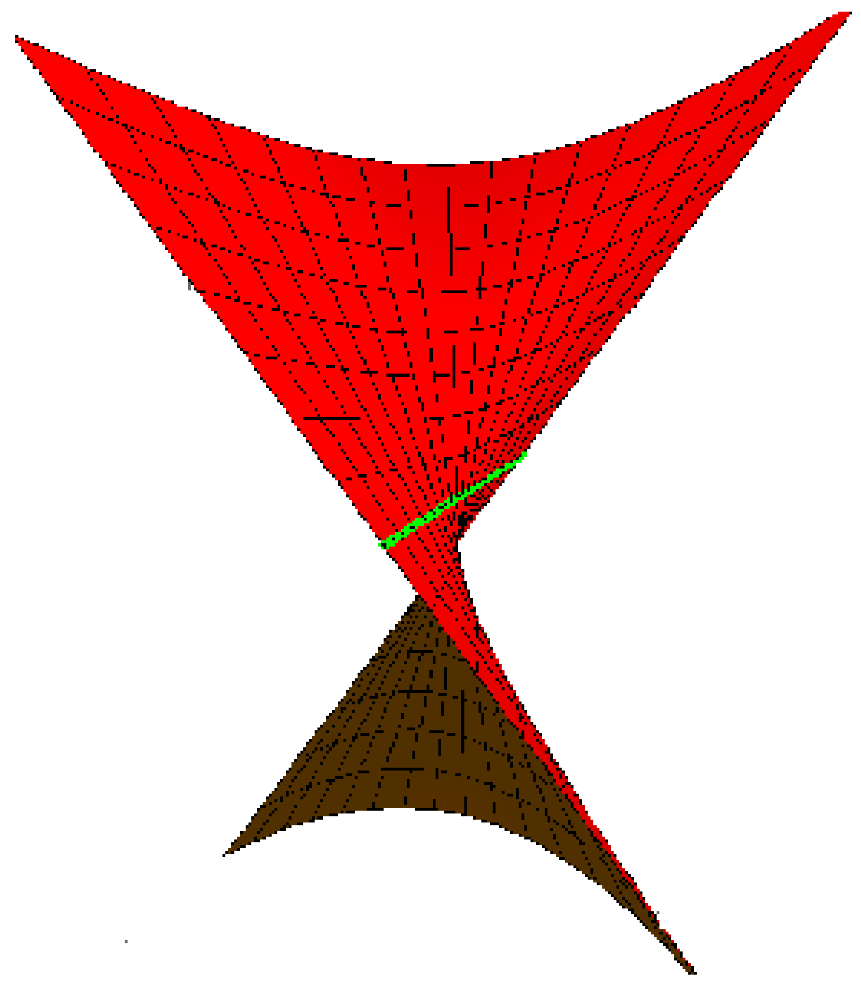
It is clear that Equation (17) depends on the two integral invariants of the first order; $\mu -ϝ=1,0\le \varphi \in \mathbb{R}$, $-2\le \upsilon \le 2$ (Figure 3). Further, one can obtain a second-order algebraic equation in $x/z$ as

$$\frac{x}{z}=\frac{1}{2y}\left[-\left(\mu -ϝ\right)\pm \sqrt{{\left(\mu -ϝ\right)}^2+4y^2}\right].$$

(18)

For the limits of $(\widehat{d}),$ we put ${\left(\mu -ϝ\right)}^2+4y^2=0$. Therefore, the two limits of $(\widehat{d})$ are as follows

$$y=\pm i\left(\mu -ϝ\right)/2,\mathrm{with}i=\sqrt{-1}.$$

(19)

Equation (19) admits two isotropic torsal timelike planes, each of which contains one isotropic torsal timelike line L. Hence, the geometric aspects of the $(\widehat{d})$ are as follows:

(i)

If $\beta \left(t\right)\ne 0$, then we have two generators through the point $(0,y,0)$; and for the two limit isotropic torsal timelike planes $y=\pm i\left(ϝ-\mu \right)/2$, the generators and the principal axes ${\widehat{\mathbf{\zeta }}}_1$ and ${\widehat{\mathbf{\zeta }}}_3$ are coincident;

(ii)

If $\beta \left(t\right)=0,$ then we have two torsal isotropic lines $L_1$, $L_2$ determined by

$$L_1,L_2:\frac{x}{z}=tanh\varphi =\pm \sqrt{\frac{\mu }{ϝ}},y=\pm i\left(\mu -ϝ\right)/2.$$

(20)

Equation (20) offer that the two isotropic torsal lines $L_1$, and $L_2$ are orthogonal to each other. Therefore, if $\mu$ and $ϝ$ are commensurate, then the timelike Plücker’s conoid becomes a pencil of timelike lines in the origin “$\mathbf{o}$” in the timelike torsal plane $y=0$. In this case, $L_1$ and $L_2$ are the principal axes of an elliptic timelike line congruence. However, if $\mu$ and $ϝ$ have opposite signs, then $L_1$ and $L_2$ are isotropic and are coincident with the principal axes of a timelike hyperbolic line congruence.

Furthermore, if we convert from polar coordinates to Cartesian, we use the impersonation

$$x=\frac{1}{\sqrt{\beta }}sinh\varphi ,\mathrm{and}z=\frac{1}{\sqrt{\beta }}cosh\varphi ,$$

into the Hamilton’s formula and we obtain the following conic section

$$D:\left|\mu \right|z^2-\left|ϝ\right|x^2=1.$$

This conic section is a Minkowski version of Dupin’s indicatrix of the surface theory in Euclidean 3-space ${\mathbb{E}}^3$.

Figure 2. $\widehat{\mathbf{d}}=sinh\widehat{\varphi }{\widehat{\mathbf{\zeta }}}_1+cosh\widehat{\varphi }{\widehat{\mathbf{\zeta }}}_3$.

Figure 2. $\widehat{\mathbf{d}}=sinh\widehat{\varphi }{\widehat{\mathbf{\zeta }}}_1+cosh\widehat{\varphi }{\widehat{\mathbf{\zeta }}}_3$.

Figure 3. Timelike Plücker’s conoid.

Figure 3. Timelike Plücker’s conoid.

Serret–Frenet Frame

In Equation (6): (a) If $p^{*}=0$, then $\left(\widehat{\mathbf{\zeta }}\right)$ is a tangential timelike developable surface, that is, ${\mathbf{c}}^{{}^{{}^{\prime }}}=q^{*}{\mathbf{\zeta }}_1$. In this case, the striction curve $\mathbf{c}\left(t\right)$ is a spacelike edge of regression of $\left(\widehat{\mathbf{\zeta }}\right)$, and then D is a pencil of parallel isotropic lines specified by $x=\pm i/$$\left|ϝ\right|$. Let s be an arc-length parameter of $\mathbf{c}\left(t\right)$ and $\{{\mathbf{e}}_1\left(s\right),$${\mathbf{e}}_2\left(s\right)$, ${\mathbf{e}}_3\left(s\right);\kappa \left(s\right)$, $\tau \left(s\right)\}$ is the Serret–Frenet apparatus of $\mathbf{c}\left(t\right)$. After several algebraic manipulations, it can be gained that:

$$\frac{d}{ds}\left(\begin{array}{c}{\mathbf{e}}_1\hfill \\ {\mathbf{e}}_2\hfill \\ {\mathbf{e}}_3\hfill \end{array}\right)=\left(\begin{array}{ccc}0\hfill & \kappa \hfill & 0\hfill \\ -\kappa \hfill & 0\hfill & -\tau \hfill \\ 0\hfill & -\tau \hfill & 0\hfill \end{array}\right)\left(\begin{array}{c}{\mathbf{e}}_1\hfill \\ {\mathbf{e}}_2\hfill \\ {\mathbf{e}}_3\hfill \end{array}\right),$$

where

$$\kappa \left(s\right)=\frac{p}{q^{*}},\tau \left(s\right)=\frac{1}{ϝ},\mathrm{with}{q}^{*}\ne 0.$$

Therefore, the curvature function $ϝ\left(s\right)$ is the radius of torsion of the spacelike striction curve $\mathbf{c}\left(s\right)$. Further, we therefore arrive at:

$$\left.\begin{array}{c}\beta \left(s\right)=-\frac{1}{\tau }{sinh}^2\varphi ,{\varphi }^{*}\left(s\right)=-\frac{1}{2\tau }sinh2\varphi ,\hfill \\ \left(\widehat{d}\right):\left(x^2-z^2\right)y-\frac{1}{\tau }xz=0.\hfill \end{array}\right\}$$

(b) If $q^{*}\left(t\right)=0$, the striction curve is timelike tangent to ${\mathbf{\zeta }}_3$; it is normal to rule over $\mathbf{c}\left(t\right)$. In this case, $\left(\widehat{\mathbf{\zeta }}\right)$ is a binormal timelike ruled surface, and D is a pencil of parallel lines decided by $z=\pm 1/$$\left|\mu \right|$. Similarly, we can also specify that:

$$\kappa \left(s\right)=\frac{q\left(s\right)}{p^{*}\left(s\right)},\mathrm{and}\tau \left(s\right)=\frac{1}{\mu \left(s\right)},\mathrm{with}{p}^{*}\left(s\right)\ne 0.$$

Then, the curvature function $\mu \left(s\right)$ is the radius of torsion of $\mathbf{c}\left(s\right)$ of the timelike binormal surface $\left(\widehat{\zeta }\right)$. Additionally, we derive

$$\left.\begin{array}{c}\beta \left(s\right)=\frac{1}{\tau }{cosh}^2\varphi ,{\varphi }^{*}\left(s\right)=\frac{1}{2\tau \left(s\right)}sinh2\varphi ,\hfill \\ \left(\widehat{d}\right):\left(x^2-z^2\right)y+\frac{1}{\tau }xz=0.\hfill \end{array}\right\}$$

3.3. Stationary Timelike Disteli-Axis

In what follow, when we state that ($\widehat{\mathbf{\zeta }}$) is a timelike ruled surface with stationary timelike Disteli-axis, we mean that all the rulings of ($\widehat{\mathbf{\zeta }}$) have a stationary dual angle with respect the Disteli-axis.

Let $d\widehat{s}=ds+\epsilon d{s}^{*}$ indicate the dual arc length of ${\widehat{\mathbf{\zeta }}}_1\left(t\right)$ Then,

$$\widehat{s}\left(t\right)=\stackrel{t}{\underset{0}{\int }}\widehat{p}dt=\stackrel{t}{\underset{0}{\int }}p(1+\epsilon \mu )dt.$$

(21)

By employing $\widehat{s}$ instead of t, from Equations (5) and (21), we have:

$$\left(\begin{array}{c}{\widehat{\mathbf{\zeta }}}_1^{{}^{\prime }}\hfill \\ {\widehat{\mathbf{\zeta }}}_2^{{}^{\prime }}\hfill \\ {\widehat{\mathbf{\zeta }}}_3^{{}^{\prime }}\hfill \end{array}\right)=\left(\begin{array}{ccc}0\hfill & 1\hfill & 0\hfill \\ -1\hfill & 0\hfill & -\widehat{\chi }\hfill \\ 0\hfill & -\widehat{\chi }\hfill & 0\hfill \end{array}\right)\left(\begin{array}{c}{\widehat{\mathbf{\zeta }}}_1\hfill \\ {\widehat{\mathbf{\zeta }}}_2\hfill \\ {\widehat{\mathbf{\zeta }}}_3\hfill \end{array}\right)=\widehat{\mathbf{\omega }}\times \left(\begin{array}{c}{\widehat{\mathbf{\zeta }}}_1\hfill \\ {\widehat{\mathbf{\zeta }}}_2\hfill \\ {\widehat{\mathbf{\zeta }}}_3\hfill \end{array}\right);(\prime =\frac{d}{d\widehat{s}}),$$

(22)

where $\widehat{\mathbf{\omega }}\left(\widehat{s}\right)=(\widehat{\chi },0,1)$, $\widehat{\chi }\left(\widehat{s}\right):=\chi +\epsilon {\chi }^{*}=\frac{\widehat{q}}{\widehat{p}}$ is the dual spherical curvature of ${\widehat{\mathbf{\zeta }}}_1\left(\widehat{s}\right)\in {\mathbb{S}}_{1f}^2$. Therefore, we have the following associations:

$$\left.\begin{array}{c}\widehat{\gamma }\left(\widehat{s}\right)=\gamma +\epsilon \left(ϝ-\chi \mu \right)=tanh\widehat{\varphi },\hfill \\ \widehat{\kappa }\left(\widehat{s}\right):=\kappa +\epsilon {\kappa }^{*}=\sqrt{1-{\widehat{\chi }}^2}=\frac{1}{cosh\widehat{\varphi }}=\frac{1}{\widehat{\rho }\left(\widehat{s}\right)},\hfill \\ \widehat{\tau }\left(\widehat{s}\right):=\tau +\epsilon {\tau }^{*}=\pm {\widehat{\varphi }}^{{}^{\prime }}=\pm \frac{{\widehat{\chi }}^{{}^{\prime }}}{1-{\widehat{\chi }}^2}.\hfill \end{array}\right\}$$

(23)

where $\widehat{\kappa }\left(\widehat{s}\right)$ is the dual curvature, and $\widehat{\tau }\left(\widehat{s}\right)$ is the dual torsion of the dual curve ${\widehat{\mathbf{\zeta }}}_1\in {\mathbb{S}}_{1\xi }^2$.

3.3.1. Height Dual Functions

In identification with [17,18], a dual point ${\widehat{\mathbf{d}}}_0$ of $\mathbb{S}$${}_{1f}^2$ will be named a ${\widehat{\mathbf{d}}}_k$ evolute of the dual curve ${\widehat{\mathbf{\zeta }}}_1\left(\widehat{s}\right)\in \mathbb{S}$${}_{1f}^2$; for all t such that $1\le t\le k$, $<{\widehat{\mathbf{d}}}_0,{\widehat{\mathbf{\zeta }}}_1^t\left(\widehat{s}\right)>=0$, but $<{\widehat{\mathbf{d}}}_0,{\widehat{\mathbf{\zeta }}}_1^{k+1}\left(\widehat{s}\right)>\ne 0$. Here ${\widehat{\mathbf{\zeta }}}_1^t$ indicates the t-th derivatives of ${\widehat{\mathbf{\zeta }}}_1$ with respect to the dual arc length $\widehat{s}$. For the first evolute $\widehat{\mathbf{d}}$ of ${\widehat{\mathbf{\zeta }}}_1\left(\widehat{s}\right)$, we have $<\widehat{\mathbf{d}},{\widehat{\mathbf{\zeta }}}_1^{{}^{\prime }}>=\pm <\widehat{\mathbf{d}},{\widehat{\mathbf{\zeta }}}_2>=0$, and $<\widehat{\mathbf{d}},{\widehat{\mathbf{\zeta }}}_1^{{}^{″}}>=\pm <\widehat{\mathbf{d}},{\widehat{\mathbf{\zeta }}}_1+\widehat{\chi }{\widehat{\mathbf{\zeta }}}_3>\ne 0$. Therefore, $\widehat{\mathbf{d}}$ is at least a ${\widehat{\mathbf{d}}}_2$ evolute of ${\widehat{\mathbf{\zeta }}}_1\left(\widehat{s}\right)\in \mathbb{S}$${}_{1f}^2$.

We are now heading a dual function $\widehat{f}:I\times {\mathbb{S}}_{1f}^2\to \mathbb{D}$, by $\widehat{f}(\widehat{s},{\widehat{\mathbf{d}}}_0)=<{\widehat{\mathbf{d}}}_0,{\widehat{\mathbf{\zeta }}}_1>$. We call $\widehat{f}$ a Lorentzian height dual function on ${\widehat{\mathbf{\zeta }}}_1\left(\widehat{s}\right)\in \mathbb{S}$${}_{1f}^2$. We use the notation $\widehat{f}\left(\widehat{s}\right)=\widehat{f}(\widehat{s},{\widehat{\mathbf{d}}}_0)$ for any stationary point ${\widehat{\mathbf{d}}}_0\in \mathbb{S}$${}_{1f}^2$.

Proposition 2.

Under the above notations, the following holds:

1. 

$\widehat{f}$ will be stationary in the first approximation iff ${\widehat{\mathbf{d}}}_0\in Sp\{{\widehat{\mathbf{\zeta }}}_1$,${\widehat{\mathbf{\zeta }}}_3\}$, that is,

$${\widehat{f}}^{{}^{\prime }}=0\iff <{\widehat{\mathbf{\zeta }}}_1^{{}^{\prime }},{\widehat{\mathbf{d}}}_0>=0\iff <{\widehat{\mathbf{\zeta }}}_2,{\widehat{\mathbf{d}}}_0>=0\iff {\widehat{\mathbf{d}}}_0={\widehat{a}}_1{\widehat{\mathbf{\zeta }}}_1+{\widehat{a}}_3{\widehat{\mathbf{\zeta }}}_3;$$

for some dual numbers ${\widehat{a}}_1,{\widehat{a}}_3\in \mathbb{D},$ and ${\widehat{a}}_1^2-{\widehat{a}}_3^2=1$;

2. 

$\widehat{f}$ will be stationary in the second approximation iff ${\widehat{\mathbf{d}}}_0$ is ${\widehat{\mathbf{d}}}_2$ evolute of ${\widehat{\mathbf{d}}}_0\in \mathbb{S}$${}_{1f}^2$, that is,

$${\widehat{f}}^{{}^{\prime }}={\widehat{f}}^{{}^{″}}=0\iff {\widehat{\mathbf{d}}}_0=\pm \widehat{\mathbf{d}}.$$

;

3. 

$\widehat{f}$ will be invariant in the third approximation iff ${\widehat{\mathbf{d}}}_0$ is ${\widehat{\mathbf{d}}}_3$ evolute of ${\widehat{\mathbf{d}}}_0\in$$\mathbb{S}$${}_{1f}^2$, that is,

$${\widehat{f}}^{{}^{\prime }}={\widehat{f}}^{{}^{″}}={\widehat{f}}^{{}^{‴}}=0\iff {\widehat{\mathbf{d}}}_0=\pm \widehat{\mathbf{d}},\mathrm{and}{\widehat{\chi }}^{{}^{\prime }}\ne 0.$$

;

4. 

$\widehat{f}$ will be stationary in the fourth approximation iff ${\widehat{\mathbf{d}}}_0$ is ${\widehat{\mathbf{d}}}_4$ evolute of ${\widehat{\mathbf{d}}}_0\in \mathbb{S}$${}_{1f}^2$, that is,

$${\widehat{f}}^{{}^{\prime }}={\widehat{f}}^{{}^{″}}={\widehat{f}}^{{}^{‴}}={\widehat{f}}^{iv}=0\iff {\widehat{\mathbf{d}}}_0=\pm \widehat{\mathbf{d}},{\widehat{\chi }}^{{}^{\prime }}=0,\mathrm{and}{\widehat{\gamma }}^{{}^{″}}\ne 0.$$

Proof. 

For the first derivative of $\widehat{f}$ we obtain:

$${\widehat{f}}^{{}^{\prime }}=<{\widehat{\mathbf{\zeta }}}_1^{{}^{\prime }},{\widehat{\mathbf{d}}}_0>.$$

(24)

Therefore, we obtain:

$${\widehat{f}}^{{}^{\prime }}=0\iff <{\widehat{\mathbf{\zeta }}}_2,{\widehat{\mathbf{d}}}_0>=0\iff {\widehat{\mathbf{d}}}_0={\widehat{a}}_1{\widehat{\mathbf{\zeta }}}_1+{\widehat{a}}_2{\widehat{\mathbf{\zeta }}}_3;$$

(25)

for some dual numbers ${\widehat{a}}_1,$${\widehat{a}}_2\in \mathbb{D},$ and ${\widehat{a}}_1^2-{\widehat{a}}_3^2=1$, the result is clear.

2-Derivative of Equation (24) leads to:

$${\widehat{f}}^{{}^{″}}=<{\widehat{\mathbf{\zeta }}}_1^{{}^{{}^{″}}},{\widehat{\mathbf{d}}}_0>=-<{\widehat{\mathbf{\zeta }}}_1+\widehat{\chi }{\widehat{\mathbf{\zeta }}}_3,{\widehat{\mathbf{d}}}_0>.$$

(26)

By the Equations (24) and (26) we have:

$${\widehat{f}}^{{}^{\prime }}={\widehat{f}}^{{}^{″}}=0\iff <{\widehat{\mathbf{\zeta }}}_1^{{}^{\prime }},{\widehat{\mathbf{d}}}_0>=<{\widehat{\mathbf{\zeta }}}_1^{{}^{{}^{″}}},{\widehat{\mathbf{d}}}_0>=0\iff {\widehat{\mathbf{d}}}_0=\pm \frac{{\widehat{\mathbf{\zeta }}}_1^{{}^{\prime }}\times {\widehat{\mathbf{\zeta }}}_1^{{}^{{}^{″}}}}{∥{\widehat{\mathbf{\zeta }}}_1^{{}^{\prime }}\times {\widehat{\mathbf{\zeta }}}_1^{{}^{{}^{″}}}∥}=\pm \widehat{\mathbf{d}}.$$

(27)

3-Derivative of Equation (26) leads to:

$${\widehat{f}}^{{}^{‴}}=<{\widehat{\mathbf{x}}}^{{}^{‴}},{\widehat{\mathbf{d}}}_{\mathbf{0}}>=-\left(1+{\widehat{\chi }}^2\right)<{\widehat{\mathbf{\zeta }}}_2,{\widehat{\mathbf{d}}}_0>-{\widehat{\chi }}^{{}^{\prime }}<\widehat{\mathbf{g}},{\widehat{\mathbf{d}}}_0>$$

(28)

Hence, we have:

$${\widehat{f}}^{{}^{\prime }}={\widehat{f}}^{{}^{″}}={\widehat{f}}^{{}^{‴}}=0\iff {\widehat{\mathbf{d}}}_0=\pm \widehat{\mathbf{d}},\mathrm{and}{\widehat{\chi }}^{{}^{\prime }}\ne 0.$$

(29)

4-By the similar arguments, we can also have:

$${\widehat{f}}^{{}^{\prime }}={\widehat{f}}^{{}^{″}}={\widehat{f}}^{{}^{‴}}={\widehat{f}}^{{}^{⁗}}=0\iff {\widehat{\mathbf{d}}}_0=\pm \widehat{\mathbf{d}},{\widehat{\chi }}^{{}^{\prime }}=0,\mathrm{and}{\widehat{\chi }}^{{}^{″}}\ne 0.$$

(30)

The proof is completed. □

(a)

The osculating circle $\mathbb{S}(\widehat{\rho },{\widehat{\mathbf{d}}}_0)$ of ${\widehat{\mathbf{\zeta }}}_1\left(\widehat{s}\right)$ in ${\mathbb{S}}_{1f}^2$ is specified by

$$<{\widehat{\mathbf{d}}}_0{,\widehat{\mathbf{\zeta }}}_1>=\widehat{\rho }\left(\widehat{s}\right),{<\widehat{\mathbf{\zeta }}}_1^{\prime },{\widehat{\mathbf{d}}}_0>=0,{<\widehat{\mathbf{\zeta }}}_1^{{}^{{}^{″}}},{\widehat{\mathbf{d}}}_0>=0,$$

which are gained from the condition that the osculating circle must have touch of at least third order at ${\widehat{\mathbf{\zeta }}}_1\left({\widehat{s}}_0\right)$ if and only if ${\widehat{\chi }}^{{}^{\prime }}\ne 0$.

(b)

The osculating circle $\mathbb{S}(\widehat{\rho },{\widehat{\mathbf{d}}}_0)$ and the curve ${\widehat{\mathbf{\zeta }}}_1\left(\widehat{s}\right)$ in $\mathbb{S}$${}_{1f}^2$ have at least fourth order at ${\widehat{\mathbf{\zeta }}}_1\left(s_0\right)$ if and only if ${\widehat{\chi }}^{{}^{\prime }}=0$, and ${\widehat{\chi }}^{{}^{″}}\ne 0$.

In this direction, by catching into contemplation the evolutes of ${\widehat{\mathbf{\zeta }}}_1\left(\widehat{s}\right)$ in $\mathbb{S}$${}_{1f}^2$, we can gain a sequence of evolutes ${\widehat{\mathbf{d}}}_2$, ${\widehat{\mathbf{d}}}_3$, …, ${\widehat{\mathbf{d}}}_n$. The ownerships and the interrelatedness through these evolutes and their involutes are very interesting problems. For instance, it is not difficult to consider that when ${\widehat{\mathbf{d}}}_0=\pm \widehat{\mathbf{d}}$, and ${\widehat{\chi }}^{{}^{\prime }}=0$, ${\widehat{\mathbf{\zeta }}}_1\left(\widehat{s}\right)$ is situated at $\widehat{\varphi }$ is invariable relative to ${\widehat{\mathbf{d}}}_0$. In this case, the timelike Disteli-axis is invariable up to second order, and the line ${\widehat{\mathbf{\zeta }}}_1$ moves over it with invariable pitch. Thus, the timelike ruled surface ($\widehat{\mathbf{\zeta }}$) with invariable timelike Disteli-axis is produced by timelike line ${\widehat{\mathbf{\zeta }}}_1$ existing at a Lorentzian invariable distance ${\varphi }^{*}$ and Lorentzian invariable angle $\varphi$ with respect to the timelike Disteli-axis $\widehat{\mathbf{d}}$. In the case of $\widehat{\chi }\left(\widehat{s}\right)=0$, then ${\widehat{\mathbf{\zeta }}}_1\left(\widehat{s}\right)$ is a spacelike dual great circle on ${\mathbb{S}}_{1f}^2$, that is,

$$\widehat{c}=\{{\widehat{\mathbf{\zeta }}}_1\in {\mathbb{S}}_{1f}^2\mid <{\widehat{\mathbf{\zeta }}}_1,\widehat{\mathbf{d}}>=0;\mathrm{with}{∥\widehat{\mathbf{d}}∥}^2=-1\}.$$

In this case, in the Lorentzian sense, all the spacelike rulings of ($\widehat{\mathbf{\zeta }}$) intersected orthogonally with the timelike Disteli-axis $\widehat{\mathbf{d}}$, that is, $\varphi =0$, and ${\varphi }^{*}=0$. Thus, we have $\widehat{\chi }\left(\widehat{s}\right)=0\iff$($\widehat{\zeta }$) is a timelike helicoid of the first kind.

Theorem 2.

A non-developable timelike ruled surface $\left(\widehat{\zeta }\right)$ is a stationary timelike Disteli-axis iff $\chi \left(s\right)$ = invariable, and $ϝ\left(s\right)-\chi \left(s\right)\mu \left(s\right)$=invariable.

However, from the Equation ((22)) we have the ODE ${\widehat{\mathbf{\zeta }}}_1^{{}^{{}^{‴}}}+{\widehat{\kappa }}^2{\widehat{\mathbf{\zeta }}}_1^{{}^{\prime }}=\mathbf{0}$. After several algebraic manipulations, the general solution of this equation is:

$${\widehat{\mathbf{\zeta }}}_1\left(\widehat{\phi }\right)=\left(cosh\widehat{\varphi }sin\widehat{\phi },-cosh\widehat{\varphi }cos\widehat{\phi },sinh\widehat{\varphi }\right).$$

(31)

Here, $\widehat{\kappa }\widehat{s}=\widehat{\phi }\left(\widehat{s}\right):=\phi +\epsilon {\phi }^{*}$; where $0\le \phi \le 2\pi$, and ${\phi }^{*}\in \mathbb{R}$. From the real and the dual parts, we have

$$\left.\begin{array}{c}{\zeta }_1=cosh\varphi sin\phi ,{\zeta }_1^{*}={\varphi }^{*}sinh\varphi sin\phi +{\phi }^{*}cosh\varphi cos\phi ,\hfill \\ {\zeta }_2=-cosh\varphi cos\phi ,{\zeta }_2^{*}=-{\varphi }^{*}sinh\varphi cos\phi +{\phi }^{*}cosh\varphi sin\phi ,\hfill \\ {\zeta }_3=sinh\varphi ,{\zeta }_3^{*}={\varphi }^{*}cosh\varphi .\hfill \end{array}\right\}$$

(32)

Let p$(p_1,p_2,p_3)$ be a point on ${\widehat{\mathbf{\zeta }}}_1$. Since ${\zeta }_1^{*}$=p×${\zeta }_1$ we have the system of linear equations in $p_i$(i = 1, 2, 3, and $p_{is}$ are the coordinates of p):

$$\left.\begin{array}{c}{p}_{2}sinh\varphi +p_{3}cosh\varphi cos\phi ={\zeta }_1^{*},\\ -p_{1}sinh\varphi +p_{3}cosh\varphi sin\phi ={\zeta }_2^{*},\\ p_{1}cosh\varphi cos\phi +p_{2}cosh\varphi sin\phi ={\zeta }_3^{*}.\end{array}\right\}$$

(33)

The matrix of coefficients of unknowns $p_i$ is the skew symmetric matrix

$$\left(\begin{array}{ccc}0\hfill & sinh\varphi \hfill & cosh\varphi cos\phi \hfill \\ -sinh\varphi \hfill & 0\hfill & cosh\varphi sin\phi \hfill \\ cosh\varphi cos\phi \hfill & cosh\varphi sin\phi \hfill & 0\hfill \end{array}\right),$$

and thus its rank is 2 with $\varphi \ne 2\pi k$ (k is an integer). The rank of the augmented matrix

$$\left(\begin{array}{cccc}0\hfill & sinh\varphi \hfill & cosh\varphi cos\phi \hfill & {\zeta }_1^{*}\\ -sinh\varphi \hfill & 0\hfill & cosh\varphi sin\phi \hfill & {\zeta }_2^{*}\\ cosh\varphi cos\phi \hfill & cosh\varphi sin\phi \hfill & 0\hfill & {\zeta }_2^{*}\end{array}\right),$$

is also 2. Then, this system has infinite solutions given by

$$\begin{array}{c}{p}_{1}cos\phi +p_{2}sin\phi ={\varphi }^{*}\\ p_1=(p_3-{\varphi }^{*})coth\varphi sin\phi +{\varphi }^{*}cos\phi ,\\ p_2=-(p_3-{\varphi }^{*})coth\varphi cos\phi +{\varphi }^{*}sin\phi .\end{array}$$

(34)

Since $p_3$ can be arbitrarily, then we may put $p_3={\phi }^{*}$. In this case, the Equation ((34)) becomes

$$p_1={\varphi }^{*}cos\phi ,p_2={\varphi }^{*}sin\phi ,p_3={\phi }^{*}.$$

(35)

Thus, the director surface of the timelike congruence is:

$$\mathbf{p}({\varphi }^{*},\varphi )=({\varphi }^{*}cos\phi ,{\varphi }^{*}sin\phi ,{\phi }^{*})$$

Let y$(y_1,y_2,y_3)$ be a point on this timelike congruence. Hence, we obtain:

$$\left(\widehat{\zeta }\right):\mathbf{y}(\phi ,{\phi }^{*}v)=\left(\begin{array}{c}{\varphi }^{*}cos\phi +vcosh\varphi sin\phi \\ {\varphi }^{*}sin\phi -vcosh\varphi cos\phi \\ {\phi }^{*}+vsinh\varphi \end{array}\right),v\in \mathbb{R}.$$

(36)

All lines which satisfy the Equation (36) is a timelike congruence. Also, we may write that

$$\left(\widehat{\zeta }\right):\frac{y_1^2}{{\varphi }^{*2}}+\frac{y_2^2}{{\varphi }^{*2}}-\frac{Y_3^2}{{\Delta }^2}=1,$$

(37)

where $\Delta ={\varphi }^{*}tanh\varphi$, and $Y_3=y_3-{\phi }^{*}$. Then $\left(\widehat{\zeta }\right)$ is a one-parameter family of Lorentzian spheres. The common of each Lorentzian sphere and the conformable spacelike plane $y_3={\phi }^{*}$ is a one-parameter family of Lorentzian cylinders $\left(c\right)$: $y_1^2+y_2^2={\varphi }^{*2}$. Therefore, the envelope of $\left(\widehat{\zeta }\right)$ is the Lorentzian cylinder which is the position for ${\varphi }^{*}=\varphi =0$.

3.3.2. Special Timelike Ruled Surfaces

A correlation such as $\mathsf{\Gamma }(\phi ,{\phi }^{*})=0$ restricts the Equations (36) and (37) to a 1-parameter set of timelike lines, that is, a timelike ruled surface in the line congruence. Therefore, if we set ${\phi }^{*}=\beta \phi ,$$\beta$ indicating the pitch of the movement ${\mathbb{L}}_m/{\mathbb{L}}_f$ and $\phi$ as the movement parameter, then Equations (36) and (37) is a timelike ruled surface in ${\mathbb{L}}_f$-space. Thus, from the Equations (4) and (31), we immediately find that:

$$\left(\begin{array}{c}{\widehat{\mathbf{\zeta }}}_1\hfill \\ {\widehat{\mathbf{\zeta }}}_2\hfill \\ {\widehat{\mathbf{\zeta }}}_3\hfill \end{array}\right)=\left(\begin{array}{ccc}cosh\widehat{\varphi }sin\widehat{\phi }\hfill & -cosh\widehat{\varphi }cos\widehat{\phi }\hfill & sinh\widehat{\varphi }\hfill \\ cos\widehat{\phi }\hfill & sin\widehat{\phi }\hfill & 0\hfill \\ -sinh\widehat{\varphi }sin\widehat{\phi }\hfill & sinh\widehat{\varphi }cos\widehat{\phi }\hfill & -cosh\widehat{\varphi }\hfill \end{array}\right)\left(\begin{array}{c}{\widehat{\mathbf{\xi }}}_1\hfill \\ {\widehat{\mathbf{\xi }}}_2\hfill \\ {\widehat{\mathbf{\xi }}}_3\hfill \end{array}\right).$$

(38)

From the Equations (14) and (38), we have:

$$\widehat{\mathbf{d}}=sinh\widehat{\varphi }{\widehat{\mathbf{\zeta }}}_1+cosh\widehat{\varphi }{\widehat{\mathbf{\zeta }}}_3={\widehat{\mathbf{\xi }}}_3.$$

(39)

This insist that the timelike Disteli-axis $\widehat{\mathbf{d}}$ is ${\widehat{\mathbf{\xi }}}_3$. Additionally, the director surface of the timelike congruence reduces to the striction curve, that is,

$$\mathbf{c}\left(\phi \right)=({\varphi }^{*}cos\phi ,{\varphi }^{*}sin\phi ,h\phi ).$$

It can be shown that $\mathbf{c}\left(\phi \right)$ is a spacelike (a timelike) if and only if $\left|{\varphi }^{*}\right|>\left|h\right|$($\left|{\varphi }^{*}\right|<\left|h\right|$). Further, the curvature ${\kappa }_c\left(\phi \right)$ and torsion ${\tau }_c\left(\phi \right)$ can be specified by

$${\kappa }_c\left(\phi \right)=\frac{{\varphi }^{*}}{{\varphi }^{*2}-h^2},{\tau }_c\left(\phi \right)=\frac{h}{{\varphi }^{*2}-h^2}.$$

Then, $\mathbf{c}\left(\phi \right)$ is a spacelike or timelike helix. Additionally, the timelike ruled surface $\left(\widehat{\zeta }\right)$ with stationary timelike Disteli-axis is:

$$\left(\widehat{\zeta }\right):\mathbf{y}(\phi ,v)=\left(\begin{array}{c}{\varphi }^{*}cos\phi +vcosh\varphi sin\phi \\ {\varphi }^{*}sin\phi -vcosh\varphi cos\phi \\ \beta \phi +vsinh\varphi \end{array}\right),v\in \mathbb{R}.$$

(40)

$\beta$, $\varphi$ and ${\varphi }^{*}$ can control the shape of $\left(\widehat{\zeta }\right)$, that is, it can be classified into the following:

(1)

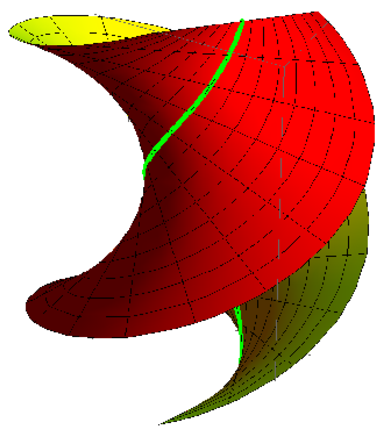
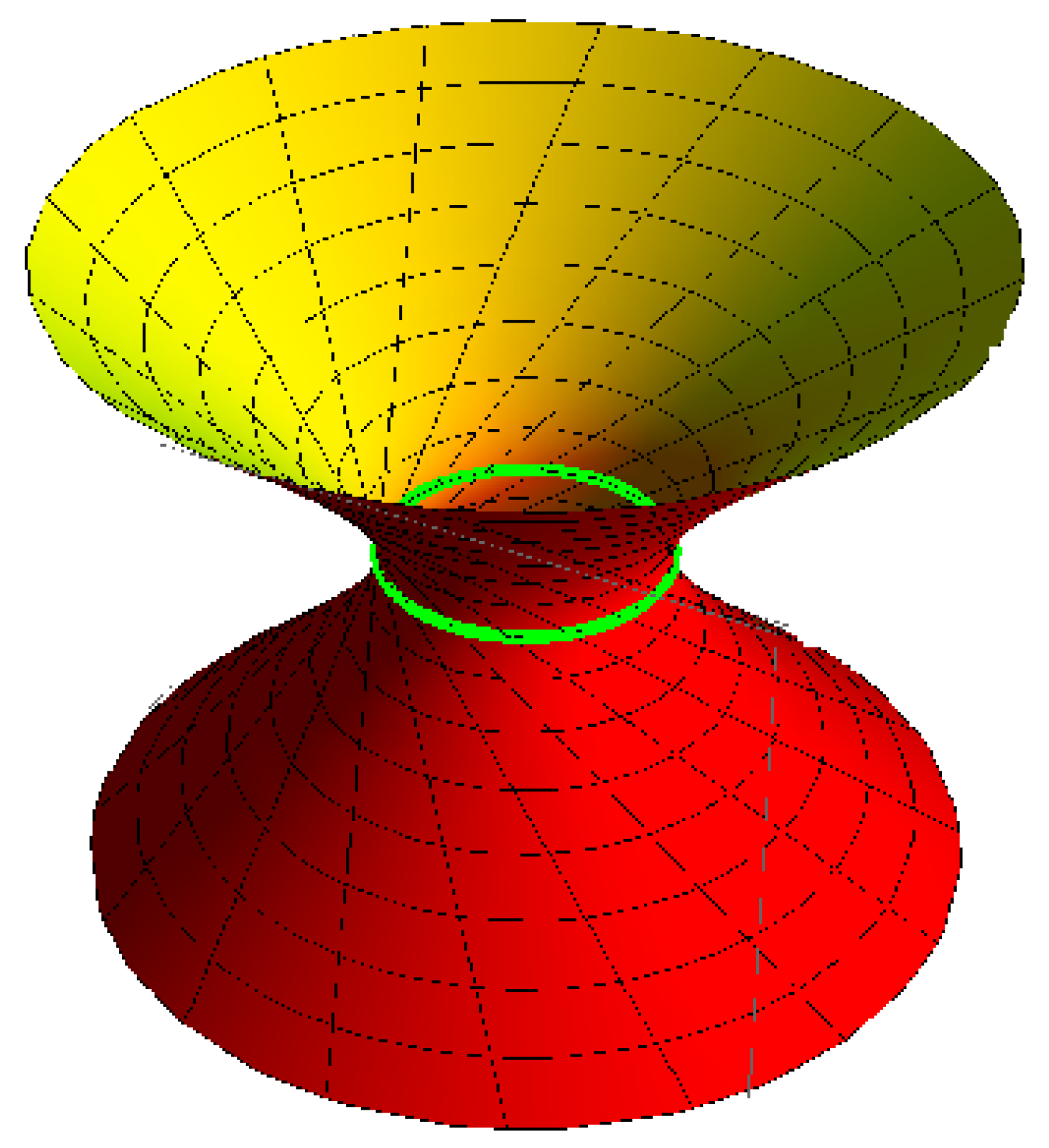
General timelike helicoidal surface with its striction curve is a timelike cylindrical helix: for $\beta =1.5$, ${\varphi }^{*}=1$, $\varphi =0.5$, $-3\le v\le 3$ and $0\le \phi \le 2\pi$ (see Figure 4).

(2)

Lorentzian sphere with its striction curve is a spacelike circle: for $\beta =0,$${\varphi }^{*}=1$, $\varphi =1.3$, $-1.5\le v\le 1.5$, and $0\le \phi \le 2\pi$ (see Figure 5).

(3)

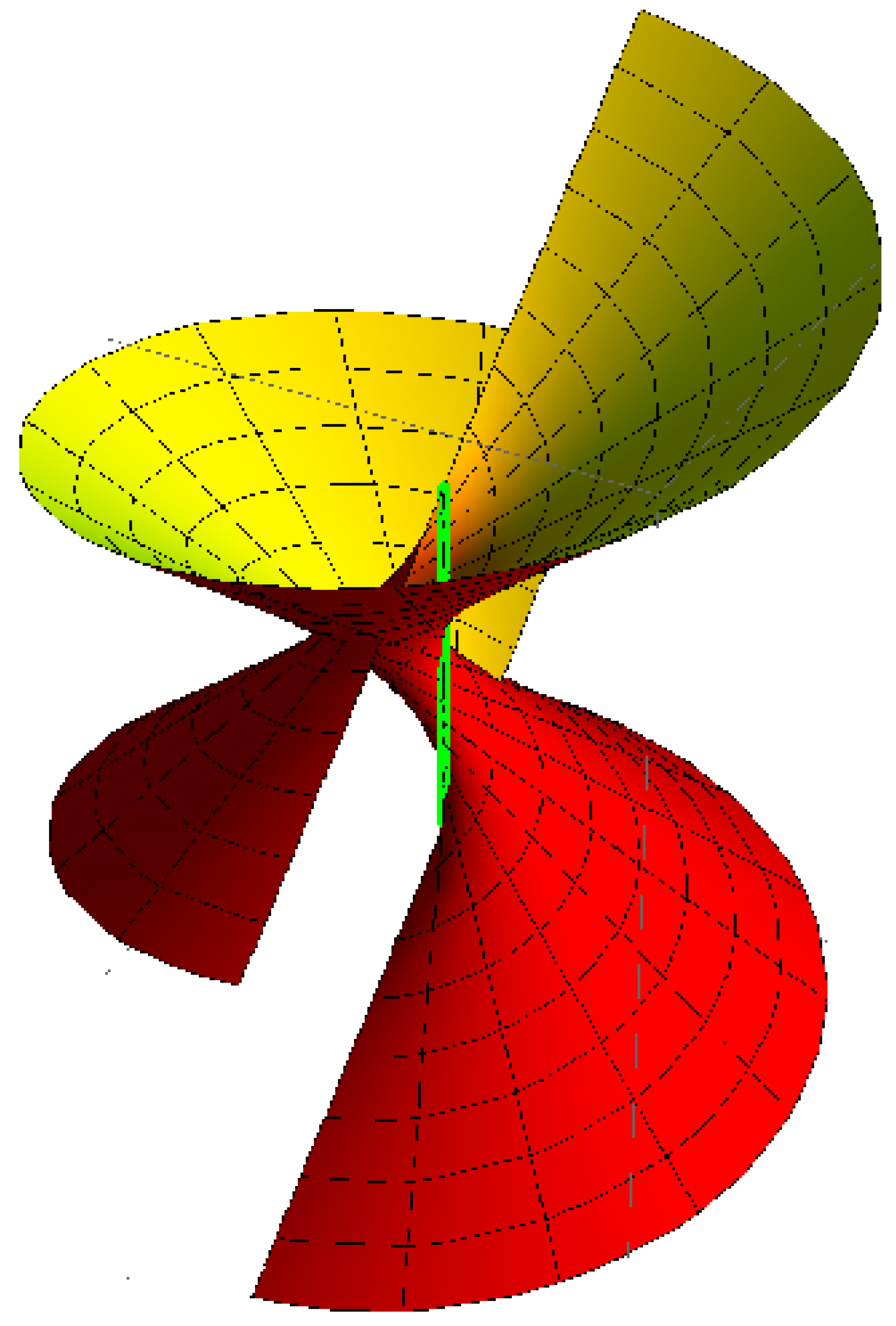
Timelike Archimedes with its striction curve is a timelike line: for $\beta =1$, ${\varphi }^{*}=0$, $\varphi =1.3$, $-3\le v\le 3$, and $-\pi \le \phi \le \pi$ (see Figure 6).

(4)

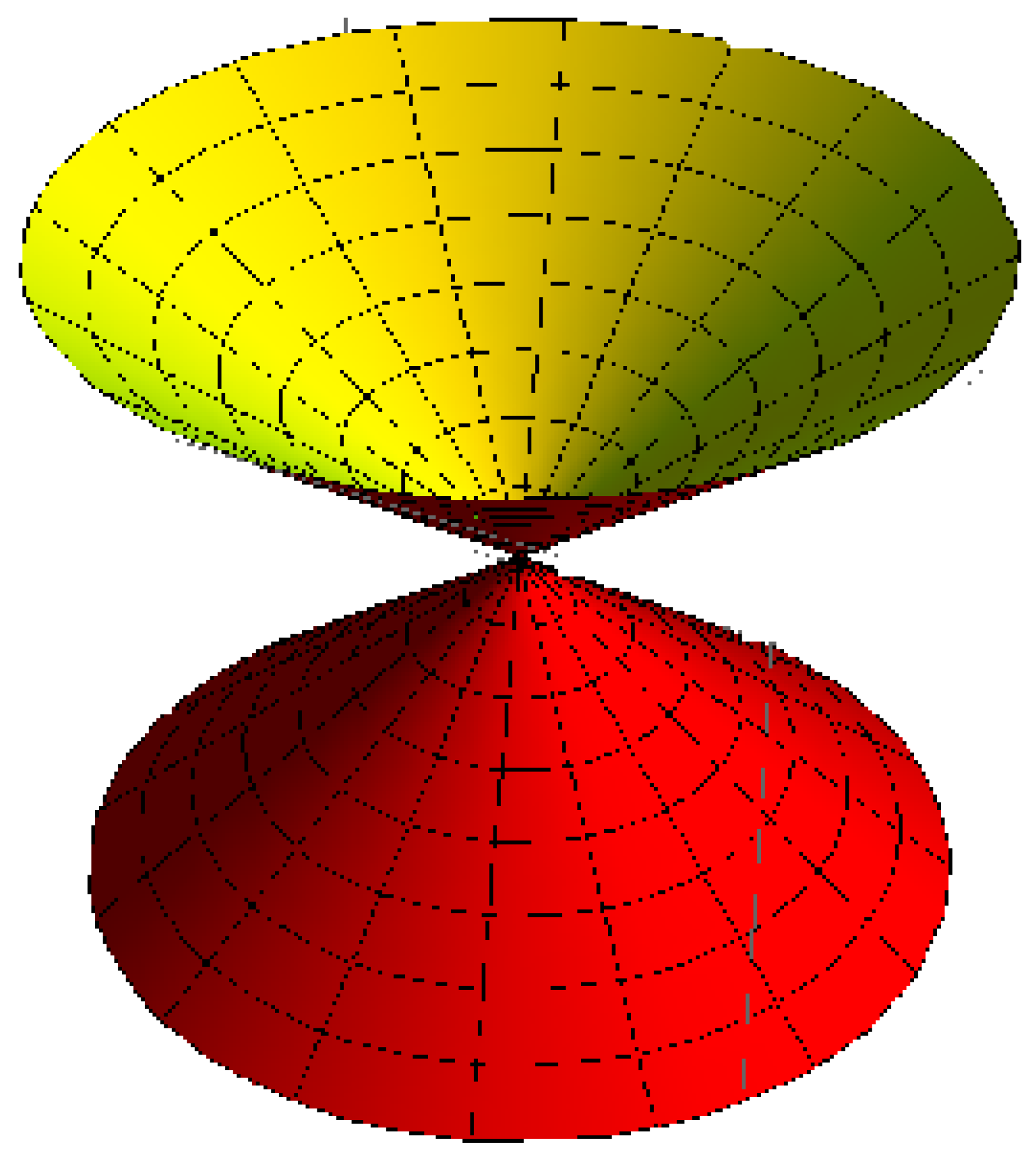
Timelike circular cone with its striction curve is a fixed point: for $\beta ={\varphi }^{*}=0$, $\varphi =0.5$, $-2.5\le v\le 2.5$, and $0\le \phi \le 2\pi$ (see Figure 7).

(5)

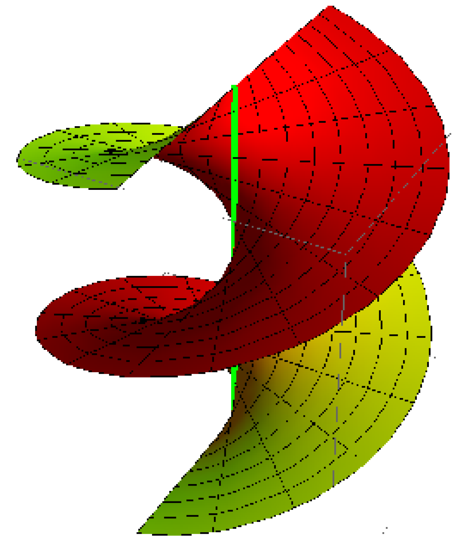
Timelike helicoid of the 1st kind with its striction curve is a timelike line: for $\beta =1$, ${\varphi }^{*}=\varphi =0$, $-3\le v\le 3$, and $-\pi \le \phi \le \pi$ (see Figure 8).

4. Conclusions

This work supplies the kinematic geometry for a timelike ruled surface with stationary timelike Disteli-axis by the similarity with Lorentzian dual spherical kinematics. This supplies the ability to derive set of invariants which discover the local shape of timelike ruled surface. Hence, the Lorentzian form of the well-known equation of the Plücker’s conoid has been concluded and its kinematic-geometry are explained in detail. Finally, a description for a timelike line trajectory to be a stationary timelike Disteli-axis is extracted and examined. These results have the potential to expand the use of geometric properties of timelike ruled surfaces created by spacelike lines embedded in spatial mechanisms. Our results in this paper can contribute to the field of spatial kinematics and have practical implementations in mechanical mathematics and engineering. In future work, we plan to proceed to research some implementations of timelike ruled surfaces as tooth flanks for gears with skew timelike axes such that at any instant the contact points are located on a timelike line as in [17,18,19].

References

- Bottema, O.; Roth, B. Theoretical Kinematics; North-Holland Press: New York, NY, USA, 1979. [Google Scholar]
- Karger, A.; Novak, J. Space Kinematics and Lie Groups; Gordon and Breach Science Publishers: New York, NY, USA, 1985. [Google Scholar]
- Pottman, H.; Wallner, J. Computational Line Geometry; Springer: Berlin/Heidelberg, Germany, 2001. [Google Scholar]
- Köse, Ö.C.C.; Sarıoglu, B.K.; Karakılıç, I. Kinematic differential geometry of a rigid body in spatial motion using dual vector calculus: Part II. Appl. Math. 2006, 182, 333–358. [Google Scholar] [CrossRef]
- Abdel-Baky, R.A.; Al-Ghefari, R.A. On the one-parameter dual spherical motions. Comp. Aided Geom. Design 2011, 28, 23–37. [Google Scholar] [CrossRef]
- Turhan, T.; Ayyıldız, N. A Study on Geometry of Spatial Kinematics in Lorentzian Space; Süleyman Demirel Üniversitesi Fen Bilimleri Enstitüsü Dergisi: Isparta, Türkiye, 2017; Volume 21, pp. 808–811. [Google Scholar]
- Gilani, S.M.; Abazari, N.; Yayli, Y. Characterizations of dual curves and dual focal curves in dual Lorentzian space . Turk J. Math 2020, 44, 1561–1577. [Google Scholar] [CrossRef]
- Aslan, M.C.; Sekerci, G.A. Dual curves associated with the Bonnet ruled surfaces. Int. J. Geom. Methods Mod. Phys. 2020, 17, 2050204. [Google Scholar] [CrossRef]
- Abdel-Baky, R.A.; Unluturk, Y. A new construction of timelike ruled surfaces with stationarfy Disteli-axis. Honam Math. J. 2020, 42, 551–568. [Google Scholar]
- Makki, R. Some characterizations of non-null rectifying curves in dual Lorentzian 3-space . AIMS Math. 2021, 6, 2114–2131. [Google Scholar] [CrossRef]
- Alluhaibi, N.S.; Abdel-Baky, R.A. Kinematic geometry of timelike ruled surfaces in Minkowski 3-space . Symmetry 2022, 14, 749. [Google Scholar] [CrossRef]
- Mofarreh, F. Timelike ruled and developable surfaces in Minkowski 3-space . Front. Phys. 2022, 10, 148. [Google Scholar] [CrossRef]
- O’Neil, B. Semi-Riemannian Geometry Geometry, with Applications to Relativity; Academic Press: New York, NY, USA, 1983. [Google Scholar]
- Walfare, J. Curves and Surfaces in Minkowski Space. Ph.D. Thesis, Faculty of Science, Leuven, Belgium, 1995. [Google Scholar]
- Bruce, J.W.; Giblin, P.J. Curves and Singularities, 2nd ed.; Cambridge University Press: Cambridge, UK, 1992. [Google Scholar]
- Cipolla, R.; Giblin, P.J. Visual Motion of Curves and Surfaces; Cambridge University Press: Cambridge, UK, 2000. [Google Scholar]
- Alluhaibi, N.A.; Abdel-Baky, R.A. On the kinematic-geometry of one-parameter Lorentzian spatial movement. Int. J. Adv. Manuf. Technol. 2022, 121, 7721–7731. [Google Scholar] [CrossRef]
- Stachel, H. On spatial involute gearing. In Proceedings of the 6th International Conference on Applied Informatics (ICAI), Eger, Hungary, 27–31 January 2004. [Google Scholar]
- Figlioini, G.; Stachel, H.; Angeles, J. The computational fundamentals of spatial cycloidal gearing. In Computational Kinematics: Proceedings of the 5th International Workshop on Computational Kinematics; Kecskemethy, A., Muller, A., Eds.; Springer: Berlin/Heidelberg, Germany, 2009; pp. 375–384. [Google Scholar]
Figure 1.
The dual hyperbolic and dual Lorentzian unit spheres.
Figure 4.
General timelike helicoidal surface.
Figure 5.
Lorentzian sphere.
Figure 6.
Timelike Archimedes.
Figure 7.
Timelike cone.
Figure 8.
A timelike helicoid of the 1st kind.
Disclaimer/Publisher’s Note: The statements, opinions and data contained in all publications are solely those of the individual author(s) and contributor(s) and not of MDPI and/or the editor(s). MDPI and/or the editor(s) disclaim responsibility for any injury to people or property resulting from any ideas, methods, instructions or products referred to in the content. |
© 2023 by the authors. Licensee MDPI, Basel, Switzerland. This article is an open access article distributed under the terms and conditions of the Creative Commons Attribution (CC BY) license (https://creativecommons.org/licenses/by/4.0/).
Share and Cite
MDPI and ACS Style
Almoneef, A.A.; Abdel-Baky, R.A. Timelike Ruled Surfaces with Stationary Disteli-Axis. Symmetry 2023, 15, 998. https://doi.org/10.3390/sym15050998
AMA Style
Almoneef AA, Abdel-Baky RA. Timelike Ruled Surfaces with Stationary Disteli-Axis. Symmetry. 2023; 15(5):998. https://doi.org/10.3390/sym15050998
Chicago/Turabian StyleAlmoneef, Areej A., and Rashad A. Abdel-Baky. 2023. "Timelike Ruled Surfaces with Stationary Disteli-Axis" Symmetry 15, no. 5: 998. https://doi.org/10.3390/sym15050998
Note that from the first issue of 2016, this journal uses article numbers instead of page numbers. See further details here.