Extension of King’s Iterative Scheme by Means of Memory for Nonlinear Equations

Abstract

We developed a new family of optimal eighth-order derivative-free iterative methods for finding simple roots of nonlinear equations based on King’s scheme and Lagrange interpolation. By incorporating four self-accelerating parameters and a weight function in a single variable, we extend the proposed family to an efficient iterative scheme with memory. Without performing additional functional evaluations, the order of convergence is boosted from 8 to $15.51560$, and the efficiency index is raised from $1.6817$ to $1.9847$. To compare the performance of the proposed and existing schemes, some real-world problems are selected, such as the eigenvalue problem, continuous stirred-tank reactor problem, and energy distribution for Planck’s radiation. The stability and regions of convergence of the proposed iterative schemes are investigated through graphical tools, such as 2D symmetric basins of attractions for the case of memory-based schemes and 3D stereographic projections in the case of schemes without memory. The stability analysis demonstrates that our newly developed schemes have wider symmetric regions of convergence than the existing schemes in their respective domains.

1. Introduction

Solving nonlinear equations or root finding is an essential task in numerical analysis and has a wide range of applications in physics, chemistry, mathematical biology, medicines, economics, and engineering. Numerical or iterative methods to find approximate solutions of nonlinear equations are the most frequently used techniques. One can distinguish between two common approaches for numerical solutions of nonlinear equations, namely one-point and multipoint iterative schemes. Newton’s method is one of the famous root-finding methods for solving a single nonlinear equation $f\left(x\right)=0$, given as follows [1]:

$$x_m=x_m-\frac{f\left(x_m\right)}{f^{\prime }\left(x_m\right)},m\ge 0,$$

(1)

where f is a real valued function. Newton’s scheme is a one-point method and is quadratically convergent in some neighborhood of the root $\eta$ of f for an initial guess $x_0$ close enough to $\eta$. There are several two-point methods to find simple roots of $f\left(x\right)=0$ in the literature. Among them, King’s method is the most popular two-point fourth-order method [2], which is given as follows:

$$\begin{array}{ccc}\hfill y_m& =& x_m-\frac{f\left(x_m\right)}{f^{\prime }\left(x_m\right)},m\ge 0,\hfill \\ \hfill z_m& =& y_m-\frac{f\left(x_m\right)+\gamma f\left(y_m\right)}{f\left(x_m\right)+(\gamma -2)f\left(y_m\right)}\frac{f\left(y_m\right)}{f^{\prime }\left(x_m\right)},\gamma \in \mathbb{R}.\hfill \end{array}$$

(2)

Multipoint iterative schemes gained much interest at the beginning of the twenty-first century, since they overcome the theoretical limits of one-point methods regarding convergence speed and computational efficiency. Some root-finding schemes based on multipoint iterations are first studied in the books by Traub [1] and Ostrowski [3] and the papers in [2,4], published in the twentieth century. Multipoint schemes can be further classified into two categories: “methods with memory” and “methods without memory”. A multipoint method using current information only is called a method without memory, while a method employing the current as well as previous information is known as a method with memory. An important aspect of the optimality of the methods with memory is that they improve the convergence order and efficiency index of the iterative schemes without memory without using additional function evaluations. Moreover, this approach makes it an impactful class of multipoint iterative methods. Kung and Traub conjectured that an iterative scheme without memory based on r evaluations of function could obtain an order of convergence of at most $2^{r-1}$ (known as optimal order). The computational efficiency index of an iterative method is expressed as $2^{\frac{r-1}{r}}$ [3].

Traub [1] proposed a uniparametric derivative-free scheme with memory by a slight modification of Steffensen’s iterative method [5] for suitably chosen $x_0,{\phi }_0$ as follows:

$$\begin{array}{ccc}\hfill {\nu }_m& =& x_m+{\phi }_{m}f\left(x_m\right),m\ge 0,\hfill \\ \hfill x_m& =& x_m-\frac{f\left(x_m\right)}{f\left[{\nu }_m,x_m\right]},{\phi }_m=-\frac{1}{N_1^{\prime }\left(x_m\right)},\hfill \end{array}$$

(3)

where $f[v,x]=\frac{f\left(v\right)-f\left(x\right)}{(v-x)}$ denotes divided difference of first order, $N_1=f\left(x_m\right)+\left(x-x_m\right)f\left[{\nu }_m,x_m\right]$, and ${\phi }_m$ is the free accelerating parameter. The iterative scheme with memory (3) has a convergence order of $2.41$. Several researchers have developed root-finding methods using memory based on existing optimal methods without memory; see, e.g., [2,6,7,8,9,10,11,12,13,14,15,16].

It is a common fact that iterative schemes are very sensitive towards an initial guess. To resolve this difficulty, we identify the region in which a root lies and, as a result, a variety of safe initial guesses are available to choose from. The convergence regions and stability of an iterative scheme can be visualized in 2D dynamical planes with the help of symmetric basins of attractions and drawing the 3D stereographic projections on the sphere.

One of the biggest challenges of iterative processes is to verify that they converge to the exact solution, rather than getting stuck in a local minimum or diverging. An effective way for examining the behavior of iterative methods, particularly those based on fixed-point iterations, is the analysis of basins of attractions. The areas of the parameter space that correspond to the same solution are referred to as basins of attractions. The conditions under which the iterative approach converges, as well as the rate of convergence and the stability of the solution, can be found by examining the basins of attractions. This information is essential for choosing the best iterative approach for a particular problem, as well as for adjusting a method’s parameters to determine how well it performs.

Motivated and inspired by the research being conducted in this direction, we developed a new modified King’s type scheme with memory, having a convergence order of at least $15.5156$ based on Lagrange interpolation. In Section 2, we present a new optimal eighth-order derivative-free iterative family without memory. In Section 3, we extend the proposed optimal scheme without memory presented in Section 2 to an iterative scheme with memory and provide its convergence analysis. In Section 4, we present some particular cases of the weight functions and iterative methods corresponding to the weight functions. In Section 5, we give applications of the presented iterative methods to solve engineering problems, such as the energy distribution for Planck’s radiation and continuous stirred-tank reactor. A comparison of the newly developed iterative scheme with already existing similar schemes is also presented in Section 5 by using different test functions. In Section 6, we present the extensive stability analysis of the proposed scheme without memory by drawing its 3D stereographic projections. In Section 7, we present dynamical analysis of the proposed iterative scheme with memory with the help of its 2D symmetric basins of attractions. Finally, the conclusions are discussed in Section 8.

2. Extension of King’s Method to an Optimal Eighth-Order Derivative-Free Scheme

Our primary aim is to develop an optimal eighth-order method without memory based on Lagrange interpolation which can be extended to an iterative scheme with memory. By adding Newton’s method to the third step of King’s method (2), we obtain

$$\begin{array}{ccc}\hfill q_m& =& x_m-\frac{f\left(x_m\right)}{f^{\prime }\left(x_m\right)},\hfill \\ \hfill h_m& =& q_m-\frac{f\left(q_m\right)}{f^{\prime }\left(x_m\right)}\frac{f\left(x_m\right)+\omega f\left(q_m\right)}{f\left(x_m\right)+(\omega -2)f\left(q_m\right)},\hfill \\ \hfill x_{m+1}& =& h_m-\frac{f\left(h_m\right)}{f^{\prime }\left(h_m\right)}.\hfill \end{array}$$

(4)

The three-step iterative scheme (4) is not optimal because it needs five evaluations of functions to provide eighth-order convergence. To make it optimal, derivative-free, and extendable to a with-memory scheme, we adopt the following procedure.

We use the approximation of the derivative $f^{\prime }\left(x_m\right)$ in the first step of the iterative method (4) as follows:

$$f^{\prime }\left(x_m\right)\approx f[{\nu }_m,x_m]+{\beta }_{2}f\left({\nu }_m\right),$$

(5)

where ${\nu }_m=x_m+{\beta }_{1}f\left(x_m\right)$.

The derivative $f^{\prime }\left(x_m\right)$ in the second step is replaced by the following approximation (with a weight function $U,$ depending on variable $s_m=\frac{f\left(q_m\right)}{f\left(x_m\right)}$):

$$f^{\prime }\left(x_m\right)\approx \frac{f[q_m,{\nu }_m]+{\beta }_{2}f\left({\nu }_m\right)+{\beta }_3(q_m-{\nu }_m)(q_m-x_m)}{{}^{U\left(s_m\right)}}.$$

(6)

We replace the derivative $f^{\prime }\left(h_m\right)$ in the third step of the iterative scheme (4) by the following approximation:

$$f^{\prime }\left(h_m\right)\approx L_3^{\prime }\left(h_m\right)+{\beta }_4(h_m-{\nu }_m)(h_m-q_m)(h_m-x_m),$$

(7)

where ${\beta }_1,{\beta }_2,{\beta }_3,$ and ${\beta }_4$ are free parameters and

$$\begin{array}{ccc}\hfill L_3^{\prime }\left(h_m\right)& =& f[h_m,{\nu }_m]+f[h_m,x_m]+f[h_m,q_m]-f[x_m,q_m]-f[{\nu }_m,q_m]-f[x_m,{\nu }_m]\hfill \\ & & +\frac{(x_m-h_m)f\left(x_m\right)}{(x_m-{\nu }_m)(x_m-q_m)}+\frac{({\nu }_m-h_m)f\left({\nu }_m\right)}{({\nu }_m-x_m)({\nu }_m-q_m)}+\frac{(q_m-h_m)f\left(q_m\right)}{(q_m-{\nu }_m)(q_m-x_m)},\hfill \end{array}$$

where $L_3^{\prime }\left(h_m\right)$ is the derivative of Lagrange interpolating polynomial of degree three that interpolates $x_m,{\nu }_m,q_m,$ and $h_m$.

By using the above approximations, we obtain the following eighth-order iterative method without memory using four function evaluations per cycle:

$$\begin{array}{ccc}\hfill {\nu }_m& =& x_m+{\beta }_{1}f\left(x_m\right),\hfill \\ \hfill q_m& =& x_m-\frac{f\left(x_m\right)}{f[{\nu }_m,x_m]+{\beta }_{2}f\left({\nu }_m\right)},\hfill \\ \hfill h_m& =& q_m-U\left(s_m\right)\left(\frac{f\left(q_m\right)}{f[q_m,{\nu }_m]+{\beta }_{2}f\left({\nu }_m\right)+{\beta }_3(q_m-{\nu }_m)(q_m-x_m)}\right)\hfill \\ & & \left(\frac{f\left(x_m\right)+\omega f\left(q_m\right)}{f\left(x_m\right)+(\omega -2)f\left(q_m\right)}\right),\hfill \\ \hfill x_m& =& h_m-\frac{f\left(h_m\right)}{R_m},\hfill \end{array}$$

(8)

where

$$\begin{array}{ccc}\hfill R_m& =& f[h_m,{\nu }_m]+f[h_m,x_m]+f[h_m,q_m]-f[x_m,q_m]-f[{\nu }_m,q_m]-f[x_m,{\nu }_m]\hfill \\ & & +\frac{(x_m-h_m)f\left(x_m\right)}{(x_m-{\nu }_m)(x_m-q_m)}+\frac{({\nu }_m-h_m)f\left({\nu }_m\right)}{({\nu }_m-x_m)({\nu }_m-q_m)}+\frac{(q_m-h_m)f\left(q_m\right)}{(q_m-{\nu }_m)(q_m-x_m)}\hfill \\ & & +{\beta }_4(h_m-{\nu }_m)(h_m-q_m)(h_m-x_m).\hfill \end{array}$$

The next theorem indicates that the proposed method without memory (8) has a convergence order of eight with an efficiency index of $8^{\frac{1}{4}}\approx 1.68179$.

Theorem 1.

Suppose that $f:I_f\subset \mathbb{R}\to \mathbb{R}$ is sufficiently differentiable and $\eta \in I_f$ is a real root of an equation $f\left(x\right)=0$, where $I_f\subset \mathbb{R}$ is an open interval and $x_0$ is a good initial guess close to root η. Then, the convergence order of four parametric three-step schemes (8) is at least eight if the following conditions hold for the weight function $U\left(s_m\right)$:

$$U\left(0\right)=1,U^{\prime }\left(0\right)=-1,U^{″}\left(0\right)=2,$$

(9)

and the error equation of the iterative scheme (8) for all values of ${\beta }_1,{\beta }_2,{\beta }_3$, and ${\beta }_4$ is given as

$$\begin{array}{ccc}\hfill e_{m+1}& =& \frac{1}{f^{\prime }{\left(\eta \right)}^2}({(C_2+{\beta }_2)}^2{({\beta }_1{f}^{\prime }\left(\eta \right)+1)}^4(2f^{\prime }{\left(\eta \right)}^2\omega c_2^2{\beta }_1+4f^{\prime }{\left(\eta \right)}^2{C}_2{\beta }_1{\beta }_2\omega \hfill \\ & & +2f^{\prime }{\left(\eta \right)}^2{\beta }_1{\beta }_2^2\omega -2f^{\prime }{\left(\eta \right)}^2{C}_2^2{\beta }_1-4{\beta }_2{f}^{\prime }{\left(\eta \right)}^2{\beta }_1{C}_2-2f^{\prime }{\left(\eta \right)}^2{\beta }_1{\beta }_2^2+2f^{\prime }\left(\eta \right)C_2^2\omega \hfill \\ & & +4f^{\prime }\left(\eta \right)C_2{\beta }_2\omega +2f^{\prime }{\left(\eta \right)}^2{\beta }_2^2\omega -2{\beta }_2{f}^{\prime }\left(\eta \right)C_2-2f^{\prime }\left(\eta \right){\beta }_2^2-f^{\prime }\left(\eta \right)C_3+{\beta }_3)\hfill \\ & & (2f^{\prime }{\left(\eta \right)}^2\omega c_2^3{\beta }_1+4f^{\prime }{\left(\eta \right)}^2\omega C_2^2{\beta }_1{\beta }_2+2f^{\prime }{\left(\eta \right)}^2\omega C_2{\beta }_1{\beta }_2^2-2f^{\prime }{\left(\eta \right)}^2{C}_2^3{\beta }_1\hfill \\ & & -4f^{\prime }{\left(\eta \right)}^2{\beta }_1{\beta }_2{C}_2^2-2f^{\prime }{\left(\eta \right)}^2{C}_2{\beta }_1{\beta }_2^2+2f^{\prime }\left(\eta \right)\omega C_2^3+4f^{\prime }\left(\eta \right)\omega C_2^2{\beta }_2+2f^{\prime }\left(\eta \right)\omega C_2{\beta }_2^2\hfill \\ & & -2f^{\prime }\left(\eta \right)C_2^2{\beta }_2-2f^{\prime }\left(\eta \right)C_2{\beta }_2^2-f^{\prime }\left(\eta \right)C_2{C}_3+f^{\prime }\left(\eta \right)C_4+C_2{\beta }_3\hfill \\ & & -{\beta }_4\left)\right)e_m^8+O\left(e_m^9\right).\hfill \end{array}$$

(10)

Proof. 

Let $e_m$ be the error in the root η at $m\mathrm{th}$ step, specified as

$$e_m=x_m-\eta .$$

Expanding $f\left(x_m\right)$ using Taylor series, we obtain

$$f\left(x_m\right)=f^{\prime }\left(\eta \right)(e_m+C_2{e}_m^2+C_3{e}_m^3+C_4{e}_m^4+C_5{e}_m^5+C_6{e}_m^6+C_7{e}_m^7+C_8{e}_m^8)+O\left(e_m^9\right),$$

where

$$C_n=\frac{f^{\left(n\right)}\left(\eta \right)}{n!f^{\prime }\left(\eta \right)},n\ge \eta .$$

We obtain the error term $e_{m,\xi }={\nu }_m-\eta$ by using Taylor’s expansion:

$$e_{m,\xi }=(1+{\beta }_1{f}^{\prime }\left(\eta \right))e_m+{\beta }_1{f}^{\prime }\left(\eta \right)(C_2{e}_m^2+C_3{e}_m^3+C_4{e}_m^4+C_5{e}_m^5+C_6{e}_m^6+C_7{e}_m^7+C_8{e}_m^8)+O\left(e_n^9\right).$$

Similarly, by applying Taylor’s series, we obtain $f\left({\eta }_m\right),$ which is given as follows:

$$f\left({\nu }_m\right)=f^{\prime }\left(\eta \right)((1+{\beta }_1{f}^{\prime }\left(\eta \right))e_m+{\beta }_1{f}^{\prime }\left(\eta \right)C_2{e}_m^2+\cdots +O\left(e_m^9\right)).$$

Thus, the error term of $q_m$ is

$$e_{m,w}=(C_2+{\beta }_2)(1+{\beta }_1{f}^{\prime }\left(\eta \right))e_m^2+\cdots +O\left(e_m^9\right),$$

where

$$e_{m,w}=q_m-\eta .$$

By applying Taylor’s expansion, we obtain $f\left(q_m\right)$, which is given as

$$f\left(q_m\right)=f^{\prime }\left(\eta \right)[(C_2+{\beta }_2)(1+{\beta }_1{f}^{\prime }\left(\eta \right))e_m^2+\cdots +O\left(e_m^9\right)].$$

Again, by Taylor’s series, we obtained the error expression of $h_m$ as follows:

$$\begin{array}{ccc}\hfill e_{m,z}& =& -(C_2+{\beta }_2)(U\left(0\right)-1)(f^{\prime }\left(\eta \right){\beta }_1+1)e_n^2+(3{\beta }_1{f}^{\prime }\left(\eta \right)C_3-U^{\prime }\left(0\right)f^{\prime }{\left(\eta \right)}^2{C}_2^2{\beta }_1\hfill \\ & & -U^{\prime }\left(0\right)f^{\prime }{\left(\eta \right)}^2{\beta }_1^2{\beta }_2^2-2U^{\prime }\left(0\right)f^{\prime }\left(\eta \right)C_2^2{\beta }_1-2U^{\prime }\left(0\right)f^{\prime }\left(\eta \right){\beta }_1{\beta }_2^2-U\left(0\right)f^{\prime }{\left(\eta \right)}^2{C}_2{\beta }_1^2{\beta }_2\hfill \\ & & -2U\left(0\right)f^{\prime }\left(\eta \right)C_2{\beta }_1{\beta }_2-2f^{\prime }\left(\eta \right){\beta }_1{\beta }_2^2{f}^{\prime }{\left(\eta \right)}^2{\beta }_1^2{\beta }_2^2-U^{\prime }\left(0\right)C_2^2-U^{\prime }\left(0\right){\beta }_2^2\hfill \\ & & -2U^{\prime }\left(0\right)f^{\prime }{\left(\eta \right)}^2{C}_2{\beta }_1^2{\beta }_2-4U^{\prime }\left(0\right)f^{\prime }\left(\eta \right)C_2{\beta }_1{\beta }_2-2{\beta }_2{C}_2-f^{\prime }{\left(\eta \right)}^2{C}_2{\beta }_1^2{\beta }_2\hfill \\ & & -2{\beta }_2{f}^{\prime }\left(\eta \right){\beta }_1{C}_2-2C_2^2+f^{\prime }{\left(\eta \right)}^2{C}_3{\beta }_1^2-2{\beta }_1{f}^{\prime }\left(\eta \right)C_2^2-{\beta }_1^2{f}^{\prime }{\left(\eta \right)}^2{C}_2^2+U\left(0\right)C_2^2\hfill \\ & & -2U\left(0\right)C_3-2U^{\prime }\left(0\right)C_2{\beta }_2-U\left(0\right)f^{\prime }{\left(\eta \right)}^{2}C{c}_3{\beta }_1^2-3U\left(0\right)f^{\prime }\left(\eta \right)C_3{\beta }_1+2C_3\hfill \\ & & -{\beta }_2^2)e_m^3+\cdots +O\left(e_m^9\right).\hfill \end{array}$$

(11)

In order to achieve fourth-order convergence, we choose $U\left(0\right)=1,U^{\prime }\left(0\right)=-1,$ and $U^{″}\left(0\right)=2$; we have an error term of $h_m$:

$$\begin{array}{ccc}\hfill e_{m,z}& =& \frac{1}{f^{\prime }\left(\eta \right)}\left({(f^{\prime }\left(\eta \right){\beta }_1+1)}^2(C_2+{\beta }_2)\right(2f^{\prime }{\left(\eta \right)}^2\omega c_2^2{\beta }_1+4f^{\prime }{\left(\eta \right)}^2{C}_2{\beta }_1{\beta }_2\omega +2f^{\prime }{\left(\eta \right)}^2{\beta }_1{\beta }_2^2\omega \hfill \\ & & -2f^{\prime }{\left(\eta \right)}^2{C}_2^2{\beta }_1-4{\beta }_2{f}^{\prime }{\left(\eta \right)}^2{\beta }_1{C}_2-2f^{\prime }{\left(\eta \right)}^2{\beta }_1{\beta }_2^2+2f^{\prime }\left(\eta \right)C_2^2\omega +4f^{\prime }\left(\eta \right)C_2{\beta }_2\omega \hfill \\ & & +2f^{\prime }{\left(\eta \right)}^2{\beta }_2^2\omega -2{\beta }_2{f}^{\prime }\left(\eta \right)C_2-2f^{\prime }\left(\eta \right){\beta }_2^2-f^{\prime }\left(\eta \right)C_3+{\beta }_3)e_m^4+\cdots +O\left(e_m^9\right).\hfill \end{array}$$

By using the Taylor’s series, we can easily find the expression of $f\left(h_m\right)$ and $R_m$ that is given in the newly proposed with-memory method (8). Thus, we obtain a convergence order of eight in the proposed iterative scheme (8) as follows:

$$\begin{array}{ccc}\hfill e_{m+1}& =& \frac{1}{f^{\prime }{\left(\eta \right)}^2}({(C_2+{\beta }_2)}^2{({\beta }_1{f}^{\prime }\left(\eta \right)+1)}^4(2f^{\prime }{\left(\eta \right)}^2\omega c_2^2{\beta }_1+4f^{\prime }{\left(\eta \right)}^2{C}_2{\beta }_1{\beta }_2\omega \hfill \\ & & +2f^{\prime }{\left(\eta \right)}^2{\beta }_1{\beta }_2^2\omega -2f^{\prime }{\left(\eta \right)}^2{C}_2^2{\beta }_1-4{\beta }_2{f}^{\prime }{\left(\eta \right)}^2{\beta }_1{C}_2-2f^{\prime }{\left(\eta \right)}^2{\beta }_1{\beta }_2^2+2f^{\prime }\left(\eta \right)C_2^2\omega \hfill \\ & & +4f^{\prime }\left(\eta \right)C_2{\beta }_2\omega +2f^{\prime }{\left(\eta \right)}^2{\beta }_2^2\omega -2{\beta }_2{f}^{\prime }\left(\eta \right)C_2-2f^{\prime }\left(\eta \right){\beta }_2^2-f^{\prime }\left(\eta \right)C_3+{\beta }_3)\hfill \\ & & (2f^{\prime }{\left(\eta \right)}^2\omega C_2^3{\beta }_1+4f^{\prime }{\left(\eta \right)}^2\omega C_2^2{\beta }_1{\beta }_2+2f^{\prime }{\left(\eta \right)}^2\omega C_2{\beta }_1{\beta }_2^2-2f^{\prime }{\left(\eta \right)}^2{C}_2^3{\beta }_1\hfill \\ & & -4f^{\prime }{\left(\eta \right)}^2{\beta }_1{\beta }_2{C}_2^2-2f^{\prime }{\left(\eta \right)}^2{C}_2{\beta }_1{\beta }_2^2+2f^{\prime }\left(\eta \right)\omega C_2^3+4f^{\prime }\left(\eta \right)\omega C_2^2{\beta }_2+2f^{\prime }\left(\eta \right)\omega C_2{\beta }_2^2\hfill \\ & & -2f^{\prime }\left(\eta \right)C_2^2{\beta }_2-2f^{\prime }\left(\eta \right)C_2{\beta }_2^2-f^{\prime }\left(\eta \right)C_2{C}_3+f^{\prime }\left(\eta \right)C_4+C_2{\beta }_3\hfill \\ & & -{\beta }_4\left)\right)e_m^8+O\left(e_n^9\right).\hfill \end{array}$$

(12)

□

Remark 1.

The above theorem verifies that the proposed method (8) has eighth-order convergence with an efficiency index of $8^{\frac{1}{4}}\approx 1.68179.$ Furthermore, note that if we chose ${\beta }_1=-\frac{1}{f^{\prime }\left(\eta \right)}$ and ${\beta }_2=-C_2$, then the coefficient of $e_m^8$ vanishes and we obtain the following error equation:

$$e_{m+1}=\left[C_2^4{C}_3^3\left({\beta }_3-f^{\prime }\left(\eta \right)C_3\right)\left(C_2\left({\beta }_3-f^{\prime }\left(\eta \right)C_3\right)+f^{\prime }\left(\eta \right)C_4-{\beta }_4\right)\right]\frac{e_m^{14}}{f^{{}^{″}}\left(\eta \right)}+O\left(e_m^{15}\right).$$

By choosing ${\beta }_3=f^{\prime }\left(\eta \right)C_3$ and ${\beta }_4=f^{\prime }\left(\eta \right)C_4,$ the resulting scheme has an optimal order of convergence of at least sixteen. In order to accomplish the with-memory iterative scheme, parameters play an essential role. Thus, from the above error analysis, we observe that the multipoint scheme (8) is extendable to an iterative scheme with memory.

3. Efficient King’s Type Scheme with Memory

This section covers a significant role in our work. Here, we extend the proposed optimal scheme (8) such that it achieves the highest possible order and efficiency by using previous iteration values. We use four self-accelerating parameters, ${\beta }_1,{\beta }_2,{\beta }_3,$ and ${\beta }_4$ in the scheme (8) and approximate these parameters by Newton’s interpolatory polynomial of the appropriate degree. So, in this way, we can increase the order of convergence. If we choose ${\beta }_1=-\frac{1}{f^{\prime }\left(\eta \right)},{\beta }_2=-C_2,$${\beta }_3=f^{\prime }\left(\eta \right)C_3$ and ${\beta }_4=$ $f^{\prime }\left(\eta \right)C_4,$ where $C_j=\frac{f^{\left(j\right)}\left(\eta \right)}{j!f^{\prime }\left(\eta \right)}$ and $j\ge 2$, then the order of convergence reaches up to sixteen. Thus, to obtain an iterative scheme with memory, the parameters ${\beta }_1,{\beta }_2,{\beta }_3,$ and ${\beta }_4$ are determined by using the following formulas:

$${\beta }_1={\beta }_{1,m}=-\frac{1}{N_4^{{}^{\prime }}\left(x_m\right)}\approx -\frac{1}{f^{\prime }\left(\eta \right)},$$

$${\beta }_2={\beta }_{2,m}=-\frac{N_5^{″}\left({\nu }_m\right)}{2N_5^{{}^{\prime }}\left({\nu }_m\right)}\approx -C_2,$$

$${\beta }_3={\beta }_{3,m}=-\frac{N_6^{{}^{‴}}\left(q_m\right)}{6}\approx f^{\prime }\left(\eta \right)C_3,$$

$${\beta }_4={\beta }_{4,m}=-\frac{N_7^{{}^{iv}}\left(h_m\right)}{24}\approx f^{\prime }\left(\eta \right)C_4.$$

(13)

The above approximations are made by using Newton’s fourth-, fifth-, sixth-, and seventh-degree interpolatory polynomials, passing through the best available approximations, and they are given as follows:

$$\begin{array}{ccc}\hfill N_4\left(\phi \right)& =& N_4\left(\phi ;x_m,h_m,q_m,{\nu }_m,x_m\right),\hfill \\ \hfill N_5\left(\phi \right)& =& N_5\left(\phi ;{\nu }_m,x_m,h_m,q_m,{\nu }_m,x_m\right),\hfill \\ \hfill N_6\left(\phi \right)& =& N_6\left(\phi ;q_m,{\nu }_m,x_m,h_m,q_m,{\nu }_m,x_m\right),\hfill \\ \hfill N_7\left(\phi \right)& =& N_7\left(\phi ;h_m,q_m,{\nu }_m,x_m,h_m,q_m,{\nu }_m,x_m\right),\hfill \end{array}$$

for any $m\ge 1$. The explicit representations for $N_4\left(\phi \right),N_5\left(\phi \right),N_6\left(\phi \right),$ and $N_7\left(\phi \right)$ are given as follows:

$$\begin{array}{ccc}& & N_4\left(\phi ;x_m,h_m,q_m,{\nu }_m,x_m\right)\hfill \\ & =& f\left(x_m\right)+f\left[x_m,h_m\right]\left(\phi -x_m\right)+f\left[x_m,h_m,q_m\right]\left(\phi -x_m\right)\left(\phi -h_m\right)\hfill \\ & & +f\left[x_m,h_m,q_m,{\nu }_m\right]\left(\phi -x_m\right)\left(\phi -h_m\right)\left(\phi -q_m\right)\hfill \\ & & +f\left[x_m,h_m,q_m,{\nu }_m,x_m\right]\left(\phi -x_m\right)\left(\phi -h_m\right)\left(\phi -q_m\right)\hfill \\ & & \left(\phi -{\nu }_m\right),\hfill \end{array}$$

(14)

$$\begin{array}{ccc}& & N_5\left(\phi ;{\nu }_m,x_m,h_m,q_m,{\nu }_m,x_m\right)\hfill \\ & =& f\left({\nu }_m\right)+f\left[{\nu }_m,x_m\right]\left(\phi -{\nu }_m\right)+f\left[{\nu }_m,x_m,h_m\right]\left(\phi -{\nu }_m\right)\left(\phi -x_m\right)\hfill \\ & & +f\left[{\nu }_m,x_m,h_m,q_m\right]\left(\phi -{\nu }_m\right)\left(\phi -x_m\right)\left(\phi -h_m\right)+f\left[{\nu }_m,x_m,h_m,q_m,{\nu }_m\right]\hfill \\ & & \left(\phi -{\nu }_m\right)\left(\phi -x_m\right)\left(\phi -h_m\right)\left(\phi -q_m\right)+f\left[{\nu }_m,x_m,h_m,q_m,{\nu }_m,x_m\right]\hfill \\ & & \left(\phi -{\nu }_m\right)\left(\phi -x_m\right)\left(\phi -h_m\right)\left(\phi -q_m\right)\left(\phi -{\nu }_m\right),\hfill \end{array}$$

(15)

$$\begin{array}{ccc}& & N_6\left(\phi ;q_m,{\nu }_m,x_m,h_m,q_m,{\nu }_m,x_m\right)\hfill \\ & =& f\left(q_m\right)+f\left[q_m,{\nu }_m\right]\left(\phi -q_m\right)+f\left[q_m,{\nu }_m,x_m\right]\left(\phi -q_m\right)\left(\phi -{\nu }_m\right)\hfill \\ & & +f\left[q_m,{\nu }_m,x_m,h_m\right]\left(\phi -q_m\right)\left(\phi -{\nu }_m\right)\left(\phi -x_m\right)+f\left[q_m,{\nu }_m,x_m,h_m,q_m\right]\hfill \\ & & \left(\phi -q_m\right)\left(\phi -{\nu }_m\right)\left(\phi -x_m\right)\left(\phi -h_m\right)+f\left[q_m,{\nu }_m,x_m,h_m,q_m,{\nu }_m\right]\hfill \\ & & \left(\phi -q_m\right)\left(\phi -{\nu }_m\right)\left(\phi -x_m\right)\left(\phi -h_m\right)\left(\phi -q_m\right)\hfill \\ & & +f\left[q_m,{\nu }_m,x_m,h_m,q_m,{\nu }_m,x_m\right]\left(\phi -q_m\right)\left(\phi -{\nu }_m\right)\left(\phi -x_m\right)\hfill \\ & & \left(\phi -h_m\right)\left(\phi -q_m\right)\left(\phi -{\nu }_m\right),\hfill \end{array}$$

(16)

$$\begin{array}{ccc}& & N_7\left(\phi ;h_m,q_m,{\nu }_m,x_m,h_m,q_m,{\nu }_m,x_m\right)\hfill \\ & =& f\left(h_m\right)+f\left[h_m,q_m\right]\left(\phi -h_m\right)+f\left[h_m,q_m,{\eta }_x\right]\left(\phi -h_m\right)\left(\phi -q_m\right)\hfill \\ & & +f\left[h_m,q_m,{\nu }_m,x_m\right]\left(\phi -h_m\right)\left(\phi -q_m\right)\left(\phi -{\eta }_x\right)+f\left[h_m,q_m,{\nu }_m,x_m,h_m\right]\hfill \\ & & \left(\phi -h_m\right)\left(\phi -q_m\right)\left(\phi -{\nu }_m\right)\left(\phi -x_m\right)+f\left[h_m,q_m,{\nu }_m,x_m,h_m,q_m\right]\hfill \\ & & \left(\phi -h_m\right)\left(\phi -q_m\right)\left(\phi -{\nu }_m\right)\left(\phi -x_m\right)\left(\phi -h_m\right)\hfill \\ & & +f\left[h_m,q_m,{\nu }_m,x_m,h_m,q_m,{\nu }_m\right]\left(\phi -h_m\right)\left(\phi -q_m\right)\left(\phi -{\nu }_m\right)\left(\phi -x_m\right)\hfill \\ & & \left(\phi -h_m\right)\left(\phi -q_m\right)+f\left[h_m,q_m,{\nu }_m,x_m,h_m,q_m,{\nu }_m,x_m\right]\hfill \\ & & \left(\phi -h_m\right)\left(\phi -q_m\right)\left(\phi -{\nu }_m\right)\left(\phi -x_m\right)\left(\phi -h_m\right)\left(\phi -q_m\right)\hfill \\ & & \left(\phi -{\nu }_m\right).\hfill \end{array}$$

(17)

Now, we substitute the free parameters ${\beta }_1,{\beta }_2,{\beta }_3,$ and ${\beta }_4$ in (8) with ${\beta }_{1,x},{\beta }_{2,m},{\beta }_{3,m},$ and ${\beta }_{4,m}$. Consequently, we obtain a three-step iterative scheme with memory, as given below:

$$\begin{array}{ccc}\hfill {\nu }_m& =& x_m+{\beta }_{1,m}f\left(x_m\right),{\beta }_{1,m}=-\frac{1}{N_4^{{}^{\prime }}\left(x_m\right)},m\ge 0,\hfill \\ \hfill q_m& =& x_m-\frac{f\left(x_m\right)}{f[{\nu }_m,x_m]+{\beta }_{2,m}f\left({\nu }_m\right)},{\beta }_{2,m}=-\frac{N_5^{″}\left({\nu }_m\right)}{2N_5^{{}^{\prime }}\left({\nu }_m\right)},\hfill \\ \hfill {\beta }_{3,m}& =& -\frac{N_6^{{}^{‴}}\left(q_m\right)}{6},{\beta }_{4,m}=-\frac{N_7^{{}^{iv}}\left(h_m\right)}{24},\hfill \\ \hfill h_m& =& y_m-U\left(s_m\right)\left(\frac{f\left(q_m\right)}{f[q_m,{\nu }_m]+{\beta }_{2,m}f\left({\nu }_m\right)+{\beta }_{3,m}(q_m-{\nu }_m)(q_m-x_m)}\right)\hfill \\ & & \left(\frac{f\left(x_m\right)+\omega f\left(q_m\right)}{f\left(x_m\right)+(\omega -2)f\left(q_m\right)}\right),\hfill \\ \hfill x_m& =& h_m-\frac{f\left(h_m\right)}{R_m},\hfill \end{array}$$

(18)

where ${\beta }_{1,0},{\beta }_{2,0},{\beta }_{3,0},$ and ${\beta }_{4,0}$ should be chosen suitably, $s_m$$=\frac{f\left(q_m\right)}{f\left(x_m\right)}$, and

$R_m=f[h_m,{\nu }_m]+f[h_m,x_m]+f[h_m,q_m]-f[x_m,q_m]-f[{\nu }_m,q_m]-f[x_m,{\nu }_m]+$

$\frac{(x_m-h_m)f\left(x_m\right)}{(x_m-{\nu }_m)(x_m-q_m)}+\frac{({\nu }_m-h_m)f\left(v_m\right)}{({\nu }_m-x_m)({\nu }_m-q_m)}+\frac{(q_m-h_m)f\left(q_m\right)}{(q_m-{\nu }_m)(q_m-x_m)}+{\beta }_{4,m}(h_m-{\nu }_m)(h_m-q_m)(h_m-x_m).$

Lemma 1.

If ${\beta }_{1,m}=-\frac{1}{N_4^{{}^{\prime }}\left(x_m\right)},{\beta }_{2,m}=-\frac{N_5^{″}\left({\nu }_m\right)}{2N_5^{{}^{\prime }}\left({\nu }_m\right)},{\beta }_{3,m}=-\frac{N_6^{{}^{‴}}\left(q_m\right)}{6},{\beta }_{4,m}=-\frac{N_7^{{}^{iv}}\left(h_m\right)}{24},$ for $m=1,2,\cdots ,$ then the following holds:

$$\begin{array}{ccc}\hfill 1+{\beta }_{1,m}{f}^{\prime }\left(\eta \right)& \sim & e_{m-1,z}{e}_{m-1,w}{e}_{m-1,\xi }{e}_{m-1},\hfill \end{array}$$

$$\begin{array}{ccc}\hfill c_2+{\beta }_{2,m}& \sim & e_{m-1,z}{e}_{m-1,w}{e}_{m-1,\xi }{e}_{m-1},\hfill \end{array}$$

(19)

$$\begin{array}{ccc}\hfill P_m& \sim & e_{m-1,z}{e}_{m-1,w}{e}_{m-1,\xi }{e}_{m-1},\hfill \end{array}$$

(20)

$$\begin{array}{ccc}\hfill Q_m& \sim & e_{m-1,z}{e}_{m-1,w}{e}_{m-1,\xi }{e}_{m-1},\hfill \end{array}$$

(21)

where

$$\begin{array}{ccc}\hfill P_m& =& (2f^{\prime }{\left(\eta \right)}^2\omega c_2^2{\beta }_1+4f^{\prime }{\left(\eta \right)}^2{c}_2{\beta }_1{\beta }_2\omega +2f^{\prime }\left(\eta \right){\beta }_1^2{\beta }_2^2\omega -2f^{\prime }{\left(\eta \right)}^2{C}_2^2{\beta }_1\hfill \\ & & -4{\beta }_2{f}^{\prime }{\left(\eta \right)}^2{\beta }_1{C}_2-2f^{\prime }{\left(\eta \right)}^2{\beta }_1{\beta }_2^2+2f^{\prime }\left(\eta \right)C_2^2\omega +4f^{\prime }\left(\eta \right)C_2{\beta }_2\omega \hfill \\ & & +2f^{\prime }{\left(\eta \right)}^2{\beta }_2^2\omega -2{\beta }_2{f}^{\prime }\left(\eta \right)C_2-2f^{\prime }\left(\eta \right){\beta }_2^2-f^{\prime }\left(\eta \right)C_3+{\beta }_3),\hfill \end{array}$$

(22)

$$\begin{array}{ccc}\hfill Q_m& =& (2f^{\prime }{\left(\eta \right)}^2\omega C_2^3{\beta }_1+4f^{\prime }{\left(\eta \right)}^2\omega C_2^2{\beta }_1{\beta }_2+2f^{\prime }{\left(\eta \right)}^2\omega C_2{\beta }_1{\beta }_2^2-2f^{\prime }{\left(\eta \right)}^2{C}_2^3{\beta }_1\hfill \\ & & -4{\beta }_2{f}^{\prime }{\left(\eta \right)}^2{\beta }_1{C}_2^2-2f^{\prime }{\left(\eta \right)}^2{C}_2{\beta }_1{\beta }_2^2+2f^{\prime }\left(\eta \right)\omega C_2^3+4f^{\prime }\left(\eta \right)\omega C_2^2{\beta }_2\hfill \\ & & +2f^{\prime }\left(\eta \right)\omega C_2{\beta }_2^2-2f^{\prime }\left(\eta \right)C_2^2{\beta }_2-2f^{\prime }\left(\eta \right)C_2{\beta }_2^2-f^{\prime }\left(\eta \right)C_2{C}_3+f^{\prime }\left(\eta \right)C_4\hfill \\ & & +C_2{\beta }_3-r_4).\hfill \end{array}$$

(23)

Proof. 

The proof follows from Lemma 1 in [15]. □

Theorem 2.

Suppose that $x_0$ is an initial approximation which is close to a root η of a nonlinear function $f\left(x\right)$, with f being sufficiently differentiable. If the self-accelerating parameters ${\beta }_{1,m},{\beta }_{2,m},{\beta }_{3,m},$ and ${\beta }_{4,m}$ are evaluated by the formulae given in (13), then the three-step with-memory scheme (18) has an R-order of convergence of at least 15.5156 with an efficiency index of 15.5156${}^{\frac{1}{4}}\approx$ 1.9847.

Proof. 

Assume that the sequence $\left\{x_m\right\}$ is generated by the iterative scheme (18) converging to a real zero η with at least order r, then we may write

$$e_{m+1}\sim e_m^r,$$

(24)

where $e_m=x_m-\eta$. From (24), we obtain:

$$e_{m+1}\sim {\left(e_m^r\right)}^r=e_{m-1}^{r^2}.$$

(25)

Let $\left\{{\nu }_m\right\},\left\{q_m\right\},$ and $\left\{h_m\right\}$ be the iterative sequences of the convergence orders ${\sigma }_1,{\sigma }_2,$ and ${\sigma }_3$, then the error relation is of the form:

$$e_{m,\xi }\sim {\left(e_m^r\right)}^{{\sigma }_1}=e_{m-1}^{r{\sigma }_1},$$

(26)

$$e_{m,w}\sim {\left(e_m^r\right)}^{{\sigma }_2}=e_{m-1}^{r{\sigma }_2},$$

(27)

$$e_{m,z}\sim {\left(e_m^r\right)}^{{\sigma }_3}=e_{m-1}^{r{\sigma }_3}.$$

(28)

Now, using (26)–(28) and Lemma 1, we obtain

$$\begin{array}{ccc}\hfill 1+{\beta }_{1,m}{f}^{\prime }\left(\eta \right)& \sim & e_{m-1}^{{\sigma }_1+{\sigma }_2+{\sigma }_3+1},\hfill \end{array}$$

(29)

$$\begin{array}{ccc}\hfill C_2+{\beta }_{2,m}& \sim & e_{m-1}^{{\sigma }_1+{\sigma }_2+{\sigma }_3+1},\hfill \end{array}$$

(30)

$$\begin{array}{ccc}\hfill P_m& \sim & e_{m-1}^{{\sigma }_1+{\sigma }_2+{\sigma }_3+1},\hfill \end{array}$$

(31)

$$\begin{array}{ccc}\hfill Q_m& \sim & e_{m-1}^{{\sigma }_1+{\sigma }_2+{\sigma }_3+1},\hfill \end{array}$$

(32)

where $P_m$ and $Q_m$ are given in (22) and (23). So, by Theorem 1, we obtain the following terms:

$$\begin{array}{ccc}\hfill e_{m,\xi }& \sim & \left(1+{\beta }_{1,m}{f}^{\prime }\left(\eta \right)\right)e_m,\hfill \end{array}$$

(33)

$$\begin{array}{ccc}\hfill e_{m,w}& \sim & \left(1+{\beta }_{1,m}{f}^{\prime }\left(\eta \right)\right)(C_2+{\beta }_{2,m})e_m^2,\hfill \end{array}$$

(34)

$$\begin{array}{ccc}\hfill e_{m,z}& \sim & \left[{\left(1+{\beta }_{1,m}{f}^{\prime }\left(\eta \right)\right)}^2(C_2+{\beta }_{2,m})P_m\right]e_m^4,\hfill \end{array}$$

(35)

$$\begin{array}{ccc}\hfill e_{m+1}& \sim & \left[{\left(1+{\beta }_{1,m}{f}^{\prime }\left(\eta \right)\right)}^4{(C_2+{\beta }_{2,m})}^2{P}_m{Q}_m\right]e_m^8,\hfill \end{array}$$

(36)

where $P_m$ and $Q_m$ are given in (22) and (23). Now, substitute (24) and (29)–(32) in (33)–(36); we obtain

$$\begin{array}{ccc}\hfill e_{m,\xi }& =& e_{m-1}^{{\sigma }_1+{\sigma }_2+{\sigma }_3+1+r},\hfill \end{array}$$

(37)

$$\begin{array}{ccc}\hfill e_{m,w}& =& e_{m-1}^{2\left({\sigma }_1+{\sigma }_2+{\sigma }_3+1\right)+2r},\hfill \end{array}$$

(38)

$$\begin{array}{ccc}\hfill e_{m,z}& =& e_{m-1}^{4\left({\sigma }_1+{\sigma }_2+{\sigma }_3+1\right)+4r},\hfill \end{array}$$

(39)

$$\begin{array}{ccc}\hfill e_{m+1}& =& e_{m-1}^{8\left({\sigma }_1+{\sigma }_2+{\sigma }_3+1\right)+8r}.\hfill \end{array}$$

(40)

By attributing the coefficients of the suitable exponents of $e_{m-1}$ in the pair of following relations (26)∧(37), (27)∧(38), (28)∧(39), and (25)∧(40), respectively, we obtained the system of equations in ${\sigma }_1,{\sigma }_2,{\sigma }_3,$ and r as

$$\begin{array}{ccc}\hfill r{\sigma }_1-r-\left({\sigma }_1+{\sigma }_2+{\sigma }_3+1\right)& =& 0,\hfill \\ \hfill r{\sigma }_2-2r-2\left({\sigma }_1+{\sigma }_2+{\sigma }_3+1\right)& =& 0,\hfill \\ \hfill r{\sigma }_3-4r-4\left({\sigma }_1+{\sigma }_2+{\sigma }_3+1\right)& =& 0,\hfill \\ \hfill r^2-8r-8\left({\sigma }_1+{\sigma }_2+{\sigma }_3+1\right)& =& 0.\hfill \end{array}$$

(41)

By solving these equations, we obtain the nontrivial solutions ${\sigma }_1=1.939451,{\sigma }_2=3.878902,{\sigma }_3=7.757804$, and $r=15.515609$. Hence, the R-order of convergence of the proposed iterative scheme with memory is at least $15.5156$. □

4. Some Special Cases of Weight Functions

We choose the following choices of weight functions satisfying the conditions $U\left(0\right)=1,U^{\prime }\left(0\right)=-1,U^{″}\left(0\right)=2$:

$$U\left(s_m\right)=1-s_m+2sin{\left(s_m\right)}^2,$$

$$U\left(s_m\right)=\frac{1}{1+s_m-2s_m^2}.$$

(42)

By using the above weight functions defined in (42), we obtain the following special cases of the proposed without-memory iterative scheme (8):

Method AK1:

$$\begin{array}{ccc}\hfill {\nu }_m& =& x_m+{\beta }_{1,m}f\left(x_m\right),\hfill \\ \hfill q_m& =& x_m-\frac{f\left(x_m\right)}{f[{\nu }_m,x_m]+{\beta }_{2,m}f\left({\nu }_m\right)},\hfill \\ \hfill h_m& =& q_m-(1-s_m+2sin{\left(s_m\right)}^2)\left(\frac{f\left(q_m\right)}{f[q_m,{\nu }_m]+{\beta }_{2,m}f\left({\nu }_m\right)+{\beta }_{3,m}(q_m-{\nu }_m)(q_m-x_m)}\right)\hfill \\ & & \left(\frac{f\left(x_m\right)+\omega f\left(q_m\right)}{f\left(x_m\right)+(\omega -2)f\left(q_m\right)}\right),\hfill \\ \hfill x_{m+1}& =& h_m-\frac{f\left(h_m\right)}{R_m},\hfill \end{array}$$

(43)

Method AK2:

$$\begin{array}{ccc}\hfill {\nu }_m& =& x_m+{\beta }_{1,m}f\left(x_m\right),\hfill \\ \hfill q_m& =& x_m-\frac{f\left(x_m\right)}{f[{\nu }_m,x_m]+{\beta }_{2,m}f\left({\nu }_m\right)},\hfill \\ \hfill h_m& =& q_m-\left(\frac{1}{1+s_m-2s_m^2}\right)\left(\frac{f\left(q_m\right)}{f[q_m,{\nu }_m]+{\beta }_{2,m}f\left({\nu }_m\right)+{\beta }_{3,m}(q_m-{\nu }_m)(q_m-x_m)}\right)\hfill \\ & & \left(\frac{f\left(x_m\right)+\omega f\left(q_m\right)}{f\left(x_m\right)+(\omega -2)f\left(q_m\right)}\right),\hfill \\ \hfill x_{m+1}& =& h_m-\frac{f\left(h_m\right)}{R_m}.\hfill \end{array}$$

(44)

The special cases of the proposed with-memory iterative scheme (18) are as follows:

Method AKM1:

$$\begin{array}{ccc}\hfill {\nu }_m& =& x_m+{\beta }_{1,m}f\left(x_m\right),{\beta }_{1,m}=-\frac{1}{N_4^{{}^{\prime }}\left(x_m\right)},\hfill \\ \hfill q_m& =& x_m-\frac{f\left(x_m\right)}{f[{\nu }_m,x_m]+{\beta }_{2,m}f\left({\nu }_m\right)},{\beta }_{2,m}=-\frac{N_5^{″}\left({\nu }_m\right)}{2N_5^{{}^{\prime }}\left({\nu }_m\right)},\hfill \\ \hfill {\beta }_{3,m}& =& -\frac{N_6^{{}^{‴}}\left(q_m\right)}{6},{\beta }_{4,m}=-\frac{N_7^{{}^{iv}}\left(h_m\right)}{24},\hfill \\ \hfill h_m& =& q_m-(1-s_m+2sin{\left(s_m\right)}^2)\left(\frac{f\left(q_m\right)}{f[q_m,{\nu }_m]+{\beta }_{2,m}f\left({\nu }_m\right)+{\beta }_{3,m}(q_m-{\nu }_m)(q_m-x_m)}\right)\hfill \\ & & \left(\frac{f\left(x_m\right)+\omega f\left(q_m\right)}{f\left(x_m\right)+(\omega -2)f\left(q_m\right)}\right),\hfill \\ \hfill x_{m+1}& =& h_m-\frac{f\left(h_m\right)}{R_m}.\hfill \end{array}$$

(45)

Method AKM2:

$$\begin{array}{ccc}\hfill {\nu }_m& =& x_m+{\beta }_{1,m}f\left(x_m\right),{\beta }_{1,m}=-\frac{1}{N_4^{{}^{\prime }}\left(x_m\right)},\hfill \\ \hfill q_m& =& x_m-\frac{f\left(x_m\right)}{f[{\nu }_m,x_m]+{\beta }_{2,m}f\left({\nu }_m\right)},{\beta }_{2,m}=-\frac{N_5^{″}\left({\nu }_m\right)}{2N_5^{{}^{\prime }}\left({\nu }_m\right)},\hfill \\ \hfill {\beta }_{3,m}& =& -\frac{N_6^{{}^{‴}}\left(q_m\right)}{6},{\beta }_{4,m}=-\frac{N_7^{{}^{iv}}\left(h_m\right)}{24},\hfill \\ \hfill h_m& =& q_m-\left(\frac{1}{1+s_m-2s_m^2}\right)\left(\frac{f\left(q_m\right)}{f[q_m,{\nu }_m]+{\beta }_{2,m}f\left({\nu }_m\right)+{\beta }_{3,m}(q_m-{\nu }_m)(q_m-x_m)}\right)\hfill \\ & & \left(\frac{f\left(x_m\right)+\omega f\left(q_m\right)}{f\left(x_m\right)+(\omega -2)f\left(q_m\right)}\right),\hfill \\ \hfill x_{m+1}& =& h_m-\frac{f\left(h_m\right)}{R_m},\hfill \end{array}$$

(46)

where $s_m$$=\frac{f\left(q_m\right)}{f\left(x_m\right)}$ and

$$\begin{array}{ccc}\hfill R_m& =& f[h_m,{\nu }_m]+f[h_m,x_m]+f[h_m,q_m]-f[x_m,q_m]-f[{\nu }_m,q_m]-f[x_m,{\nu }_m]\hfill \\ & & +\frac{(x_m-h_m)f\left(x_m\right)}{(x_m-{\nu }_m)(x_m-q_m)}+\frac{({\nu }_m-h_m)f\left({\nu }_m\right)}{({\nu }_m-x_m)({\nu }_m-q_m)}+\frac{(q_m-h_m)f\left(q_m\right)}{(q_m-{\nu }_m)(q_m-x_m)}\hfill \\ & & +{\beta }_{4,m}(h_m-{\nu }_m)(h_m-q_m)(h_m-x_m).\hfill \end{array}$$

5. Numerical Experiments

The primary purpose of the development of an iterative scheme for the solution of nonlinear equations is to achieve as rapid as possible convergence order with minimal cost of computation. In this section, we compare the newly constructed schemes with already existing methods. The computational order of convergence (COC) is defined by

$$COC\approx \frac{log\left|f\left(x_{m+1}\right)/f\left(x_m\right)\right|}{log\left|f\left(x_m\right)/f\left(x_{m-1}\right)\right|}.$$

The computer programming package, Maple $18,$ is used with 2000 fixed floating points in the numerical tests. The error approximation $\left(\left|x_m-\eta \right|\right)$ for the first three iterations is given in

Table 1. Numerical results of methods without memory for $F_1\left(x\right)$.

${\mathit{F}}_1\left(\mathit{x}\right)=exp\left(-\mathit{x}\right)-1+\frac{1}{5}\mathit{x},{\mathit{x}}_0=-0.16,\mathit{\eta }=0$
	$\left|{\mathit{x}}_{\mathbf{1}}-\mathbf{\eta }\right|$	$\left|{\mathit{x}}_{\mathbf{2}}-\mathbf{\eta }\right|$	$\left|{\mathit{x}}_{\mathbf{3}}-\mathbf{\eta }\right|$	COC
LM	$2.79\times {10}^{-9}$	$2.60\times {10}^{-71}$	$1.44\times {10}^{-567}$	$7.99$
M1	$5.84\times {10}^{-8}$	$3.78\times {10}^{-59}$	$1.16\times {10}^{-468}$	$7.99$
FWM	$5.84\times {10}^{-8}$	$3.78\times {10}^{-59}$	$1.16\times {10}^{-468}$	$7.99$
AK1	$1.95\times {10}^{-8}$	$1.89\times {10}^{-63}$	$1.47\times {10}^{-503}$	$7.99$
AK2	$1.08\times {10}^{-8}$	$6.47\times {10}^{-66}$	$1.11\times {10}^{-523}$	$7.99$

,

Table 2. Numerical results of methods with memory for $F_1\left(x\right)$.

${\mathit{F}}_1\left(\mathit{x}\right)=exp\left(-\mathit{x}\right)-1+\frac{1}{5}\mathit{x},{\mathit{x}}_0=-0.16,\mathit{\eta }=0$
	$\left|{\mathit{x}}_{\mathbf{1}}-\mathbf{\eta }\right|$	$\left|{\mathit{x}}_{\mathbf{2}}-\mathbf{\eta }\right|$	$\left|{\mathit{x}}_{\mathbf{3}}-\mathbf{\eta }\right|$	COC
LM	$2.79\times {10}^{-9}$	$3.09\times {10}^{-142}$	$3.45\times {10}^{-2000}$	$13.97$
M1	$5.84\times {10}^{-8}$	$3.44\times {10}^{-120}$	$1.35\times {10}^{-1866}$	$15.56$
FWM	$5.84\times {10}^{-8}$	$3.44\times {10}^{-120}$	$1.35\times {10}^{-1866}$	$15.56$
AKM1	$1.95\times {10}^{-8}$	$7.52\times {10}^{-128}$	$2.29\times {10}^{-1985}$	$15.56$
AKM2	$1.08\times {10}^{-8}$	$5.43\times {10}^{-132}$	$1.80\times {10}^{-2000}$	$15.15$

,

Table 3. Numerical results of methods without memory for $F_2\left(x\right)$.

${\mathit{F}}_2\left(\mathit{x}\right)={\mathit{x}}^9-29{\mathit{x}}^8+349{\mathit{x}}^7-2261{\mathit{x}}^6+8455{\mathit{x}}^5-17663{\mathit{x}}^4$
$+\mathbf{15927}{\mathit{x}}^{\mathbf{3}}+\mathbf{6993}{\mathit{x}}^{\mathbf{2}}-\mathbf{24732}\mathit{x}+\mathbf{12960},{\mathit{x}}_{\mathbf{0}}=\mathbf{1}.\mathbf{09},\mathbf{\eta }=\mathbf{1}$
	$\left|{\mathit{x}}_{\mathbf{1}}-\mathbf{\eta }\right|$	$\left|{\mathit{x}}_{\mathbf{2}}-\mathbf{\eta }\right|$	$\left|{\mathit{x}}_{\mathbf{3}}-\mathbf{\eta }\right|$	COC
LM	$1.85\times {10}^{-4}$	$9.40\times {10}^{-23}$	$4.05\times {10}^{-169}$	$8.00$
M1	$3.24\times {10}^{-3}$	$1.72\times {10}^{-8}$	$4.04\times {10}^{-51}$	$8.08$
FWM	$3.24\times {10}^{-3}$	$1.72\times {10}^{-8}$	$4.04\times {10}^{-51}$	$8.08$
AK1	$1.43\times {10}^{-5}$	$9.45\times {10}^{-29}$	$3.43\times {10}^{-214}$	$8.00$
AK2	$1.55\times {10}^{-4}$	$9.50\times {10}^{-23}$	$1.82\times {10}^{-168}$	$8.00$

,

Table 4. Numerical results of methods with memory for $F_2\left(x\right)$.

${\mathit{F}}_2\left(\mathit{x}\right)={\mathit{x}}^9-29{\mathit{x}}^8+349{\mathit{x}}^7-2261{\mathit{x}}^6+8455{\mathit{x}}^5-17663{\mathit{x}}^4$
$+\mathbf{15927}{\mathit{x}}^{\mathbf{3}}+\mathbf{6993}{\mathit{x}}^{\mathbf{2}}-\mathbf{24732}\mathit{x}+\mathbf{12960},{\mathit{x}}_{\mathbf{0}}=\mathbf{1}.\mathbf{09},\mathit{\eta }=\mathbf{1}$
	$\left|{\mathit{x}}_{\mathbf{1}}-\mathbf{\eta }\right|$	$\left|{\mathit{x}}_{\mathbf{2}}-\mathbf{\eta }\right|$	$\left|{\mathit{x}}_{\mathbf{3}}-\mathbf{\eta }\right|$	COC
LM	$1.85\times {10}^{-4}$	$5.87\times {10}^{-57}$	$4.16\times {10}^{-881}$	$15.69$
M1	$3.24\times {10}^{-3}$	$1.14\times {10}^{-36}$	$1.59\times {10}^{-569}$	$15.92$
FWM	$3.24\times {10}^{-3}$	$1.14\times {10}^{-36}$	$1.59\times {10}^{-569}$	$15.92$
AKM1	$1.43\times {10}^{-5}$	$3.99\times {10}^{-78}$	$7.98\times {10}^{-1215}$	$15.67$
AKM2	$1.55\times {10}^{-4}$	$1.54\times {10}^{-57}$	$6.74\times {10}^{-892}$	$15.74$

,

Table 5. Numerical results of methods without memory for $F_3\left(x\right)$.

${\mathit{F}}_3\left(\mathit{x}\right)={\mathit{x}}^4+11.50{\mathit{x}}^3+47.49{\mathit{x}}^2+83.06325\mathit{x}$$+51.23266875,$
${\mathit{x}}_{\mathbf{0}}=\mathbf{1}.\mathbf{09},\mathbf{\eta }=\mathbf{1}$
	$\left|{\mathit{x}}_{\mathbf{1}}-\mathbf{\eta }\right|$	$\left|{\mathit{x}}_{\mathbf{2}}-\mathbf{\eta }\right|$	$\left|{\mathit{x}}_{\mathbf{3}}-\mathbf{\eta }\right|$	COC
LM	$1.10\times {10}^{-9}$	$3.80\times {10}^{-71}$	$7.82\times {10}^{-563}$	$7.99$
M1	$4.27\times {10}^{-8}$	$4.58\times {10}^{-57}$	$8.12\times {10}^{-449}$	$7.99$
FWM	$4.27\times {10}^{-8}$	$4.58\times {10}^{-57}$	$8.12\times {10}^{-449}$	$7.99$
AK1	$1.64\times {10}^{-8}$	$7.60\times {10}^{-61}$	$1.63\times {10}^{-479}$	$7.99$
AK2	$4.37\times {10}^{-9}$	$8.300\times {10}^{-66}$	$1.41\times {10}^{-519}$	$7.99$

,

Table 6. Numerical results of methods with memory for $F_3\left(x\right)$.

${\mathit{F}}_3\left(\mathit{x}\right)={\mathit{x}}^4+11.50{\mathit{x}}^3+47.49{\mathit{x}}^2+83.06325\mathit{x}$$+51.23266875,$
${\mathit{x}}_{\mathbf{0}}=\mathbf{1}.\mathbf{09},\mathbf{\eta }=\mathbf{1}$
	$\left|{\mathit{x}}_{\mathbf{1}}-\mathbf{\eta }\right|$	$\left|{\mathit{x}}_{\mathbf{2}}-\mathbf{\eta }\right|$	$\left|{\mathit{x}}_{\mathbf{3}}-\mathbf{\eta }\right|$	COC
LM	$1.10\times {10}^{-9}$	$8.99\times {10}^{-143}$	$3.61\times {10}^{-1998}$	$13.94$
M1	$4.27\times {10}^{-8}$	$1.10\times {10}^{-116}$	$3.95\times {10}^{-1854}$	$15.99$
FWM	$4.27\times {10}^{-8}$	$1.10\times {10}^{-116}$	$3.95\times {10}^{-1854}$	$15.99$
AKM1	$1.64\times {10}^{-8}$	$2.45\times {10}^{-123}$	$1.52\times {10}^{-1960}$	$15.99$
AKM2	$4.37\times {10}^{-9}$	$1.57\times {10}^{-132}$	$3.71\times {10}^{-1998}$	$15.11$

,

Table 7. Numerical results of methods without memory for $F_4\left(x\right)$.

${\mathit{F}}_4\left(\mathit{x}\right)=\frac{1}{3{\mathit{x}}^4}-{\mathit{x}}^2-\frac{1}{3\mathit{x}}+1,{\mathit{x}}_0=1.25,\mathit{\eta }=1$
	$\left|{\mathit{x}}_{\mathbf{1}}-\mathbf{\eta }\right|$	$\left|{\mathit{x}}_{\mathbf{2}}-\mathbf{\eta }\right|$	$\left|{\mathit{x}}_{\mathbf{3}}-\mathbf{\eta }\right|$	COC
LM	$6.33\times {10}^{-7}$	$5.89\times {10}^{-50}$	$3.29\times {10}^{-394}$	$7.99$
M1	$1.38\times {10}^{-8}$	$5.58\times {10}^{-64}$	$3.94\times {10}^{507}$	$8.00$
FWM	$1.38\times {10}^{-8}$	$5.58\times {10}^{-64}$	$3.94\times {10}^{507}$	$8.00$
AK1	$1.38\times {10}^{-8}$	$1.22\times {10}^{-63}$	$4.54\times {10}^{-504}$	$7.99$
AK2	$1.38\times {10}^{-8}$	$1.48\times {10}^{-63}$	$2.60\times {10}^{-503}$	$7.99$

,

Table 8. Numerical results of methods with memory for $F_4\left(x\right)$.

${\mathit{F}}_4\left(\mathit{x}\right)=\frac{1}{3{\mathit{x}}^4}-{\mathit{x}}^2-\frac{1}{3\mathit{x}}+1,{\mathit{x}}_0=1.25,\mathit{\eta }=1$
	$\left|{\mathit{x}}_{\mathbf{1}}-\mathbf{\eta }\right|$	$\left|{\mathit{x}}_{\mathbf{2}}-\mathbf{\eta }\right|$	$\left|{\mathit{x}}_{\mathbf{3}}-\mathbf{\eta }\right|$	COC
LM	$6.33\times {10}^{-7}$	$1.43\times {10}^{-95}$	$1.01\times {10}^{-1469}$	$15.50$
M1	$1.38\times {10}^{-8}$	$1.16\times {10}^{-122}$	$2.13\times {10}^{-1891}$	$15.50$
FWM	$1.38\times {10}^{-8}$	$1.16\times {10}^{-122}$	$2.13\times {10}^{-1891}$	$15.50$
AKM1	$1.38\times {10}^{-8}$	$1.19\times {10}^{-122}$	$2.93\times {10}^{-1891}$	$15.50$
AKM2	$1.38\times {10}^{-8}$	$1.20\times {10}^{-122}$	$3.44\times {10}^{-1891}$	$15.50$

,

Table 9. Numerical results of methods without memory for $F_5\left(x\right)$.

${\mathit{F}}_5\left(\mathit{x}\right)=sin\left(\mathit{x}\right)-\frac{1}{100}\mathit{x},{\mathit{x}}_0=0.7,\mathit{\eta }=0$
	$\left|{\mathit{x}}_{\mathbf{1}}-\mathbf{\eta }\right|$	$\left|{\mathit{x}}_{\mathbf{2}}-\mathbf{\eta }\right|$	$\left|{\mathit{x}}_{\mathbf{3}}-\mathbf{\eta }\right|$	COC
LM	$1.60\times {10}^{-5}$	$1.24\times {10}^{-43}$	$1.56\times {10}^{-348}$	$8.00$
M1	$8.83\times {10}^{-7}$	$8.08\times {10}^{-54}$	$4.01\times {10}^{-430}$	$7.99$
FWM	$8.83\times {10}^{-7}$	$8.08\times {10}^{-54}$	$4.01\times {10}^{-430}$	$7.99$
AK1	$6.19\times {10}^{-7}$	$4.26\times {10}^{-55}$	$2.15\times {10}^{-440}$	$7.99$
AK2	$4.33\times {10}^{-7}$	$2.32\times {10}^{-56}$	$1.56\times {10}^{-450}$	$7.99$

and

Table 10. Numerical results of methods with memory for $F_5\left(x\right)$.

${\mathit{F}}_5\left(\mathit{x}\right)=sin\left(\mathit{x}\right)-\frac{1}{100}\mathit{x},{\mathit{x}}_0=0.7,\mathit{\eta }=0$
	$\left|{\mathit{x}}_{\mathbf{1}}-\mathbf{\eta }\right|$	$\left|{\mathit{x}}_{\mathbf{2}}-\mathbf{\eta }\right|$	$\left|{\mathit{x}}_{\mathbf{3}}-\mathbf{\eta }\right|$	COC
LM	$1.60\times {10}^{-5}$	$1.23\times {10}^{-80}$	$1.20\times {10}^{-1260}$	$15.71$
M1	$8.83\times {10}^{-7}$	$5.98\times {10}^{-99}$	$1.26\times {10}^{-1547}$	$15.72$
FWM	$8.83\times {10}^{-7}$	$5.98\times {10}^{-99}$	$1.26\times {10}^{-1547}$	$15.72$
AKM1	$6.19\times {10}^{-7}$	$6.68\times {10}^{-101}$	$3.56\times {10}^{-1578}$	$15.72$
AKM2	$4.33\times {10}^{-7}$	$6.74\times {10}^{-103}$	$1.95\times {10}^{-1609}$	$15.72$

. We compare the family of without-memory methods $\left(AK1\right)$ and $\left(AK2\right)$ and with-memory methods $\left(AKM1\right)$ and $\left(AKM2\right)$ with the three-step optimal methods proposed by Lotfi et al. [17], represented by $\left(LM\right)$; Cordero et al. [18], represented by $\left(M1\right)$; and Zafar et al. [13], represented by $\left(FWM\right)$, which are given below:

Method LM:

$$\begin{array}{ccc}\hfill {\nu }_m& =& x_m+{\alpha }_{1,m}f\left(x_m\right),{\alpha }_{1,m}=-\frac{1}{N_4^{{}^{\prime }}\left(x_m\right)},m\ge 2,\hfill \\ \hfill q_m& =& x_m-\frac{f\left(x_m\right)}{f\left[x_m,{\nu }_m\right]+{\alpha }_{2,m}f\left({\nu }_m\right)},{\alpha }_{2,m}=-\frac{N_5^{″}\left({\nu }_m\right)}{2N_5^{{}^{\prime }}\left({\nu }_m\right)},\hfill \\ \hfill {\alpha }_{3,m}& =& \frac{N_6^{{}^{‴}}\left(q_m\right)}{6},{\alpha }_{4,m}=\frac{N_7^{{}^{iv}}\left(h_m\right)}{24},\hfill \\ \hfill h_m& =& q_m-\frac{f\left(q_m\right)}{f[q_m,x_m]+f[{\nu }_m,x_m,q_m](q_m-x_m)+{\alpha }_{3,m}(q_m-{\nu }_m)(q_m-x_m)},\hfill \\ \hfill x_{m+1}& =& h_m-\frac{f\left(h_m\right)}{B_m},\hfill \end{array}$$

(47)

where $x_0,{\alpha }_{1,0},{\alpha }_{2,0},{\alpha }_{3,0},$ and ${\alpha }_{4,0}$ are given and

$$\begin{array}{ccc}\hfill B_m& =& f[x_m,h_m]+\left(f[{\nu }_m,x_m,q_m]-f[{\nu }_m,x_m,h_m]-f[q_m,x_m,h_m]\right)(x_m-h_m)\hfill \\ & & +{\alpha }_{4,m}(h_m-{\nu }_m)(h_m-q_m)(h_m-x_m).\hfill \end{array}$$

Method M1:

$$\begin{array}{ccc}\hfill {\nu }_m& =& x_m+p_{1,x}f\left(x_m\right),p_{1,m}=-\frac{1}{N_4^{{}^{\prime }}\left(x_m\right)},m\ge 0,\hfill \\ \hfill q_m& =& x_m-\frac{f\left(x_m\right)}{f\left[x_m,{\nu }_m\right]+p_{2,m}f\left({\nu }_m\right)},p_{2,m}=-\frac{N_5^{″}\left({\nu }_m\right)}{2N_5^{{}^{\prime }}\left({\nu }_m\right)},\hfill \\ \hfill p_{3,m}& =& \frac{N_6^{{}^{{}^{‴}}}\left(q_m\right)}{6},p_{4,m}=\frac{N_7^{{}^{iv}}\left(h_m\right)}{24},d_m=\frac{f\left(q_m\right)}{f\left(x_m\right)},\hfill \\ \hfill h_m& =& q_m-\left(1+2d_m\right)\left(1-d_m\right)\left(\frac{f\left(q_m\right)}{f[q_m,{\nu }_m]+p_{2,m}f\left({\nu }_m\right)+p_{3,m}(q_m-{\nu }_m)(q_m-x_m)}\right),\hfill \\ \hfill x_{m+1}& =& h_m-\frac{f\left(h_m\right)}{G_m},\hfill \end{array}$$

(48)

where $p_{1,0},p_{2,0},p_{3,0},$ and $p_{4,0}$ are given and

$$\begin{array}{ccc}\hfill G_m& =& f\left[q_m,h_m\right]+f\left[h_m,q_m,x_m\right]\left(h_m-q_m\right)+f\left[h_m,q_m,x_m,{\nu }_m\right]\left(h_m-q_m\right)\left(h_m-x_m\right)\hfill \\ & & +p_{4,m}\left(h_m-{\nu }_m\right)\left(h_m-q_m\right)\left(h_m-x_m\right).\hfill \end{array}$$

Method FWM:

$$\begin{array}{ccc}\hfill {\nu }_m& =& x_m+b_{1,x}f\left(x_m\right),b_{1,m}=-\frac{1}{N_4^{{}^{\prime }}\left(x_m\right)},m\ge 0,\hfill \\ \hfill q_m& =& x_m-\frac{f\left(x_m\right)}{f\left[x_m,{\nu }_m\right]+b_{2,m}f\left({\nu }_m\right)},b_{2,m}=-\frac{N_5^{″}\left({\nu }_m\right)}{2N_5^{{}^{\prime }}\left({\nu }_m\right)},\hfill \\ \hfill b_{3,m}& =& \frac{N_6^{{}^{‴}}\left(q_m\right)}{6},b_{4,m}=\frac{N_7^{{}^{iv}}\left(h_m\right)}{24},d_m=\frac{f\left(q_m\right)}{f\left(x_m\right)},\hfill \\ \hfill h_m& =& q_m-\left(1-d_m\right)\left(\frac{f\left(q_m\right)}{f[q_m,{\nu }_m]+b_{2,m}f\left({\nu }_m\right)+b_{3,m}(q_m-{\nu }_m)(q_m-x_m)}\right)\hfill \\ & & \left(\frac{f\left(x_m\right)+\omega f\left(q_m\right)}{f\left(x_m\right)+(\omega -2)f\left(q_m\right)}\right),\hfill \\ \hfill x_{m+1}& =& h_m-\frac{f\left(h_m\right)}{E_m},\hfill \end{array}$$

(49)

where $b_{1,0},b_{2,0},b_{3,0},$ and $b_{4,0}$ are given and

$$\begin{array}{ccc}\hfill E_m& =& f\left[q_m,h_m\right]+f\left[h_m,q_m,x_m\right]\left(h_m-q_m\right)+f\left[h_m,y_x,x_m,{\nu }_m\right]\left(h_m-q_m\right)\left(h_m-x_m\right)\hfill \\ & & +b_{4,m}\left(h_m-{\nu }_m\right)\left(h_m-q_m\right)\left(h_m-x_m\right).\hfill \end{array}$$

For the comparison of the with-memory schemes, we use ${\beta }_{1,0}={\beta }_{3,0}={\beta }_{4,0}=b_{1,0}=b_{3,0}=b_{4,0}={\alpha }_{1,0}={\alpha }_{4,0}=p_{1,0}=p_{3,0}=p_{4,0}=0.01,$${\alpha }_{2,0}=-0.1,$ and ${\beta }_{2,0}=b_{2,0}=p_{2,0}={\alpha }_{3,0}=0.1$ to start the iterative process.

5.1. Location of Maximum Energy Distribution

Planck’s radiation law

$$\theta =\frac{8\pi ab{q}^{-5}}{e^{ab/quv}-1},$$

where $\theta$ is the energy density within an isothermal black body, q is the wavelength of radiation, v is the absolute temperature of the black body, b is Planck’s constant, u is the Boltzmann’s constant, and a is the speed of light. To determine the wavelength which maximizes the energy density, we calculate

$$\frac{d\theta }{dq}=\frac{8\pi ab{q}^{-5}}{e^{ab/quv}-1}\left(-5+\frac{\left(ab/quv\right)e^{ab/quv}}{e^{ab/quv}-1}\right).$$

The term in front of the parentheses is zero in the limits, as $q\to 0$ and as $q\to \infty$, although both of these situations give rise to minima in the energy density. The maximum we are seeking arises when the term inside the parenthesis is zero. This happens when

$$1-\frac{ab}{5q_{max}uv}=e^{-ab/q_{max}uv},$$

where $q_{max}$ is the wavelength that maximizes the energy density. If we let $x=$$ab/q_{max}uv$, then the equation for the maximum becomes

$$1-\frac{x}{5}=e^{-x}.$$

Let us define the function

$$F\left(x\right)=e^{-x}-1+\frac{x}{5}=0.$$

(50)

The problem is now converted into a root-finding problem, as shown in (50). The solution of the equation is $4.965114232,0$.

5.2. Eigenvalue Problem

One of the most challenging and toughest tasks of linear algebra concerns the eigenvalues of a large square matrix. Another big task is to find the roots of the characteristics equation of a square matrix greater than 4. So, we consider the following $9\times 9$ matrix [19]:

$$S=\frac{1}{8}\left(\begin{array}{ccccccccc}-12& 0& 0& 19& -19& 76& -19& 18& 437\\ -64& 24& 0& -24& 24& 64& -8& 32& 376\\ -16& 0& 24& 4& -4& 16& -4& 8& 92\\ -40& 0& 0& -10& 50& 40& 2& 20& 242\\ -4& 0& 0& -1& 41& 4& 1& 0& 25\\ -40& 0& 0& 18& -18& 104& -18& 20& 462\\ -84& 0& 0& -29& 29& 84& 21& 42& 501\\ 16& 0& 0& 4& 4& -16& 4& 16& -92\\ 0& 0& 0& 0& 0& 0& 0& 0& 24\end{array}\right)$$

The characteristics polynomial of the above matrix S is given as follows:

$$F\left(x\right)=x^9-29x^8+349x^7-2261x^6+8455x^5-17663x^4+15927x^3+6993x^2-24732x+12960$$

(51)

The problem is now converted into a root-finding problem, as shown in (51). The solution of the equation is $1,4,5,8,-1,3,3,3,3.$

5.3. Continuous Stirred-Tank Reactor (CSTR)

We assume an isothermal stirred-tank reactor (CSTR). Consider the components B and G, which represent the feed rates to reactors Q and $q-Q$, respectively.

$$\begin{array}{ccc}\hfill B+G& \to & Q\hfill \\ \hfill Q+G& \to & C_1\hfill \\ \hfill C_1+G& \to & D_1\hfill \\ \hfill D_1+G& \to & E_1\hfill \end{array}$$

To develop simple feedback control systems, Douglas analyzed this problem in [20]. In the investigation of this system, he presented the following equation for the transfer function of the reactor with a proportional control system:

$$G_c\frac{2.98(x+2.25)}{(x+1.45){(x+2.85)}^2(x+4.35)}=-1,$$

where $G_c$ is the gain of the proportional controller. If we take $G_c=0,$ we obtain the nonlinear equation:

$$F\left(x\right)=x^4+11.50x^3+47.49x^2+83.06325x+51.23266875.$$

(52)

Transfer equations have four negative real roots, given as

$$x_1=-1.45;x_2=-2.85;x_3=-2.85;x_4=-4.45.$$

These roots are called the poles of the open-loop transfer function.

Table 11. Test functions for comparison of different methods.

Ex.	Test Functions	Exact Root	Initial Point
1	$F_1\left(x\right)=exp\left(-x\right)-1+\frac{1}{5}x$	$\eta =0$	$x_0=-0.16$
2	$F_2\left(x\right)=x^9-29x^8+349x^7-2261x^6+8455x^5$	$\eta =1$	$x_0=1.09$
	$-17663x^4+15927x^3+6993x^2-24732x+12960$
3	$F_3\left(x\right)=x^4+11.50x^3+47.49x^2+83.06325x+51.23266875$	$\eta =-4.3$	$x_0=-4.35$
4	$F_4\left(x\right)=\frac{1}{3x^4}-x^2-\frac{1}{3x}+1$	$\eta =1$	$x_0=1.25$
5	$F_5\left(x\right)=sin\left(x\right)-\frac{1}{100}x$	$\eta =0$	$x_0=0.7$
6	$F_6\left(x\right)=arctan\left(x\right)$	$\eta =0$	$x_0=1$
7	$F_7\left(x\right)=x^3+x^2-3x-3$	$\eta =-1$	$x_0=0.12$

shows the test functions, exact roots, and initial approximations.

For the sake of comparison, a variety of test functions are considered. Our without-memory methods $\left(AK1\right)$ and $\left(AK2\right)$ performed better for test functions $F_2\left(x\right),$$F_4\left(x\right),F_5\left(x\right),$$F_6\left(x\right),$ and $F_7\left(x\right).$ In the case of the with-memory methods, $\left(AKM1\right)$ and $\left(AKM2\right)$ performed exceptionally well for all the test functions $F_1\left(x\right)$, $F_2\left(x\right),F_3\left(x\right),F_4\left(x\right)$, $F_5\left(x\right),F_6\left(x\right),$ and $F_7\left(x\right).$ All these results can be verified from Table 1, Table 3, Table 5, Table 7, Table 9,

Table 12. Numerical results of methods without memory for $F_6\left(x\right)$.

${\mathit{F}}_6\left(\mathit{x}\right)=arctan\left(\mathit{x}\right),{\mathit{x}}_0=1,\mathit{\eta }=0$
	$\left|{\mathit{x}}_{\mathbf{1}}-\mathbf{\eta }\right|$	$\left|{\mathit{x}}_{\mathbf{2}}-\mathbf{\eta }\right|$	$\left|{\mathit{x}}_{\mathbf{3}}-\mathbf{\eta }\right|$	COC
LM	$3.90\times {10}^{-2}$	$2.16\times {10}^{-16}$	$2.14\times {10}^{-130}$	$7.99$
M1	$1.98\times {10}^{-2}$	$1.36\times {10}^{-19}$	$4.56\times {10}^{-156}$	$7.95$
FWM	$1.98\times {10}^{-2}$	$1.36\times {10}^{-19}$	$4.56\times {10}^{-156}$	$7.95$
AK1	$1.76\times {10}^{-2}$	$7.67\times {10}^{-20}$	$4.41\times {10}^{-158}$	$7.96$
AK2	$4.12\times {10}^{-3}$	$2.35\times {10}^{-24}$	$3.31\times {10}^{-194}$	$7.96$

, and

Table 13. Numerical results of methods without memory for $F_7\left(x\right)$.

${\mathit{F}}_7\left(\mathit{x}\right)={\mathit{x}}^3+{\mathit{x}}^2-3\mathit{x}-3,{\mathit{x}}_0=0.12,\mathit{\eta }=-1$
	$\left|{\mathit{x}}_{\mathbf{1}}-\mathbf{\eta }\right|$	$\left|{\mathit{x}}_{\mathbf{2}}-\mathbf{\eta }\right|$	$\left|{\mathit{x}}_{\mathbf{3}}-\mathbf{\eta }\right|$	COC
LM	$1.60\times {10}^{-2}$	$4.92\times {10}^{-15}$	$4.66\times {10}^{-115}$	$7.99$
M1	$1.74\times {10}^{-4}$	$3.61\times {10}^{-29}$	$1.27\times {10}^{-226}$	$7.99$
FWM	$1.74\times {10}^{-4}$	$3.61\times {10}^{-29}$	$1.27\times {10}^{-226}$	$7.99$
AK1	$1.73\times {10}^{-4}$	$1.35\times {10}^{-29}$	$1.90\times {10}^{-230}$	$7.99$
AK2	$1.73\times {10}^{-4}$	$6.46\times {10}^{-30}$	$2.45\times {10}^{-233}$	$7.99$

in the case of without-memory methods and from Table 2, Table 4, Table 6, Table 8, Table 10,

Table 14. Numerical results of methods with memory for $F_6\left(x\right)$.

${\mathit{F}}_6\left(\mathit{x}\right)=arctan\left(\mathit{x}\right),{\mathit{x}}_0=1,\mathit{\eta }=0$
	$\left|{\mathit{x}}_{\mathbf{1}}-\mathbf{\eta }\right|$	$\left|{\mathit{x}}_{\mathbf{2}}-\mathbf{\eta }\right|$	$\left|{\mathit{x}}_{\mathbf{3}}-\mathbf{\eta }\right|$	COC
LM	$3.90\times {10}^{-2}$	$6.65\times {10}^{-25}$	$1.07\times {10}^{-382}$	$15.71$
M1	$1.98\times {10}^{-2}$	$1.02\times {10}^{-30}$	$1.02\times {10}^{-474}$	$15.69$
FWM	$1.98\times {10}^{-2}$	$1.02\times {10}^{-30}$	$1.02\times {10}^{-474}$	$15.69$
AKM1	$1.76\times {10}^{-2}$	$2.31\times {10}^{-31}$	$6.29\times {10}^{-485}$	$15.70$
AKM2	$4.12\times {10}^{-3}$	$1.83\times {10}^{-40}$	$2.08\times {10}^{-628}$	$15.74$

, and

Table 15. Numerical results of methods with memory for $F_7\left(x\right)$.

${\mathit{F}}_7\left(\mathit{x}\right)={\mathit{x}}^3+{\mathit{x}}^2-3\mathit{x}-3,{\mathit{x}}_0=0.12,\mathit{\eta }=-1$
	$\left|{\mathit{x}}_{\mathbf{1}}-\mathbf{\eta }\right|$	$\left|{\mathit{x}}_{\mathbf{2}}-\mathbf{\eta }\right|$	$\left|{\mathit{x}}_{\mathbf{3}}-\mathbf{\eta }\right|$	COC
LM	$1.60\times {10}^{-2}$	$7.05\times {10}^{-31}$	$2.31\times {10}^{-484}$	$15.99$
M1	$1.74\times {10}^{-4}$	$1.71\times {10}^{-61}$	$1.38\times {10}^{-973}$	$15.99$
FWM	$1.74\times {10}^{-4}$	$1.71\times {10}^{-61}$	$1.38\times {10}^{-973}$	$15.99$
AKM1	$1.73\times {10}^{-4}$	$1.62\times {10}^{-61}$	$5.57\times {10}^{-974}$	$15.99$
AKM2	$1.73\times {10}^{-4}$	$1.58\times {10}^{-61}$	$3.72\times {10}^{-974}$	$15.99$

in the case of with-memory methods. Considering the above-mentioned facts, it is concluded that our newly constructed with- and without-memory methods are robust, proficient, and considerably better than the already existing schemes of similar types.

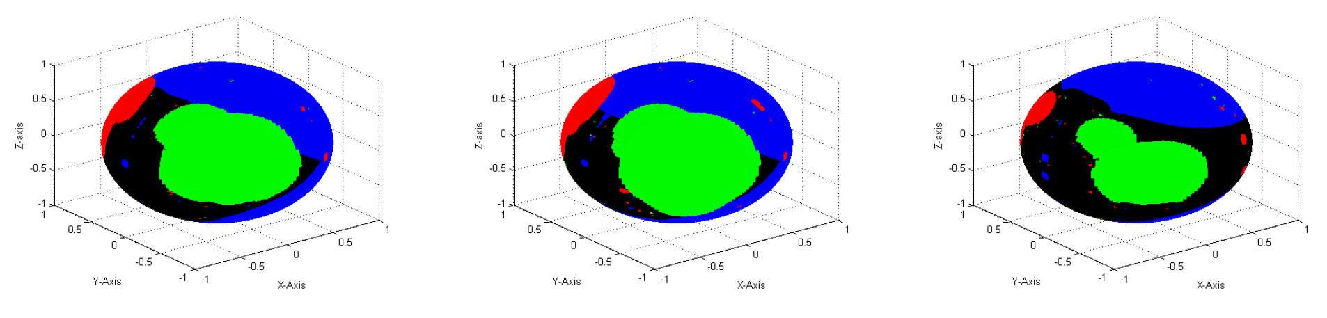
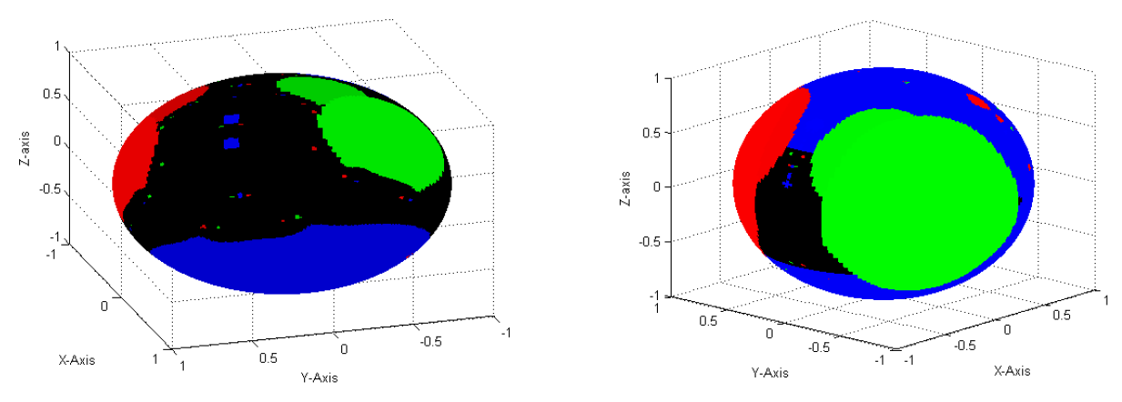
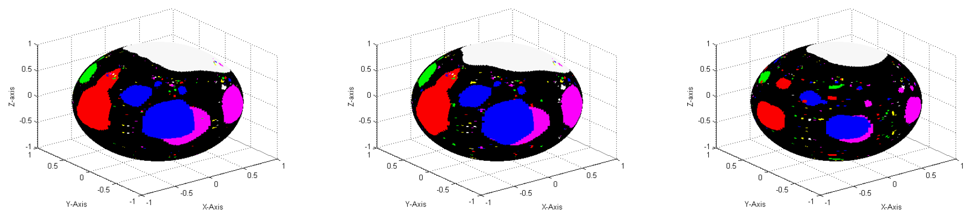
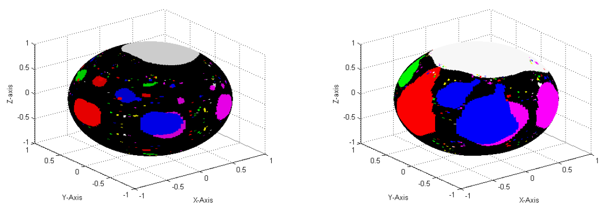
6. Stereographic Projection of Iterative Method without Memory

In this section, we analyzed the reliability of the iterative scheme through stereographic projection, which is a useful tool to provide us significant information about the convergence and stability of without-memory multipoint iterative schemes. This type of analysis has been performed by Andrew Nicklawsky [21].

Stereographic projection is a mapping between a sphere and a plane. The set of points on the surface of the sphere gives a complete representation in 3D space, the directions being the set of lines from the center of the sphere. It is defined as the unit sphere $U^2$ in 3D space, and $R^3$ is the set of points $\left(x,y,z\right)$ such that

$$U^2=\{\left(x,y,z\right)\in R^3|x^2+y^2+z^2=1\}\subset R^3.$$

For the stereographic projection, the transformation of the Cartesian coordinates is as follows:

$$\left(x,y,z\right)=(\frac{2X}{1+X^2+Y^2},\frac{2Y}{1+X^2+Y^2},\frac{-1+X^2+Y^2}{1+X^2+Y^2}).$$

The transformation of the Polar coordinates is as follows:

$$\left(r,\theta ,z\right)=\left(\frac{2R}{1+R^2},\ominus ,\frac{R^2-1}{R^2+1}\right).$$

The origin of the above two projections is $\left(0,0\right)$: the point $\left(0,0,-1\right)$ is on the south pole, the interior of the unit circle is mapped on the southern hemisphere, and the unit circle is mapped on the equator. The point $\left(0,0,1\right)$ is on the north pole, which is undefined but can be considered the manifestation of infinity as the points growing closer to it come from points in the plane increasingly distant from the origin. We take three complex polynomials to obtain the stereographic projection of different methods, which are

$$\begin{array}{ccc}\hfill r_1\left(z\right)& =& z^3-1.\hfill \\ \hfill r_2\left(z\right)& =& z^5-1.\hfill \\ \hfill r_3\left(z\right)& =& z^6-1.\hfill \end{array}$$

To generate the stereographic projection, we used a maximum of 60 iterations with 200 resolutions implemented in the computer programming language MATLAB R2014a. The roots of each polynomial are marked with different colors. $r_1\left(z\right)$ has three roots, so it can be seen from the stereographic images of $r_1\left(z\right)$ that three colors appeared, and these three colors reflect three roots, where the black color is used for divergence. The same holds in the case of $r_2\left(z\right)$, where five colors can be seen, and in the case of $r_3\left(z\right)$, where six colors of roots can be seen from the stereographic projections. If the sequence of root-finding iterative schemes converges in a smaller number of iterations, then the color will be bright, and if it is not converging to any of the roots, then the initial root is allotted with black color. In the following figures, we used a lower value of $-2$ and an upper value of 2 with an increment of $0.1$ on polynomials of 3rd, 5th, and 6th degree. The dynamical behavior of the newly proposed without-memory iterative schemes $\left(AK1\right)$ and $\left(AK2\right)$ and the known schemes without memory by Zafar et al. [13] $\left(FWM\right)$, Cordero et al. [18] $\left(M1\right)$, and Lotfi et al. [17] $\left(LM\right)$ are seen in Figure 1, Figure 2, Figure 3, Figure 4, Figure 5 and Figure 6.

Figure 1, Figure 2, Figure 3, Figure 4, Figure 5 and Figure 6 show the region of convergence and divergence through the stereographic projection of the developed families $\left(AK1\right)$ and $\left(AK2\right)$ compared with the existing families of the same domain. It can be seen from Figure 1 and Figure 2. that the newly developed methods AK1 and AK2 have wider and brighter regions of convergence and less regions of divergence as compared with FWM and M1, and their stability is comparable with LM in the case of $r_1\left(z\right).$ The same behavior can be observed from Figure 3 and Figure 4 in the case of polynomial $r_2\left(z\right)$ and Figure 5 and Figure 6 in the case of $r_3\left(z\right).$ Since the dynamical behavior of the presented families $\left(AK1\right)$ and $\left(AK2\right)$ have less black color in contrast with $\left(FWM\right)$ and $\left(M1\right)$, the stability and consistency of the newly proposed family is evident from the stereographic projection.

Without-memory iterative methods are algorithms that determine a subsequent iteration exclusively from the previous one. The current iteration, which is located on the sphere, can be converted to a point on the plane via stereographic projection. The next iterate is then obtained by applying the iteration process in the plane and projecting the resulting point back onto the sphere. This method can make the computation of iterates simpler, because working with points on a plane rather than a sphere may be simpler. Additionally, stereographic projection can show how iterates move on the sphere during the progress of an iteration, which can give geometric insight into how iterative techniques behave.

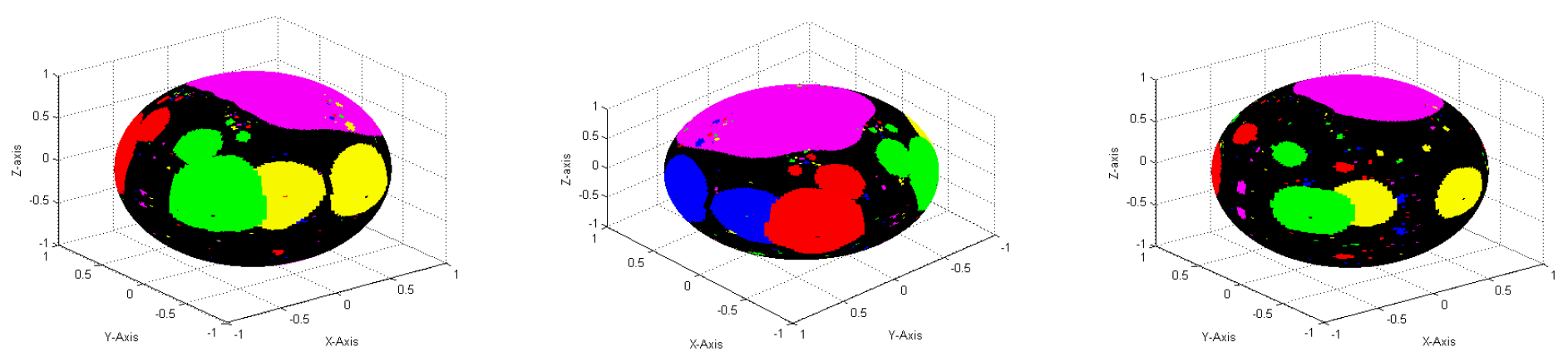
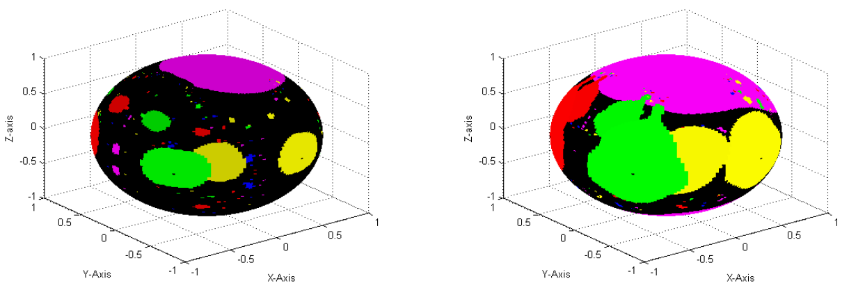
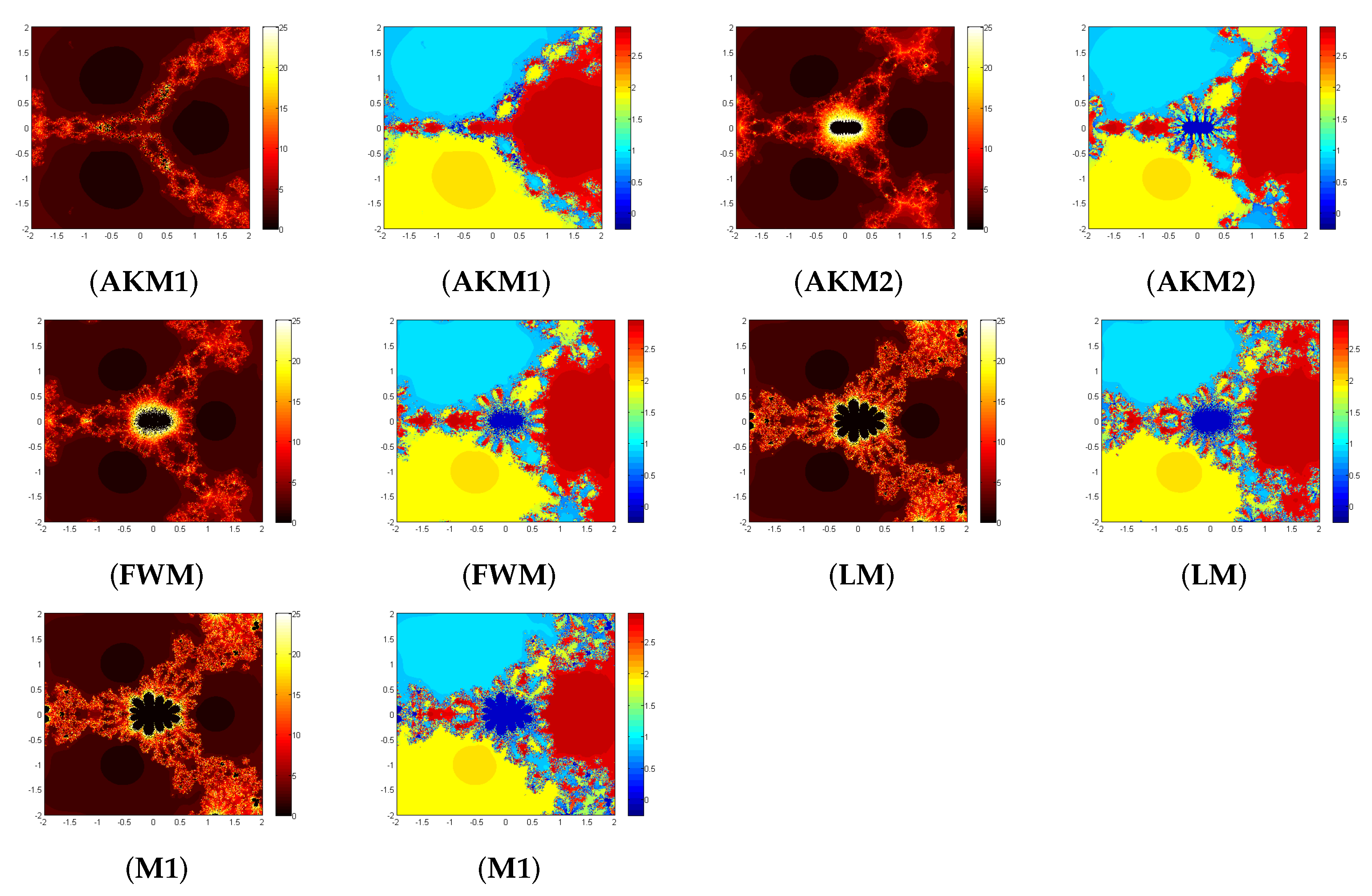
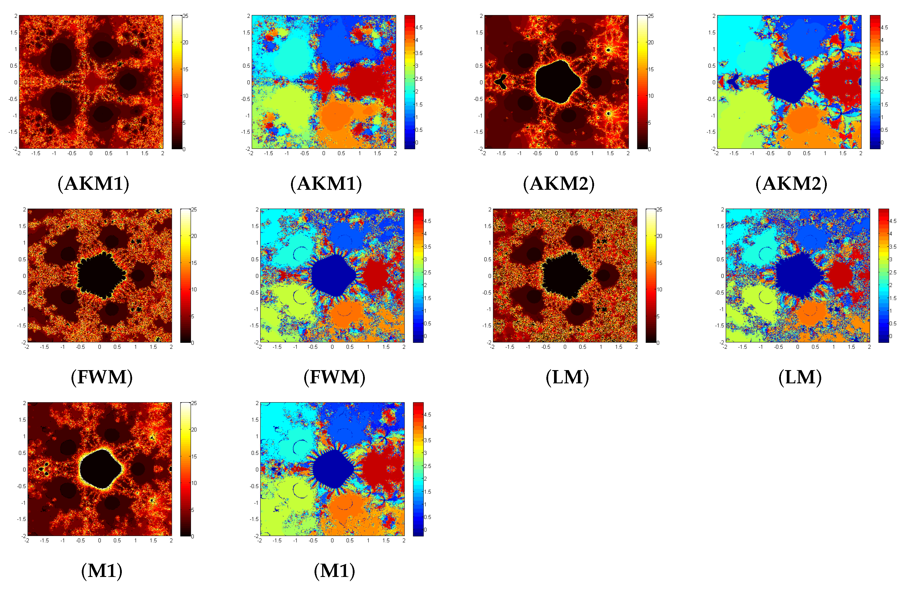
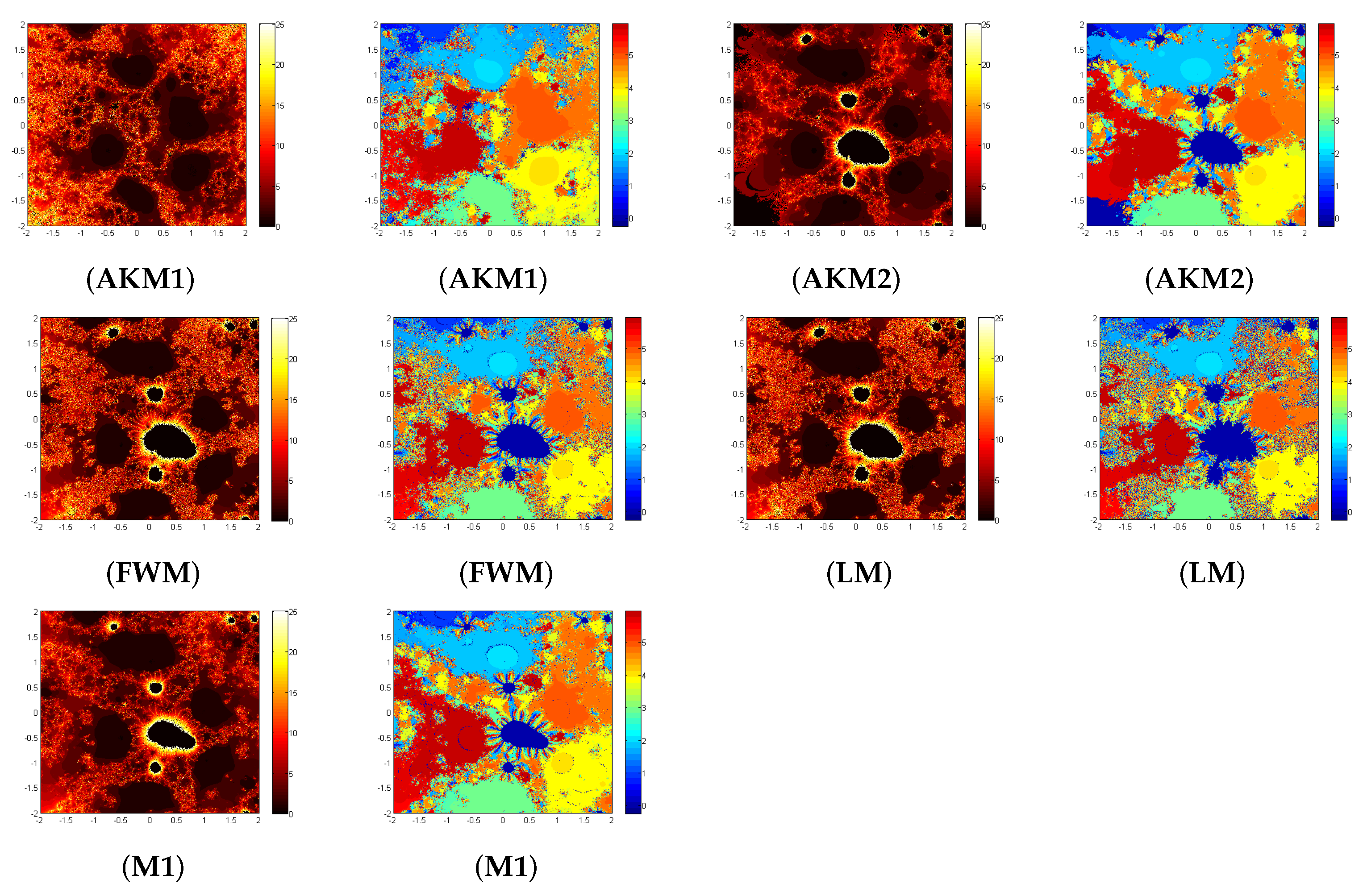
7. Dynamical Analysis of Iterative Methods with Memory

It is interesting to visualize the convergence region and stability of an iterative scheme through complex tools, such as symmetric basins of attraction and stereographic projections. The basic definitions and complex behavior of rational functions can be found in [22,23,24,25]. In the previous section, we investigated stereographic projections, and here, we analyze their symmetric basins of attractions for various iterative methods.

From a numerical viewpoint, complex properties of rational functions associated with iterative schemes give us significant information about their stability. To generate symmetric basins of attractions, we used two different scheme on Matlab R2014a. We consider a square box $B=\left[-2,2\right]\times \left[-2,2\right]\in C$ with $200\times 200$ grids. An initial approximation for the zero of a polynomial lies in the basins of attractions if an iterative method converges to it with stopping criterion; $\left|f\left({\xi }_m\right)\right|<{10}^{-5}$.

The first scheme assigns a specific shade to the initial points in order to visualize the convergence speed as a function of the number of iterations. Each initial point is assigned a unique color. If the iterative scheme’s sequence converges in fewer iterations, the color is brighter; if it does not converge to any of the roots after 30 iterations, the initial root is assigned a dark blue color. We use the same scale in the second method but assign a shade to each starting point based on the number of iterations required for the root-finding scheme to converge to any of the given function’s roots. We use a maximum of 25 iterations and the same stopping criteria as previously stated. If an iterative scheme does not converge within the specified number of iterations, it is said to be divergent for that particular starting point and is denoted by black shade. To generate symmetric basins of attractions (polynomiographs), we employ three complex functions, which are

$$\begin{array}{ccc}\hfill y_3\left(\xi \right)& =& {\xi }^3-1,\xi =1.0,-0.5000+0.86605I,-0.5000-0.86605I\hfill \\ \hfill y_5\left(\xi \right)& =& {\xi }^5-1,\xi =1.0,0.3090+0.95105I,-0.8090+0.58778I,\hfill \\ & & -0.8090-0.58778I,0.30902-0.95105I.\hfill \\ \hfill y_6\left(\xi \right)& =& {\xi }^6-\frac{1}{2}{\xi }^5+\frac{11\left(i+1\right)}{4}{\xi }^4-\frac{3i+19}{4}{\xi }^3+\frac{5i+11}{4}{\xi }^2+\frac{i-11}{4}\xi +\frac{3}{2}-3i,\hfill \\ \hfill \xi & =& -1.0068+2.0047i,0.0281+0.9963i,0.0279-1.5225i,\hfill \\ & & 1.0235-0.9556i,0.9557-0.0105i,-0.5284-0.5125i.\hfill \end{array}$$

The symmetric basins of attractions of the proposed with-memory schemes ($AKM1$) and ($AKM2$) and the existing methods with memory by Zafar et al. [13] $\left(FWM\right)$, Lotfi et al. [17] $\left(LM\right)$, and Cordero et al. [18] $\left(M1\right)$ are shown in Figure 7, Figure 8 and Figure 9.

According to Figure 7, Figure 8 and Figure 9, we conclude that with-memory methods (45) and (46), depending upon self-accelerating parameters calculated by (12), have the fastest order of convergence, as their convergence regions are darker and brighter than the other known schemes. Our methods $\left(AKM1\right)$ and $\left(AKM2\right)$ have wider convergence regions as compared with $\left(FWM\right)$, $\left(LM\right)$, and $\left(M1\right)$. Thus, the proposed schemes are more reliable and have better convergence regions than $\left(FWM\right)$, $\left(LM\right)$, and $\left(M1\right)$.

Additionally, the investigation of attraction basins can indicate the possibility of different solutions, which could have significant implications for the modeled system. In physics, for instance, the existence of numerous stable solutions can cause phase transitions, while in optimization problems, the existence of several solutions can point to the existence of local minima or maxima. In conclusion, the analysis of attraction basins offers a potential tool for comprehending the behavior of iterative approaches and enhancing their effectiveness. It can help professionals and researchers across a range of disciplines in more effectively and precisely resolving challenging issues.

8. Conclusions

In this paper, we developed a new family of optimal eighth-order derivative-free iterative method without memory for finding simple roots of nonlinear equations based on King’s scheme [2] and Lagrange interpolation. A convergence analysis is presented to show that the proposed method without memory has an optimal order of convergence of eight. Furthermore, we used four self-accelerating parameters and one variable’s weight function to extend the special cases $\left(AK1\right)$ and $\left(AK2\right)$ of the proposed family without memory to iterative schemes with memory, $\left(AKM1\right)$ and $\left(AKM2\right),$ without using additional function evaluations. We successfully increased the order of convergence from 8 to $15.51560$. The efficiency index of the proposed family without memory is increased from $1.6817$ to $1.9847$ without using additional functional evaluations. For the sake of comparison and implementation of the proposed and existing iterative schemes with and without memory, numerical results are presented using various test problems, including the eigenvalue problem, continuous stirred-tank reactor, and energy distribution for Planck’s radiation. Various dynamical approaches are presented to see the effectiveness of competitive iterative schemes: 3D stereographic projection in the case of iterative schemes without memory and 2D symmetric basins of attractions in the case of iterative schemes with memory. Such a rich analysis is rarely found in the literature. From both approaches, it is evident that our newly developed schemes are more stable, robust, and competent in their respective domains. Future research and analysis of the proposed scheme may be carried out in terms of stability and wide convergence zones in various domains. Visualizing the behavior of the iterative approaches may need looking into the usage of other graphical tools in addition to 2D symmetric basins of attraction and 3D stereographic projections.

References

1. Traub, J.F. Iterative Methods for the Solution of Equations; PrenticeHall, Inc.: Englewood Cliffs, NJ, USA, 1964. [Google Scholar]
2. King, R.F. A family of fourth order methods for non-linear equations. SIAM J. Numer. Anal. 1973, 10, 876–879. [Google Scholar] [CrossRef]
3. Ostrowski, A.M. Solution of Equations and System of Equations; Academic Press: New York, NY, USA, 1960. [Google Scholar]
4. Kung, H.T.; Traub, J.F. Optimal order of one point and multipoint iteration. J. Assoc. Comput. Math. 1974, 21, 643–651. [Google Scholar] [CrossRef]
5. Steffensen, I.F. Remarks on iteration. Skand. Aktuarietidskr. 1933, 16, 64–72. [Google Scholar] [CrossRef]
6. Akram, S.; Zafar, F.; Junjua, M.D.; Yasmin, N. A general family of derivative free with and without memory root finding methods. JPRM 2020, 16, 64–83. [Google Scholar]
7. Džunić, J.; Petković, M.S. On generalized multipoint root-solvers with memory. Comput. Appl. Math. 2012, 236, 2909–2920. [Google Scholar] [CrossRef]
8. Junjua, M.D.; Zafar, F.; Yasmin, N.; Akram, S. A general class of derivative free root solvers with-memory. U.P.B. Sci. Bull. Ser. A 2017, 79, 19–28. [Google Scholar]
9. Lotfi, T.; Soleymani, F.; Ghorbanzadeh, M.; Assari, P. On the construction of some tri-parametric iterative methods with memory. Numer. Algorithms 2015, 70, 835–845. [Google Scholar] [CrossRef]
10. Petković, M.S.; Neta, B.; Petković, L.D.; Džunić, J. Multipoint Methods for Solving Nonlinear Equations; Elsevier: Amsterdam, The Netherlands, 2013. [Google Scholar]
11. Petković, M.S.; Neta, B.; Petković, L.D.; Džunić, J. Multipoint methods for solving nonlinear equations: A survey. Appl. Math. Comput. 2014, 226, 635–660. [Google Scholar] [CrossRef]
12. Solaiman, O.S.; Ariffin, S.; Karim, A.; Hashimc, I. Optimal fourth- and eighth-order of convergence derivative-free modifications of King’s method. J. King Saud Univ.-Sci. 2019, 31, 1499–1504. [Google Scholar] [CrossRef]
13. Zafar, F.; Akram, S.; Yasmin, N.; Junjua, M. On the construction of three step four parametric methods with accelerated order of convergence. J. Nonlinear Sci. Appl. 2016, 9, 4542–4553. [Google Scholar] [CrossRef]
14. Zafar, F.; Cordero, A.; Torregrosa, J.R.; Ra, A. A class of four parametric with- and without-memory root finding methods. Comput. Math. Methods 2019, 1, e1024. [Google Scholar] [CrossRef]
15. Zafar, F.; Yasmin, N.; Kutbi, M.A.; Zeshan, M. Construction of tri-parametric derivative free fourth order with and without memory iterative method. J. Nonlinear Sci. Appl. 2016, 9, 1410–1423. [Google Scholar] [CrossRef]
16. Petkovic, M.S.; Zunic, J.; Petkovic, L.D. A family of two point methods with-memory for solving nonlinear equations. Appl. Anal. Discret. Math. 2011, 5, 298–317. [Google Scholar] [CrossRef]
17. Lotfi, T.; Assari, P. New three- and four-parametric iterative with-memory methods with efficiency index near 2. Appl. Math. Comput. 2015, 270, 1004–1010. [Google Scholar] [CrossRef]
18. Cordero, A.; Janjua, M.; Torregrosa, J.R.; Yasmin, N.; Zafar, F. Efficient four parametric with and without-memory iterative methods possessing high efficiency indices. Math. Prob. Eng. 2018, 2018, 8093673. [Google Scholar] [CrossRef]
19. Behl, R.; Zafar, F.; Alshormani, A.S.; Junjua, M.; Yasmin, N. An Optimal Eighth-Order Scheme for Multiple Zeros of Univariate Functions. Int. J. Comput. Methods 2019, 16, 1843002. [Google Scholar] [CrossRef]
20. Douglas, J.M. Process Dynamics and Control; Prentice Hall: Englewood Cliffs, NJ, USA, 1972. [Google Scholar]
21. Nicklawsky, A. Visualizing Chaos. Mathematics Student Work. 1. 2012. Available online: https://digitalcommons.csbsju.edu/math_students/1 (accessed on 13 May 2023).
22. Amat, S.; Busquier, S.; Bermúdez, C.; Magrenan, A.A. On the election of the damped parameter of a two-step relaxed Newton-type method. Nonlinear Dyn. 2016, 84, 9–18. [Google Scholar] [CrossRef]
23. Chun, C.; Neta, B. Comparing the basins of attraction for KANwar-Bhatia-Kansal family to the best fourth order method. Appl. Math. Comput. 2015, 266, 277–292. [Google Scholar] [CrossRef]
24. Sharma, J.R.; Kumar, S. Efficient methods of optimal eighth and sixteenth order convergence for solving nonlinear equations. SeMA 2018, 75, 229–253. [Google Scholar] [CrossRef]
25. Neta, B.; Chun, C.; Scott, M. Basins of attraction for optimal eighth order methods to find simple roots of nonlinear equations. Appl. Math. Comput. 2014, 227, 567–592. [Google Scholar] [CrossRef]
Figure 1. Stereographic projection of AK1 (left), AK2 (middle), and FWM (right) on r 1 (z).
Symmetry 15 01116 g001
Figure 2. Stereographic projection of M1 (left) and LM (Right) on r 1 (z).
Symmetry 15 01116 g002
Figure 3. Stereographic projection of AK1 (left), AK2 (middle), and FWM (right) on r 2 (z).
Symmetry 15 01116 g003
Figure 4. Stereographic projection of M1 (left) and LM (right) on r 2 (z).
Symmetry 15 01116 g004
Figure 5. Stereographic projection of AK1 (left), AK2 (middle), and FWM (right) on r 3 (z).
Symmetry 15 01116 g005
Figure 6. Stereographic projection of M1 (left) and LM (right) on r 3 (z).
Symmetry 15 01116 g006
Figure 7. The convergence regions of different methods with memory for y 3 ( ξ ) .
Symmetry 15 01116 g007
Figure 8. The convergence regions of different methods with memory for y 5 ( ξ ) .
Symmetry 15 01116 g008
Figure 9. The convergence regions of different methods with memory for y 6 ( ξ ) .
Symmetry 15 01116 g009