Properties of Differential Equations Related to Degenerate q-Tangent Numbers and Polynomials

Abstract

In this paper, we construct degenerate q-tangent numbers and polynomials and determine their related properties. Based on these numbers and polynomials, we also confirm that the structure of the approximate root changes according to changes in q and h. We find differential equations that have degenerate q-tangent polynomials as solutions and also find differential equations that have other polynomials as coefficients, confirming the relationships among these.

1. Introduction

Before clarifying the objectives of this paper, it is necessary to introduce the basic concepts. Hence, we first identify several definitions and properties needed to understand this paper. Let $n,q\in \mathbb{R}$ with $q\ne 1$. The quantum number or q-number discovered by Jackson is

$${\left[n\right]}_q=\frac{1-q^n}{1-q},$$

noting that ${lim}_{q\to 1}{\left[n\right]}_q=n$. In particular, for $k\in \mathbb{Z}$, where ${\left[k\right]}_q$ is called the q-integer [1,2,3].

Many mathematicians have researched the use of q-numbers in multiple fields such as q-discrete distributions, q-differential equations, q-series, and q-calculus [4,5,6].

The equation

$${\left[\begin{array}{c}m\\ r\end{array}\right]}_q=\frac{{\left[m\right]}_q!}{{[m-r]}_q!{\left[r\right]}_q!},$$

defines the q-Gaussian binomial coefficients, where m and r are non-negative integers [3,5]. For $r=0$, the coefficient value is 1 since the numerator and denominator are both empty products. Therefore, ${\left[n\right]}_q!={\left[n\right]}_q{[n-1]}_q\cdots {\left[2\right]}_q{\left[1\right]}_q$ and ${\left[0\right]}_q!=1$.

Consider an arbitrary function $f\left(x\right)$. Its q-differential is

$$d_{q}f\left(x\right)=f\left(qx\right)-f\left(x\right),$$

and its h-differential is

$$d_{h}f\left(x\right)=f(x+h)-f\left(x\right).$$

In particular, we note $d_{q}x=(q-1)x$ and $d_{h}x=h$. An difference between the quantum differentials and the ordinary ones is the lack of symmetry in the differential of the product of two functions. Since

$$\begin{array}{ll}{d}_q\left(f\left(x\right)g\left(x\right)\right)& =f\left(qx\right)g\left(qx\right)-f\left(x\right)g\left(x\right)\\ & =f\left(qx\right)g\left(qx\right)-f\left(qx\right)g\left(x\right)+f\left(qx\right)g\left(x\right)-f\left(x\right)g\left(x\right),\end{array}$$

we have

$$d_q\left(f\left(x\right)g\left(x\right)\right)=f\left(qx\right)d_{q}g\left(x\right)+g\left(x\right)d_{q}f\left(x\right),$$

and similarly,

$$d_h\left(f\left(x\right)g\left(x\right)\right)=f(x+h)d_{h}g\left(x\right)+g\left(x\right)d_{h}f\left(x\right).$$

The following two quantum derivatives:

$$\begin{gathered} D_{q}f\left(x\right)=\frac{d_{q}f\left(x\right)}{d_{q}x}=\frac{f\left(qx\right)-f\left(x\right)}{(q-1)x}, \\ {D}_{h}f\left(x\right)=\frac{d_{h}f\left(x\right)}{d_{h}x}=\frac{f(x+h)-f\left(x\right)}{h}, \end{gathered}$$

are called the q-derivative and h-derivative, respectively, of the function $f\left(x\right)$. We note ${lim}_{q\to 1}{D}_{q}f\left(x\right)={lim}_{h\to 0}{D}_{h}f\left(x\right)=\frac{df\left(x\right)}{dx}$ if $f\left(x\right)$ is differentiable [3].

In ref. [7], a two-parameter time scale ${\mathbf{T}}_{q,h}$ was introduced as follows:

$${\mathbf{T}}_{q,h}:=\{q^{n}x+{\left[n\right]}_{q}h|x\in \mathbb{R},n\in \mathbb{Z},h,q\in {\mathbb{R}}^{+},q\ne 1\}\cup \left\{\frac{h}{1-q}\right\}.$$

Definition 1

([7,8]). Let $f:{\mathbf{T}}_{q,h}\to \mathbb{R}$ be any function. Thus, the delta $(q,h)$-derivative of f $D_{q,h}\left(f\right)$ is defined by

$$D_{q,h}f\left(x\right):=\frac{f(qx+h)-f\left(x\right)}{(q-1)x+h}.$$

From the above definition, we identify several properties as follows:

(i)

$D_{q,h}f\left(x\right)=0$ if $f\left(x\right)$ is constant.

(ii)

$D_{q,h}f\left(x\right)=D_{q,h}g\left(x\right)$ for all $x\in \mathbb{R}$ if $f\left(x\right)=g\left(x\right)+c$ with some constant c.

(iii)

$D_{q,h}f\left(x\right)=c_1$ if $f\left(x\right)=c_{1}x+c_2$, where $c_1$ and $c_2$ are constant.

In Definition 1, we can see $D_{q,h}\left(f\right)$, the delta $(q,h)$-derivative of f is reduced to $D_q\left(f\right)$, the q-derivative of f for $h=0$ reduces to $D_h\left(f\right)$, and the h-derivative of f for $q\to 1$. In addition, we can derive the product and quotient rules for the delta $(q,h)$-derivative.

The q-analogue of binomial ${(x-a)}^n$ is

$${(x-a)}_q^n=\left\{\begin{array}{c}1\mathrm{if}n=0,\hfill \\ (x-a)(x-qa)\cdots (x-q^{n-1}a)\mathrm{if}n\ge 1.\hfill \end{array}\right.$$

For any positive integer n, we note that ${(x-a)}_q^{m+n}={(x-a)}_q^m{(x-q^{m}a)}_q^n$ and ${(x-a)}_q^{-n}=\frac{1}{{(x-q^{-n}a)}_q^n}$. For $n\ge 1$, the h-analogue of binomial ${(x-a)}^n$ is

$${(x-a)}_h^n=(x-a)(x-a-h)\cdots (x-a-(n-1)h),$$

and ${(x-a)}_h^0=1$. Similar to the q-version, we note ${(x-a)}_h^{m+n}={(x-a)}_h^n{(x-a-nh)}_h^m$ and ${(x-a)}_q^{-n}=\frac{1}{{(x-a+nh)}_q^n}$ [3].

Definition 2

([8,9]). The generalized quantum binomial ${(x-x_0)}_{q,h}^n$ is defined by

$${(x-x_0)}_{q,h}^n:=\left\{\begin{array}{cc}1,& \mathrm{if} n=0,\hfill \\ \prod _{i=1}^n\left(x-(q^{i-1}{x}_0+{[i-1]}_{q}h)\right),& \mathrm{if} n>0,\hfill \end{array}\right.$$

where $x_0\in \mathbb{R}$.

The generalized quantum binomial reduces to the q-analogue of binomial ${(x-x_0)}_q^n$ as $h\to 0$ and to the h-analogue of binomial ${(x-x_0)}_h^n$ as $q\to 1$. Furthermore, we note that ${lim}_{(q,h)\to (1,0)}{(x-x_0)}_{q,h}^n={(x-x_0)}^n$.

A q-analogue of the classical exponential function (q-exponential function) is

$$e_q\left(x\right)=\sum _{n=0}^{\infty }\frac{x^n}{{\left[n\right]}_q!}.$$

We can find another q-analogue of the classical exponential function $E_q\left(x\right)=e_{q^{-1}}\left(x\right)$. Its two q-analogues have similar behavior such as $D_q{e}_q\left(x\right)=e_q\left(x\right)$ and $D_q{E}_q\left(x\right)=E_q\left(qx\right)$.

The h-analogue of the classical exponential function (h-exponential function) is

$$e_h\left(x\right)={(1+h)}^{\frac{x}{h}}.$$

In particular, $e_1\left(x\right)=2^x$. As $h\to 0$, the base ${(1+h)}^{\frac{1}{h}}$ approaches e, as expected [3].

Definition 3

([8]). The generalized quantum exponential function ${\exp }_{q,h}\left(\alpha x\right)$ is defined as

$${\exp }_{q,h}\left(\alpha x\right):=\sum _{i=0}^{\infty }\frac{{\alpha }^i{(x-0)}_{q,h}^i}{{\left[i\right]}_q!},$$

where α is an arbitrary non-zero constant.

Clearly, we note that ${\exp }_{q,h}\left(0\right)=1$. As $h\to 0$ with $\alpha =1$, the generalized quantum exponential function ${\exp }_{q,h}\left(\alpha x\right)$ becomes the so-called q-exponential function $e_q\left(x\right)$ [3,5]. Likewise, as $q\to 1$ with $\alpha =1$, the generalized quantum exponential function ${\exp }_{q,h}\left(\alpha x\right)$ reduces to the so-called h-exponential function $e_{1,h}\left(x\right)={(1+h)}^{\frac{x}{h}}$ [3].

Based on the above concept, many mathematicians have studied q-special functions, q-differential equations, q-calculus, and so on (see [6,10,11,12,13,14,15]). For example, Duran, Acikgoz, and Araci [16] considered different types of trigonometric functions and hyperbolic functions related to quantum numbers and looked for properties related to them. Mathematicians have also proven various theorems related to basic concepts based on h-numbers. Benaoum [9] obtained Newton’s binomial formula relating to $(q,h)$, while Cermak and Nechvatal [7] derived a $(q,h)$ version of the fractional calculus. In 2011, Rahmat [17] studied the $(q,h)$-Laplace transform, while in 2019, Silindir and Yantir [8] studied the generalization of quantum Taylor formula and quantum binomial. Their results motivated the current research presented in this paper. Defining and characterizing degenerate tangent polynomials, mathematicians are now curious about their definition and properties when combined with quantum numbers. Roo and Kang [18] studied some properties for q-special polynomials and observed approximate roots of q-Euler and q-Genocchi polynomials.

The main purpose of this paper is to construct degenerate q-tangent polynomials. Based on the constructed polynomials, we formulate differential equations and investigate their properties. This paper discusses the properties of series combined with quantum numbers and their generalization.

The results present here may be useful to researchers studying quantum physics, non-linear physics, and non-linear differential equations.

Definition 4

([13,19]). The q-tangent numbers and polynomials are defined as

$$\sum _{n=0}^{\infty }{T}_{n,q}\frac{t^n}{{\left[n\right]}_q!}=\frac{2}{e_q\left(2t\right)+1},\sum _{n=0}^{\infty }{T}_{n,q}\left(x\right)\frac{t^n}{{\left[n\right]}_q!}=\frac{2}{e_q\left(2t\right)+1}{e}_q\left(tx\right).$$

For $q\to 1$, we note that q-tangent numbers and polynomials become tangent numbers and polynomials, respectively.

Definition 5

([20]). The degenerate tangent numbers and polynomials are defined as

$$\sum _{n=0}^{\infty }{T}_{n,\lambda }\frac{t^n}{n!}=\frac{2}{{(1+\lambda t)}^{\frac{2}{\lambda }}+1},\sum _{n=0}^{\infty }{T}_{n,\lambda }\left(x\right)\frac{t^n}{n!}=\frac{2}{{(1+\lambda t)}^{\frac{2}{\lambda }}+1}{(1+\lambda t)}^{\frac{x}{\lambda }}.$$

As $h\to 0$ in Definition 5, we note that degenerate tangent numbers and polynomials become tangent numbers and polynomials, respectively.

In this paper, we define degenerate q-tangent numbers and polynomials, findings several properties of these polynomials by using q-numbers, and $(q,h)$-derivatives. In addition, we construct several higher-order differential equations whose solutions are degenerate q-tangent polynomials.

2. Differential Equations for Degenerate $\mathbf{q}$-Tangent Polynomials

In this section, we define degenerate q-tangent numbers and polynomials using degenerate q-exponential functions. Using the $(q,h)$-derivative, we obtain several differential equations related to degenerate q-tangent polynomials. Furthermore, we find relations among q-tangent polynomials, degenerate tangent polynomials, and degenerate q-tangent polynomials.

Here, we introduce the degenerate quantum exponential function.

$$e_{q,h}(x:t):=\sum _{n=0}^{\infty }{\left(x\right)}_{q,h}^n\frac{t^n}{n!}=\sum _{n=0}^{\infty }{(x-0)}_{q,h}^n\frac{t^n}{n!}$$

Setting $x=2$, we have

$$e_{q,h}(2:t)=\sum _{n=0}^{\infty }{\left(2\right)}_{q,h}^n\frac{t^n}{n!},$$

where ${\left(2\right)}_{q,h}^n={(2-0)}_{q,h}^n=2(2-h)\cdots (2-{[n-1]}_{q}h)$.

From the property of $e_{q,h}(x:t)$, we note the relation

$$\begin{array}{ll}{e}_{q,h}(qx:t)& ={\displaystyle \sum _{n=0}^{\infty }}qx(qx-h)(qx-{\left[2\right]}_{q}h)(qx-{\left[3\right]}_{q}h)\cdots (qx-{[n-1]}_{q}h)\frac{t^n}{{\left[n\right]}_q!}\\ & =e_{q,q^{-1}h}(x:qt).\end{array}$$

(1)

Definition 6.

Let $\left|q\right|<1$ and h be a non-negative integer. Then, we can define the degenerate q-tangent polynomial $T_{n,q}(x:h)$ as

$$\sum _{n=0}^{\infty }{T}_{n,q}(x:h)\frac{t^n}{{\left[n\right]}_q!}=\frac{2}{e_{q,h}(2:t)+1}{e}_{q,h}(x:t).$$

For $x=0$ in Definition 6, we note that

$$\sum _{n=0}^{\infty }{T}_{n,q}(0:h)\frac{t^n}{{\left[n\right]}_q!}:=\sum _{n=0}^{\infty }{T}_{n,q}\left(h\right)\frac{t^n}{{\left[n\right]}_q!}=\frac{2}{e_{q,h}(2:t)+1},$$

where $T_{n,q}\left(h\right)$ are called degenerate q-tangent numbers. From Definition 6, we can see certain relations between the tangent, degenerate tangent, and $(p,q)$-tangent polynomials. Setting $h\to 0$ in Definition 6, we can derive the q-tangent numbers $T_{n,q}$ and polynomials $T_{n,q}\left(x\right)$ as follows:

$$\sum _{n=0}^{\infty }{T}_{n,q}\frac{t^n}{{\left[n\right]}_q!}=\frac{2}{e_q\left(2t\right)+1},\sum _{n=0}^{\infty }{T}_{n,q}\left(x\right)\frac{t^n}{{\left[n\right]}_q!}=\frac{2}{e_q\left(2t\right)+1}{e}_q\left(tx\right).$$

As $h\to 0$ and $q\to 1$ in Definition 6, we obtain the tangent numbers $T_n$ and polynomials $T_n\left(x\right)$

$$\sum _{n=0}^{\infty }{T}_n\frac{t^n}{n!}=\frac{2}{e^{2t}+1},\sum _{n=0}^{\infty }{T}_n\left(x\right)\frac{t^n}{n!}=\frac{2}{e^{2t}+1}{e}^{tx}.$$

When $q\to 1$ in Definition 6, we can recover the degenerate tangent numbers $T_n\left(h\right)$ and polynomials $T_n(x:h)$ as follows:

$$\sum _{n=0}^{\infty }{T}_n\left(h\right)\frac{t^n}{n!}=\frac{2}{{(1+ht)}^{\frac{2}{h}}+1},\sum _{n=0}^{\infty }{T}_n(x:h)\frac{t^n}{n!}=\frac{2}{{(1+ht)}^{\frac{2}{h}}+1}{(1+ht)}^{\frac{x}{h}},$$

where $T_n\left(h\right)=T_n(0:h)$.

Here is a list of some degenerate q-tangent numbers:

$$\begin{array}{ll}{T}_{0,q}\left(h\right)& =1,\\ T_{1,q}\left(h\right)& =0,\\ T_{2,q}\left(h\right)& =-1+h,\\ T_{3,q}\left(h\right)& =-(-1+h+q)(-2+h+(-1+h)q),\\ T_{4,q}\left(h\right)& =-3+h^3(1+q)(1+q+q^2)+q(3+q(4+2q-q^3))\\ & +h(6+q+q^2(-5+q(-6+(-3+q)q)))\\ & +h^2(-4+q(-5+q(-2+q+2q^2))),\\ & \cdots .\end{array}$$

Several degenerate q-tangent polynomials are as follows:

$$\begin{array}{ll}{T}_{0,q}(x:h)& =1,\\ T_{1,q}(x:h)& =-1+x,\\ T_{2,q}(x:h)& =-1+h+q-(1+h+q)x+x^2,\\ T_{3,q}(x:h)& =-(1+q)(1+h^2+2h(-1+q)+(-3+q)q)\\ & +(-1+q^3+h^2(1+q)+2h(1+q+q^2))x\\ & -(1+q+q^2+h(2+q))x^2+x^3,\\ & \cdots .\end{array}$$

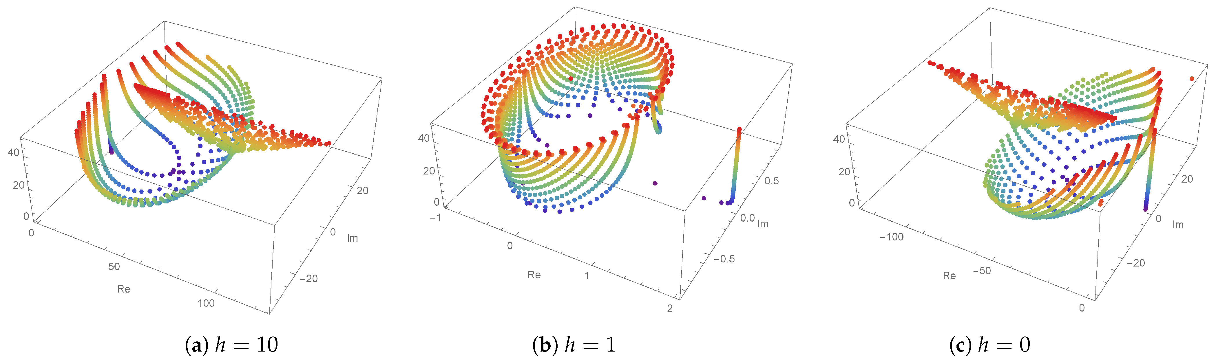
Figure 1 shows the structure of the approximate roots of degenerate q-tangent polynomials. Here, we impose the conditions $0\le n\le 50$ and $q=0.1$. Figure 1a,b show the structure of the approximate roots for $h=40$ and $h=0$, respectively. The approximate structure of degenerate q-tangent polynomials when h is $-40$ is shown in Figure 1c.

Theorem 1.

For $\left|q\right|<1$ and $h\in \mathbb{N}$, we have

$$D_{q,h,x}^{\left(1\right)}{T}_{n,q}(x:h)={\left[n\right]}_q{T}_{n-1,q}(x:h).$$

Proof. 

From generating the function of the degenerate q-tangent polynomials $T_{n,q}(x:h)$, we obtain

$$\begin{array}{ll}{\displaystyle \sum _{n=0}^{\infty }}{T}_{n,q}(x:h)\frac{t^n}{{\left[n\right]}_q!}& ={\displaystyle \sum _{n=0}^{\infty }}{T}_{n,q}\left(h\right)\frac{t^n}{{\left[n\right]}_q!}{\displaystyle \sum _{n=0}^{\infty }}{\left(x\right)}_{q,h}^n\frac{t^n}{{\left[n\right]}_q!}\\ & ={\displaystyle \sum _{n=0}^{\infty }}\left({\displaystyle \sum _{k=0}^n}\frac{{\left[n\right]}_q!}{{[n-k]}_q!{\left[k\right]}_q!}{\left(x\right)}_{q,h}^{n-k}{T}_{k,q}\left(h\right)\right)\frac{t^n}{{\left[n\right]}_q!}.\end{array}$$

From this equation, we can establish the relation between the degenerate q-tangent polynomials and degenerate q-tangent numbers as follows:

$$T_{n,q}(x:h)=\sum _{k=0}^n{\left[\begin{array}{c}n\\ k\end{array}\right]}_q{\left(x\right)}_{q,h}^{n-k}{T}_{k,q}\left(h\right).$$

(2)

Using the $(q,h)$-derivative in Equation (2), we can derive the following equation:

$$\begin{array}{ll}{D}_{q,h,x}^{\left(1\right)}{T}_{n,q}(x:h)& ={\displaystyle \sum _{k=0}^n}{\left[\begin{array}{c}n\\ k\end{array}\right]}_q{[n-k]}_q{\left(x\right)}_{q,h}^{n-k-1}{T}_{k,q}\left(h\right)\\ & ={\left[n\right]}_q{T}_{n-1,q}(x:h).\end{array}$$

This completes the proof.  □

Corollary 1.

Let k be a non-negative integer. From Theorem 1, the following holds:

$$T_{n-k,q}(x:h)=\frac{{[n-k]}_q!}{{\left[n\right]}_q!}{D}_{q,h,x}^{\left(k\right)}{T}_{n,q}(x:h).$$

Corollary 2.

(i) Letting $q\to 1$ in Theorem 1, we have

$$D_{h,x}^{\left(1\right)}{T}_n(x:h)=n{T}_{n-1}(x:h),T_{n-k}(x:h)=\frac{(n-k)!}{n!}{D}_{h,x}^{\left(k\right)}{T}_n(x:h),$$

where $D_h$ is the h-derivative and $T_{n,h}\left(x\right)$ are the degenerate tangent polynomials.

(ii) Letting $h\to 0$ in Theorem 1, we have

$$D_{q,x}^{\left(1\right)}{T}_{n,q}\left(x\right)={\left[n\right]}_q{T}_{n-1,q}\left(x\right),T_{n-k,q}\left(x\right)=\frac{{[n-k]}_q!}{{\left[n\right]}_q!}{D}_{q,x}^{\left(k\right)}{T}_{n,q}\left(x\right),$$

where $D_q$ is the q-derivative and $T_{n,q}\left(x\right)$ are q-tangent polynomials.

Theorem 2.

The solutions following differential equation

$$\begin{gathered} \frac{{\left(2\right)}_{q,h}^n}{{\left[n\right]}_q!}{D}_{q,h,x}^{\left(n\right)}{T}_{n,q}(x:h)+\frac{{\left(2\right)}_{q,h}^{n-1}}{{[n-1]}_q!}{D}_{q,h,x}^{(n-1)}{T}_{n,q}(x:h)+\frac{{\left(2\right)}_{q,h}^{n-2}}{{[n-2]}_q!}{D}_{q,h,x}^{(n-2)}{T}_{n,q}(x:h) \\ +\cdots +\frac{{\left(2\right)}_{q,h}^2}{{\left[2\right]}_q!}{D}_{q,h,x}^{\left(2\right)}{T}_{n,q}(x:h)+2D_{q,h,x}^{\left(1\right)}{T}_{n,q}(x:h)+2T_{n,q}(x:h)-2{\left(x\right)}_{q,h}^n=0, \end{gathered}$$

are degenerate q-tangent polynomials.

Proof. 

Suppose that $e_{q,h}(2:t)\ne -1$ in the generating function of the degenerate q-tangent polynomials. Then, we have

$$\sum _{n=0}^{\infty }{T}_{n,q}(x:h)\frac{t^n}{{\left[n\right]}_q!}\left(e_{q,h}(2:t)+1\right)=2e_{q,h}(x:t).$$

(3)

The left-hand side of Equation (3) transforms to

$$\begin{array}{l}{\displaystyle \sum _{n=0}^{\infty }}{T}_{n,q}(x:h)\frac{t^n}{{\left[n\right]}_q!}\left(e_{q,h}(2:t)+1\right)\\ ={\displaystyle \sum _{n=0}^{\infty }}\left({\displaystyle \sum _{k=0}^n}{\left[\begin{array}{c}n\\ k\end{array}\right]}_q{\left(2\right)}_{q,h}^k{T}_{n-k,q}(x:h)+T_{n,q}(x:h)\right)\frac{t^n}{{\left[n\right]}_q!}\end{array}$$

while the right-hand side becomes

$$2e_{q,h}(x:t)=2\sum _{n=0}^{\infty }{\left(x\right)}_{q,h}^n\frac{t^n}{{\left[n\right]}_q!}$$

Hence, we derive

$$\sum _{k=0}^n{\left[\begin{array}{c}n\\ k\end{array}\right]}_q{\left(2\right)}_{q,h}^k{T}_{n-k,q}(x:h)+T_{n,q}(x:h)=2{\left(x\right)}_{q,h}^n.$$

(4)

Considering Corollary 1 in Equation (4), we obtain

$$\sum _{k=0}^n\frac{{\left(2\right)}_{q,h}^k}{{\left[k\right]}_q!}{D}_{q,h,x}^{\left(k\right)}{T}_{n,q}(x:h)+T_{n,q}(x:h)-2{\left(x\right)}_{q,h}^n=0.$$

Therefore, we obtain the desired result.  □

Corollary 3.

Letting $q\to 1$ in Theorem 2, we have

$$\begin{gathered} \frac{{\left(2\right)}_{1,h}^n}{n!}{D}_{h,x}^{\left(n\right)}{T}_n(x:h)+\frac{{\left(2\right)}_{1,h}^{n-1}}{(n-1)!}{D}_{h,x}^{(n-1)}{T}_n(x:h)+\frac{{\left(2\right)}_{1,h}^{n-2}}{(n-1)!}{D}_{h,x}^{(n-2)}{T}_n(x:h) \\ +\cdots +\frac{{\left(2\right)}_{1,h}^2}{2!}{D}_{h,x}^{\left(2\right)}{T}_n(x:h)+2D_{h,x}^{\left(1\right)}{T}_n(x:h)+2T_n(x:h)-2{\left(x\right)}_{1,h}^n=0, \end{gathered}$$

where $D_h$ is the h-derivative and $T_n(x:h)$ are degenerate tangent polynomials.

Corollary 4.

Letting $h\to 0$ in Theorem 2, the following holds:

$$\begin{array}{l}\frac{2}{{\left[n\right]}_q!}{D}_{q,x}^{\left(n\right)}{T}_{n,q}\left(x\right)+\frac{2}{{[n-1]}_q!}{D}_{q,x}^{(n-1)}{T}_{n,q}\left(x\right)+\frac{2}{{[n-2]}_q!}{D}_{q,x}^{(n-2)}{T}_{n,q}\left(x\right)+\cdots \\ +\frac{2}{{\left[2\right]}_q!}{D}_{q,x}^{\left(2\right)}{T}_{n,q}\left(x\right)+2D_{q,x}^{\left(1\right)}{T}_{n,q}\left(x\right)+2T_{n,q}\left(x\right)-2x^n=0,\end{array}$$

where $D_q$ is the q-derivative and $T_{n,q}\left(x\right)$ are q-tangent polynomials.

Theorem 3.

The degenerate q-tangent polynomials are solutions of the following differential equation:

$$\begin{array}{l}\frac{T_{n,q}(2:h)+T_{n,q}\left(h\right)}{{\left[n\right]}_q!}{D}_{q,h,x}^{\left(n\right)}{T}_{n,q}(x:h)+\frac{T_{n-1,q}(2:h)+T_{n-1,q}\left(h\right)}{{[n-1]}_q!}{D}_{q,h,x}^{(n-1)}{T}_{n,q}(x:h)+\cdots \\ +\frac{T_{2,q}(2:h)+T_{2,q}\left(h\right)}{{\left[2\right]}_q!}{D}_{q,h,x}^{\left(2\right)}{T}_{n,q}(x:h)+(T_{1,q}(2:h)+T_{1,q}\left(h\right))D_{q,h,x}^{\left(1\right)}{T}_{n,q}(x:h)\\ +\left(T_{0,q}(2:h)+T_{0,q}\left(h\right)-2\right)T_{n,q}(x:h)=0.\end{array}$$

Proof. 

From Definition 6, we have

$$\begin{array}{ll}{\displaystyle \sum _{n=0}^{\infty }}{T}_{n,q}(x:h)\frac{t^n}{{\left[n\right]}_q!}& =\frac{2}{e_{q,h}(2:t)+1}{e}_{q,h}(x:t)\\ & =\frac{1}{2}\left(\frac{2}{e_{q,h}(2:t)+1}{e}_{q,h}(2:t)+\frac{2}{e_{q,h}(2:t)+1}\right)\frac{2}{e_{q,h}(2:t)+1}{e}_{q,h}(x:t).\end{array}$$

Using the generating function of degenerate q-tangent polynomials, we find the relation

$$2\sum _{n=0}^{\infty }{T}_{n,q}(x:h)\frac{t^n}{{\left[n\right]}_q!}=\sum _{n=0}^{\infty }\left(\sum _{k=0}^n{\left[\begin{array}{c}n\\ k\end{array}\right]}_q\left(T_{k,q}(2:h)+T_{k,q}\left(h\right)\right)T_{n-k,q}(x:h)\right)\frac{t^n}{{\left[n\right]}_q!}.$$

Comparing the coefficients of both sides above, we find that

$$\sum _{k=0}^n{\left[\begin{array}{c}n\\ k\end{array}\right]}_q\left(T_{k,q}(2:h)+T_{k,q}\left(h\right)\right)T_{n-k,q}(x:h)-2T_{n,q}(x:h)=0.$$

(5)

Replacing $T_{n-k,q}(x:h)$ with $D_{q,h,x}^{\left(k\right)}{T}_{n,q}(x:h)$ in Equation (5), we derive

$$\sum _{k=0}^n\frac{\left(T_{k,q}(2:h)+T_{k,q}\left(h\right)\right)}{{\left[k\right]}_q!}{D}_{q,h,x}^{\left(k\right)}{T}_{n,q}(x:h)-2T_{n,q}(x:h)=0.$$

The above equation allows us to complete the proof.  □

Corollary 5.

Setting $h\to 0$ in Theorem 3, the following holds:

$$\begin{array}{l}\frac{T_{n,q}\left(2\right)+T_{n,q}}{{\left[n\right]}_q!}{D}_{q,x}^{\left(n\right)}{T}_{n,q}\left(x\right)+\frac{T_{n-1,q}\left(2\right)+T_{n-1,q}}{{[n-1]}_q!}{D}_{q,x}^{(n-1)}{T}_{n,q}\left(x\right)+\cdots \\ +\frac{T_{2,q}\left(2\right)+T_{2,q}}{{\left[2\right]}_q!}{D}_{q,x}^{\left(2\right)}{T}_{n,q}\left(x\right)+(T_{1,q}\left(2\right)+T_{1,q})D_{q,x}^{\left(1\right)}{T}_{n,q}\left(x\right)\\ +\left(T_{0,q,}\left(2\right)+T_{0,q}-2\right)T_{n,q}\left(x\right)=0,\end{array}$$

where $D_q$ is the q-derivative and $T_{n,q}\left(x\right)$ are q-tangent polynomials.

Corollary 6.

Putting $q\to 1$ in Theorem 3, the following holds

$$\begin{array}{l}\frac{T_n(2:h)+T_n\left(h\right)}{n!}{D}_{h,x}^{\left(n\right)}{T}_n(x:h)+\frac{T_{n-1}(2:h)+T_{n-1}\left(h\right)}{(n-1)!}{D}_{h,x}^{(n-1)}{T}_n(x:h)+\cdots \\ +\frac{T_2(2:h)+T_2\left(h\right)}{2!}{D}_{h,x}^{\left(2\right)}{T}_n(x:h)+(T_1(2:h)+T_1\left(h\right))D_{h,x}^{\left(1\right)}{T}_n(x:h)\\ +\left(T_0(2:h)+T_0\left(h\right)-2\right)T_n(x:h)=0,\end{array}$$

where $D_h$ is the h-derivative and $T_n(x:h)$ are degenerate tangent polynomials.

Theorem 4.

The degenerate q-tangent polynomials are solutions of the following higher-order differential equation

$$\begin{array}{l}\frac{q^n\left(T_{n,q}(2:q^{-1}h)+T_{n,q}\left(q^{-1}h\right)\right)}{{\left[n\right]}_q!}{D}_{q,h,x}^{\left(n\right)}{T}_{n,q}(qx:h)+\frac{q^{n-1}\left(T_{n-1,q}(2:q^{-1}h)+T_{n-1,q}\left(q^{-1}h\right)\right)}{{[n-1]}_q!}{D}_{q,h,x}^{(n-1)}{T}_{n,q}(qx:h)\\ +\cdots +\frac{q^2\left(T_{2,q}(2:q^{-1}h)+T_{2,q}\left(q^{-1}h\right)\right)}{{\left[2\right]}_q!}{D}_{q,h,x}^{\left(2\right)}{T}_{n,q}(qx:h)+q(T_{1,q}(2:q^{-1}h)+T_{1,q}\left(q^{-1}h\right))D_{q,h,x}^{\left(1\right)}{T}_{n,q}(qx:h)\\ +\left(T_{0,q}(2:q^{-1}h)+T_{0,q}\left(q^{-1}h\right)-2\right)T_{n,q}(qx:h)=0.\end{array}$$

Proof. 

Plugging Equation (1) into the generating function of the degenerate q-tangent polynomials, we find

$$\begin{array}{ll}{\displaystyle \sum _{n=0}^{\infty }}{T}_{n,q}(qx:h)\frac{t^n}{{\left[n\right]}_q!}& =\frac{2}{e_{q,h}(2:t)+1}{e}_{q,h}(qx:t)\\ & =\frac{1}{2}\left(\frac{2}{e_{q,q^{-1}h}(2:qt)+1}{e}_{q,q^{-1}h}(2:qt)+\frac{2}{e_{q,q^{-1}h}(2:qt)+1}\right)\\ & \times \frac{2}{e_{q,h}(2:t)+1}{e}_{q,h}(qx:t).\end{array}$$

Using $T_{n,q}(x:h)$, we have the relation

$$\begin{array}{l}2{\displaystyle \sum _{n=0}^{\infty }}{T}_{n,q}(qx:h)\frac{t^n}{{\left[n\right]}_q!}\\ ={\displaystyle \sum _{n=0}^{\infty }}\left({\displaystyle \sum _{k=0}^n}{\left[\begin{array}{c}n\\ k\end{array}\right]}_q{q}^k\left(T_{k,q}(2:q^{-1}h)+T_{k,q}\left(q^{-1}h\right)\right)T_{n-k,q}(qx:h)\right)\frac{t^n}{{\left[n\right]}_q!}.\end{array}$$

(6)

From the above Equation (6), we obtain

$$\sum _{k=0}^n{\left[\begin{array}{c}n\\ k\end{array}\right]}_q{q}^k\left(T_{k,q}(2:q^{-1}h)+T_{k,q}\left(q^{-1}h\right)\right)T_{n-k,q}(qx:h)-2T_{n,q}(qx:h)=0.$$

(7)

Substituting $qx$ for x in Corollary 1, we note that

$$T_{n-k,q}(qx:h)=\frac{{[n-k]}_q!}{{\left[n\right]}_q!}{D}_{q,h,x}^{\left(k\right)}{T}_{n,q}(qx:h).$$

(8)

Applying Equations (8) and (7), we obtain

$$\sum _{k=0}^n\frac{q^k\left(T_{k,q}(2:q^{-1}h)+T_{k,q}\left(q^{-1}h\right)\right)}{{\left[k\right]}_q!}{D}_{q,h,x}^{\left(k\right)}{T}_{n,q}(qx:h)-2T_{n,q}(qx:h)=0.$$

There, we derive the desired result at once.  □

Corollary 7.

Setting $h\to 0$ in Theorem 4, the following holds:

$$\begin{array}{l}\frac{q^n\left(T_{n,q}\left(2\right)+T_{n,q}\right)}{{\left[n\right]}_q!}{D}_{q,x}^{\left(n\right)}{T}_{n,q}\left(x\right)+\frac{q^{n-1}\left(T_{n-1,q}\left(2\right)+T_{n-1,q}\right)}{{[n-1]}_q!}{D}_{q,x}^{(n-1)}{T}_{n,q}\left(x\right)+\cdots \\ +\frac{q^2\left(T_{2,q}\left(2\right)+T_{2,q}\right)}{{\left[2\right]}_q!}{D}_{q,x}^{\left(2\right)}{T}_{n,q}\left(x\right)+q(T_{1,q}\left(2\right)+T_{1,q})D_{q,x}^{\left(1\right)}{T}_{n,q}\left(x\right)\\ +\left(T_{0,q}\left(2\right)+T_{0,q}-2\right)T_{n,q}\left(x\right)=0,\end{array}$$

where $D_q$ is the q-derivative and $T_{n,q}\left(x\right)$ are q-tangent polynomials.

3. Differential Equations with Coefficients of Euler, Bernoulli, and Genocchi Polynomials

In this section, we look for differential equations whose coefficients are other numbers and polynomials. Based on these differential equations, we can confirm several additional properties of tangent polynomials.

Theorem 5.

The degenerate q-tangent polynomials are solutions of the following higher-order differential equation combined with the q-Euler numbers and polynomials

$$\begin{array}{l}\frac{{\mathcal{E}}_{n,q}+{\mathcal{E}}_{n,q}\left(1\right)}{{\left[n\right]}_q!}{D}_{q,h,x}^{\left(n\right)}{T}_{n,q}(x:h)+\frac{{\mathcal{E}}_{n-1,q}+{\mathcal{E}}_{n-1,q}\left(1\right)}{{[n-1]}_q!}{D}_{q,h,x}^{(n-1)}{T}_{n,q}(x:h)\\ +\cdots +\frac{{\mathcal{E}}_{2,q}+{\mathcal{E}}_{2,q}\left(1\right)}{{\left[2\right]}_q!}{D}_{q,h,x}^{\left(2\right)}{T}_{n,q}(x:h)+({\mathcal{E}}_{1,q}+{\mathcal{E}}_{1,q}\left(1\right))D_{q,h,x}^{\left(1\right)}{T}_{n,q}(x:h)\\ +\left({\mathcal{E}}_{0,q}+{\mathcal{E}}_{0,q}\left(1\right)-2\right)T_{n,q}(x:h)=0,\end{array}$$

where ${\mathcal{E}}_{n,q}$ are q-Euler numbers and ${\mathcal{E}}_{n,q}\left(x\right)$ are q-Euler polynomials.

Proof. 

We note that the q-Euler numbers and polynomials are defined as

$$\sum _{n=0}^{\infty }{\mathcal{E}}_{n,q}\frac{t^n}{{\left[n\right]}_q!}=\frac{2}{e_q\left(t\right)+1},\sum _{n=0}^{\infty }{\mathcal{E}}_{n,q}\left(x\right)\frac{t^n}{{\left[n\right]}_q!}=\frac{2}{e_q\left(t\right)+1}{e}_q\left(tx\right),$$

see [14].

Using the q-Euler polynomials in the generating function of the degenerate q-tangent polynomials, we obtain

$$\begin{array}{l}{\displaystyle \sum _{n=0}^{\infty }}{T}_{n,q}(x:h)\frac{t^n}{{\left[n\right]}_q!}\\ =\frac{2}{e_{q,h}(2:t)+1}{e}_{q,h}(x:t)\\ =\frac{1}{2}\left(\frac{2}{e_q\left(t\right)+1}{e}_q\left(t\right)+\frac{2}{e_q\left(t\right)+1}\right)\frac{2}{e_{q,h}(2:t)+1}{e}_{q,h}(x:t)\\ =\frac{1}{2}\sum _{n=0}^{\infty }\left(\sum _{k=0}^n{\left[\begin{array}{c}n\\ k\end{array}\right]}_q\left({\mathcal{E}}_{k,q}+{\mathcal{E}}_{k,q}\left(1\right)\right)T_{n-k,q}(x:h)\right)\frac{t^n}{{\left[n\right]}_q!}.\end{array}$$

(9)

Comparing the coefficients on both sides of Equation (9), we have

$$2T_{n,q}(x:h)=\sum _{k=0}^n{\left[\begin{array}{c}n\\ k\end{array}\right]}_q\left({\mathcal{E}}_{k,q}+{\mathcal{E}}_{k,q}\left(1\right)\right)T_{n-k,q}(x:h).$$

(10)

Using the relationship of the degenerate q-tangent polynomials to the k-times $(q,h)$-derivative in (10), we obtain

$$\sum _{k=0}^n\frac{\left({\mathcal{E}}_{k,q}+{\mathcal{E}}_{k,q}\left(1\right)\right)}{{\left[k\right]}_q!}{D}_{q,h,x}^{\left(k\right)}{T}_{n,q}(x:h)-2T_{n,q}(x:h)=0.$$

The above equation completes the proof.  □

Corollary 8.

Letting $h\to 0$ in Theorem 5, the following holds:

$$\begin{array}{l}\frac{{\mathcal{E}}_{n,q}+{\mathcal{E}}_{n,q}\left(1\right)}{{\left[n\right]}_q!}{D}_{q,x}^{\left(n\right)}{T}_{n,q}\left(x\right)+\frac{{\mathcal{E}}_{n-1,q}+{\mathcal{E}}_{n-1,q}\left(1\right)}{{[n-1]}_q!}{D}_{q,x}^{(n-1)}{T}_{n,q}\left(x\right)\\ +\cdots +\frac{{\mathcal{E}}_{2,q}+{\mathcal{E}}_{2,q}\left(1\right)}{{\left[2\right]}_q!}{D}_{q,x}^{\left(2\right)}{T}_{n,q}\left(x\right)\\ +({\mathcal{E}}_{1,q}+{\mathcal{E}}_{1,q}\left(1\right))D_{q,x}^{\left(1\right)}{T}_{n,q}\left(x\right)+\left({\mathcal{E}}_{0,q}+{\mathcal{E}}_{0,q}\left(1\right)-2\right)T_{n,q}\left(x\right)=0,\end{array}$$

where $D_q$ is the q-derivative and $T_{n,q}\left(x\right)$ are q-tangent polynomials.

Corollary 9.

Letting $q\to 1$ in Theorem 5, the following holds:

$$\begin{array}{l}\frac{{\mathcal{E}}_n+{\mathcal{E}}_n\left(1\right)}{n!}{D}_{h,x}^{\left(n\right)}{T}_n(x:h)+\frac{{\mathcal{E}}_{n-1}+{\mathcal{E}}_{n-1}\left(1\right)}{(n-1)!}{D}_{h,x}^{(n-1)}{T}_n(x:h)\\ +\cdots +\frac{{\mathcal{E}}_2+{\mathcal{E}}_2\left(1\right)}{2!}{D}_{h,x}^{\left(2\right)}{T}_n(x:h)+({\mathcal{E}}_1+{\mathcal{E}}_1\left(1\right))D_{h,x}^{\left(1\right)}{T}_n(x:h)\\ +\left({\mathcal{E}}_0+{\mathcal{E}}_0\left(1\right)-2\right)T_n(x:h)=0,\end{array}$$

where $D_h$ is the h-derivative and $T_n(x:h)$ are degenerate tangent polynomials.

Theorem 6.

The following higher-order differential equation combines the q-Bernoulli numbers and polynomials:

$$\begin{array}{l}\frac{B_{n,q}\left(1\right)+B_{n,q}}{{\left[n\right]}_q!}{D}_{q,h,x}^{\left(n\right)}{T}_{n,q}(x:h)+\frac{B_{n-1,q}\left(1\right)+B_{n-1,q}}{{[n-1]}_q!}{D}_{q,h,x}^{(n-1)}{T}_{n,q}(x:h)\\ +\cdots +\frac{B_{2,q}\left(1\right)+B_{2,q}}{{\left[2\right]}_q!}{D}_{q,h,x}^{\left(2\right)}{T}_{n,q}(x:h)+({\mathcal{B}}_{1,q}\left(1\right)+B_{1,q})D_{q,h,x}^{\left(1\right)}{T}_{n,q}(x:h)\\ +\left(B_{0,q}\left(1\right)+B_{0,q}\right)T_{n,q}(x:h)-{\left[2\right]}_q{T}_{n-1,q}(x:h)=0.\end{array}$$

The solution of the following higher-order differential equation are degenerate q-tangent polynomials, where $B_{n,q}$ is the q-Bernoulli numbers and $B_{n,q}\left(x\right)$ are q-Bernoulli polynomials.

Proof. 

The q-Bernoulli numbers and polynomials are defined as

$$\sum _{n=0}^{\infty }{B}_{n,q}\frac{t^n}{{\left[n\right]}_q!}=\frac{t}{e_q\left(t\right)-1},\sum _{n=0}^{\infty }{B}_{n,q}\left(x\right)\frac{t^n}{{\left[n\right]}_q!}=\frac{t}{e_q\left(t\right)-1}{e}_q\left(tx\right),$$

see [18].

Using the q-Bernoulli polynomials, the degenerate q-tangent polynomials exhibit the following relation:

$$\begin{array}{l}{\displaystyle \sum _{n=0}^{\infty }}{T}_{n,q}(x:h)\frac{t^n}{{\left[n\right]}_q!}\\ =\frac{2}{e_{q,h}(2:t)+1}{e}_{q,h}(x:t)\\ =\frac{1}{t}\left(\frac{t}{e_q\left(t\right)-1}{e}_q\left(t\right)-\frac{t}{e_q\left(t\right)+1}\right)\frac{2}{e_{q,h}(2:t)+1}{e}_{q,h}(x:t)\\ =\frac{1}{t}{\displaystyle \sum _{n=0}^{\infty }}\left({\displaystyle \sum _{k=0}^n}{\left[\begin{array}{c}n\\ k\end{array}\right]}_q\left(B_{k,q}\left(1\right)-B_{k,q}\right)T_{n-k,q}(x:h)\right)\frac{t^n}{{\left[n\right]}_q!}.\end{array}$$

(11)

From Equation (11), we have

$$\begin{array}{ll}{}_q{T}_{n-1,q}(x:h)& ={\displaystyle \sum _{k=0}^n}{\left[\begin{array}{c}n\\ k\end{array}\right]}_q\left(B_{k,q}\left(1\right)-B_{k,q}\right)T_{n-k,q}(x:h)\\ & ={\displaystyle \sum _{k=0}^n}\frac{\left(B_{k,q}\left(1\right)-B_{k,q}\right)}{{\left[k\right]}_q!}{D}_{q,h,x}^{\left(k\right)}{T}_{n,q}(x:h).\end{array}$$

Therefore, we derive

$$\sum _{k=0}^n\frac{\left(B_{k,q}\left(1\right)-B_{k,q}\right)}{{\left[k\right]}_q!}{D}_{q,h,x}^{\left(k\right)}{T}_{n,q}(x:h)-{\left[n\right]}_q{T}_{n-1,q}(x:h)=0,$$

which is the required result.  □

Corollary 10.

Setting $h\to 0$ in Theorem 6, the following holds:

$$\begin{array}{l}\frac{B_{n,q}\left(1\right)+B_{n,q}}{{\left[n\right]}_q!}{D}_{q,x}^{\left(n\right)}{T}_{n,q}\left(x\right)+\frac{B_{n-1,q}\left(1\right)+B_{n-1,q}}{{[n-1]}_q!}{D}_{q,x}^{(n-1)}{T}_{n,q}\left(x\right)\\ +\cdots +\frac{B_{2,q}\left(1\right)+B_{2,q}}{{\left[2\right]}_q!}{D}_{q,x}^{\left(2\right)}{T}_{n,q}\left(x\right)+({\mathcal{B}}_{1,q}\left(1\right)+B_{1,q})D_{q,x}^{\left(1\right)}{T}_{n,q}\left(x\right)\\ +\left(B_{0,q}\left(1\right)+B_{0,q}\right)T_{n,q}\left(x\right)-{\left[2\right]}_q{T}_{n-1,q}\left(x\right)=0,\end{array}$$

where $D_q$ is the q-derivative and $T_{n,q}\left(x\right)$ are q-tangent polynomials.

Corollary 11.

Setting $q\to 1$ in Theorem 6, the following holds:

$$\begin{array}{l}\frac{B_n\left(1\right)+B_n}{n!}{D}_{h,x}^{\left(n\right)}{T}_n(x:h)+\frac{B_{n-1}\left(1\right)+B_{n-1}}{(n-1)!}{D}_{h,x}^{(n-1)}{T}_n(x:h)\\ +\cdots +\frac{B_2\left(1\right)+B_2}{2!}{D}_{h,x}^{\left(2\right)}{T}_n(x:h)+({\mathcal{B}}_1\left(1\right)+B_1)D_{h,x}^{\left(1\right)}{T}_n(x:h)\\ +\left(B_0\left(1\right)+B_0\right)T_n(x:h)-2T_{n-1}(x:h)=0,\end{array}$$

where $D_h$ is the h-derivative and $T_n(x:h)$ are degenerate tangent polynomials.

Theorem 7.

The degenerate q-tangent polynomials are solutions of the following higher-order differential equation combining q-Genocchi numbers and polynomials.

$$\begin{array}{l}\frac{G_{n,q}+G_{n,q}\left(1\right)}{{\left[n\right]}_q!}{D}_{q,h,x}^{\left(n\right)}{T}_{n,q}(x:h)+\frac{G_{n-1,q}+G_{n-1,q}\left(1\right)}{{[n-1]}_q!}{D}_{q,h,x}^{(n-1)}{T}_{n,q}(x:h)\\ +\cdots +\frac{G_{2,q}+G_{2,q}\left(1\right)}{{\left[2\right]}_q!}{D}_{q,h,x}^{\left(2\right)}{T}_{n,q}(x:h)+(G_{1,q}+G_{1,q}\left(1\right))D_{q,h,x}^{\left(1\right)}{T}_{n,q}(x:h)\\ +\left(G_{0,q}+G_{0,q}\left(1\right)\right)T_{n,q}(x:h)-2{\left[n\right]}_q{T}_{n-1,q}(x:h)=0,\end{array}$$

where $G_{n,q}$ are q-Genocchi numbers and $G_{n,q}\left(x\right)$ are q-Genocchi polynomials.

Proof. 

The q-Genocchi numbers and polynomials are defined as

$$\sum _{n=0}^{\infty }{G}_{n,q}\frac{t^n}{{\left[n\right]}_q!}=\frac{2t}{e_q\left(t\right)+1},\sum _{n=0}^{\infty }{G}_{n,q}\left(x\right)\frac{t^n}{{\left[n\right]}_q!}=\frac{2t}{e_q\left(t\right)+1}{e}_q\left(tx\right).$$

The generating function of the degenerate q-tangent polynomials transforms to

$$\begin{array}{l}{\displaystyle \sum _{n=0}^{\infty }}{T}_{n,q}(x:h)\frac{t^n}{{\left[n\right]}_q!}\\ =\frac{2}{e_{q,h}(2:t)+1}{e}_{q,h}(x:t)\\ =\frac{1}{2t}\left(\frac{2t}{e_q\left(t\right)+1}{e}_q\left(t\right)+\frac{2t}{e_q\left(t\right)+1}\right)\frac{2}{e_{q,h}(2:t)+1}{e}_{q,h}(x:t)\\ =\frac{1}{2t}{\displaystyle \sum _{n=0}^{\infty }}\left({\displaystyle \sum _{k=0}^n}{\left[\begin{array}{c}n\\ k\end{array}\right]}_q\left(G_{k,q}+G_{k,q}\left(1\right)\right)T_{n-k,q}(x:h)\right)\frac{t^n}{{\left[n\right]}_q!}.\end{array}$$

(12)

Using the q-Genocchi numbers and polynomials and the coefficients comparison method in Equation (12), we find

$$2{\left[n\right]}_q{T}_{n-1,q}(x:h)=\sum _{k=0}^n{\left[\begin{array}{c}n\\ k\end{array}\right]}_q\left(G_{k,q}+G_{k,q}\left(1\right)\right)T_{n-k,q}(x:h).$$

Hence, we obtain

$$\sum _{k=0}^n\frac{\left(G_{k,q}+G_{k,q}\left(1\right)\right)}{{\left[k\right]}_q!}{D}_{q,h,x}^{\left(k\right)}{T}_{n,q}(x:h)-2{\left[n\right]}_q{T}_{n-1,q}(x:h)=0,$$

which is the desired result.  □

Corollary 12.

Setting $h\to 0$ in Theorem 7, the following holds:

$$\begin{array}{l}\frac{G_{n,q}+G_{n,q}\left(1\right)}{{\left[n\right]}_q!}{D}_{q,x}^{\left(n\right)}{T}_{n,q}\left(x\right)+\frac{G_{n-1,q}+G_{n-1,q}\left(1\right)}{{[n-1]}_q!}{D}_{q,x}^{(n-1)}{T}_{n,q}\left(x\right)\\ +\cdots +\frac{G_{2,q}+G_{2,q}\left(1\right)}{{\left[2\right]}_q!}{D}_{q,x}^{\left(2\right)}{T}_{n,q}\left(x\right)+(G_{1,q}+G_{1,q}\left(1\right))D_{q,x}^{\left(1\right)}{T}_{n,q}\left(x\right)\\ +\left(G_{0,q}+G_{0,q}\left(1\right)\right)T_{n,q}\left(x\right)-2{\left[n\right]}_q{T}_{n-1,q}\left(x\right)=0,\end{array}$$

where $D_q$ is the q-derivative and $T_{n,q}\left(x\right)$ are q-tangent polynomials.

Corollary 13.

Setting $q\to 1$ in Theorem 7, the following holds:

$$\begin{array}{l}\frac{G_n+G_n\left(1\right)}{n!}{D}_{h,x}^{\left(n\right)}{T}_n(x:h)+\frac{G_{n-1}+G_{n-1}\left(1\right)}{(n-1)!}{D}_{h,x}^{(n-1)}{T}_n(x:h)\\ +\cdots +\frac{G_2+G_2\left(1\right)}{2!}{D}_{h,x}^{\left(2\right)}{T}_n(x:h)+(G_1+G_1\left(1\right))D_{h,x}^{\left(1\right)}{T}_n(x:h)\\ +\left(G_0+G_0\left(1\right)\right)T_n(x:h)-2n{T}_{n-1}(x:h)=0,\end{array}$$

where $D_h$ is the h-derivative and $T_n(x:h)$ are degenerate tangent polynomials.

4. Conclusions

We constructed degenerate q-tangent polynomials and found several differential equations with these polynomials as solutions. We also found differential equations combining Euler and Bernoulli polynomials. Polynomials for single-variable quantum numbers can be extended to bivariate quantum numbers, and these polynomials include various properties and identities. The results from this paper have highlighted interesting topics for constructing tangent polynomials with bivariate quantum numbers and properties.

References

- Jackson, H.F. q-Difference equations. Am. J. Math. 1910, 32, 305–314. [Google Scholar] [CrossRef]
- Jackson, H.F. On q-functions and a certain difference operator. Trans. R. Soc. Edinb. 2013, 46, 253–281. [Google Scholar] [CrossRef]
- Kac, V.; Cheung, P. Quantum Calculus; Part of the Universitext Book Series (UTX); Springer Nature: Cham, Switzerland, 2002; ISBN 978-0-387-95341-0. [Google Scholar]
- Carmichael, R.D. The general theory of linear q-difference equations. Am. J. Math. 1912, 34, 147–168. [Google Scholar] [CrossRef]
- Bangerezako, G. Variational q–calculus. J. Math. Anal. Appl. 2004, 289, 650–665. [Google Scholar] [CrossRef] [Green Version]
- Mason, T.E. On properties of the solution of linear q-difference equations with entire function coefficients. Am. J. Math. 1915, 37, 439–444. [Google Scholar] [CrossRef]
- Cermak, J.; Nechvatal, L. On (q,h)-analogue of fractional calculus. J. Nonlinear Math. Phys. 2010, 17, 51–68. [Google Scholar] [CrossRef] [Green Version]
- Silindir, B.; Yantir, A. Generalized quantum exponential function and its applications. Filomat 2019, 33, 4907–4922. [Google Scholar] [CrossRef]
- Benaoum, H.B. (q,h)-analogue of Newton’s binomial Formula. J. Phys. A Math. Gen. 1999, 32, 2037–2040. [Google Scholar] [CrossRef]
- Endre, S.; David, M. An Introduction to Numerical Analysis; Cambridge University Press: Cambridge, UK, 2003; ISBN 0-521-00794-1. [Google Scholar]
- Hwang, K.W.; Jung, N.S. The Symmetric Identities for the Degenerate (p,q)-poly-bernoulli Numbers and Polynomials. J. Appl. Pure Math. 2020, 2, 309–317. [Google Scholar]
- Luo, Q.M.; Srivastava, H.M. q-extension of some relationships between the Bernoulli and Euler polynomials. Taiwan J. Math. 2011, 15, 241–257. [Google Scholar] [CrossRef]
- Park, M.J.; Kang, J.Y. A Study on the cosine tangent polynomials and sine tangent polynomials. J. Appl. Pure Math. 2000, 2, 47–56. [Google Scholar]
- Ryoo, C.S.; Kang, J.Y. Various Types of q-Differential Equations of Higher Order for q-Euler and q-Genocchi Polynomials. Mathematics 2022, 10, 1181. [Google Scholar] [CrossRef]
- Trjitzinsky, W.J. Analytic theory of linear q-difference equations. Acta Math. 1933, 61, 1–38. [Google Scholar] [CrossRef]
- Duran, U.; Acikgoz, M.; Araci, S. A Study on Some New Results Arising from (p,q)-Calculus. Preprints 2018. [Google Scholar] [CrossRef] [Green Version]
- Rahmat, M.R.S. The (q,h)-Laplace transform on discrete time scales. Comput. Math. Appl. 2011, 62, 272–281. [Google Scholar] [CrossRef] [Green Version]
- Ryoo, C.S.; Kang, J.Y. Properties of q-Differential Equations of Higher Order and Visualization of Fractal Using q-Bernoulli Polynomials. Fractal Fract. 2022, 6, 296. [Google Scholar] [CrossRef]
- Ryoo, C.S. On Degenerate q-tangent Polynomials of Higher Order. J. Appl. Math. Inform. 2017, 35, 113–120. [Google Scholar] [CrossRef]
- Ryoo, C.S. Notes on degenerate tangent polynomials. Glob. J. Pure Appl. Math. 2015, 11, 3631–3637. [Google Scholar]
Figure 1.
Approximate roots viewed under the following conditions: (a) ; (b) ; and (c) ; .
Disclaimer/Publisher’s Note: The statements, opinions and data contained in all publications are solely those of the individual author(s) and contributor(s) and not of MDPI and/or the editor(s). MDPI and/or the editor(s) disclaim responsibility for any injury to people or property resulting from any ideas, methods, instructions or products referred to in the content. |
© 2023 by the author. Licensee MDPI, Basel, Switzerland. This article is an open access article distributed under the terms and conditions of the Creative Commons Attribution (CC BY) license (https://creativecommons.org/licenses/by/4.0/).
Share and Cite
MDPI and ACS Style
Kang, J.-Y. Properties of Differential Equations Related to Degenerate q-Tangent Numbers and Polynomials. Symmetry 2023, 15, 874. https://doi.org/10.3390/sym15040874
AMA Style
Kang J-Y. Properties of Differential Equations Related to Degenerate q-Tangent Numbers and Polynomials. Symmetry. 2023; 15(4):874. https://doi.org/10.3390/sym15040874
Chicago/Turabian StyleKang, Jung-Yoog. 2023. "Properties of Differential Equations Related to Degenerate q-Tangent Numbers and Polynomials" Symmetry 15, no. 4: 874. https://doi.org/10.3390/sym15040874
Note that from the first issue of 2016, this journal uses article numbers instead of page numbers. See further details here.