


Numerical Simulation for a Hybrid Variable-Order Multi-Vaccination COVID-19 Mathematical Model


Abstract
:1. Introduction
2. Notations and Preliminaries
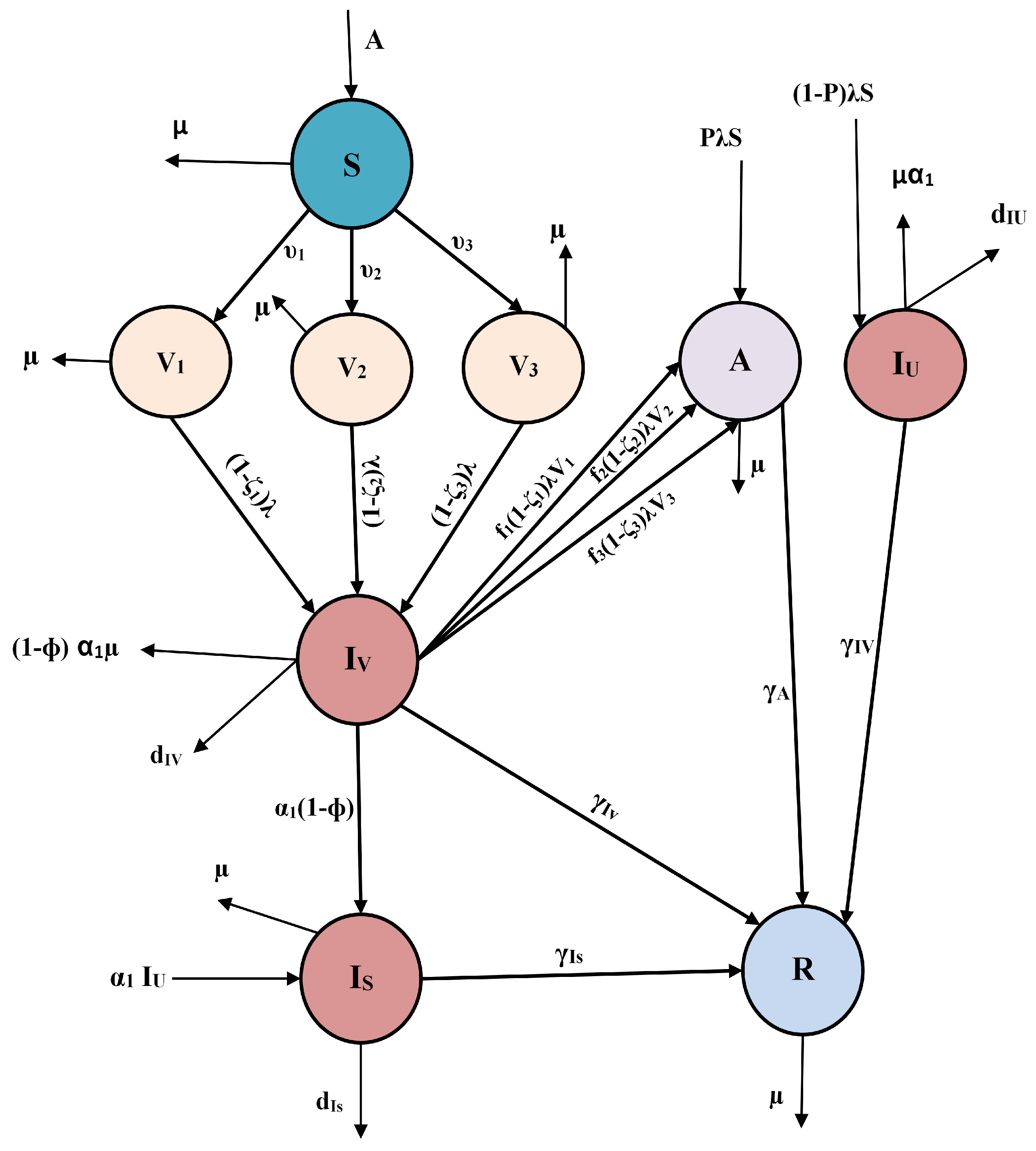
3. A Hybrid Variable-Order Mathematical Model
- 1
- 2
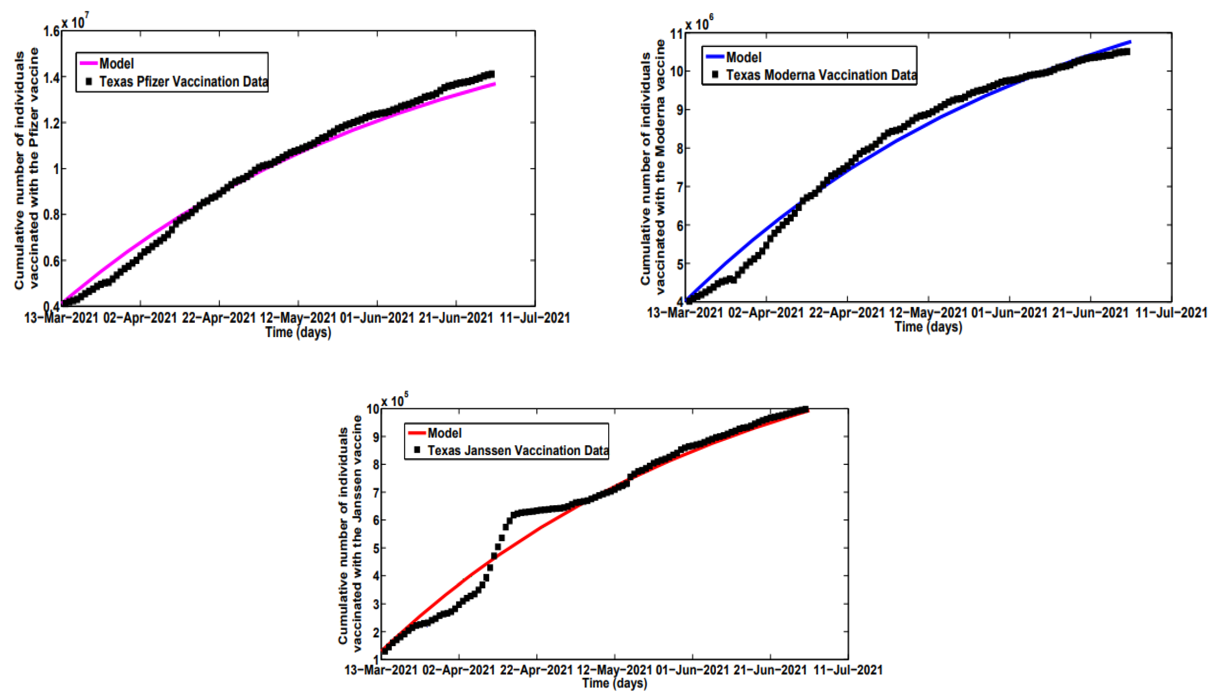
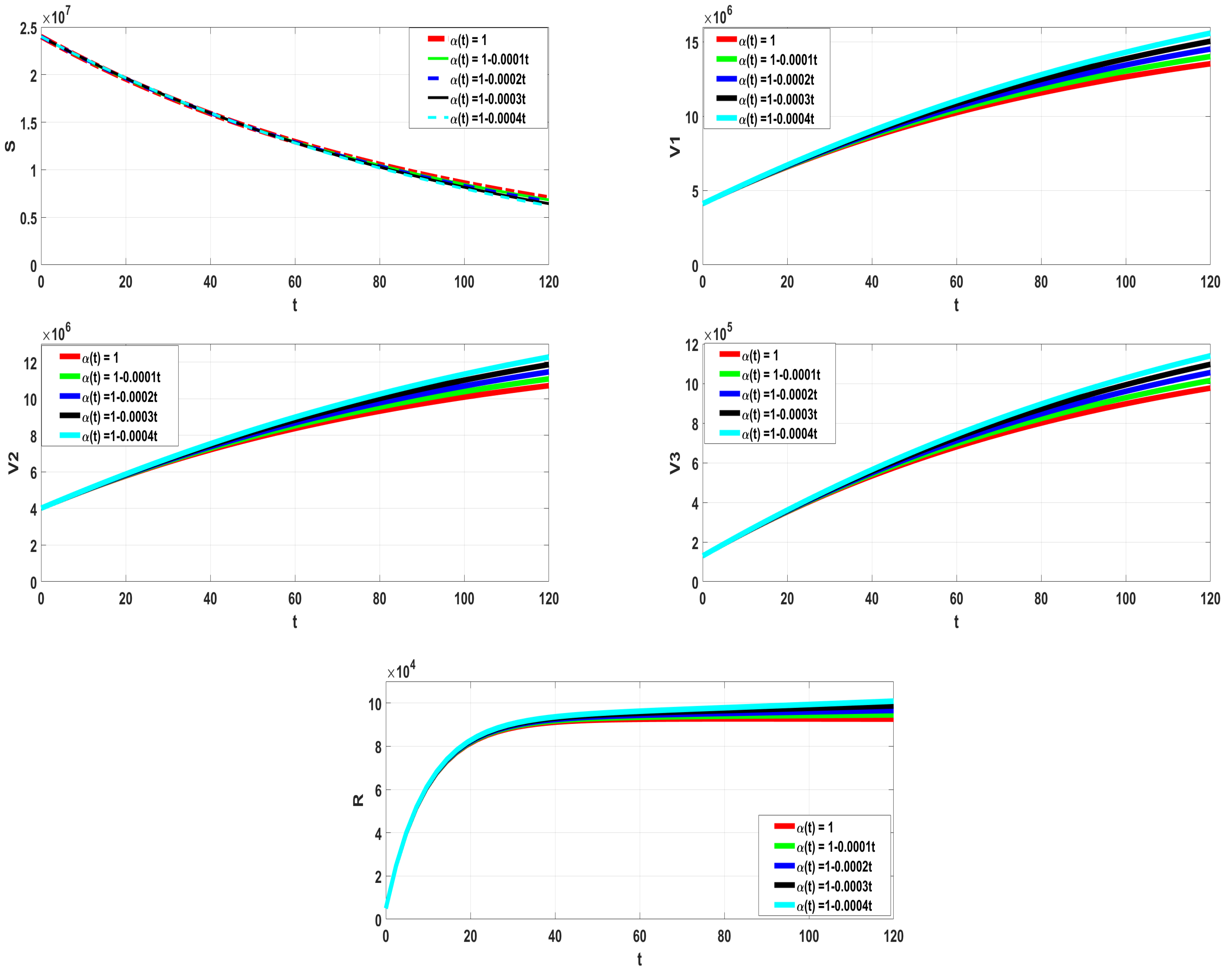
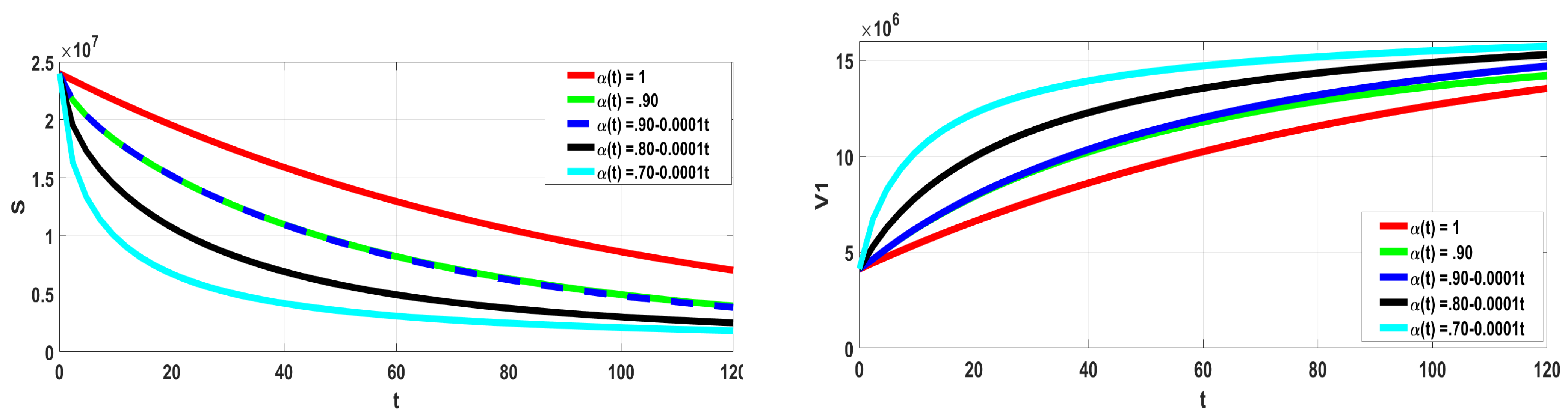
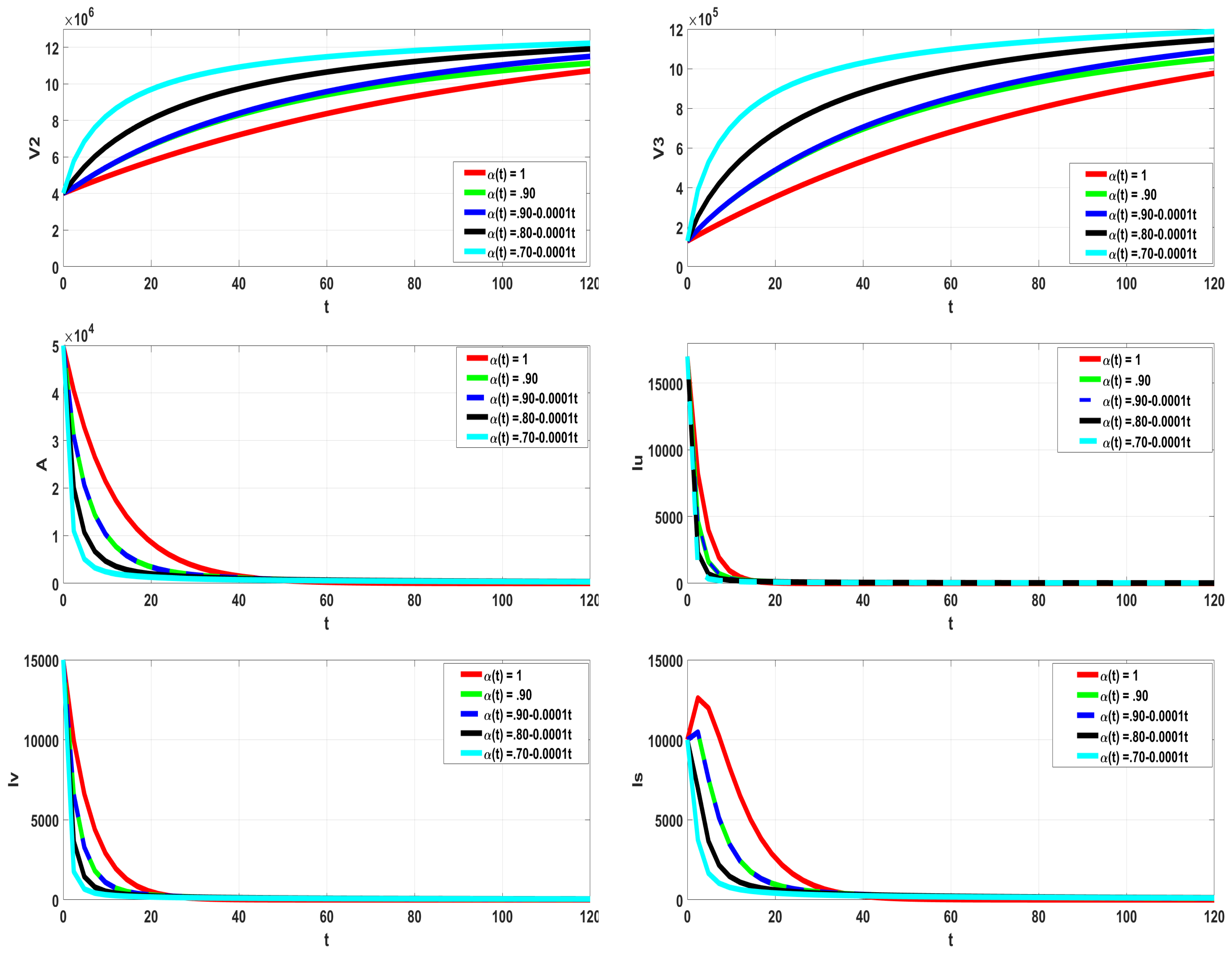
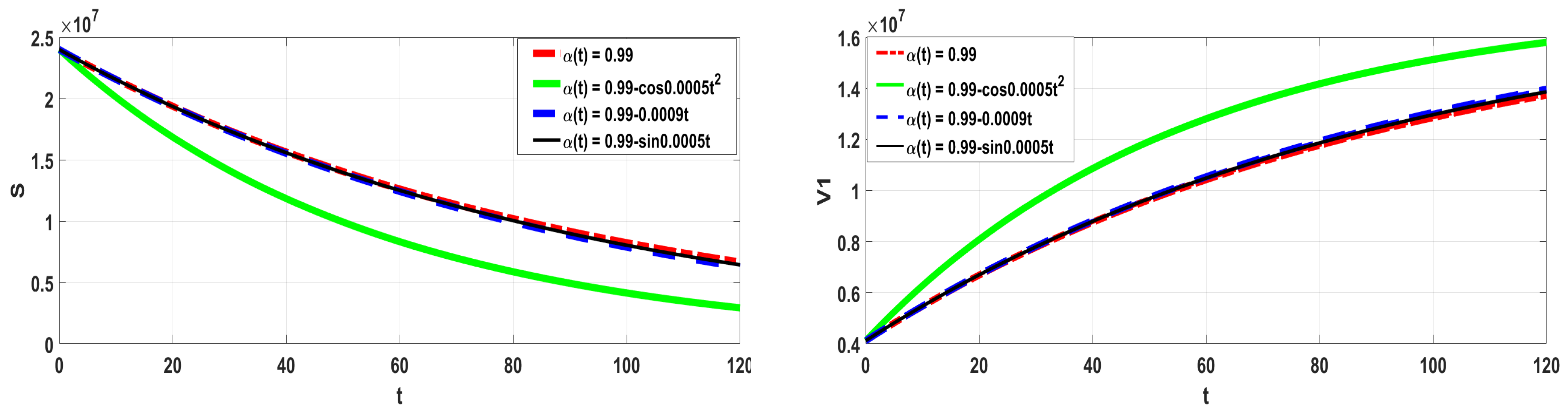
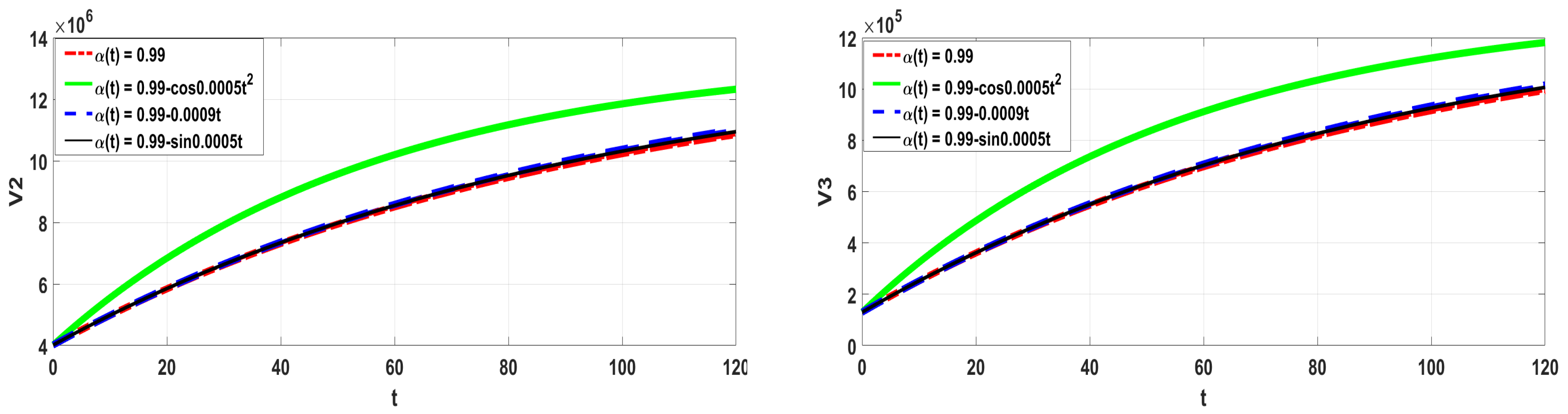
- Vaccination simulations of the proposed model in the strategy implementing only the Pfizer vaccine where these parameters are defined as in Table 2.
- 3
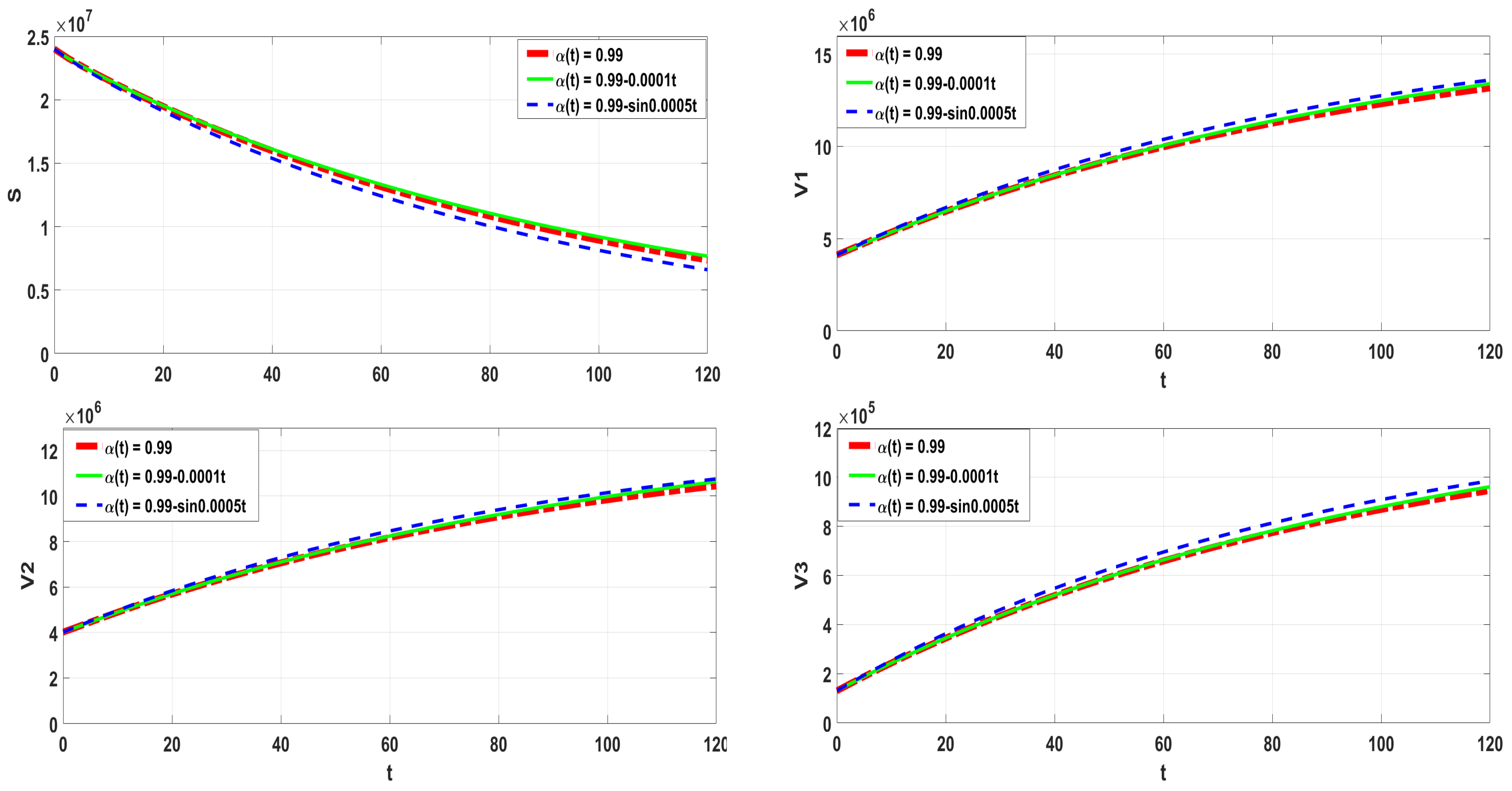
- Vaccination simulations of the proposed model in the strategy implementing only Moderna vaccine
- 4
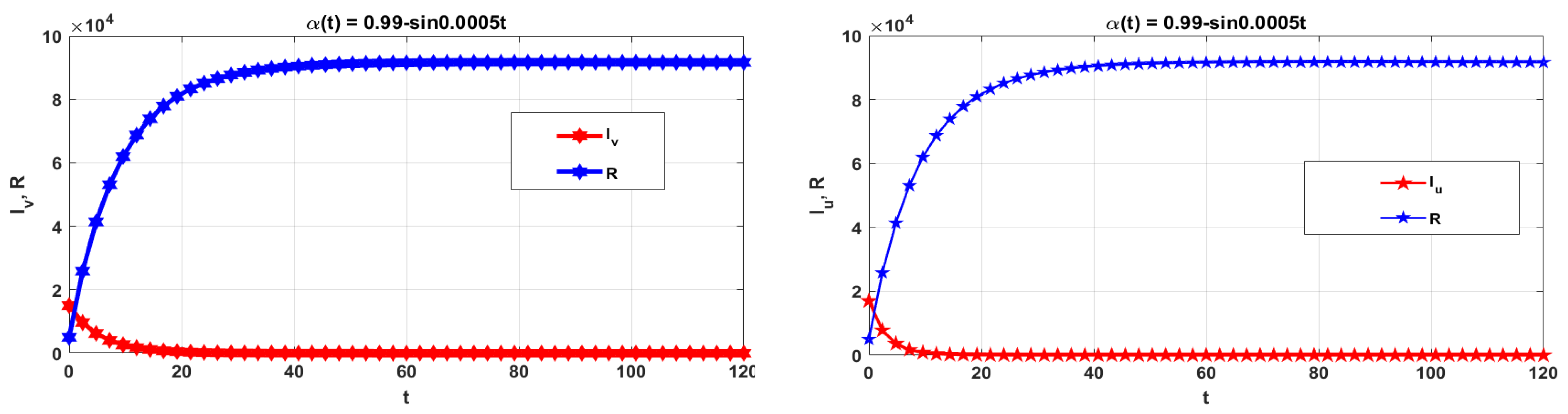
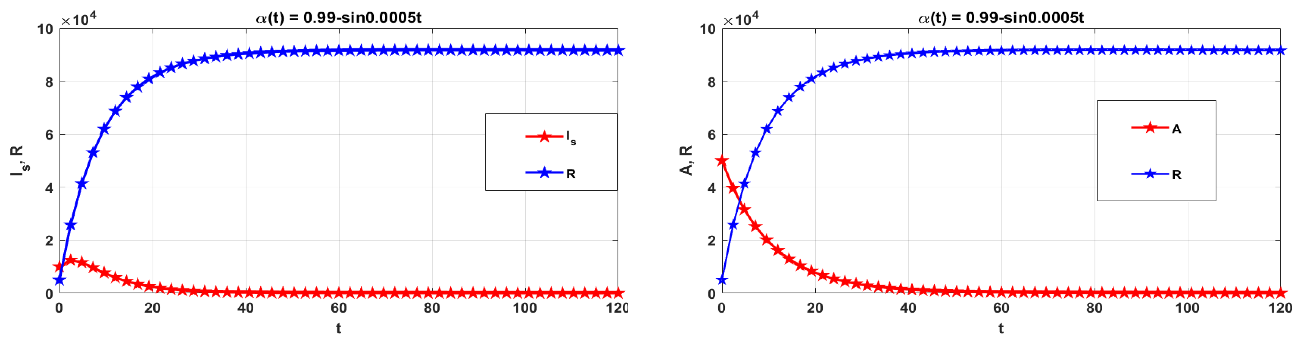
- Vaccination simulations of the proposed model in the strategy implementing only Janssen vaccine

| Variable | Interpretation |
|---|---|
| R | Humans who have recovered |
| S | Unvaccinated susceptible individuals |
| Vaccinated using vaccination number three (Oxford Johnson & Johnson) | |
| Vaccinated using vaccination number two (Moderna) | |
| Vaccinated using vaccination number one (Pfizer) | |
| Individuals with severe sickness and hospitalization who are symptomatic | |
| (vaccinated and unvaccinated) (under complete isolation) | |
| Symptomatic people who have been vaccinated | |
| Symptomatic people who have not been immunized | |
| A | Asymptomatic individuals (vaccinated and unvaccinated) |

3.1. Uniqueness and Existence
| Parameter | Interpretation | Baseline Value (per day−1) | Reference |
|---|---|---|---|
| Recruitment rate | day | [29] | |
| Rate of effective transmission | 0.00016708 | [24] | |
| Natural death rate | day | [29] | |
| Efficacy of the Janssen vaccine | [1] | ||
| Efficacy of the Moderena vaccine | [30] | ||
| Efficacy of the Pfizer vaccine | [31] | ||
| Rate of Janssen vaccination | day | [24] | |
| Rate of Moderena vaccination | day | [24] | |
| Rate of Pfizer vaccination | day | [24] | |
| p | Unvaccinated susceptibles who move to the asymptomatic stage are a small percentage of the total | [24] | |
| A parameter was changed to limit the transmissibility of asymptomatic people | [32] | ||
| Vaccine effectiveness against severe COVID-19 sickness | [2] | ||
| The percentage of susceptibles who received the vaccine and went on to develop subclinical disease | [24] | ||
| Individuals in and classes, respectively; the programme has a high rate of recovery | day | [24] | |
| Death rates from disease for people in the , and groups, respectively | [32] | ||
| The rate at which severe COVID-19 sickness develops | [32] |
3.2. Local Stability
4. Numerical Methods for Solving the Proposed Model
4.1. GRK4M
4.2. Stability of GRK4M
4.3. CPC-FDM
4.4. CPC-FDM Stability Analysis
4.5. Convergence of the Method
5. Numerical Results


6. Conclusions
Author Contributions
Funding
Data Availability Statement
Conflicts of Interest
References
- United States Food and Drug Administration. FDA Takes Key Action in Fight Against COVID-19 By Issuing Emergency Use Authorization for First COVID-19 Vaccine. 2020. Available online: https://www.fda.gov/news-events/press-announcements/fda-takes-key-action-fight-against-COVID-19-issuing-emergency-use-authorization-first-COVID-19 (accessed on 17 June 2021).
- Interim Clinical Considerations for Use of COVID-19 Vaccines Currently Authorized in the United States. Available online: https://www.cdc.gov/vaccines/COVID-19/clinical-considerations/COVID-19-vaccines-us.html (accessed on 14 July 2021).
- Machado, J.A.T.; Lope, A.M. Rare and extreme events: The case of COVID-19 pandemic. Nonlinear Dyn. 2020, 100, 2953–2972. [Google Scholar] [CrossRef] [PubMed]
- Bonyah, E.; Sagoe, A.K.; Kumar, D.; Deniz, S. Fractional optimal control dynamics of Coronavirus model with Mittag-Leffler law. Ecol. Complex. 2020, 45, 100880. [Google Scholar] [CrossRef]
- Ali, A.; Alshammari, F.S.; Islam, S.; Khan, M.A.; Ullah, S. Modeling and analysis of the dynamics of novel coronavirus (COVID-19) with Caputo fractional derivative. Results Phys. 2020, 20, 103669. [Google Scholar] [CrossRef] [PubMed]
- Danane, J.; Hammouch, Z.; Allali, K.; Rashid, S.; Singh, J. A fractional-order model ofcoronavirus disease 2019 (COVID-19) with governmental action and individual reaction. Math. Meth. Appl. Sci. 2021, 1–14. [Google Scholar] [CrossRef]
- Yadav, S.; Kumar, D.; Singh, J.; Baleanu, D. Analysis and dynamics of fractional order COVID-19 model with memory effect. Results Phys. 2021, 24, 104017. [Google Scholar] [CrossRef]
- Sinan, M.; Ali, A.; Shah, K.; Assiri, T.; Nofal, T.A. Stability analysis and optimal control of COVID-19 pandemic SEIQR fractional mathematical model with harmonic mean type incidence rate and treatment. Results Phys. 2021, 22, 103873. [Google Scholar] [CrossRef]
- Conejero, J.A.; Franceschi, J.; Picó-Marco, E. Fractional vs. Ordinary Control Systems: What Does the Fractional Derivative Provide? Mathematics 2022, 10, 2719. [Google Scholar] [CrossRef]
- Samko, S.G.; Ross, B. Integration and differentiation to a variable fractional order. Integral Transform. Spec. Funct. 1993, 1, 277–300. [Google Scholar] [CrossRef]
- Solís-Pérez, J.E.; Gómez-Aguilar, J.F. Novel numerical method for solving variable-order fractional differential equations with power, exponential and Mittag-Leffler laws. Chaos Solitons Fractals 2018, 14, 175–185. [Google Scholar] [CrossRef]
- Sun, H.; Chang, A.; Zhang, Y.; Chen, W. A review on variable-order fractional differential equations: Mathematical foundations, physical models and its applications. Fract. Calc. Appl. Anal. 2019, 22, 27–59. [Google Scholar] [CrossRef]
- Sweilam, N.H.; Al-Mekhlafi, S.M. Numerical study for multi-strain tuberculosis(TB) model of variable-order fractional derivatives. J. Adv. Res. 2016, 7, 271–283. [Google Scholar] [CrossRef]
- Sweilam, N.H.; L-Mekhlafi, S.M.A.; Shatta, S.A.; Baleanu, D. Numerical study for two types variable-order Burgers’ equations with proportional delay. Appl. Numer. Math. 2020, 156, 364–376. [Google Scholar] [CrossRef]
- Sweilam, N.H.; Assiri, T.; Hasan, M.A. Numerical solutions of nonlinear fractional Schrödinger equations using nonstandard discretizations, Numerical Solutions of Nonlinear Fractional Schrödinger Equations. Numer. Methods Partial. Differ. Equ. 2017, 33, 1399–1419. [Google Scholar] [CrossRef]
- Sweilam, N.H.; Assiri, T. Numerical scheme for solving the space-time variable order nonlinear fractional wave equation. Prog. Fract. Differ. Appl. 2015, 1, 269–280. [Google Scholar] [CrossRef]
- Bha, I.A.; Mishra, L.N. Numerical solutions of Volterra integral equations of third kind and its convergence analysis. Symmetry 2022, 14, 2600. [Google Scholar]
- Pathak, V.K.; Mishra, L.N. Application of Fixed point theorem to solvability for non-linear fractional Hadamard functional integral e quations. Mathematics 2022, 10, 2400. [Google Scholar] [CrossRef]
- Smith, G.D. Numerical solution of partial differential equations: Finite difference methods. In Oxford Applied Mathematics and Computing Science Series; Oxford University Press: Oxford, UK, 1985. [Google Scholar]
- Yuste, S.B. Weighted average finite difference methods for fractional diffusion equations. J. Comput. Phys. 2006, 216, 264–274. [Google Scholar] [CrossRef]
- Sweilam, N.H.; Hasan, M.M.A. An Improved method for nonlinear variable-order Lévy-Feller advection-dispersion equation. Bull. Malays. Math. Sci. Soc. 2019, 42, 3021–3046. [Google Scholar] [CrossRef]
- Sweilam, N.H.; Hasan, M.M.A.; Al-Mekhlafi, S.M.; Al khatib, S. Time fractional of nonlinear heat-wave propagation in a rigid thermal conductor: Numerical treatment. AEJ—Alex. Eng. J. 2022, 61, 10153–10159. [Google Scholar] [CrossRef]
- Milici, C.; Machado, J.T.; Draganescu, G. Application of the Euler and Runge–Kutta generalized methods for FDE and symbolic packages in the analysis of some fractional attractors. Int. J. Nonlinear Sci. Numer. Simul. 2020, 21, 159–170. [Google Scholar] [CrossRef]
- Omame, A.; Okuonghae, D.; Nwajeri, U.K.; Onyenegecha, C.P. A fractional-order multi-vaccination model for COVID-19 with non-singular kernel. Alex. Eng. J. 2022, 16, 6089–6104. [Google Scholar] [CrossRef]
- Sun, H.G.; Chen, W.; Wei, H.; Chen, Y.Q. A comparative study of constant-order and variable-order fractional models in characterizing memory property of systems. Eur. Phys. J. Spec. Top. 2011, 193, 185–192. [Google Scholar] [CrossRef]
- Baleanu, D.; Fernandez, A.; Akgül, A. On a fractional operator combining proportional and classical differintegrals. Mathematics 2020, 8, 360. [Google Scholar] [CrossRef]
- Ullah, M.Z.; Baleanu, D. A new fractional SICA model and numerical method for the transmission of HIV/AIDS. Math. Meth. Appl. Sci. 2021, 44, 4648–4659. [Google Scholar] [CrossRef]
- Lin, W. Global existence theory and chaos control of fractional differential equations. J. Math. Anal. Appl. 2007, 332, 709–726. [Google Scholar] [CrossRef]
- Texas Population, Census Reporter. Available online: https://censusreporter.org/profiles/04000US48-texas/ (accessed on 26 June 2021).
- United States Food and Drug Administration. FDA Briefing Document Moderna COVID-19 Vaccine. 2020. Available online: https://www.fda.gov/media/144434/download (accessed on 17 June 2021).
- United States Food and Drug Administration. FDA Briefing Document Pfizer-BioNTech COVID-19 Vaccine. 2020. Available online: https://www.fda.gov/media/144245/download (accessed on 17 June 2021).
- Okuonghae, D.; Omame, A. Analysis of a mathematical model for COVID-19 population dynamics in Lagos, Nigeria. Chaos Solitons Fractals 2020, 139, 110032. [Google Scholar] [CrossRef]
- Chu, Y.-M.; Yassen, M.F.; Ahmad, I.; Sunthrayuth, P.; Khan, M.A. A fractional SARS-COV-2 model with Atangana-Baleanu derivative: Application to fourth wave. Fractals 2022, 30, 2240210. [Google Scholar] [CrossRef]
- Driessche, P.; Watmough, P. Reproduction numbers and sub-threshold endemic equilibria for compartmental models of disease transmission. Math. Biosci. 2002, 180, 29–48. [Google Scholar] [CrossRef]
- Fosu, G.O.; Akweittey, E. Albert-adu-sackey, Next-generation matrices and basic reproductive numbers for all phases of the Coronavirus disease. Open J. Math. Sci. 2020, 4, 261–272. [Google Scholar] [CrossRef]
- Sekerci, Y. Climate change forces plankton species to move to get rid of extinction: Mathematical modeling approach. Eur. Phys. J. Plus 2020, 135, 794. [Google Scholar] [CrossRef]
- Al-Mekhlafi, S.M.; Sweilam, N.H. Numerical Studies for Some Tuberculosis Models; LAP LAMBERT Academic Publishing: London, UK, 2016; 156p. [Google Scholar]
- Sweilam, N.H.; L-Mekhlafi, S.M.A.; Alshomrani, A.S.; Baleanu, D. Comparative study for optimal control nonlinear variable-order fractional tumor model. Chaos Solitons Fractals 2020, 136, 109810. [Google Scholar] [CrossRef]
- Scherer, R.; Kalla, S.; Tang, Y.; Huang, J. The Grünwald-Letnikov method for fractional differential equations. Comput. Math. Appl. 2011, 62, 902–917. [Google Scholar] [CrossRef]
- Arenas, A.J.; Gonzàlez-Parra, G.; Chen-Charpentierc, B.M. Construction of nonstandard finite difference schemes for the SI and SIR epidemic models of fractional order. Math. Comput. Simul. 2016, 121, 48–63. [Google Scholar] [CrossRef]
- Yuste, S.B.; Quintana-Murillo, J. A finite difference method with non-uniform time steps for fractional diffusion equations. Comput. Phys. Commun. 2012, 183, 2594–2600. [Google Scholar] [CrossRef]
- COVID-19 Vaccinations in the US. Available online: https://data.cdc.gov/Vaccinations/COVID-19-Vaccinations-in-the-United-States-Jurisdi/uns (accessed on 13 March 2021).
Disclaimer/Publisher’s Note: The statements, opinions and data contained in all publications are solely those of the individual author(s) and contributor(s) and not of MDPI and/or the editor(s). MDPI and/or the editor(s) disclaim responsibility for any injury to people or property resulting from any ideas, methods, instructions or products referred to in the content. |
© 2023 by the authors. Licensee MDPI, Basel, Switzerland. This article is an open access article distributed under the terms and conditions of the Creative Commons Attribution (CC BY) license (https://creativecommons.org/licenses/by/4.0/).
Share and Cite
Sweilam, N.; Al-Mekhlafi, S.M.; Salama, R.G.; Assiri, T.A. Numerical Simulation for a Hybrid Variable-Order Multi-Vaccination COVID-19 Mathematical Model. Symmetry 2023, 15, 869. https://doi.org/10.3390/sym15040869
Sweilam N, Al-Mekhlafi SM, Salama RG, Assiri TA. Numerical Simulation for a Hybrid Variable-Order Multi-Vaccination COVID-19 Mathematical Model. Symmetry. 2023; 15(4):869. https://doi.org/10.3390/sym15040869
Chicago/Turabian StyleSweilam, Nasser, Seham M. Al-Mekhlafi, Reem G. Salama, and Tagreed A. Assiri. 2023. "Numerical Simulation for a Hybrid Variable-Order Multi-Vaccination COVID-19 Mathematical Model" Symmetry 15, no. 4: 869. https://doi.org/10.3390/sym15040869