Exact (1 + 3 + 6)-Dimensional Cosmological-Type Solutions in Gravitational Model with Yang–Mills Field, Gauss–Bonnet Term and Λ Term

Abstract

We consider a 10-dimensional gravitational model with an SO(6)Yang–Mills field, Gauss–Bonnet term, and $\Lambda$ term. We study so-called cosmological-type solutions defined on the product manifold $M=\mathbb{R}\times {\mathbb{R}}^3\times K$, where K is $6d$ a Calabi–Yau manifold. By setting the gauge field 1-form to coincide with the 1-form spin connection on K, we obtain exact cosmological solutions with exponential dependence of scale factors (upon t-variable) governed by two non-coinciding Hubble-like parameters: $H>0$ and h obeying $H+2h\ne 0$. We also present static analogs of these cosmological solutions (for $H\ne 0$, $h\ne H$, and $H+2h\ne 0$). The islands of stability for both classes of solutions are outlined.

1. Introduction

Here we deal with a so-called Einstein–Gauss–Bonnet–Yang–Mills–$\Lambda$ gravitational model in dimension $D=10$. The action of the model contains scalar curvature, a Gauss–Bonnet term, a cosmological term ($\Lambda$ term), and a Yang–Mills term with a value in $so\left(6\right)$ Lie algebra. The model includes a non-zero constant $\alpha$, coupled to the sum of the Yang–Mills and Gauss–Bonnet terms. The equations of motion for this model are of second order (as it takes place in general relativity). The so-called Gauss–Bonnet term has appeared in (super)string theory as a second-order correction in curvature to the effective (super)string effective action [1,2,3] for a heterotic string [4].

At present, Einstein–Gauss–Bonnet (EGB) gravitational models, e.g., with a cosmological term and extra matter fields, and their modifications [5,6,7,8,9,10,11,12,13,14,15,16,17,18,19,20,21,22,23,24,25,26], are under intensive study in astrophysics and cosmology. The main goal in these studies is a solution to the dark energy problem. One can study such models for a possible explanation of the accelerating expansion of the Universe, which was supported by supernovae (type Ia) observational data [27,28].

We note that, at present, there exist several modifications of Einstein and EGB actions which correspond to $F\left(R\right)$, $R+f\left(\mathcal{G}\right)$, $f\left(R,\mathcal{G}\right)$, $f\left(R,\mathcal{G}\right)$, $f(R,\mathcal{G},T_{..}{T}^{..})$ theories (e.g., for $D=4$), where R is the scalar curvature and $\mathcal{G}$ is the Gauss–Bonnet term. These modifications are under intensive studying devoted to cosmological, astrophysical, and other applications; see [29,30,31,32,33,34,35] and references therein.

Another point of interest is the search for possible local manifestations of dark energy related to wormholes, black holes, etc. The most important results for black holes in models with Gauss–Bonnet terms are related to the Boulware–Deser–Wheeler solution [36,37] and its generalizations [38,39,40,41]; see also Refs. [42,43,44] and references therein. For certain applications of brane-world models with Gauss–Bonnet term, see Refs. [45,46] and related bibliography. For wormhole solutions in Einstein–Gauss–Bonnet models with certain fields, see Refs. [47,48] and references therein.

In this article, we deal with the so-called cosmological-type solutions with the $10d$ metric

$$g^{\left(10\right)}=-wd\chi \otimes d\chi +a_3^2\left(\chi \right)g^{\left(3\right)}+a_6^2\left(\chi \right)g^{\left(6\right)}.$$

(1)

defined on a product manifold $\mathbb{R}\times {\mathbb{R}}^3\times K,$ where $w=\pm 1$, ${\mathbb{R}}^3$ is a flat $3d$ manifold (“our” space) with the metric $g^{\left(3\right)}$, and K is a $6d$ Ricci-flat Calabi–Yau manifold (internal space) of an $SU\left(3\right)$ holonomy group with the metric $g^{\left(6\right)}$. The warped product model is governed by two scale factors depending upon one variable $\chi$. It is the synchronous time variable for the cosmological case $w=1$: $\chi =t$, while it coincides with the space-like variable for $w=-1$: $\chi =u$. The presence of a Yang–Mills field makes this ansatz consistent if we choose the Lie algebra for the Yang–Mills field to be equal (at least) to $so\left(6\right)$, which contains $su\left(3\right)$ subalgebra, corresponding to an $SU\left(3\right)$ group of golonomy of the $6d$ Calabi–Yau manifold. For the Yang–Mills field, we consider the following ansatz: we put here the gauge field 1-form to be equal to the spin connection 1-form on K (see Section 2): $A={\omega }^{\left(6\right)}$. In such an ansatz, the gauge field plays the role of compensator, which “waves out” the terms with non-zero Riemann tensors of the Calabi–Yau metric $g^{\left(6\right)}$.

Originally, such an idea of compensation was used by Wu and Wang [49] (see also [50]) in a $(1+3+6)$-dimensional cosmological model based on $10d$ Yang=-Mills ($SO\left(32\right)$- and/or $E_8\times E_8$-) supergravity theory “upgrated” by additions of Chern–Simons and Gauss–Bonnet terms (of superstring origin). The work of Wu and Wang was influenced greatly by the well-known paper of Candelas et al. [51], devoted to vacuum configurations in ten-dimensional $O\left(32\right)$ and $E_8\times E_8$ supergravity and superstring theory that have unbroken $N=1$ supersymmetry in four dimensions.

It should be noted that compactifications of 11-dimensional supergravity on a ($6d$) Calabi–Yau manifold were considered in Refs. [52,53]. Moreover, $4d$ and $6d$ Calabi–Yau manifolds also appeared in partially sypersymmetric solutions of $D=11$ supergravity with M-branes; see Refs. [54,55,56] and and references threin.

In Section 3 we obtain exact cosmological solutions with exponential dependence of scale factors (upon the t-variable) governed by two non-coinciding Hubble-like parameters: $H>0$ and h, corresponding to factor spaces of dimensions 3 and 6, respectively, when the following restriction $3H+6h\ne 0$ is used (excluding the solutions with a constant volume factor).

In Section 4, we obtain static solutions ($w=-1$) for non-coinciding Hubble parameters $H\ne 0$, h, which obey $3H+6h\ne 0$. We also study the stability (in a certain restricted sense) of the obtained solutions in the cosmological case for $t\to +\infty$ (see Section 3) and in the static case for $u\to \pm \infty$ (see Section 4) by using the results of Ref. [22] (see also the approach of Ref. [19]) and single out the subclasses of stable/non-stable solutions.

2. The 10-Dimensional Model

2.1. The Action and Equations of Motion

We take the action of the model as

$$\begin{array}{c}\hfill S=\frac{1}{2{\kappa }^2}\int d^{10}x\sqrt{-g}\left\{R+\alpha \left[\mathrm{tr}{F}_{MN}{F}^{MN}\right.\right.\\ \hfill \left.\left.+R_{MNPQ}{R}^{MNPQ}-4R_{MN}{R}^{MN}+R^2\right]\right\},\end{array}$$

(2)

where ${\kappa }^2$ is the 10-dimensional gravitational constant, $\alpha \ne 0$ is a constant, $g_{MN}$ are components of the metric, and $F_{MN}$ are components of the Yang–Mills field strengths corresponding to the 2-form with the value in the Lie algebrs $so\left(6\right)$: $F=\frac{1}{2}{F}_{MN}d{x}^M\wedge d{x}^N=dA+A\wedge A,$ where $A=A_{M}d{x}^M$ is the 1-form with the value in $so\left(6\right)$ ($F_{MN}={\partial }_M{A}_N-{\partial }_N{A}_M+[A_M,A_N]$).

The action (2) leads us to the following equations of motions:

$$\begin{array}{c}\hfill R_{MN}-\frac{1}{2}{g}_{MN}R=-2\alpha \left(\mathrm{tr}{F}_{MP}{F}_N^P-\frac{1}{4}{g}_{MN}\mathrm{tr}{F}_{PQ}{F}^{PQ}\right)\\ \hfill +\alpha [\frac{1}{2}{g}_{MN}(R_{MNPQ}{R}^{MNPQ}-4R_{MN}{R}^{MN}+R^2)-2R{R}_{MN}\\ \hfill +4R_{MP}{R}_N^P+4R_{MPNQ}{R}^{PQ}-2R_M^{PQS}{R}_{NPQS}],\end{array}$$

(3)

$$D_M{F}^{MP}=0.$$

(4)

Here, we use the following notation for the covariant gauge derivative: $D_M=D_M\left(A\right)={\nabla }_M+[A_M,.]$.

2.2. Cosmological Ansatz

Let us consider a ten-dimensional manifold

$$M=\mathbb{R}\times {\mathbb{R}}^3\times K,$$

(5)

where K is a $6d$ Calabi–Yau manifold, i.e., a compact 6-dimensional Kähler Ricci-flat manifold with the metric, which has an $SU\left(3\right)$ holonomy group. For the corresponding Lie algebra, we have $su\left(3\right)\subset so\left(6\right)$.

We start with the cosmological case, i.e., we consider the set of Equations (3) and (4) on the manifold (5) with the following ansatz for fields:

$$\begin{array}{c}\hfill g^{\left(10\right)}=-dt\otimes dt+a_3^2\left(t\right)g^{\left(3\right)}+a_6^2\left(t\right)g^{\left(6\right)},\end{array}$$

(6)

$${\displaystyle \begin{array}{c}\hfill A={\omega }^{\left(6\right)}.\end{array}}$$

(7)

Here, $g^{\left(3\right)}=d{x}^1\otimes d{x}^1+d{x}^2\otimes d{x}^2+d{x}^3\otimes d{x}^3$, i.e., we deal with a flat Euclidean metric on ${\mathbb{R}}^3$, and $g^{\left(6\right)}=g_{mn}^{\left(6\right)}\left(y\right)d{y}^m\otimes d{y}^n$ is the Calabi–Yau metric on K.

By ${\omega }^{\left(6\right)}={\omega }_m^{\left(6\right)}\left(y\right)d{y}^m$, we denote the spin connection 1-form on K with the value in the Lie algebra $so\left(6\right)$ (in fact, it belongs to subalgebra $su\left(3\right)\subset so\left(6\right)$) corresponding to the (local) basis of co-vectors $e_m^a$ on K, which diagonalizes the metric $g^{\left(6\right)}$:

$$g_{mn}^{\left(6\right)}=e_m^a{e}_n^b{\delta }_{ab},$$

(8)

$${\omega }_m^{\left(6\right)}=\mid \mid {\omega }_{bm}^{\left(6\right)a}\mid \mid \equiv \mid \mid e_n^a{\nabla }_m^{\left(6\right)}{e}_b^n\mid \mid \subset so\left(6\right),$$

(9)

where the covariant derivative ${\nabla }_m^{\left(6\right)}$ corresponds to the metric $g^{\left(6\right)}$, and $e_b^n$ is the “inverse” (dual) basis of vector fields obeying $e_n^a{e}_b^n={\delta }_b^a$.

It follows from (7) that

$$F={\mathrm{\Omega }}^{\left(6\right)},$$

(10)

where ${\mathrm{\Omega }}^{\left(6\right)}=d{\omega }^{\left(6\right)}+{\omega }^{\left(6\right)}\wedge {\omega }^{\left(6\right)}$ is the curvature two-form on K with the value in $so\left(6\right)$.

The spin connection ${\omega }^{\left(6\right)}$ on K obeys the identity

$$D_m\left({\omega }^{\left(6\right)}\right){\mathrm{\Omega }}^{\left(6\right)mn}=0,$$

(11)

where $D_m\left({\omega }^{\left(6\right)}\right)={\nabla }_m^{\left(6\right)}+[{\omega }_m^{\left(6\right)},.]$. identity (11) is equivalent to the following identity for the Riemann tensor on K:

$${\nabla }_m^{\left(6\right)}{R}^{\left(6\right)mnpq}=0,$$

(12)

which is valid for any Kähler–Ricci-flat manifold [57].

The Yang–Mills Equation (4) is satisfied identically due to Equations (6), (7), and (11).

Let us denote

$$H\left(t\right)\equiv {\dot{a}}_3/a_3,h\left(t\right)\equiv {\dot{a}}_6/a_6,$$

(13)

where in this section we denote $\dot{a}\equiv \frac{da}{dt}$.

Then, Equation (3) for the ansatz (6) and (7) may be written as follows:

$$\begin{array}{c}\hfill B_0+2\Lambda -\alpha B_1=0,\end{array}$$

(14)

$$\begin{array}{c}\hfill \frac{d{L}_H}{dt}+(3H+6h)L_H-L_0=0,\end{array}$$

(15)

$$\begin{array}{c}\hfill \frac{d{L}_h}{dt}+(3H+6h)L_h-L_0=0.\end{array}$$

(16)

Here

$$\begin{array}{c}\hfill L_0=B_0-2\Lambda -\frac{1}{3}\alpha B_1,\end{array}$$

(17)

$$\begin{array}{c}\hfill L_H=2B_H-\frac{4}{3}\alpha A_H,\end{array}$$

(18)

$$\begin{array}{c}\hfill L_h=2B_h-\frac{4}{3}\alpha A_h,\end{array}$$

(19)

$$\begin{array}{c}\hfill B_0=3H^2+6h^2-{(3H+6h)}^2,\end{array}$$

(20)

$$\begin{array}{c}\hfill B_H=H-(3H+6h),\end{array}$$

(21)

$$\begin{array}{c}\hfill B_h=h-(3H+6h),\end{array}$$

(22)

$$\begin{array}{c}\hfill B_1=144H^{3}h+1080H^2{h}^2+1440H{h}^3+360h^4\end{array}$$

(23)

and

$$\begin{array}{c}\hfill A_H=36H^{2}h+180H{h}^2+120h^3,\end{array}$$

(24)

$$\begin{array}{c}\hfill A_h=6H^3+90H^{2}h+180H{h}^2+60h^3.\end{array}$$

(25)

Equations (14)–(16) are obtained from (3) using the Ricci flatness of K and the equality for the Riemann tensor of the internal space K with the metric $g^{\left(6\right)}$

$$R_{pqmn}^{\left(6\right)}{R}^{\left(6\right)q{p}^{\prime }mn}=g^{\left(6\right)m{p}^{\prime }}{g}^{\left(6\right)nq}\mathrm{tr}{F}_{mn}{F}_{pq},$$

(26)

which follows from (10) and the well-known identity

$$R_{qmn}^{\left(6\right)p}=e_a^p{e}_q^b{\mathrm{\Omega }}_{bmn}^{\left(6\right)a}.$$

(27)

3. Cosmological Solutions

Here, we consider the case when Hubble-like parameters are constant, i.e.,

$$H\left(t\right)=H=\mathrm{const},h\left(t\right)=h=\mathrm{const}.$$

(28)

For scale factors, we obtain an exponential dependence on t

$$a_3\left(t\right)=exp\left(Ht\right),a_6\left(t\right)=exp\left(ht\right).$$

(29)

We obtain a set of polynomial equations

$$\begin{array}{c}\hfill B_0+2\Lambda -\alpha B_1=0,\end{array}$$

(30)

$$\begin{array}{c}\hfill (3H+6h)L_H-L_0=0,\end{array}$$

(31)

$$\begin{array}{c}\hfill (3H+6h)L_h-L_0=0,\end{array}$$

(32)

where the polynomials $B_0,B_1,L_0,L_H,$ and $L_h$ are defined above.

We set

$$H>0.$$

(33)

This relationship is used for a description of an accelerated expansion of the 3-dimensional subspace (which may describe our Universe). The evolution of the 6-dimensional internal factor space is described by the Hubble-like parameter h.

It follows from Refs. [22,24] (for a more general splitting scheme, see the paper by Chirkov, Pavluchenko, and Toporensky [18]) that if we consider Hubble-like parameters H and h obeying the two restrictions imposed,

$$3H+6h\ne 0,H\ne h,$$

(34)

we reduce the relationships (30)–(32) to the following set of equations:

$$\begin{array}{c}\hfill E=3H^2+6h^2-{(3H+6h)}^2+2\Lambda \\ \hfill -\alpha [144H^{3}h+1080H^2{h}^2+1440H{h}^3+360h^4]=0,\end{array}$$

(35)

$$Q=2H^2+20Hh+20h^2=-\frac{1}{2\alpha }.$$

(36)

Using Equation (36), we obtain

$$H={(-2\alpha \mathcal{P})}^{-1/2},$$

(37)

where

$$\begin{array}{c}\hfill \mathcal{P}=\mathcal{P}\left(x\right)\equiv 2+20x+20x^2,\end{array}$$

(38)

$$\begin{array}{c}\hfill x\equiv h/H,\end{array}$$

(39)

and

$$\alpha \mathcal{P}<0.$$

(40)

Due to restrictions (34), we have for x from (39)

$$x\ne x_d\equiv -1/2,x\ne x_a\equiv 1.$$

(41)

The relationship (36) is valid only if

$$\mathcal{P}\left(x\right)\ne 0.$$

(42)

Substituting relationship (37) into (35), we obtain

$$\begin{array}{c}\hfill \Lambda \alpha \equiv \lambda =f\left(x\right)\equiv (1/4)[3+6x^2-{(3+6x)}^2]{(2+20x+20x^2)}^{-1}\\ \hfill +(1/8)\left[18(8x+60x^2+80x^3+20x^4)\right]{(2+20x+20x^2)}^{-2}.\end{array}$$

(43)

From (42), we obtain

$$x\ne x_{\pm }\equiv \frac{-10\pm \sqrt{10}}{20},$$

(44)

where $x_{\pm }$ are roots of the quadratic equation $\mathcal{P}\left(x\right)=0$. They obey

$$x_{-}<x_{+}<0.$$

(45)

According to Equation (40), we obtain (in this cosmological case)

$$x_{-}<x<x_{+}\mathrm{for}\alpha >0,$$

(46)

and

$$x<x_{-}\mathrm{or}x>x_{+}\mathrm{for}\alpha <0.$$

(47)

The graphical representation of the function $\lambda =f\left(x\right)$ is given in Figure 1.

The function $f\left(x\right)$ obeys

$$\underset{x\to \pm \infty }{lim}f\left(x\right)={\lambda }_{\infty }\equiv -\frac{21}{80}$$

(48)

and

$$\underset{x\to x_{\pm }}{lim}f\left(x\right)=-\infty .$$

(49)

It has a maximum at $x_c=-\frac{1}{5}$ with the value $f\left(x_c\right)={\lambda }_c\equiv 3/10$ and an inflection point at $x_d=-\frac{1}{2}$ with the value $f\left(x_d\right)={\lambda }_d\equiv 3/16$. It has also a point of local maximum at $x_a\equiv 1$ with the value $f\left(x_a\right)={\lambda }_a\equiv -3/14$.

Equation (43) is equivalent to the following master equation:

$$(400\lambda +105)x^4+(800\lambda +150)x^3+(480\lambda +90)x^2+(80\lambda +30)x+4\lambda +3=0.$$

(50)

For

$$\lambda \ne {\lambda }_{\infty }\equiv -21/80$$

(51)

the solution to this (fourth order) master equation reads

$$\begin{array}{c}\hfill x={\epsilon }_1\frac{1}{2}\sqrt{-\frac{{\epsilon }_{2}A}{\sqrt{X}}-Y^{1/3}+B{Y}^{-1/3}+C}\\ \hfill -{\epsilon }_2\frac{\sqrt{X}}{2\sqrt{5}(80\lambda +21)}-\frac{5(16\lambda +3)}{2(80\lambda +21)},\end{array}$$

(52)

where ${\epsilon }_1=\pm 1$, ${\epsilon }_2=\pm 1$,

$$\begin{array}{c}\hfill A=\left(18\sqrt{5}(1280{\lambda }^2+96\lambda -39)\right)/{(80\lambda +21)}^2,\end{array}$$

(53)

$$\begin{array}{c}\hfill B=-\left(4(16\lambda -3)(20\lambda +3)\right)/(5{(80\lambda +21)}^2),\end{array}$$

(54)

$$\begin{array}{c}\hfill C=\left(2(16\lambda +3)(80\lambda -9)\right)/{(80\lambda +21)}^2,\end{array}$$

(55)

and

$$\begin{array}{c}\hfill X=5{(80\lambda +21)}^2{Y}^{1/3}+5(16\lambda +3)(80\lambda -9)+4(16\lambda -3)(20\lambda +3)Y^{-1/3},\end{array}$$

(56)

$$\begin{array}{c}\hfill Y=(36(16\lambda -3)\sqrt{-(10\lambda -3)(14\lambda +3)})/(5^{3/2}{(80\lambda +21)}^3)+Z,\end{array}$$

(57)

$$\begin{array}{c}\hfill Z=\left(4(16\lambda -3)(320{\lambda }^2+42\lambda -9)\right)/(5{(80\lambda +21)}^3).\end{array}$$

(58)

It follows from Figure 1 that for the given parameters $\Lambda$ and $\alpha$, obeying restrictions $\alpha \ne 0$ and (51), real solutions in formula (52) appear for suitably chosen ${\epsilon }_1=\pm 1$ and ${\epsilon }_2=\pm 1$ if

$$\lambda =\Lambda \alpha \le {\lambda }_c=3/10$$

(59)

for $\alpha >0$ and

$$\lambda =\Lambda \alpha <{\lambda }_a=-3/14$$

(60)

for $\alpha <0$.

For example, the $\lambda ={\lambda }_c=3/10$ relationship (52) gives us $x=x_c=-1/5$ if we put ${\epsilon }_1=\pm 1$ and ${\epsilon }_2=-1$.

In exceptional cases,

$$\lambda ={\lambda }_{\infty }=-21/80$$

(61)

we have a cubic master Equation (50) which has three real roots,

$$x=x_k=(1/10)(-2-6cos(\theta /3+2k\pi /3)),tan\theta =\sqrt{15},$$

(62)

$k=1,2,3$, or, numerically

$$x_1\approx 0.29253505115,x_2\approx -0.14952367803,x_3\approx -0.74301143583.$$

(63)

Graphical analysis. The graphical representation $\Lambda \left|\alpha \right|$ upon $x=h/H$ (in this cosmological case) is presented in Figure 2. In drawing this figure, we use the relationship

$$\Lambda \left|\alpha \right|=\lambda \mathrm{sgn}\left(\alpha \right)=f\left(x\right)\frac{(-2-20x-20x^2)}{|2+20x+20x^2|},$$

(64)

in agreement with (38) and (40). It follows from Figure 2 that real solutions take place if

$$\Lambda \left|\alpha \right|\le {\lambda }_c=3/10,$$

(65)

for $\alpha >0$ and

$$\Lambda \left|\alpha \right|>|{\lambda }_a|=3/14,$$

(66)

for $\alpha <0$. (The point $x_a=1$ is excluded from our consideration.)

Stability. Using the results of Refs. [22,24], we obtain that the cosmological solutions under consideration obeying $x=h/H\ne x_i$, $i=a,c,d$, where $x_a=1$, $x_c=-\frac{1}{5}$, $x_d=-\frac{1}{2}$, are stable if (i) $x>x_d=-1/2$ and unstable if (ii) $x<x_d=-1/2$. (For isotropic cosmological solutions with $H=h$, see Refs. [17,22] for generic $\Lambda$ and [14,15] for $\Lambda =0$).

We note that the the points $x_a=1$ and $x_d=-1/2$ are excluded from our consideration due to restrictions (34), while the point of maximum $x_c=-\frac{1}{5}$ is excluded since the analysis of Ref. [22] was based on the equations for perturbations for $\delta H\left(t\right)$, $\delta h\left(t\right)$ in the linear approximation, which can be resolved when $x_c\ne -\frac{1}{5}$. In the special case $x_c=-\frac{1}{5}$, higher-order terms in pertubations should be considered.

Let us denote by $n_s$ the number of non-special stable solutions. By using Figure 2, we find just graphically for $\alpha >0$

$$n_s=\left\{\begin{array}{c}0,\Lambda \alpha \ge {\lambda }_c=3/10,\hfill \\ 2,{\lambda }_d=3/16<\Lambda \alpha <{\lambda }_c=3/10,\hfill \\ 1,\Lambda \alpha \le {\lambda }_d=3/16.\hfill \end{array}\right.$$

(67)

(here ${\lambda }_i=f\left(x_i\right)$), while for $\alpha <0$, we obtain

$$n_s=\left\{\begin{array}{c}1,\Lambda \left|\alpha \right|\ge |{\lambda }_{\infty }|=21/80,\hfill \\ 2,|{\lambda }_a|=3/14<\Lambda |\alpha |<|{\lambda }_{\infty }|=21/80,\hfill \\ 0,\Lambda \left|\alpha \right|\le |{\lambda }_a|=3/14.\hfill \end{array}\right.$$

(68)

Thus, for $\alpha >0$ and a small enough value of $\Lambda$, there exists at least one stable solution with $x\in (x_{-},x_{+})$, while for $\alpha <0$ and a big enough value of $\Lambda$, there exists at least one stable solution with x obeying $x>x_{+}$. The solutions with $x<x_{-}$ are unstable.

In the cosmological case, real solutions corresponding to $\Lambda =0$ exist only if $\alpha >0$. We obtain from (52) for ${\epsilon }_1=\pm 1$ and ${\epsilon }_2=1$ two solutions:

$$\begin{array}{c}\hfill x_{-}\approx -0.70692427923,x_{+}\approx -0.15626295995.\end{array}$$

(69)

The first cosmological solution (for $x_{-}$) is unstable, while the second one (for $x_{+}$) is stable in agreement with Ref. [25].

Remark. It should be noted that here as in the Ref. [22] that we are dealing with a restricted stability problem. We do not consider the general setup for perturbations $\delta g_{MN}(t,x)$ and $\delta A_M(t,x)$ but only consider the cosmological perturbations of scale factors $\delta a_3\left(t\right)$, $\delta a_6\left(t\right)$ in the framework of our ansatz (6), () with fixed $g^{\left(10\right)}$ and ${\omega }^{\left(6\right)}$. An analogous remark should be addressed to our analysis of static solutions in the next section.

Zero variation of G. The cosmological solution with $x=0$, or $h=0$, takes place if $\alpha <0$ and

$$\Lambda \alpha =-3/4.$$

(70)

We obtain $\Lambda >0$. The scale factor $a_6$ is constant in this case, and we are led to zero variation of the effective $4d$ gravitational constant (in Jordan frame). This solution is stable. Moreover, we obtain $H^2=-1/\left(4\alpha \right)$, which implies for the effective 4-dimensional cosmological constant ${\Lambda }_{eff}=3H^2=\Lambda$. In the general case, ${\Lambda }_{eff}$ is a nontrivial function of $\Lambda$ and $\alpha$ given by (37) and a generic solution for x from (52) (or from (62) in special cases).

We note that for $\alpha <0$ and for $\Lambda$, from (70), there exists another real solution corresponding to certain $x_{*}<x_{-}$, which is unstable.

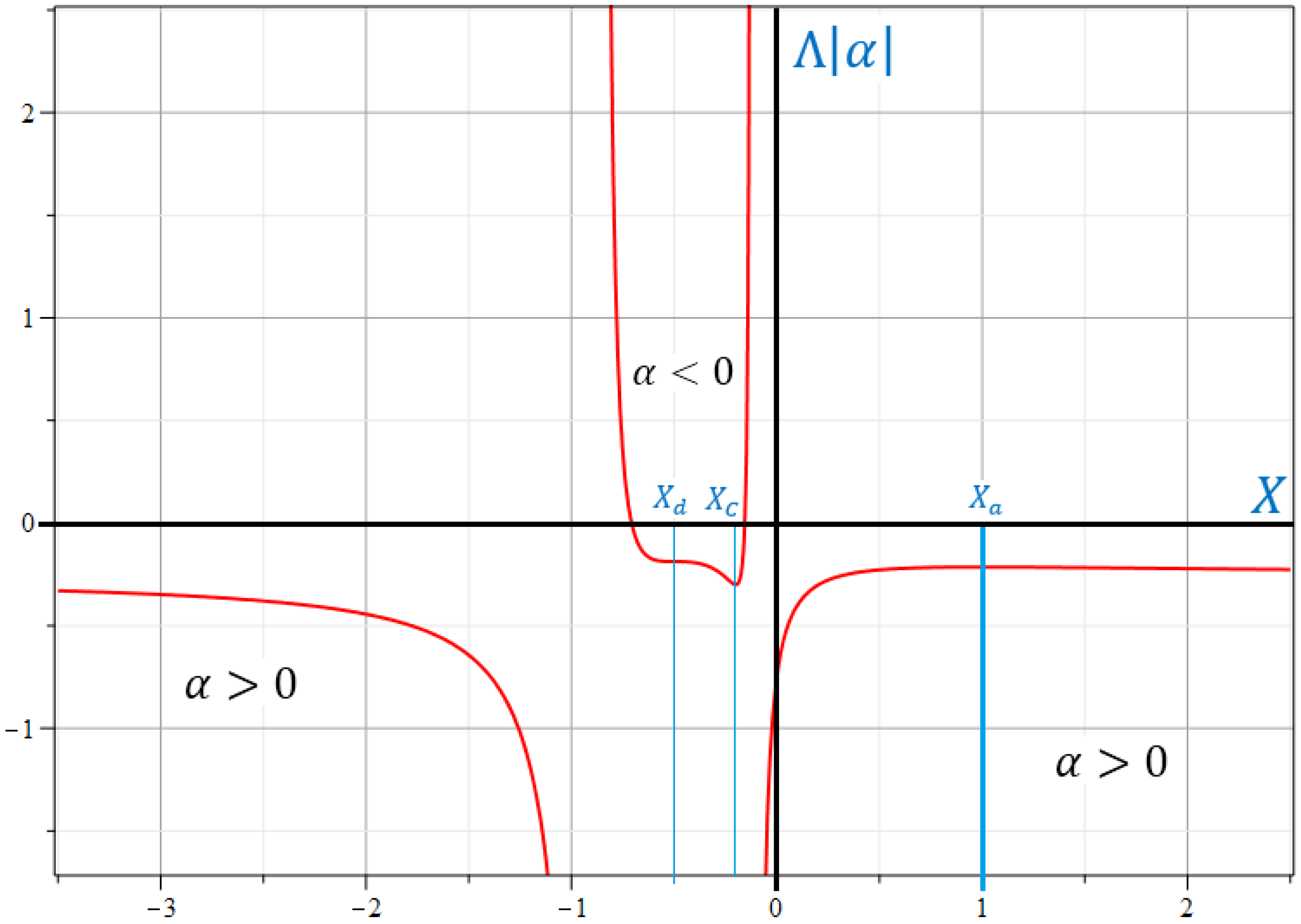
4. Static Analogs of Cosmological Solutions

Now, we deal with the static case by considering the set of Equations (3) and (4) on the manifold (5) with the following ansatz:

$$\begin{array}{c}\hfill g^{\left(10\right)}=du\otimes du+a_3^2\left(u\right)g^{\left(3\right)}+a_6^2\left(u\right)g^{\left(6\right)},\end{array}$$

(71)

$$\begin{array}{c}\hfill A={\omega }^{\left(6\right)},\end{array}$$

(72)

where u is a spatial coordinate and $g^{\left(3\right)}=-dt\otimes dt+d{x}^1\otimes d{x}^1+d{x}^2\otimes d{x}^2,$ is a flat pseudo-Eucleadean metric on ${\mathbb{R}}^3$. $g^{\left(6\right)}$ is the Calabi–Yau metric on K, and ${\omega }^{\left(6\right)}$ is the spin connection 1-form on K defined in a previous section.

The Yang–Mills equations are satisfied identically as in the previous case.

Now, we denote

$$H\left(u\right)\equiv {\dot{a}}_3/a_3,h\left(u\right)\equiv {\dot{a}}_6/a_6,$$

(73)

where, in this section, we denote $\dot{a}\equiv \frac{da}{du}$.

Then, Equation (3) in the ansatz (71) and (72) may be written as follows:

$$\begin{array}{c}\hfill B_0-2\Lambda +\alpha B_1=0,\end{array}$$

(74)

$$\begin{array}{c}\hfill \frac{d{\overline{L}}_H}{du}+(3H+6h){\overline{L}}_H-L_0=0,\end{array}$$

(75)

$$\begin{array}{c}\hfill \frac{d{\overline{L}}_h}{du}+(3H+6h){\overline{L}}_h-L_0=0,\end{array}$$

(76)

where

$$\begin{array}{c}\hfill {\overline{L}}_0=B_0+2\Lambda +\frac{1}{3}\alpha B_1,\end{array}$$

(77)

$$\begin{array}{c}\hfill {\overline{L}}_H=2B_H+\frac{4}{3}\alpha A_H,\end{array}$$

(78)

$$\begin{array}{c}\hfill {\overline{L}}_h=2B_h+\frac{4}{3}\alpha A_h,\end{array}$$

(79)

$B_0,B_H,B_h,B_1$ are defined in (20)–(23), and $A_H,A_h$ are defined in (24), (25), respectively.

As we see, the equations of motion for “Hubble-like” parameters (73) in static case may be obtained from cosmological ones (of Section 3) just by replacement

$$\alpha \mapsto -\alpha ,\Lambda \mapsto -\Lambda .$$

(80)

The dimensionless parameter $\lambda =\Lambda \alpha$ is invariant under this replacement.

Here, we consider the case when “Hubble-like” parameters are constant, i.e.,

$$H\left(u\right)=H=\mathrm{const},h\left(u\right)=h=\mathrm{const},$$

(81)

or, equivalently,

$$a_3\left(u\right)=exp\left(Hu\right),a_6\left(u\right)=exp\left(hu\right).$$

(82)

We obtain a set of polynomial equations

$$\begin{array}{c}\hfill B_0-2\Lambda +\alpha B_1=0,\end{array}$$

(83)

$$\begin{array}{c}\hfill (3H+6h){\overline{L}}_H-{\overline{L}}_0=0,\end{array}$$

(84)

$$\begin{array}{c}\hfill (3H+6h){\overline{L}}_h-{\overline{L}}_0=0,\end{array}$$

(85)

where polynomials ${\overline{L}}_0,{\overline{L}}_H,$ and ${\overline{L}}_h$ are defined by relationships (77)–(79), respectively.

Here, we consider a slightly more general case.

$$H\ne 0.$$

(86)

As in the previous section, we impose the conditions (34) and reduce the relationships (83)–(85) to the set of two equations [26]

$$\begin{array}{c}\hfill \overline{E}=3H^2+6h^2-{(3H+6h)}^2-2\Lambda \\ \hfill +\alpha [144H^{3}h+1080H^2{h}^2+1440H{h}^3+360h^4]=0,\end{array}$$

(87)

$$Q=2H^2+20Hh+20h^2=\frac{1}{2\alpha }.$$

(88)

Using Equation (88) and restriction (86), we obtain

$$H={\epsilon }_0{\left(2\alpha \mathcal{P}\right)}^{-1/2},$$

(89)

where ${\epsilon }_0=\pm 1$, and quadratic polynomial $\mathcal{P}=\mathcal{P}\left(x\right)$ ($x=h/H$) is defined in (38).

Here, we obtain

$$\alpha \mathcal{P}>0,$$

(90)

instead of (40).

According to Equation (90), we obtain in the static case

$$x_{-}<x<x_{+}\mathrm{for}\alpha <0,$$

(91)

and

$$x<x_{-}\mathrm{or}x>x_{+}\mathrm{for}\alpha >0.$$

(92)

(The real numbers $x_{\pm }$ are defined in (44)).

We obtain that the main Equations (43) and (50) for the ratio $x=h/H$ are unchanged in the static case.

Thus, for $\lambda \ne -21/80$ and restrictions (34), (86) imposed, we obtain exact solutions for H and h, which are given by the formulae (52), (89) and (90). For $\lambda =-21/80$, we should use (62) instead of (52).

Graphical analysis. The graphical representation of $\Lambda \left|\alpha \right|$ upon $x=h/H$ in the static case is presented at Figure 3. Here, we use the relationship

$$\Lambda \left|\alpha \right|=\lambda \mathrm{sgn}\left(\alpha \right)=f\left(x\right)\frac{(2+20x+20x^2)}{|2+20x+20x^2|},$$

(93)

in agreement with (90). It follows from Figure 3 that real solutions take place if

$$\Lambda \left|\alpha \right|\ge -{\lambda }_c=-3/10,$$

(94)

for $\alpha <0$ and

$$\Lambda \left|\alpha \right|<{\lambda }_a=-3/14,$$

(95)

for $\alpha >0$.

In the static case, real solutions for $\Lambda =0$ exist only if $\alpha <0$.

Stability. Using the results of Ref. [26], we can analyse the stability of static solutions under consideration obeying $x=h/H\ne x_i$, $i=a,c,d$, where $x_a=1$, $x_c=-\frac{1}{5}$, $x_d=-\frac{1}{2}$.

The solutions are stable for $H>0$ and $u\to +\infty$ if (i) $x>x_d=-1/2$ and unstable if (ii) $x<x_d=-1/2$. For $H>0$ and $u\to -\infty$, they are stable for (i) $x<x_d=-1/2$ and unstable if (ii) $x>x_d=-1/2$.

The solutions are stable for $H<0$ and $u\to +\infty$ if (i) $x<x_d=-1/2$ and unstable if (ii) $x>x_d=-1/2$. For $H<0$ and $u\to -\infty$, they are stable for (i) $x>x_d=-1/2$ and unstable if (ii) $x<x_d=-1/2$.

5. Conclusions

Here, we have considered an Einstein–Gauss–Bonnet–Yang–Mills–$\Lambda$ gravitational model in the dimension $D=10$ with a non-zero constant $\alpha$ coupled to a sum of Yang–Mills and Gauss–Bonnet terms.

We have studied so-called cosmological-type solutions with the metrics (1) defined on product manifolds $M=\mathbb{R}\times {\mathbb{R}}^3\times K$, where $w=\pm 1$, ${\mathbb{R}}^3$ is a flat $3d$ subspace with the metric $g^{\left(3\right)}$, and K is a $6d$ Ricci-flat Calabi–Yau manifold with the metric $g^{\left(6\right)}$. The gauge field 1-form was considered to be coinciding with spin connection 1-form on K: $A={\omega }^{\left(6\right)}$.

For $w=+1$, $\chi =t$, we have obtained exact cosmological solutions with exponential dependence of scale factors (upon the t-variable), governed by two non-coinciding Hubble-like parameters, $H>0$ and h, corresponding to factor spaces of dimensions 3 and 6, respectively, when the following restriction: $3H+6h\ne 0$ is used (excluding the solutions with a constant volume factor).

Static analogs of cosmological solutions ($w=-1$, $\chi =u$) with exponential dependence of scale factors and non-coinciding “Hubble-like” parameters $H\ne 0$ and h, obeying $3H+6h\ne 0$, are also presented here.

We have also outlined the stability of the solutions in the cosmological case (for $t\to +\infty$, Section 3) and in the static case for ($u\to \pm \infty$, Section 4) and have singled out “islands” of stable/non-stable solutions.

Some cosmological applications of the model ($w=1$) may be of interest in the context of the dark energy problem and problems of stability/variation of gravitational constant. For the static case ($w=-1$), possible applications of the obtained solutions may be a subject of a further research, aimed at a search of topological black hole solutions (with a flat horizon) or wormhole solutions which are coinciding asymptotically (for $u\to \pm \infty$) with our solutions.

References

1. Zwiebach, B. Curvature squared terms and string theories. Phys. Lett. B 1985, 156, 315. [Google Scholar] [CrossRef]
2. Fradkin, E.S.; Tseytlin, A.A. Effective action approach to superstring theory. Phys. Lett. B 1985, 160, 69–76. [Google Scholar] [CrossRef] [Green Version]
3. Gross, D.; Witten, E. Superstring modifications of Einstein’s equations. Nucl. Phys. B 1986, 277, 1. [Google Scholar] [CrossRef]
4. Gross, D.; Harvey, J.; Martinec, E.; Rohm, R. Heterotic String. Phys. Rev. Lett. 1984, 54, 502. [Google Scholar] [CrossRef] [PubMed]
5. Ishihara, H. Cosmological solutions of the extended Einstein gravity with the Gauss-Bonnet term. Phys. Lett. B 1986, 179, 217. [Google Scholar] [CrossRef]
6. Deruelle, N. On the approach to the cosmological singularity in quadratic theories of gravity: The Kasner regimes. Nucl. Phys. B 1989, 327, 253–266. [Google Scholar] [CrossRef] [Green Version]
7. Nojiri, S.; Odintsov, S.D. Introduction to Modified Gravity and Gravitational Alternative for Dark Energy. Int. J. Geom. Meth. Mod. Phys. 2007, 4, 115–146. [Google Scholar] [CrossRef] [Green Version]
8. Elizalde, E.; Makarenko, A.; Obukhov, V.; Osetrin, K.; Filippov, A. Stationary vs. singular points in an accelerating FRW cosmology derived from six-dimensional Einstein–Gauss–Bonnet gravity. Phys. Lett. B 2007, 644, 1–6. [Google Scholar] [CrossRef] [Green Version]
9. Bamba, K.; Guo, Z.-K.; Ohta, N. Accelerating Cosmologies in the Einstein-Gauss-Bonnet Theory with a Dilaton. Prog. Theor. Phys. 2007, 118, 879–892. [Google Scholar] [CrossRef] [Green Version]
10. Toporensky, A.; Tretyakov, P. Power-law anisotropic cosmological solution in 5+1 dimensional Gauss–Bonnet gravity. Grav. Cosmol. 2007, 13, 207–210. [Google Scholar]
11. Pavluchenko, S.A.; Toporensky, A.V. A note on differences between (4+1)- and (5+1)-dimensional anisotropic cosmology in the presence of the Gauss-Bonnet term. Mod. Phys. Lett. A 2009, 24, 513–521. [Google Scholar] [CrossRef] [Green Version]
12. Pavluchenko, S.A. General features of Bianchi-I cosmological models in Lovelock gravity. Phys. Rev. D 2009, 80, 107501. [Google Scholar] [CrossRef] [Green Version]
13. Kirnos, I.; Makarenko, A.; Pavluchenko, S.; Toporensky, A. The nature of singularity in multidimensional anisotropic Gauss-Bonnet cosmology with a perfect fluid. Gen. Rel. Grav. 2010, 42, 2633–2641. [Google Scholar] [CrossRef] [Green Version]
14. Ivashchuk, V.D. On anisotropic Gauss-Bonnet cosmologies in (n + 1) dimensions, governed by an n-dimensional Finslerian 4-metric. Grav. Cosmol. 2010, 16, 118–125. [Google Scholar] [CrossRef] [Green Version]
15. Ivashchuk, V.D. On cosmological-type solutions in multi-dimensional model with Gauss-Bonnet term. Int. J. Geom. Meth. Mod. Phys. 2010, 7, 797–819. [Google Scholar] [CrossRef] [Green Version]
16. Maeda, K.-I.; Ohta, N. Cosmic acceleration with a negative cosmological constant in higher dimensions. J. High Energy Phys. 2014, 2014, 95. [Google Scholar] [CrossRef] [Green Version]
17. Chirkov, D.; Pavluchenko, S.; Toporensky, A. Exact exponential solutions in Einstein–Gauss–Bonnet flat anisotropic cosmology. Mod. Phys. Lett. A 2014, 29, 1450093. [Google Scholar] [CrossRef] [Green Version]
18. Chirkov, D.; Pavluchenko, S.; Toporensky, A. Non-constant volume exponential solutions in higher-dimensional Lovelock cosmologies. Gen. Rel. Grav. 2015, 47, 137. [Google Scholar] [CrossRef] [Green Version]
19. Pavluchenko, S.A. Stability analysis of exponential solutions in Lovelock cosmologies. Phys. Rev. D 2015, 92, 104017. [Google Scholar] [CrossRef] [Green Version]
20. Pavluchenko, S.A. Cosmological dynamics of spatially flat Einstein-Gauss-Bonnet models in various dimensions: Low-dimensional Λ-term case. Phys. Rev. D 2016, 94, 084019. [Google Scholar] [CrossRef] [Green Version]
21. Canfora, F.; Giacomini, A.; Pavluchenko, S.; Toporensky, A. Friedmann Dynamics Recovered from Compactified Einstein–Gauss–Bonnet Cosmology. Grav. Cosmol. 2018, 24, 28–38. [Google Scholar] [CrossRef] [Green Version]
22. Ivashchuk, V.D. On stability of exponential cosmological solutions with non-static volume factor in the Einstein–Gauss–Bonnet model. Eur. Phys. J. C 2016, 76, 431. [Google Scholar] [CrossRef] [Green Version]
23. Fomin, I.; Chervon, S. A new approach to exact solutions construction in scalar cosmology with a Gauss–Bonnet term. Mod. Phys. Lett. A 2017, 32, 1750129. [Google Scholar] [CrossRef] [Green Version]
24. Ivashchuk, V.D.; Kobtsev, A.A. Stable exponential cosmological solutions with 3- and l-dimensional factor spaces in the Einstein–Gauss–Bonnet model with a Λ-term. Eur. Phys. J. C 2018, 78, 100. [Google Scholar] [CrossRef] [Green Version]
25. Ivashchuk, V.D.; Kobtsev, A.A. Exponential cosmological solutions with two factor spaces in EGB model with Λ = 0 revisited. Eur. Phys. J. C 2019, 79, 824. [Google Scholar] [CrossRef] [Green Version]
26. Ivashchuk, V.D. On Stability of Exponential Cosmological Type Solutions with Two Factor Spaces in the Einstein–Gauss–Bonnet Model with a Λ-Term. Grav. Cosmol. 2020, 20, 16–21. [Google Scholar] [CrossRef]
27. Riess, A.G.; Filippenko, A.V.; Challis, P.; Clocchiatti, A.; Diercks, A.; Garnavich, P.M.; Gilliland, R.L.; Hogan, C.J.; Jha, S.; Kirshner, R.P.; et al. Observational evidence from supernovae for an accelerating universe and a cosmological constant. Astron. J. 1998, 116, 1009–1038. [Google Scholar] [CrossRef] [Green Version]
28. Perlmutter, S.; Aldering, G.; Goldhaber, G.; Knop, R.A.; Nugent, P.; Castro, P.G.; Deustua, S.; Fabbro, S.; Goobar, A.; Groom, D.E. Measurements of Ω and Λ from 42 high redshift supernovae. Astrophys. J. 1999, 517, 565–586. [Google Scholar] [CrossRef]
29. Nojiri, S.; Odintsov, S.D.; Oikonomou, V.K. Modified Gravity Theories on a Nutshell: Inflation, Bounce and Late-time Evolution. Phys. Rept. 2017, 692, 1–104. [Google Scholar] [CrossRef] [Green Version]
30. Abbas, G.; Momeni, D.; Ali, M.A.; Myrzakulov, R.; Qaisar, S. Anisotropic compact stars in f(G) gravity. Astrophys. Space Sci. 2015, 357, 158. [Google Scholar]
31. Benetti, M.; da Costa, S.S.; Capozziello, S.; Alcaniz, J.; De Laurentis, M. Various characteristics of transition energy for nearly symmetric colliding nuclei. Int. J. Mod. Phys. 2018, 27, 1850084. [Google Scholar] [CrossRef] [Green Version]
32. Nojiri, S.; Odintsov, S.D.; Oikonomou, V.K. Unifying Inflation with Early and Late-time Dark Energy in F(R) Gravity. Phys. Dark Universe 2020, 29, 100602. [Google Scholar] [CrossRef]
33. Vasilev, T.B.; Bouhmadi-Lopez, M.; Martin-Moruno, P. Classical and Quantum f(R) Cosmology: The Big Rip, the Little Rip and the Little Sibling of the Big Rip. Universe 2021, 7, 288. [Google Scholar] [CrossRef]
34. Vasilev, T.B.; Bouhmadi-Lopez, M.; Martin-Moruno, P. f(G,TαβTαβ) theory and complex cosmological structures. Phys. Dark Universe 2022, 36, 101015. [Google Scholar]
35. Fazlollahi, H.R. Energy–momentum squared gravity and late-time Universe. Eur. Phys. J. Plus 2023, 138, 211. [Google Scholar] [CrossRef]
36. Boulware, D.G.; Deser, S. String Generated Gravity Models. Phys. Rev. Lett. 1985, 55, 2656. [Google Scholar] [CrossRef] [PubMed] [Green Version]
37. Wheeler, J.T. Symmetric Solutions to the Gauss-Bonnet Extended Einstein Equations. Nucl. Phys. B 1986, 268, 737. [Google Scholar] [CrossRef]
38. Wheeler, J.T. Symmetric Solutions to the Maximally Gauss-Bonnet Extended Einstein Equations. Nucl. Phys. B 1986, 273, 732. [Google Scholar] [CrossRef] [Green Version]
39. Wiltshire, D.L. Spherically Symmetric Solutions of Einstein-maxwell Theory With a Gauss-Bonnet Term. Phys. Lett. B 1986, 169, 36–40. [Google Scholar] [CrossRef]
40. Cai, R.-G. Gauss-Bonnet black holes in AdS spaces. Phys. Rev. D 2002, 65, 084014. [Google Scholar] [CrossRef] [Green Version]
41. Cvetic, M.; Nojiri, S.; Odintsov, S. Black hole thermodynamics and negative entropy in de Sitter and anti-de Sitter Einstein-Gauss-Bonnet gravity. Nucl. Phys. B 2002, 628, 295. [Google Scholar] [CrossRef] [Green Version]
42. Garraffo, C.; Giribet, G. The Lovelock Black Holes. Mod. Phys. Lett. A 2008, 23, 1801. [Google Scholar] [CrossRef]
43. Charmousis, C. Higher order gravity theories and their black hole solutions. Lect. Notes Phys. 2009, 769, 299. [Google Scholar]
44. Antoniou, G.; Bakopoulos, A.; Kanti, P. Black-Hole Solutions with Scalar Hair in Einstein-Scalar-Gauss-Bonnet Theories. Phys. Rev. D 2018, 97, 084037. [Google Scholar] [CrossRef] [Green Version]
45. Bronnikov, K.A.; Kononogov, S.A.; Melnikov, V.N. Brane world corrections to Newton’s law. Gen. Rel. Grav. 2006, 38, 1215–1232. [Google Scholar] [CrossRef] [Green Version]
46. Tavakoli, Y.; Ardabili, A.K.; Bouhmadi-Lopez, M.; Moniz, P.V. Role of Gauss-Bonnet corrections in a DGP brane gravitational collapse. Phys. Rev. D 2022, 105, 084050. [Google Scholar] [CrossRef]
47. Kanti, P.; Kleihaus, B.; Kunz, J. Wormholes in Dilatonic Einstein-Gauss-Bonnet Theory. Phys. Rev. Lett. 2011, 107, 271101. [Google Scholar] [CrossRef] [Green Version]
48. Barton, S.; Kiefer, C.; Kleihaus, B.; Kunz, J. Symmetric wormholes in Einstein-vector–Gauss–Bonnet theory. Eur. Phys. J. C 2022, 82, 802. [Google Scholar] [CrossRef]
49. Wu, Y.-S.; Wang, Z. Time variation of Newton’s gravitational constant in superstring theories. Phys. Rev. Lett. B 1986, 57, 1978. [Google Scholar] [CrossRef]
50. Ivashchuk, V.D.; Melnikov, V.N. On time variations of gravitational and Yang-Mills constants in a cosmological model of superstring origin. Grav. Cosmol. 2014, 20, 26–29. [Google Scholar] [CrossRef] [Green Version]
51. Candelas, P.; Horowitz, G.T.; Strominger, A.; Witten, E. Vacuum configurations for superstrings. Nucl. Phys. B 1985, 256, 46. [Google Scholar] [CrossRef]
52. Duff, M. Architecture of Fundamental Interactions at Short Distances; Ramond, P., Stora, R., Eds.; Les Houches Lectures: Les Houches, France, 1985; p. 819. [Google Scholar]
53. Cadavid, A.; Ceresole, A.; D’Auria, R.; Ferrara, S. Eleven-dimensional supergravity compactified on Calabi-Yau threefolds. Phys. Lett. B 1995, 357, 76–80. [Google Scholar] [CrossRef] [Green Version]
54. Duff, M.J.; Lu, H.; Pope, C.N.; Sezgin, E. Supermembranes with fewer supersymmetries. Phys. Lett. B 1996, 371, 206–214. [Google Scholar] [CrossRef] [Green Version]
55. Golubtsova, A.A.; Ivashchuk, V.D. Triple M-brane configurations and preserved supersymmetries. Nucl. Phys. B 2013, 872, 289–312. [Google Scholar] [CrossRef] [Green Version]
56. Ivashchuk, V.D. On Supersymmetric M-brane configurations with an R * 1 , 1 /Z2 submanifold. Grav. Cosmol. 2016, 22, 32–35. [Google Scholar] [CrossRef] [Green Version]
57. Witten, L.; Witten, E. Large Radius Expansion of Superstring Compactifications. Nucl. Phys. B 1987, 281, 109. [Google Scholar] [CrossRef]
Figure 1. The graphical representation of moduli function λ = f ( x ) given by relationship (43).
Symmetry 15 00783 g001
Figure 2. The dependence of Λ | α | upon x = h / H in cosmological case. The central branch corresponds to α > 0 . The left and right branches correspond to α < 0 .
Symmetry 15 00783 g002
Figure 3. The dependence of Λ | α | upon x = h / H in static case. The central branch corresponds to α < 0 . The left and right branches correspond to α > 0 .
Symmetry 15 00783 g003
Disclaimer/Publisher’s Note: The statements, opinions and data contained in all publications are solely those of the individual author(s) and contributor(s) and not of MDPI and/or the editor(s). MDPI and/or the editor(s) disclaim responsibility for any injury to people or property resulting from any ideas, methods, instructions or products referred to in the content.