A Brief Introductory Note on the Possible Chaotic Dynamics of the Muon Time Series of Cosmic Rays Measured at Sea Level by a Simple GMT Detector

Abstract

After an investigation of the well-known basic properties of muons conducted by the standard model (SM), this paper presents the results obtained for the phase space reconstruction, for the correlation dimension and for the largest Lyapunov exponent of a muon time series detected for a period of about three years (2019–2021) in an Italian laboratory at the sea level. These results confirm that the dynamics of such a time series is chaotic in nature, and therefore open new perspectives in the study of cosmic rays. In the following studies, we will explore if such muon time series have a mono- or a multifractal regime with a complete analysis of all the parameters that usually involve such studies.

1. Introduction

Primary cosmic rays (CR) are subatomic particles coming from deep space; due to their incoming rate and isotropic distribution, CR time series reordered by detectors have always been regarded as random noise and, thus, a perfect source of true random number generators (TRNGs). The term noise is used to denote any signal that appears random and not predictable. In cryptography or other applications that require pure random variables, cosmic rays give the impression of being a perfect choice. Muons are elementary particles created in the atmosphere by primary CRs. They inherit the distribution and some other features of the primary particles. Many authors have found methods to convert the time interval between two muons crossing a detector to random binary information (e.g., Gamil et al. [1]). Even our own AstroRad software (see later) can calculate Pi from an algorithm based on the “random” time arrival of every muon using the Monte Carlo method. However, in chaos theory, some studies show a new perspective on CR nature, proving that a muon time series may have a chaotic dynamics. This means that cosmic radiation itself has a deterministic origin and could be predictable to a large extent. Presently, we can still choose cosmic rays as TRNGs, but this is a task that can be solved better by quantum computers [2]. Indeed, we have to take into consideration that CRs, in some circumstances, show no stochastic nature at all. Therefore, the aim of our work is to answer to the following question: is the flux of muons, measured at sea level, deterministically chaotic, implying a cosmic ray strange attractor, or is it stochastic, implying they are colored random noise?

2. A Preliminary Survey on Cosmic Rays

Muons are leptons, a group of particles that include electrons, tau particles and their three neutrinos. Muons are created by cosmic rays that are mainly high-energy protons that collide with the nuclei of the atmosphere, where they produce showers of unstable non-elementary pions. They decay into muons. It is accepted that the muon is a particle similar to the electron, but is 200 times heavier and unstable. It decays in microseconds (2.2 × 10⁻⁶ s) into three new particles: an electron, an electron antineutrino and a muon neutrino, according to the following scheme of reaction (Figure 1):

$$\begin{gathered} {\mathsf{\mu }}^{-}\to {\mathrm{e}}^{-}+{\overline{\upsilon }}_{\mathrm{e}}+{\upsilon }_{\mathsf{\mu }} \\ {\mathsf{\mu }}^{+}\to {\mathrm{e}}^{+}+{\upsilon }_{\mathrm{e}}+{\overline{\upsilon }}_{\mathsf{\mu }} \end{gathered}$$

(1)

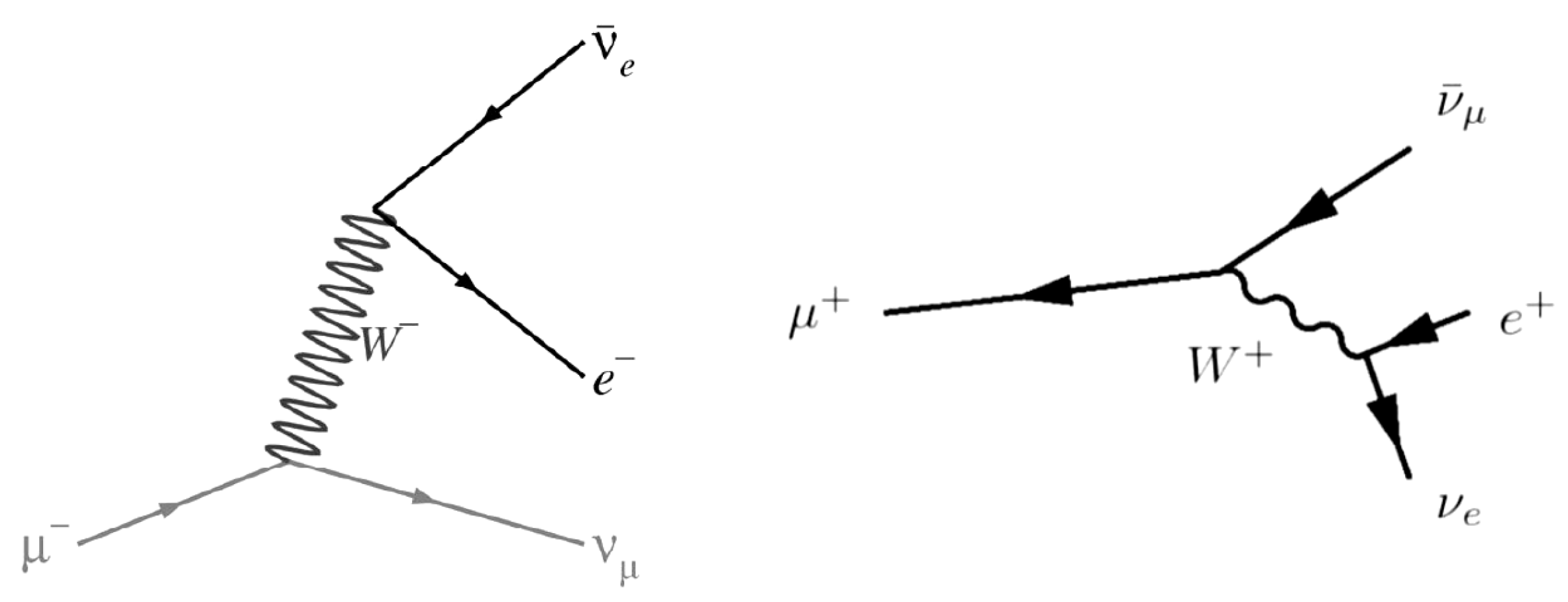
2.1. Muon within the Standard Model of Fundamental Particles

We can analyze the muon decay using the existing theory of the standard model (SM) of fundamental particles. The current SM analyzes all visible matter in galaxies and covers about 4% of the mass of the universe. According to the SM, the remaining 96% of the universe comprises dark matter and dark energy [3].

2.2. Standard Model and Measurement of the Muon Lifetime Value

We may calculate the dimensionless strength of the weak force that we indicate by g_w using some experimental data and the standard model. In the SM, the well-known electromagnetic interaction is related to the weak interaction that is responsible for particle decays, such as muon decay. In the SM, the strength of the instability interaction is denoted by g_w and determines how long a muon exists before it breaks up. The theoretical lifetime formula permits the discovery of the weak coupling constant g_w.

As represented in the so-called Feynman diagrams below, muons (electrically positive or negative) decay through the intermediate emission of W bosons.

The muon lifetime formula for τ as calculated from these diagrams depends on g_w and on masses of W-boson M_W and muon m_μ.

$$\tau =\frac{1}{\mathsf{\Gamma }}={\left(\frac{M_W}{m_{\mu }{g}_w}\right)}^4\frac{\hslash {\left(8\pi \right)}^3}{m_{\mu }{c}^2}$$

(2)

Solving this formula for g_w, we have:

$$g_w=8\sqrt[4]{\frac{3{\pi }^3\widehat{h}}{2\tau m_{\mu }{c}^2}}\frac{M_W}{m_{\mu }}\mathrm{a}=1,$$

(3)

and using our measured lifetime τ together with the rest mass energy of W-boson m_Wc² = 80.4 GeV and of muon m_μc² = 105.7 MeV given by experimental data, it has been estimated that one of the fundamental constants of nature, the dimensionless strength of the weak force g_w = 0.680, with a 4% error when compared with the accepted value of 0.653.

In the SM, electroweak interaction is mediated by photon exchange, while weak force is mediated by heavy bosons. We have:

$$e=g_{w}sin\theta \sqrt{\hslash c{\mathsf{\epsilon }}_0},$$

(4)

as in the standard model [4].

In recent years, the possibility of new physical phenomena beyond the standard model has been disputed. In the SM, it is predicted that muon and tau particles are heavy copies of the electron, and they behave similar to the electron. This identical behavior of the particles, which all belong to the lepton group, is called lepton universality. With the Large Hadron Collider (LHC) detector, researchers are investigating whether the behavior is really the same or whether there are slight deviations. The focus is B-mesons, which are produced in large quantities when energy-rich protons collide at the LHC. These particles only exist for a few fractions of a second. After their decay, in extremely rare cases, this also gives rise to other B-mesons, which then decay into either electrons or muons. The measurement that has just been studied is about the particle decay of B+ mesons.

It has been found that B+ mesons decay somewhat more often into electrons than into muons, although, theoretically, with such decay, the two final states should come about equally often. The result indicates a violation of lepton universality. However not enough data have been accumulated to be able to confirm a new finding. It has been assumed that the symmetry between electrons and muons is shaky. If it were possible to confirm the measurement with further data, this would be a strong indication of new physical phenomena beyond the SM. At the moment, the data calls for explanations and models that go beyond the standard model [5].

3. Experimental Setup

For the measurement of muons, we must remember that such particles, moving at speeds close to the speed of light, enter, slow down, stop, and subsequently decay in matter. Sometimes this happens even in plastic scintillator detectors. When this occurs, each muon determines two light pulses separated by a few microseconds: one pulse originates when it enters the scintillator, and the second one when the muon decays. The pulses can be viewed with an oscilloscope and thus stored on a computer. One can measure the time difference between these correlated pulses, as well as the amplitude of each pulse and the number of pulses over a given time. The voltage pulses are proportional to the particle energy loss in the detector [4].

Details of Our Digital System and Data Acquisition

For our purposes, we only count the number of muons per unit of time and area. To detect only hard cosmic radiation—the muons—our instrument uses at least two stacked sensors in a noted configuration, the so-called coincident circuit invented by Bothe and Rossi in the early 1930s [6]. Muons have great penetrating power in matter, so they can easily cross two or more stacked sensors, while other ionizing particles cannot. In this way, the coincidence method permits the identification of muons among natural ionizing radiation. We used a detector named Astroparticle Muon Detector 5 (AMD5). This instrument is built with two Geiger–Müller tubes (GMT); model SBM20, made in Russia. The two stacked GMTs give the instrument a telescope field of view of about 0.5 sr (in Figure 2, we give the plot of muon an average count, against the sr values); the overall detection surface area is in the order of 8 cm² and with this setup, the relative average rate is usually around 2 counts per minute (cpm). Signals from the GMT sensors are processed by a simple electronic board. The electronics extend the pulse length from each sensor by a certain amount of time (in the order of milliseconds), which is the time window for the coincidence signal. Then, the two signals are sent into a digital “and” gate that provides the coincident pulse. The time window is adjustable to tune different GMTs with different technical parameters and to facilitate different experiments. In the end, the signal is a squared pulse sent to a USB card connected to a personal computer. Every pulse is interpreted and counted as a cosmic ray (muon); our own software called AstroRad gathers the pulses and records several sets of data files at different time resolutions, and a set of data with a time stamp for each particle. The main time-resolution data are cpm, count/5 s, the average count for one whole day, and a dosimetry dataset. Despite the small detection area, over the years the AMD5 detector has proved to be very reliable, and now many instruments of this sort are in use in an Italian CR network called the Astroparticle Detector Array (educational project) [7]. The detectors are set in a vertical position, measuring with a zenithal angle equal to zero. The measurements in time of the muons give the origin to a time series of muons that, stored in a computer, may be studied by the methodology of chaos analysis.

4. Method of Analysis

An investigation of chaotic time series data is done in the following manner. First, a reconstruction of the time series data is required in phase space. To reach this target, the time delay must be reconstructed. This is obtained by calculating the autocorrelation function (ACF) and the average mutual information (AMI). Autocorrelation is calculated by doing the correlation of a signal with a delayed copy of itself as a function of delay. Then, it is evaluated for the first minimum of such a function. Consequently, the AMI function is evaluated by selecting the first time that such function goes to zero. This function estimates the nonlinearity of the given time series. If both the values of the time delay coincide, one selects the value indicated; otherwise, the value of the time delay will be that of the AMI. Thus, the value of false nearest neighbors (FNN) is determined. This is the value under which the FNN goes under a selected threshold. In our case, we selected 5% as the threshold. In this way, we know the values of time delay and of the dimensional space in which our time series goes and, consequently, the phase space has been reconstructed. In the subsequent developments, the fractal dimension in such given space is calculated using the correlation dimension (CD), whose value is given in the text. The value of the correlation dimension is given as the average of the values calculated among the limits of 5 and 10 of the estimated values of the embedding dimension. Finally, the largest Lyapunov exponent is estimated by the proper algorithm of the Leonov method and is positive only if the given series is actually chaotic. The use of surrogate data estimates the presence of determinism in our time series data. If the results are the same as the raw data, we have reasons to suspect our conclusion. The time series data are simply shuffled, just as we shuffle a deck of cards. This operation preserves the probability distribution but produces a very different correlation function and other data.

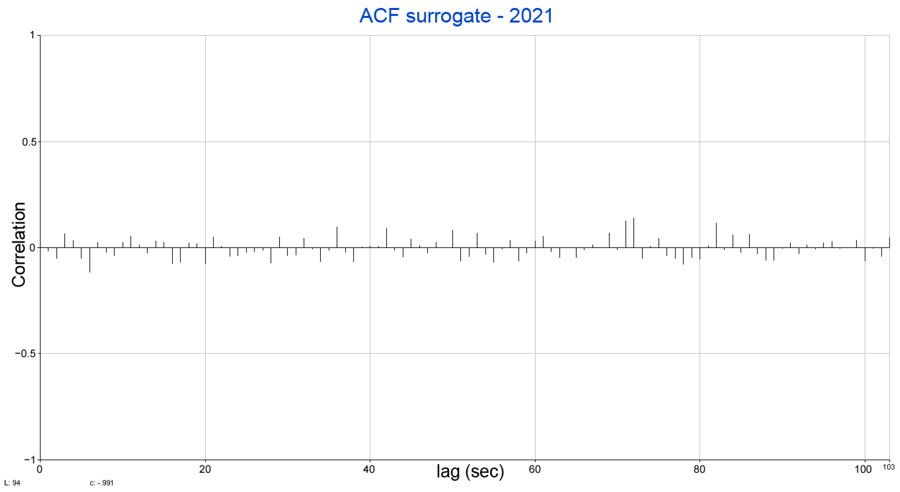
4.1. CHAOS Analysis of Muon Time Series

The data cover several years, from 2019 to 2021, and it is well known that the muon rate depends on atmospheric properties, pressure, temperature at the 100 mb level, and properties of the heliosphere, its various sectors, the strength of the solar wind and Forbush decreases. We know very little about such questions to arrive at a model for muon rate, and this will be the object of future detailed research. In Figure 3, we report the raw data and relative surrogate data in the years 2019, 2020 and 2021.

In Figure 4, we give the probability distribution of the raw data of muon time series in the years 2019, 2020 and 2021.

The aim of the present initial study is to ascertain that nonlinear features are present in our raw data. Subsequent studies will attempt to give a more articulated answer to the above-posed questions. To perform a preliminary analysis, a nonlinear approach is required. The nonlinear analysis of measured data is generally based on so-called embedding, which is the reconstruction of the signal in multidimensional phase space. For this purpose, we have to calculate the time delay that is performed estimating the autocorrelation function (ACF) and the average mutual information (AMI) of the given time series and for surrogate data. We have calculated the ACF and the AMI for each single muon time series that was measured at the level of sea in the years 2019, 2020 and 2021. Such analysis was used to check for the presence of nonlinear contributions in the examined time series data and to evaluate the proper time delay. The results are given in Figure 5, Figure 6, Figure 7, Figure 8, Figure 9 and Figure 10. In Figure 11, we give the results of the AMI for the 2019, 2020 and 2021 muon time series and surrogate data in the same years 2019–2021. All the results confirm that we are in the presence of a muon series with nonlinear contributions. The time delay and the behaviors of the two graphs were different, with values near zero for the given muon time series in 2019, 2020 and 2021 of the shuffled data, with slight differences for the ACF. Therefore, we concluded that nonlinear contributions are present in our series, and the selected time delay is tau = 3 [8,9,10,11,12].

The AMI between two random variables measures the nonlinear relationship between them. It indicates how much information can be obtained from a random variable by observing another random variable. The following formula shows the calculation of the AMI between two random variables X and Y with nonlinear dependence:

$$I\left(X;Y\right)={\displaystyle \sum }_{y\in Y}{\displaystyle \sum }_{x\in X}{p}_{\left(X,Y\right)}log\left(\frac{{p_{\left(X,Y\right)}}^{\left(x,y\right)}}{{p_X}^{\left(x\right)}{p_Y}^{\left(y\right)}}\right),$$

(5)

where p_X^(x)and p_Y^(y) are the marginal probability density functions and p_(X,Y)^(x,y) the joint probability density function. In Figure 11, we report the results of the AMI obtained by the muon time series for raw data and surrogate data. The obtained time delay is 4 as the first minimum of the function [8,9,10,11,12]. For the ACI, the time delay is the first zero of the ACI function, and for the AMI, the time delay is the first minimum of this function. Our criterion to verify nonlinear presence is as follows: for the surrogate data, it is stated as nonlinearity if the mutual difference between the original data and surrogate data is greater than 10%. We have obtained differences varying between the 11 and 15%. Therefore, the nonlinearity of the data seems to be confirmed.

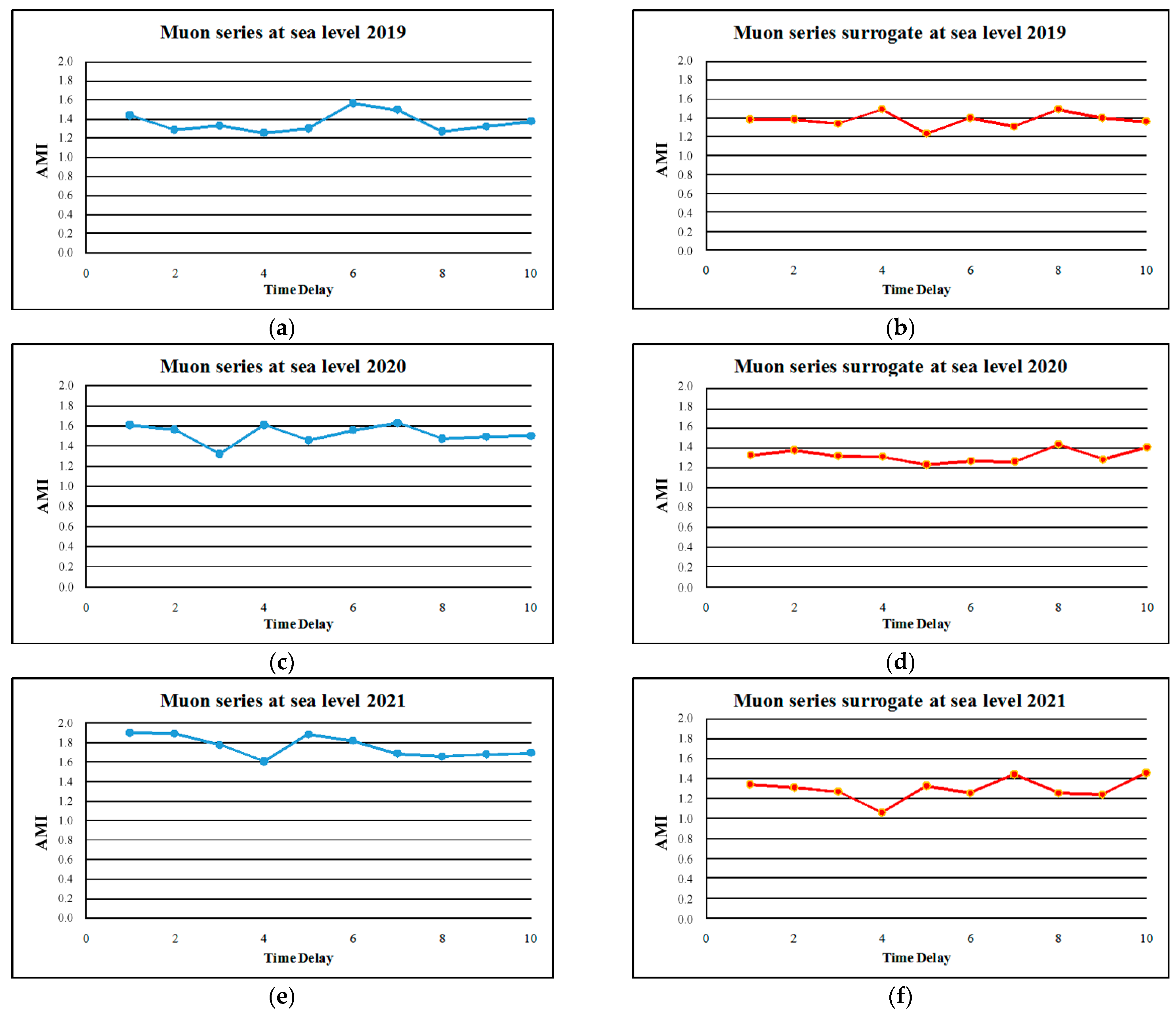
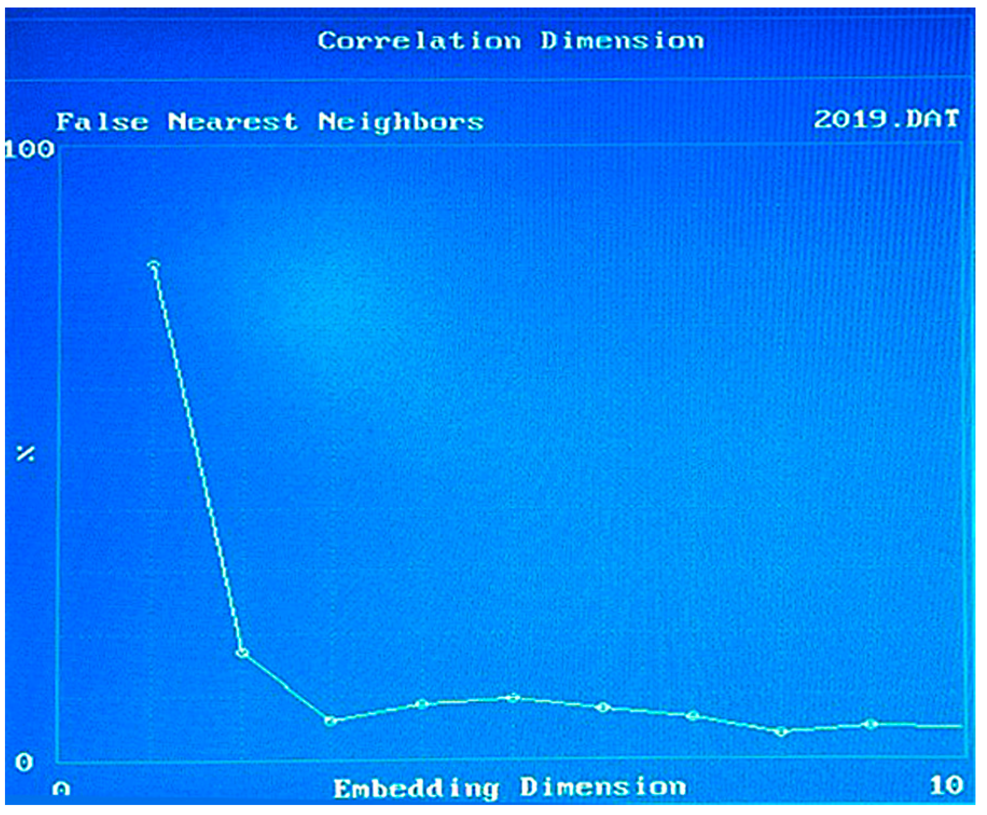
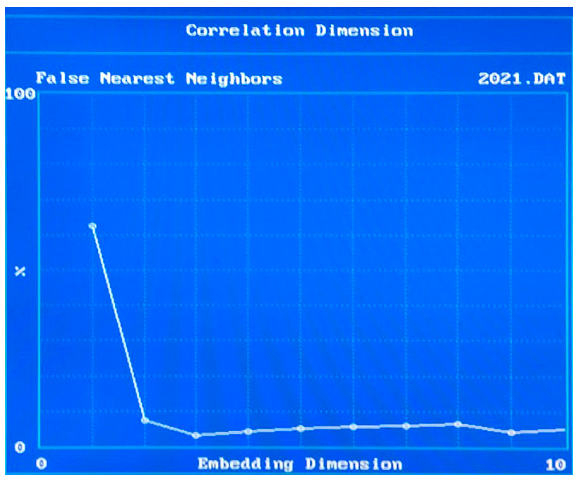
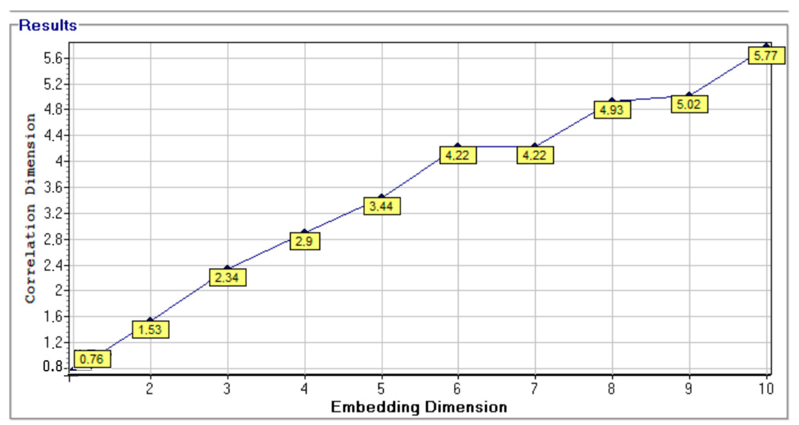
4.2. Phase Space Reconstruction

Within abstract algebra, the false nearest neighbor algorithm estimates the embedding dimension. This idea originates from Kennel et al., 1992, who elaborated on this approach. The basic idea is to examine how the number of neighbors of a point along a signal trajectory change with increasing embedding dimension. In a too-low embedding dimension, many of the neighbors will be false, but in an appropriate embedding dimension or higher, the neighbors are real. After increasing dimensions, the false neighbors will no longer be neighbors. The algorithm is able to examine how the number of neighbors change as a function of dimension, and thus an appropriate embedding can be determined [13]. We have used the criterion of false nearest neighbors to reconstruct the phase space of the given muon time series. Given a time series {xi}, where i = 1, 2, …, N, the phase space behavior is reconstructed using the method of standard delay-coordinate embedding, where the vectors of phase space reconstruction are expressed as below:

$$X\left(t_i\right)=\left[x\left(t_i\right),x\left(t_i+\tau \right),\dots ,x\left(t_i+\left(m-1\right)\tau \right)\right],$$

(6)

where τ is the time delay, and m is the embedded dimension. The dynamic properties of the systems are studied by the reconstruction of the phase space, if m = 2D₂ + 1, and where D₂ is the fractal dimension of the system [10,11,12]. To reconstruct the attractor, the estimation of the embedding dimension m and the embedding delay τ are essential. The method of autocorrelation function is used for the determination of the delay, τ, as the delay causing the value of (1 − 1/e) is its initial of the autocorrelation function [10,11,12,13]. Soon afterwards, the AMI criterion must be used for the determination of time delay in the presence of nonlinear dynamics. The embedding dimension m was estimated using the Grassberger–Procaccia algorithm method proposed by Grassberger [11,14], which is suitable for shorter time series.

We have obtained the following results (Figure 12, Figure 13 and Figure 14) for the original data with a cut-off of 5%. The reconstructed dimension was D = 3. This result may suggest that we are in the presence of a chaotic dynamic system with only three variables to account for. In any of the given time series, we have effectuated the comparison between raw data and shuffled data. Attractors are subsets of the phase space of a dynamical system. In the 1960s, attractors were often considered to be simple geometric subsets of the phase space, as points, lines, surfaces, and simple regions of three-dimensional space. More complex attractors that cannot be categorized as simple geometric subsets were known at the time, but were considered to be anomalies [14]. Smale emphasized for the first time that they are robust objects, and that the attractor has the structure of a Cantor set. Two simple attractors are a fixed point and a limit cycle. Attractors can take on many other geometric shapes that are phase space subsets. However, when these sets cannot be easily described as simple combinations of fundamental geometric objects, then the attractor is called a strange attractor. It is an attractor for which the approach to its final point in phase space is chaotic. Our analysis seems to demonstrate that we are in the presence of a strange attractor that has fundamental chaotic properties.

We come now to analyze the correlation dimension (CD), which is the measure of the attractor dimension. The CD is a measure of the dimensionality of the space occupied by a set of random points, often referred to as a type of fractal dimension. It is indicated by D₂ and it is calculated by the following formula:

$$D_2=\underset{R\to 0}{\lim }\frac{lnC\left(R,d\right)}{lnR},$$

(7)

where:

$$\begin{gathered} C\left(R,d\right)={\sum }_{i,j=1;i<j}^N\theta \left(R-\left|y_i-y_j\right|\right), \\ \theta \left(x\right)=1 \mathrm{for} x > 0, \theta \left(x\right)=0 \mathrm{otherwise}. \end{gathered}$$

(8)

For our muon time series from the years 2019, 2020 and 2021, we obtained the following results, given in Figure 15, Figure 16 and Figure 17, with other results given for the surrogate data in Figure 18, Figure 19 and Figure 20.

The calculated correlation dimension has better saturation, respectively:

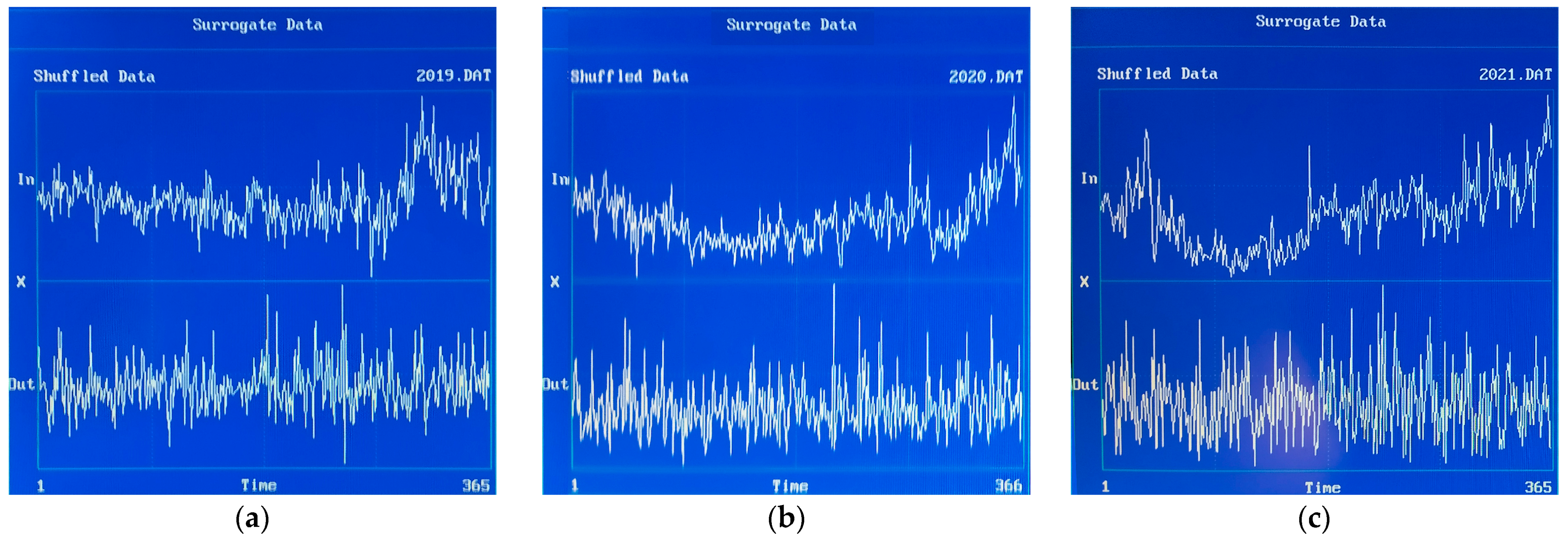
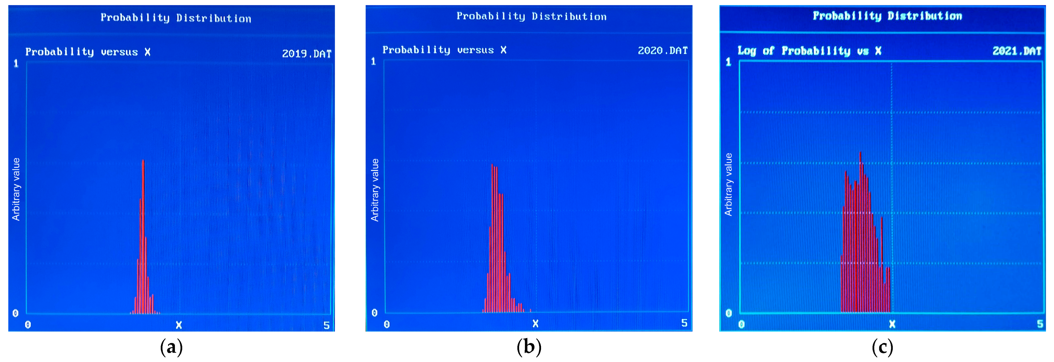
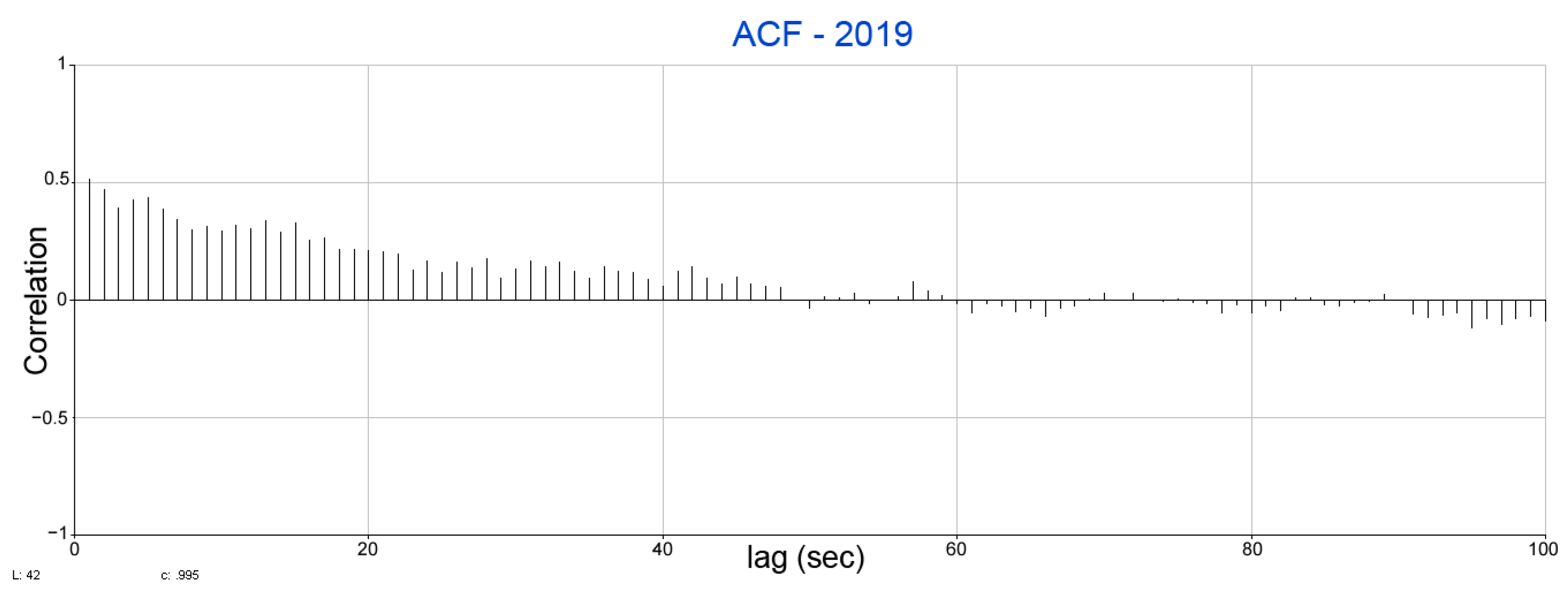
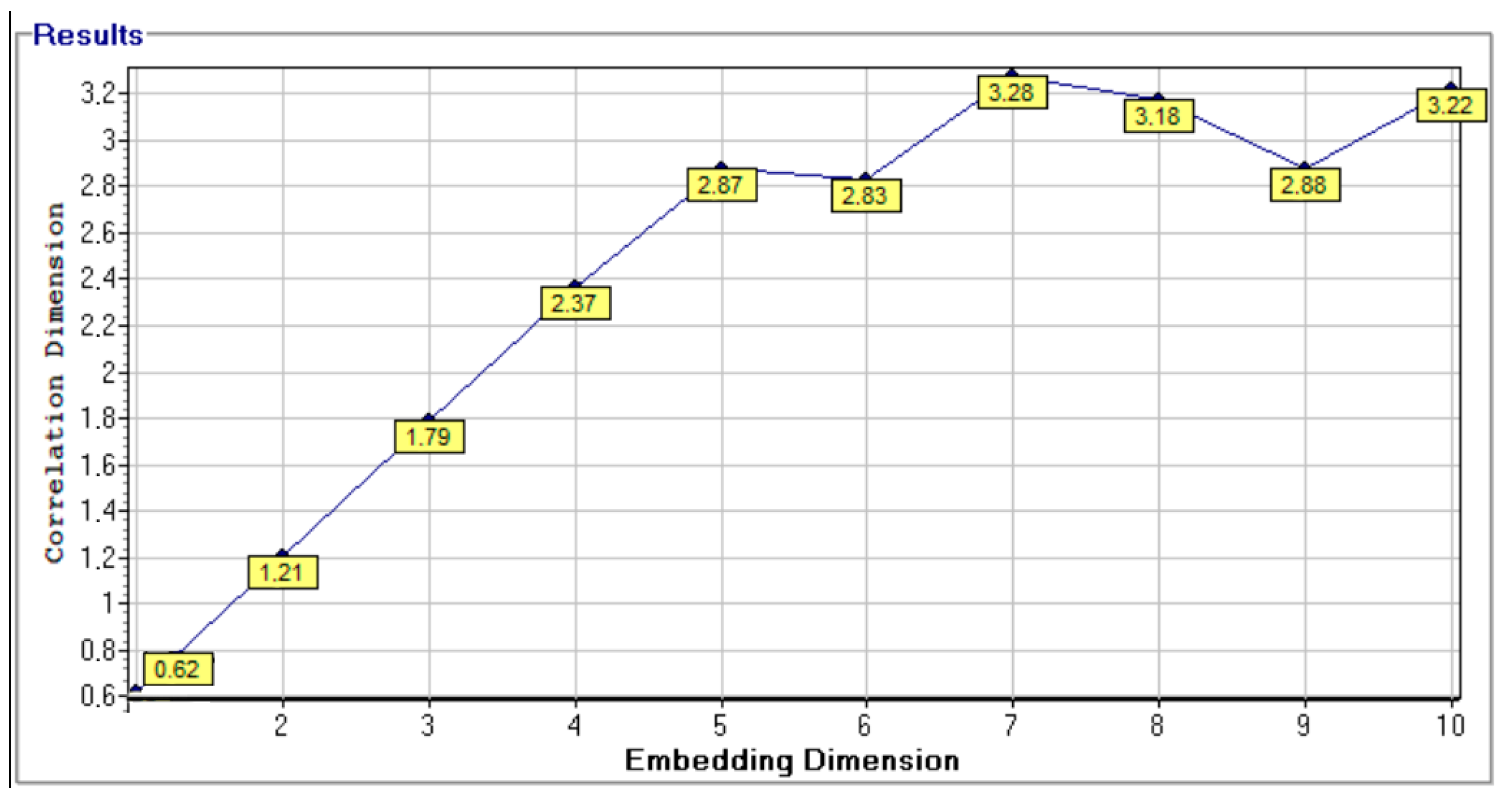
• Data of muon time series in 2019: CD = 2.425 ± 0.921
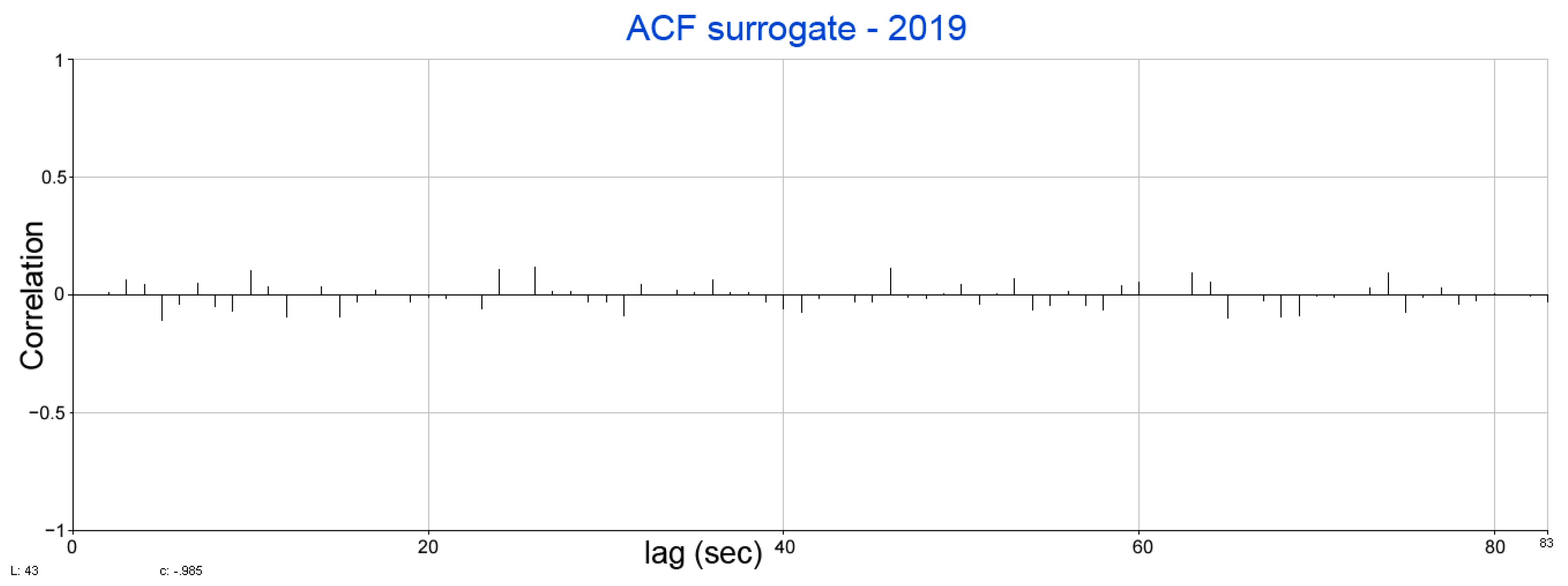
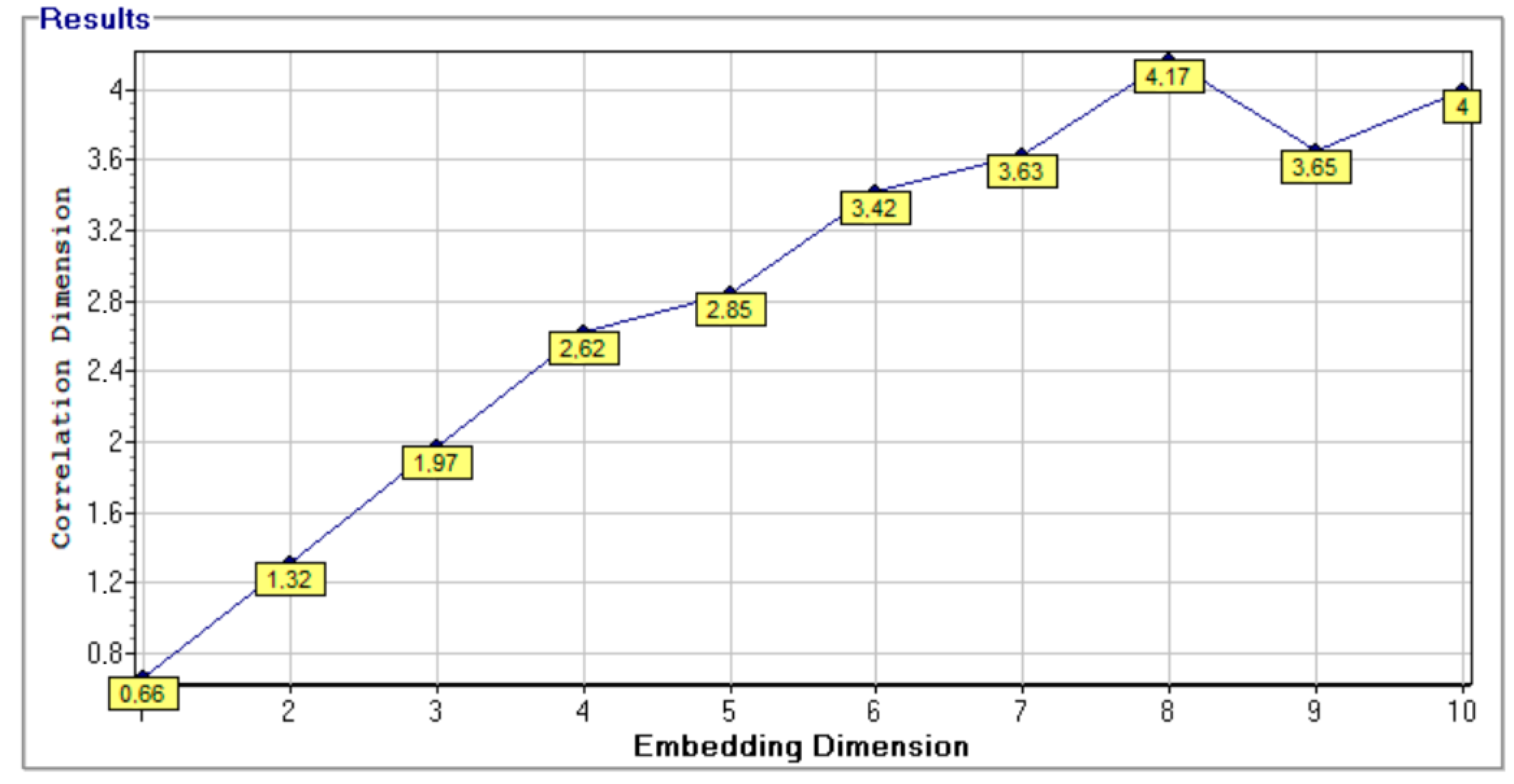
• Data of surrogate of muon time series in 2019: CD = 2.736 ± 1.132
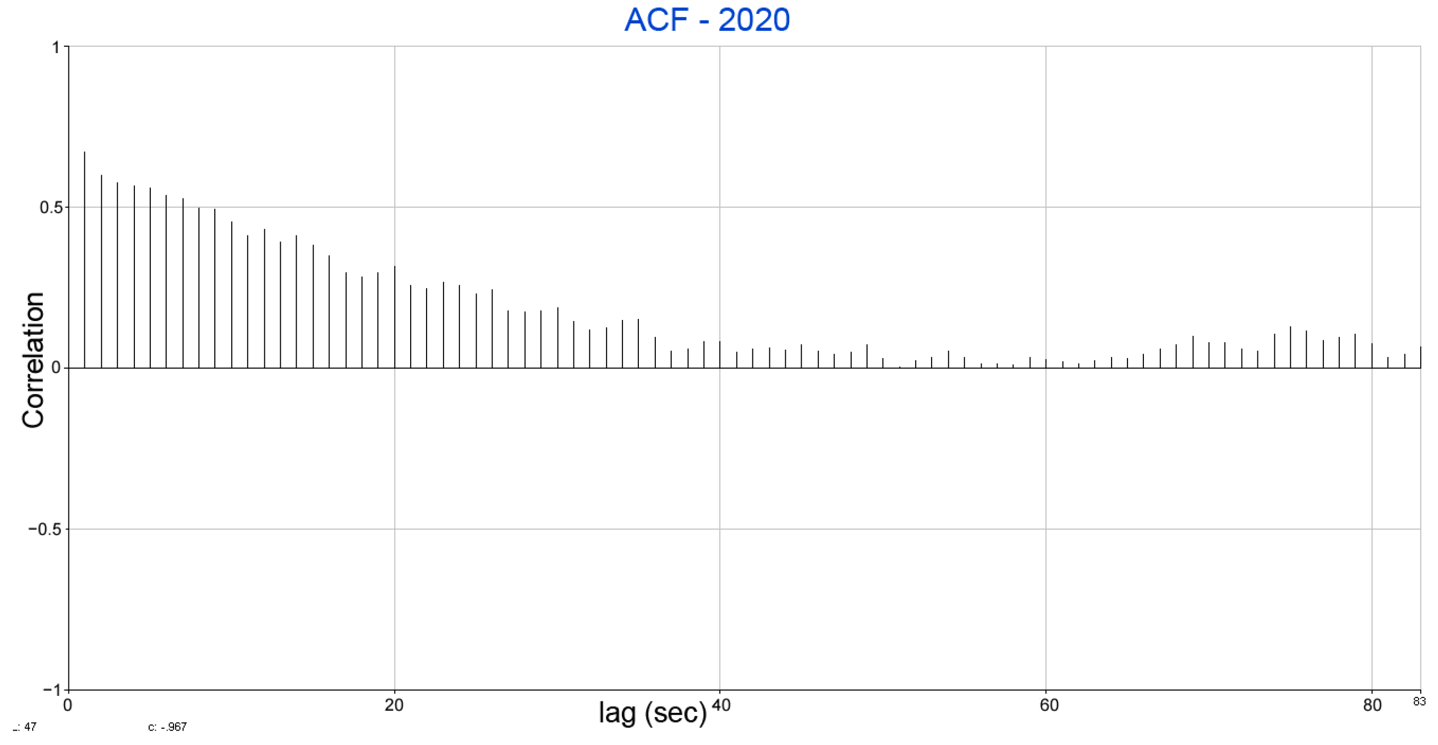
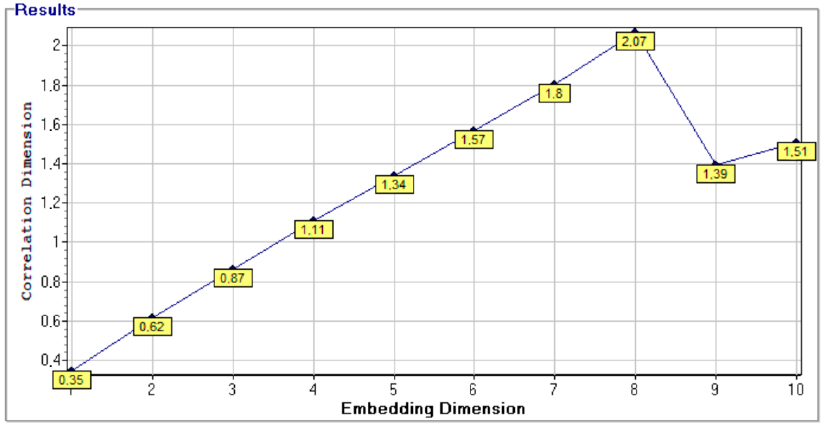
• Data of muon time series in 2020: CD = 1.613 ± 0.276
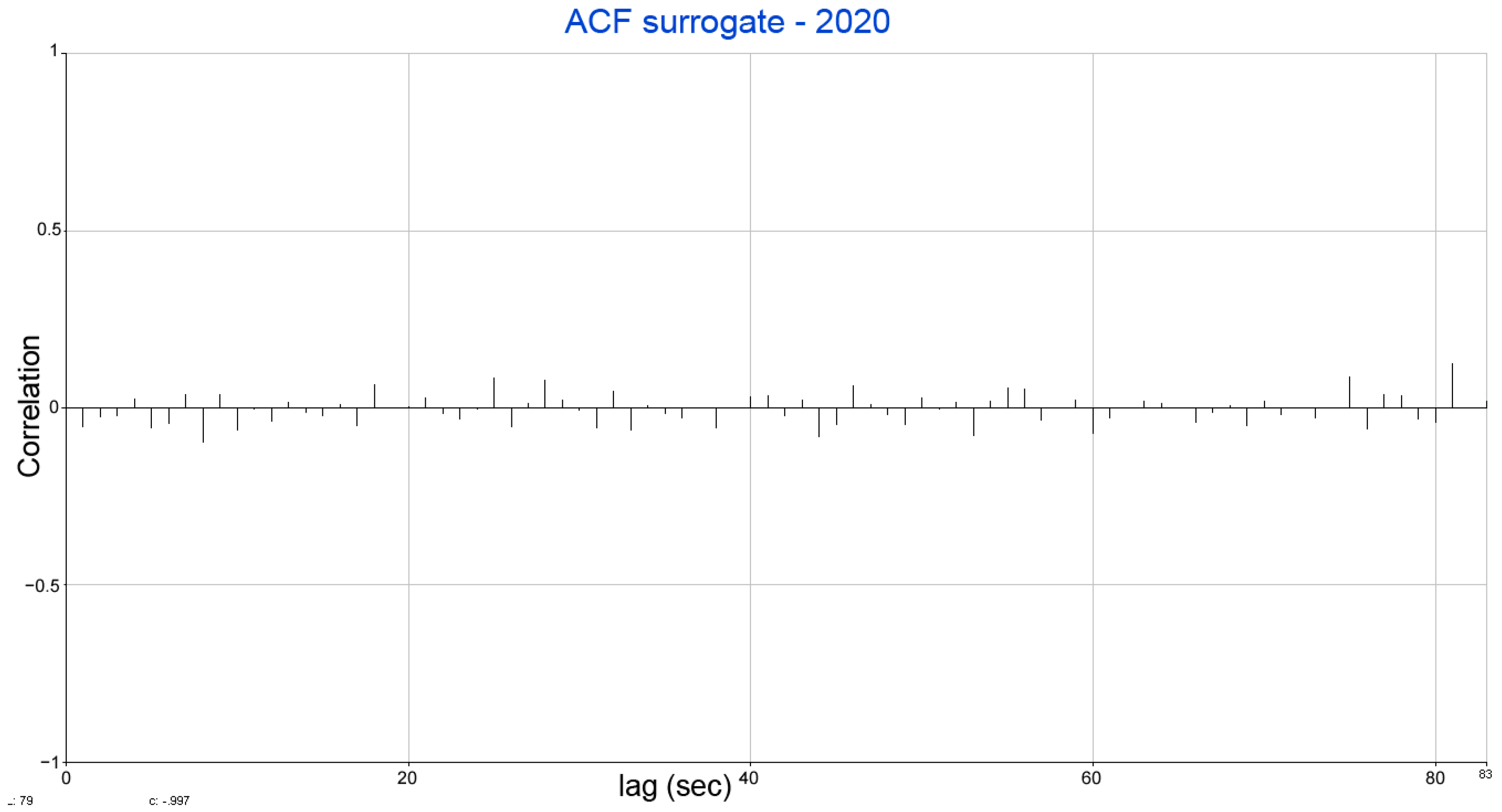
• Data of surrogate of muon time series in 2020: CD = 2.829 ± 1.183
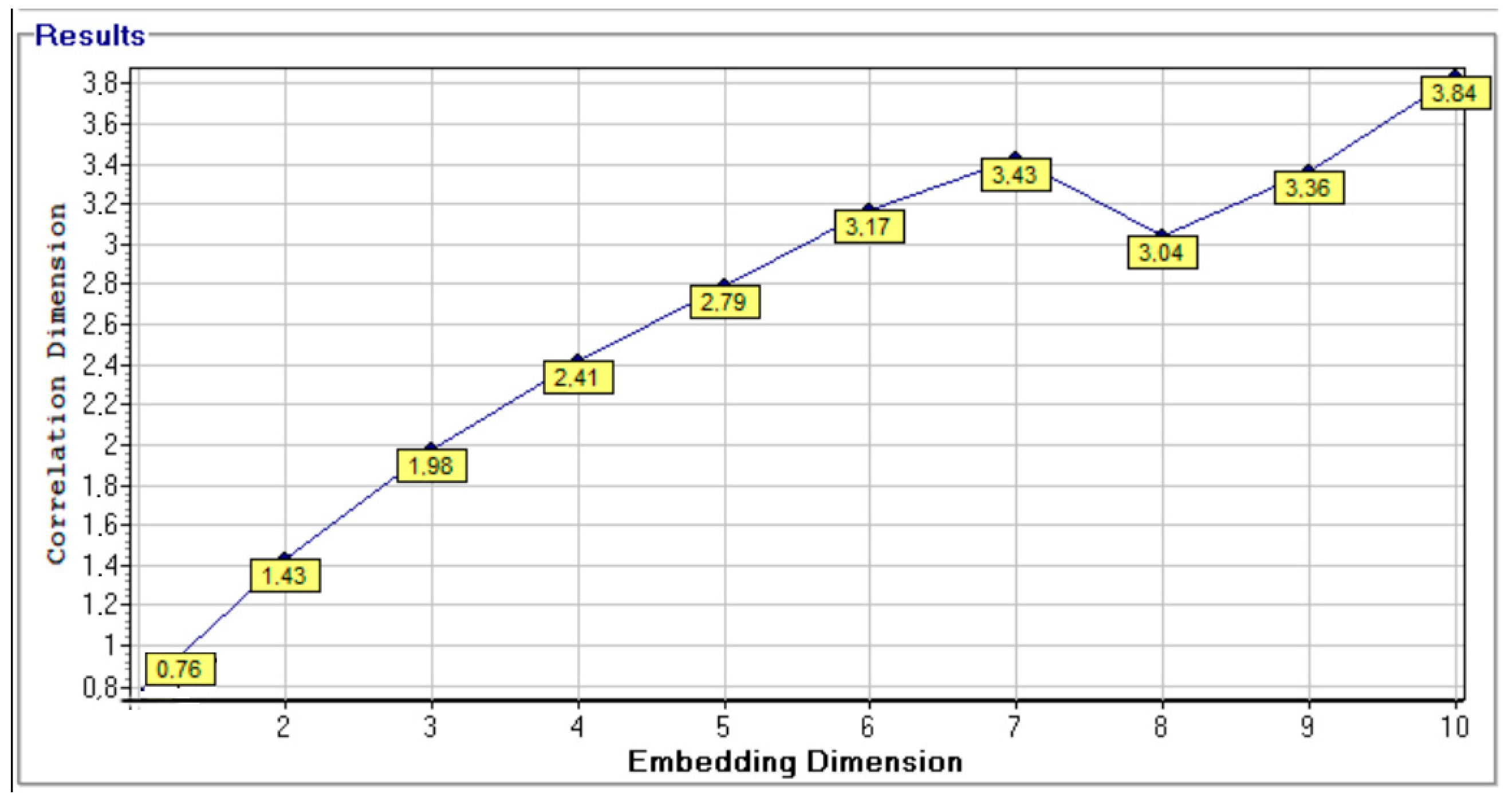
• Data of muon time series in 2021: CD = 2.621 ± 0.973
• Data of surrogate of muon time series in 2021: CD = 3.513 ± 1.620

The results indicate that the CD of muon time series runs at about the values of 1.613 and 2.621 in the years 2019, 2020 and 2021, with a value ranging from 2.736 to 3.513 for the surrogate–shuffled data. In general, the CD of surrogate data of a variable—greater than the variable itself—is a signature of chaotic dynamics. In this case, surrogate data, on average, range between 11 and 15%. In conclusion, this suggests that we are in the presence of a chaotic time series data for the recorded time series muons.

Let us now estimate the dominant Lyapunov exponent. The Lyapunov exponent, or Lyapunov characteristic exponent, or dominant Lyapunov exponent of a dynamic system, is a quantity that characterizes the rate of separation of infinitesimally close trajectories of an attractor. Quantitatively, two trajectories in phase space with initial separation vector |δZ0| diverge at a rate given by |δZ(t)| ≈ eλt |δZ0| [10,11,12], where λ is the Lyapunov exponent and is positive for a chaotic dynamical system (Figure 21).

4.3. Results of Analysis

In Figure 22a,c,e, we give the results of our analysis for the time series recorded in 2019, 2020 and 2021, and in Figure 22b,d,f, we give the results of our analysis of surrogate–shuffled data.

The results of the dominant Lyapunov exponent are 0.599 ± 0.094 for the muon time series of 2019, 0.486 ± 0.098 for the muon time series of 2020, and 0.564 ± 0.097 for the muon time series of 2021. The values of surrogate data are, respectively, 0.701 ± 0.102 for 2019, 0.657 ± 0.108 for the 2020, and, finally, of 0.790 ± 0.088 for the 2021. Such positive results of the largest Lyapunov exponent seem to indicate that we are in the presence of a chaotic dynamics.

To study the complexity of our muon time series in the years 2019, 2020, and 2021, we have also estimated the Lempel–Ziv complexity, which we will call the L–Z test. The results of such studies indicate that a measure of the algorithmic complexity of the time series is obtained.

Maximal complexity has a value near 1.0, and perfect predictability has a value of 0. In this calculation, each data point is converted to a single binary digit according to whether its value is greater than or less than the median value, and the algorithm of Kaspar and Schuster is used [12]. The results are given in Figure 23, where we see that maximum (Maximal Complexity) has been reached in 2019 with a value of 1.00275, and this is followed by satisfactory values in 2020 and 2021, with an L–Z index with the values of 0.76781 and of 0.74624, respectively.

5. Conclusions

The conclusion is that the time series recorded on muons arising from cosmic rays in the universe and measured at sea level could be of a chaotic dynamic nature. A few studies have shown chaotic features in time series of successive cosmic ray air shower arrival time intervals [15,16]. Our work shows good support for such observations, which can be backed up using small detectors. This was the only aim of the present paper. Subsequent papers will demonstrate possible correlations with atmospheric properties, such as pressure and temperature. Furthermore, the properties of the heliosphere, thus the strength of solar activity, will be taken into account, since some relationships surely could exist between the muon rate and those data. In his work, Aglietta formulated a model of such correlations [17]. Generally speaking, the muon rate, measured at sea level, depends on several mechanisms of modulation. For instance, Ohara et al. found clues suggesting some chaotic (fractal) properties, regarding a quasi-periodic behavior relating to the rotation of Earth [18]. Bergamasco et al. studied the flux of the muon series underground in search of deterministically chaotic behavior, even relating to solar activity [19]. We will start to analyze such possible correlations in subsequent papers, given the complication of such studies. To suggest the reproduction of our preliminary studies from other researchers, we note that the software we used was Chaos Data Analyzer, edited by Sprott and Rowlands, University of Wisconsin, and the Visual Recurrence Analysis, edited by Eugene Kononov.

References

1. Gamil, H.; Mehta, P.; Chielle, E.; Di Giovanni, A.; Nabeel, M.; Arneodo, F.; Maniatakos, M. Muon-Ra: Quantum Random Number Generation from Cosmic Rays. In Proceedings of the 2020 IEEE 26th International Symposium on On-Line Testing and Robust System Design (IOLTS), Napoli, Italy, 13 July 2020; pp. 1–6. [Google Scholar] [CrossRef]
2. Kumar, V.; Rayappan, J.B.B.; Amirtharajan, R.; Praveenkumar, P. Quantum True Random Number Generation on IBM’s cloud platform. J. King Saud Univ. Comput. Inf. Sci. 2022, 34, 6453–6465. [Google Scholar] [CrossRef]
3. Reitner, R.A.; Romanowski, T.; Sutton, R.; Chidley, B. Precise measurements of the mean lives of μ+ and μ mesons in carbon. Phys. Rev. Lett. 1960, 5, 22–23. [Google Scholar] [CrossRef]
4. Gutarra-Leon, A.; Barazandeh, C.; Majewski, W. Cosmic Ray Muons in the Standard Model of Fundamental Particles. Exigence 2018, 2, 1–16. [Google Scholar]
5. The Symmetry between Electrons and Muons Looks “Shaky”. Available online: https://www.uni-heidelberg.de/en/newsroom/the-symmetry-between-electrons-and-muons-looks-shaky (accessed on 1 January 2023).
6. Bothe, W.; Rossi, B. The birth and development of coincidence methods in cosmic-ray physics. Am. J. Phys. 2011, 79, 1133. [Google Scholar]
7. Arcani, M.; Conte, E.; Monte, O.D.; Frassati, A.; Grana, A.; Guaita, C.; Liguori, D.; Nemolato, A.R.M.; Pigato, D.; Rubino, E. The Astroparticle Detectors Array—An Educational Project in Cosmic Ray Physics. Symmetry 2023, 15, 294. [Google Scholar] [CrossRef]
8. Kuznetsov, N.V. The Lyapunov dimension and its estimation via the Leonov method. Phys. Lett. A 2016, 380, 2142–2149. [Google Scholar] [CrossRef] [Green Version]
9. Grassberger, P.; Procaccia, I. Measuring the Strangeness of Strange Attractors. Phys. D Nonlinear Phenom. 1983, 9, 189–208. [Google Scholar] [CrossRef]
10. Takens, F. Detecting strange attractors in turbulence. Lect. Notes Math. 1981, 898, 366–381. [Google Scholar] [CrossRef]
11. Packard, N.H.; Crutchfield, J.P.; Farmer, J.D.; Shaw, R.S. Geometry from a time series. Phys. Rev. Lett. 1980, 45, 712–716. [Google Scholar] [CrossRef]
12. Kennel, M.B.; Brown, R.; Abarbanel, H.D.I. Determining embedding dimension for phase-space reconstruction using a geometrical construction. Phys. Rev. A 1992, 45, 3403–3411. [Google Scholar] [CrossRef] [PubMed] [Green Version]
13. False Nearest Neighbor Algorithm. Available online: https://en.wikipedia.org/wiki/False_nearest_neighbor_algorithm (accessed on 1 January 2023).
14. Attractor. Available online: https://en.wikipedia.org/wiki/Attractor (accessed on 1 January 2023).
15. Ohara, S.; Konishi, T.; Mukai, A.; Shimada, M.; Iyono, A.; Matsumoto, H.; Yamamoto, I.; Takahashi, N.; Nakatsuka, T.; Okei, K.; et al. The Anisotropy of Cosmic Ray Pursued with Chaos Analysis. Int. Cosm. Ray Conf. 2011, 1, 70. [Google Scholar] [CrossRef]
16. Kitamura, T.; Ohara, S.; Konishi, T.; Tsuji, K.; Chikawa, M.; Unno, W.; Masaki, I.; Urata, K.; Kato, Y. Chaos in cosmic ray air showers. Astropart. Phys. 1997, 6, 279–291. [Google Scholar] [CrossRef]
17. Aglietta, M.; Alessandro, B.; Antonioli, P.; Arneodo, F.; Bergamasco, L.; Bertaina, M.E.; Castagnoli, C.; Castellina, A.; Chiavassa, A.; Cini, G.; et al. Search for chaotic features in the arrival times of air showers. Euro Phys. Lett. 1996, 34, 231. [Google Scholar] [CrossRef]
18. Ohara, S.; Konishi, T.; Tsuji, K.; Chikawa, M.; Kato, Y.; Wada, T.; Ochi, N.; Yamamoto, I.; Takahashi, N.; Unno, W.; et al. Chaos in different far-off cosmic rays: A fractal wave model. J. Phys. G Nucl. Part. Phys. 2003, 29, 2065. [Google Scholar] [CrossRef] [Green Version]
19. Bergamasco, L.; Serio, M.; Osborne, A.R. Correlation dimension of underground muon time series. J. Geophys. Res. 1992, 97, 17153. [Google Scholar] [CrossRef]
Figure 1. Feynman’s diagrams of muon decays.
Symmetry 15 00659 g001
Figure 2. Detector geometry response.
Symmetry 15 00659 g002
Figure 3. Raw and surrogate data of muon time series in the years (a) 2019, (b) 2020 and (c) 2021.
Symmetry 15 00659 g003
Figure 4. Probability distribution of the raw data for muon time series in the years (a) 2019, (b) 2020 and (c) 2021.
Symmetry 15 00659 g004
Figure 5. ACF of muon time series measured at sea level in 2019.
Symmetry 15 00659 g005
Figure 6. ACF on shuffled–surrogate data of muon time series measured at sea level in 2019.
Symmetry 15 00659 g006
Figure 7. ACF of muon time series measured at sea level in 2020.
Symmetry 15 00659 g007
Figure 8. ACF on shuffled–surrogate data of muon time series measured at sea level in 2020.
Symmetry 15 00659 g008
Figure 9. ACF of muon time series measured at sea level in 2021.
Symmetry 15 00659 g009
Figure 10. ACF on shuffled–surrogate data of muon time series measured at sea level in 2021.
Symmetry 15 00659 g010
Figure 11. Muon series and surrogate series: (a) AMI of the muon time series in 2019; (b) AMI of the shuffled–surrogate data of muon time series in 2019; (c) AMI of the muon time series in 2020; (d) AMI of the shuffled–surrogate data in 2020; (e) AMI of the muon time series in 2021; (f) AMI of the shuffled–surrogate data in 2021.
Symmetry 15 00659 g011
Figure 12. False nearest neighbors of data of muons in 2019.
Symmetry 15 00659 g012
Figure 13. False nearest neighbors of data of muons in 2020.
Symmetry 15 00659 g013
Figure 14. False nearest neighbors of data of muons in 2021.
Symmetry 15 00659 g014
Figure 15. Correlation dimension of muon time series in 2019.
Symmetry 15 00659 g015
Figure 16. Correlation dimension of muon time series 2020.
Symmetry 15 00659 g016
Figure 17. Correlation dimension of muon time series 2021.
Symmetry 15 00659 g017
Figure 18. The correlation dimension of surrogate–shuffled data of muon data series in 2019.
Symmetry 15 00659 g018
Figure 19. The correlation dimension of surrogate–shuffled data of muon data series in 2020.
Symmetry 15 00659 g019
Figure 20. The correlation dimension of surrogate–shuffled data of muon time series in 2021.
Symmetry 15 00659 g020
Figure 21. Rate divergence of two trajectories in phase space with initial separation|δZ0|.
Symmetry 15 00659 g021
Figure 22. Lyapunov exponent (the minimum initial separation between two data points); (a) Muon Data Series of 2019—Dominant Lyapunov exponent; (b) Surrogate–shuffled data of muon time series of 2019; (c) Muon Data Series of 2020—Dominant Lyapunov exponent; (d) Surrogate–shuffled data of muon time series of 2020; (e) Muon Data Series of 2021—Dominant Lyapunov exponent; (f) Surrogate–shuffled data of muon time series of 2021.
Symmetry 15 00659 g022
Figure 23. L–Z test of muon time series in years (a) 2019, (b) 2020, and (c) 2021.
Symmetry 15 00659 g023
Disclaimer/Publisher’s Note: The statements, opinions and data contained in all publications are solely those of the individual author(s) and contributor(s) and not of MDPI and/or the editor(s). MDPI and/or the editor(s) disclaim responsibility for any injury to people or property resulting from any ideas, methods, instructions or products referred to in the content.