Classification of Blood Rheological Models through an Idealized Symmetrical Bifurcation

Abstract

The assumed rheological behavior of blood influences the hemodynamic characteristics of numerical blood flow simulations. Until now, alternative rheological specifications have been utilized, with uncertain implications for the results obtained. This work aims to group sixteen blood rheological models in homogeneous clusters, by exploiting data generated from numerical simulations on an idealized symmetrical arterial bifurcation. Blood flow is assumed to be pulsatile and is simulated using a commercial finite volume solver. An appropriate mesh convergence study is performed, and all results are collected at three different time instants throughout the cardiac cycle: at peak systole, early diastole, and late diastole. Six hemodynamic variables are computed: the time average wall shear stress, oscillatory shear index, relative residence time, global and local non-Newtonian importance factor, and non-Newtonian effect factor. The resulting data are analyzed using hierarchical agglomerative clustering algorithms, which constitute typical unsupervised classification methods. Interestingly, the rheological models can be partitioned into three homogeneous groups, whereas three specifications appear as outliers which do not belong in any partition. Our findings suggest that models which are defined in a similar manner from a mathematical perspective may behave substantially differently in terms of the data they produce. On the other hand, models characterized by different mathematical formulations may belong to the same statistical group (cluster) and can thus be considered interchangeably.

1. Introduction

Computational fluid dynamics (CFD) have recently been employed as a powerful tool for the spatiotemporal resolution of various hemodynamics parameters, gaining considerable popularity in vascular surgery [1,2]. Especially for arterial aneurysms (either on the carotid and cerebral arteries or the aorta), rupture risk estimation and hemodynamic performance have been established as a field of continuous interest [3]. Numerical simulation of blood flow has been widely studied in the literature for various geometric configurations such as aortic arch [4,5,6], bifurcation models [7,8,9,10,11], abdominal aortic aneurysms [2,12,13,14], stenosis [15,16], and cerebral models [13,17,18,19,20].

Besides geometry, the rheological behavior of blood can significantly influence the hemodynamic output, in not only idealized but also medical-image-reconstructed computational domains. A common issue that is usually investigated is the influence of rheological models on an appropriately chosen set of hemodynamic parameters, since it is well documented that blood behaves as a non-Newtonian fluid at low shear rates. This is more prominent for values less than 100 s⁻¹ [21] and can potentially yield significant non-Newtonian effects in small vessels, or near stenoses and aneurysms [22,23,24]. The non-Newtonian nature of blood is also supported by the fact that the instantaneous shear rate throughout the cardiac cycle varies from 0 to approximately 1000 s⁻¹ [25], yielding regions of shear thinning behavior. Additionally, blood can exhibit more complex behaviors such as thixotropy or viscoelasticity. As a result, its viscosity can be altered by various parameters such as red blood cell (RBC) concentration and aggregation, hematocrit, sex, and arterial hypertension amongst others [26].

A large number of previous research studies have focused on non-Newtonian deviations in blood. The main concern is the construction of an accurate viscosity model in terms of the shear rate, yielding various candidates that have been proposed in the literature. A specific class of models that have been widely used for blood flow simulations are characterized by two asymptotic viscosity values for low and high shear rates. This class includes the Carreau (C) [5,25,27,28], Carreau–Yasuda (CY) [13,25,29,30], Cross (Cr) [15,25,31,32], Cross-modified (Cr-m) [25,31,33,34], and Cross-simplified (Cr-s) models [25,31]. This model-class is usually applied in coronary arteries [35] and has shown good agreement with experimental data [25]. Another group of blood models can be constructed in terms of shear rate and hematocrit variation. The Casson (Cs) [25,36], Casson-modified (Cs-m) [37,38], Kuang–Luo (KL) [6,31,39], Quemada (Q) [31,40,41], and Walburn–Schneck (WS) [31,42,43] models incorporate RBC volume in blood, which is expected to lie between 37% and 45%.

It has been shown that the value of hematocrit affects blood viscosity more at low shear rates than at high shear rates, enhancing non-Newtonian deviations for small shear values [44]. For the needs of this study, the hematocrit value is set equal to 40% following Cho and Kensey [25]. Another widely used blood model was introduced by Bird et al. in 1987 [45] in the form of power-law (P) [38,39,43,46]. Even though the model accurately mimics blood for high shear rates, it fails in both low and high shear rate regions as pointed out in [6]. An extended version of the power-law model that is capable of achieving this, is the so-called generalized power-law (P-g) [5,6], mainly due to the large number of parameters involved. Additional models such as the Herschel–Bulkley (HB) [2,47], Powell–Eyring (PE) [25,48], and Powell–Eyring modified (PE-m) [25] form an almost complete set of candidates for the description of blood under a wide range of physiological conditions.

An investigation of the literature suggests that different rheological models are used interchangeably during computational modeling, with uncertain implications for the results obtained. Therefore, this work aims to group alternative specifications into homogeneous clusters; data generated from models in different clusters should be viewed as significantly different. A priori, the aforementioned non-Newtonian specifications can be divided into four main partitions, based on their underlying mathematical formulation. Specifically, the first initial partition, dubbed IP1, contains C, CY, Cr, Cr-m, and Cr-s; IP2 consists of Cs, Cs-m, KL, Q, and WS; the power-law-based (P and P-g) and Powell–Eyring-based (PE and PE-m) variants constitute IP3 and IP4, respectively. Alternatively, each rheological specification can be viewed as a data-generating process; hence, model grouping can be based on a statistical unsupervised classification procedure, applied to the simulated explanatory variables that characterize each model. To our knowledge, this is the first study that classifies alternative rheologies using statistical clustering techniques. It is of interest to evaluate the derived groups that coincide with the a priori partitions. Furthermore, statistical analysis is expected to reveal (a) homogeneous groups, or clusters of specifications, which are close in terms of their distances in the multi-dimensional space spanned by the simulated explanatory variables; (b) models that can be viewed as representatives of each cluster; (c) outlying specifications which do not belong in any cluster; and (d) hemodynamic variables that characterize each cluster.

The manuscript is organized as follows: Section 2 describes the mathematical framework that is adopted for the numerical simulation of non-Newtonian fluid flow; furthermore, it formulates the assumed rheological models and discusses the statistical methodology. Section 3 presents the results of the clustering procedure. Section 4 elucidates the statistical and hemodynamic outcomes of this work, and Section 5 contains the concluding remarks. Finally, all relevant data analyzed herein are provided to the interested reader as supplementary information.

2. Materials and Methods

2.1. Governing Equations and Simulation Setup

Blood is modelled as a homogeneous, incompressible, and non-Newtonian fluid. All simulations are performed by solving the three-dimensional Navier–Stokes and continuity equations

$$\begin{array}{c}\mathsf{\rho }\left[\frac{\partial \mathbf{U}}{\partial \mathrm{t}}+(\mathbf{U}·\nabla )\mathbf{U}\right]=-\nabla \mathrm{p}+\nabla ·\mathsf{\tau },\\ \nabla ·\mathbf{U}=0,\end{array}$$

where $\mathbf{U},\hspace{0.33em}\mathrm{p},\hspace{0.33em}\mathsf{\rho }$ represent the fluid velocity, pressure, and density respectively. For the non-Newtonian fluids considered here, the stress tensor depends linearly on the rate-of-deformation tensor $\mathbf{D}=\left[\nabla \mathbf{U}+{\left(\nabla \mathbf{U}\right)}^{\mathrm{T}}\right]/2;$ that is

$$\mathsf{\tau }=2\hspace{0.17em}\mathsf{\mu }\left(\dot{\mathsf{\gamma }}\right)\hspace{0.17em}\mathbf{D}.$$

Furthermore, the shear rate dependent viscosity of blood is determined by the second invariant of the rate-of-deformation tensor, since

$$\dot{\mathsf{\gamma }}=\sqrt{\frac{1}{2}\hspace{0.17em}\mathbf{D}\otimes \mathbf{D}}.$$

Vascular flows can then be analyzed in terms of the near wall hemodynamic parameters over the entire cardiac cycle, T, such as the wall shear stress (WSS) and its most commonly used metrics, the time average wall shear stress (TAWSS, Pa), oscillatory shear index (OSI), and relative residence time (RRT, Pa⁻¹). Let WSS represent the WSS vector, defined as the dot product of the outward unit normal vector on a surface with the stress tensor; then, TAWSS is expressed as follows

$$\mathrm{T}\mathrm{A}\mathrm{W}\mathrm{S}\mathrm{S}=\frac{1}{\mathrm{T}}{{\displaystyle \int }}_0^{\mathrm{T}}\left|\mathbf{W}\mathbf{S}\mathbf{S}\right|\mathrm{d}\mathrm{t}.$$

Even though TAWSS quantifies the tangential force on the vessel wall due to blood flow as the average magnitude of the shear stress, it does not provide any information on the varying frequency of the WSS direction. To describe the oscillatory nature of flows, the work in [49] introduced the non-dimensional OSI, which is formulated as

$$\mathrm{O}\mathrm{S}\mathrm{I}=\frac{1}{2}\left(1-\frac{\mid {{\displaystyle \int }}_0^{\mathrm{T}} \mathbf{W}\mathbf{S}\mathbf{S} \mathrm{d}\mathrm{t}\mid }{{{\displaystyle \int }}_0^{\mathrm{T}}\mid \mathbf{W}\mathbf{S}\mathbf{S}\mid \mathrm{d}\mathrm{t}}\right),$$

with $0\le \mathrm{O}\mathrm{S}\mathrm{I}\le 0.5.$ Flows characterized by no cyclic variation in WSS, such as uniaxial flows, correspond to $\mathrm{O}\mathrm{S}\mathrm{I}=0,$ while flows with no preferred direction, where the time average of the instantaneous WSS vanishes, yield $\mathrm{O}\mathrm{S}\mathrm{I}=0.5.$ Finally, Himburg et al. [50] introduced RRT in terms of the two previous hemodynamic markers as

$$\mathrm{R}\mathrm{R}\mathrm{T}=\frac{1}{\left(1-2·\mathrm{O}\mathrm{S}\mathrm{I}\right)·\mathrm{T}\mathrm{A}\mathrm{W}\mathrm{S}\mathrm{S}}.$$

RRT identifies regions of high particle residence time inside the fluid domain. It is worth noting that the abovementioned metrics have been associated with various diseased states, such as thrombogenic stimulating environments for TAWSS < 0.4 Pa [51], OSI > 0.3 [50], and RRT > 10 Pa⁻¹ [52].

An additional set of variables that characterize the non-Newtonian deviation of fluid flows are (a) the local non-Newtonian importance factor I_L [53]; (b) the global non-Newtonian importance factor I_G [53]; and (c) the non-Newtonian effect factor NNEF [54]. These variables compare the physical quantities of non-Newtonian rheological models with respect to their Newtonian counterparts and are defined as

$$\begin{array}{l}{\mathrm{I}}_{\mathrm{L}}=\frac{\mathsf{\mu }}{{\mathsf{\mu }}_{\infty }},\\ {\mathrm{I}}_{\mathrm{G}}=\frac{1}{\mathrm{N}}\frac{{\left[{\displaystyle \sum _{\mathrm{N}}{\left(\mathsf{\mu }-{\mathsf{\mu }}_{\infty }\right)}^2}\right]}^{1/2}}{{\mathsf{\mu }}_{\infty }}·100,\\ \mathrm{N}\mathrm{N}\mathrm{E}\mathrm{F}=\frac{{\left(\mathrm{W}\mathrm{S}\mathrm{S}\right)}_{\mathrm{n}\mathrm{o}\mathrm{n}-\mathrm{N}\mathrm{e}\mathrm{w}\mathrm{t}\mathrm{o}\mathrm{n}\mathrm{i}\mathrm{a}\mathrm{n}}-{\left(\mathrm{W}\mathrm{S}\mathrm{S}\right)}_{\mathrm{N}\mathrm{e}\mathrm{w}\mathrm{t}\mathrm{o}\mathrm{n}\mathrm{i}\mathrm{a}\mathrm{n}}}{{\left(\mathrm{W}\mathrm{S}\mathrm{S}\right)}_{\mathrm{N}\mathrm{e}\mathrm{w}\mathrm{t}\mathrm{o}\mathrm{n}\mathrm{i}\mathrm{a}\mathrm{n}}}.\end{array}$$

In the above definitions, ${\mathsf{\mu }}_{\infty },$ is the viscosity of the Newtonian model (equal to $0.00345\hspace{0.33em}\mathrm{P}\mathrm{a}·\mathrm{s}$ in this study), and the summation is performed over all N grid nodes that constitute the wall or fluid of the computational domain. The trivial case of $\left({\mathrm{I}}_{\mathrm{L}},\hspace{0.33em}{\mathrm{I}}_{\mathrm{G}},\hspace{0.33em}\mathrm{N}\mathrm{N}\mathrm{E}\mathrm{F}\right)=\left(1,\hspace{0.33em}0,\hspace{0.33em}0\right)$ corresponds to the Newtonian case.

A commercial finite volume solver is utilized (Fluent 17.2, ANSYS Inc.) for all numerical simulations herein. The SIMPLEC algorithm is adopted for pressure–velocity coupling and the default criterion for solution convergence is set to 10⁻⁴. In addition, the time step is kept constant (equal to 0.005 s), and four flow cycles are simulated before results are collected in order to ensure that all transient effects are washed out. This is achieved by ensuring that the velocity magnitude at the outlets does not vary more than 0.5% between successive cardiac cycles. In all cases, a rigid wall is assumed with a no-slip boundary condition at the wall boundary. Transient velocity and pressure waveforms are prescribed at the inlet and outlets respectively for a cycle of one second. Both waveforms (Figure 1) closely follow Olufsen et al. [55]. The corresponding profiles are prescribed using appropriate user-defined functions (UDFs), and the Womersley method is applied for the inlet velocity, with a constant Womersley parameter equal to 17.97. The analyzed data are collected at peak systole (t = 0.23 s), early (t = 0.46 s), and late diastole (t = 0.8 s).

2.2. Non-Newtonian Blood Rheological Models

Table 1. Rheological models examined in this study. All quantities are expressed in SI units unless otherwise stated.

#	Name (Abbreviation)	Equation	Parameter Values	References
1	Carreau (C)	$\mathsf{\mu }\left(\dot{\mathsf{\gamma }}\right)={\mathsf{\mu }}_{\infty }+\frac{\left({\mathsf{\mu }}_0-{\mathsf{\mu }}_{\infty }\right)}{{\left[1+{\left(\lambda \dot{\mathsf{\gamma }}\right)}^2\right]}^{\left(1-\mathrm{n}\right)/2}}$	$\begin{array}{l}{\mathsf{\mu }}_{\infty }=0.00345,\hspace{0.33em}{\mathsf{\mu }}_0=0.056\\ \hspace{0.33em}\hspace{0.33em}\hspace{0.33em}\lambda =3.313,\hspace{0.33em}\mathrm{n}=0.3568\end{array}$	[5,25,27,28]
2	Carreau–Yasuda (CY)	$\mathsf{\mu }\left(\dot{\mathsf{\gamma }}\right)={\mathsf{\mu }}_{\infty }+\frac{\left({\mathsf{\mu }}_0-{\mathsf{\mu }}_{\infty }\right)}{\left[1+{\left(\lambda \dot{\mathsf{\gamma }}\right)}^{\mathsf{\alpha }}\right]{\hspace{0.17em}}^{\left(1\hspace{0.17em}-\hspace{0.17em}\mathrm{n}\right)/\mathsf{\alpha }}}$	$\begin{array}{l}\hspace{0.33em}\hspace{0.33em}{\mathsf{\mu }}_{\infty }=0.00345,\hspace{0.33em}{\mathsf{\mu }}_0=0.056\\ \lambda =1.902,\hspace{0.33em}\mathrm{n}=0.22,\hspace{0.33em}\mathsf{\alpha }=1.25\end{array}$	[13,25,29,30]
3	Casson (Cs)	$\mathsf{\mu }\left(\dot{\mathsf{\gamma }}\right)={\left(\sqrt{\hspace{0.17em}\mathrm{k}}+\frac{\sqrt{\hspace{0.17em}{\mathsf{\tau }}_0}}{\sqrt{\hspace{0.17em}\dot{\mathsf{\gamma }}}}\right)}^2$	$\mathrm{k}=0.00345,\hspace{0.33em}{\mathsf{\tau }}_0=0.005$	[25,36]
4	Casson modified (Cs-m)	$\mathsf{\mu }\left(\dot{\mathsf{\gamma }}\right)={\left(\sqrt{\hspace{0.17em}\mathrm{k}}+\frac{\sqrt{\hspace{0.17em}{\mathsf{\tau }}_0}}{\sqrt{\hspace{0.17em}\dot{\mathsf{\gamma }}}+\sqrt{\hspace{0.17em}\lambda }}\right)}^2$	$\begin{array}{l}\hspace{1em}\hspace{0.33em}\hspace{0.33em}\mathrm{k}=0.00345,\hspace{0.33em}\\ {\mathsf{\tau }}_0=0.021,\hspace{0.33em}\lambda =11.5\end{array}$	[37,38]
5	Cross (Cr)	$\mathsf{\mu }\left(\dot{\mathsf{\gamma }}\right)={\mathsf{\mu }}_{\infty }+\frac{\left({\mathsf{\mu }}_0-{\mathsf{\mu }}_{\infty }\right)}{1+{\left(\lambda \dot{\mathsf{\gamma }}\right)}^{\mathrm{m}}}$	$\begin{array}{l}{\mathsf{\mu }}_{\infty }=0.00345,\hspace{0.33em}{\mathsf{\mu }}_0=0.056\\ \hspace{0.33em}\hspace{0.33em}\hspace{0.33em}\lambda =1.007,\hspace{0.33em}\mathrm{m}=1.028\end{array}$	[15,25,31,32]
6	Cross modified (Cr-m)	$\mathsf{\mu }\left(\dot{\mathsf{\gamma }}\right)={\mathsf{\mu }}_{\infty }+\frac{\left({\mathsf{\mu }}_0-{\mathsf{\mu }}_{\infty }\right)}{{\left[1+{\left(\lambda \dot{\mathsf{\gamma }}\right)}^{\mathrm{m}}\right]}^{\hspace{0.17em}\mathsf{\alpha }}}$	$\begin{array}{l}\hspace{0.33em}\hspace{0.33em}{\mathsf{\mu }}_{\infty }=0.0035,\hspace{0.33em}{\mathsf{\mu }}_0=0.16\\ \lambda =8.2,\hspace{0.33em}\mathrm{m}=0.64,\hspace{0.33em}\mathsf{\alpha }=1.23\end{array}$	[25,31,33,34]
7	Cross simplified (Cr-s)	$\mathsf{\mu }\left(\dot{\mathsf{\gamma }}\right)={\mathsf{\mu }}_{\infty }+\frac{\left({\mathsf{\mu }}_0-{\mathsf{\mu }}_{\infty }\right)}{1+\lambda \dot{\mathsf{\gamma }}}$	${\mathsf{\mu }}_{\infty }=0.005,\hspace{0.33em}{\mathsf{\mu }}_0=0.13,\hspace{0.33em}\lambda =8$	[25,31]
8	Herschel–Bulkley (HB)	$\mathsf{\mu }\left(\dot{\mathsf{\gamma }}\right)=\mathrm{k}\hspace{0.17em}{\dot{\mathsf{\gamma }}}^{\mathrm{n}-1}+\frac{{\mathsf{\tau }}_0\left(1-{\mathrm{e}}^{-\mathrm{m}\hspace{0.17em}\dot{\mathsf{\gamma }}}\right)}{\dot{\mathsf{\gamma }}}$	$\begin{array}{l}{\mathsf{\tau }}_0=0.00345,\hspace{0.33em}\mathrm{k}=0.008\\ \hspace{0.33em}\hspace{0.33em}\mathrm{n}=0.8375,\hspace{0.33em}\mathrm{m}=1000\end{array}$	[2,47]
9	Kuang–Luo (KL)	$\mathsf{\mu }\left(\dot{\mathsf{\gamma }}\right)=\frac{1}{\dot{\mathsf{\gamma }}}\hspace{0.17em}\hspace{0.17em}\left[{\tau }_0+{\mathsf{\mu }}_{\mathrm{c}}\left({\mathsf{\alpha }}_2\sqrt{\dot{\mathsf{\gamma }}}+{\mathsf{\alpha }}_1\hspace{0.17em}\dot{\mathsf{\gamma }}\right)\right]$	$\begin{array}{l}{\tau }_0=0.005,\hspace{0.33em}{\mathsf{\mu }}_{\mathrm{c}}=0.0035,\\ \hspace{0.33em}{\mathsf{\alpha }}_1=1.0,\hspace{0.33em}{\mathsf{\alpha }}_2=1.19523\end{array}$	[6,31,39]
10	Newtonian (N)	$\mathsf{\mu }\left(\dot{\mathsf{\gamma }}\right)={\mathsf{\mu }}_{\infty }$	${\mathsf{\mu }}_{\infty }=0.00345$	[42,56]
11	Powell–Eyring (PE)	$\mathsf{\mu }\left(\dot{\mathsf{\gamma }}\right)={\mathsf{\mu }}_{\infty }+\left({\mathsf{\mu }}_0-{\mathsf{\mu }}_{\infty }\right)\frac{{\sinh }^{-1}\left(\lambda \dot{\mathsf{\gamma }}\right)}{\lambda \dot{\mathsf{\gamma }}}$	$\begin{array}{l}{\mathsf{\mu }}_{\infty }=0.00345,\hspace{0.33em}{\mathsf{\mu }}_0=0.056\\ \hspace{1em}\hspace{1em}\hspace{1em}\lambda =5.383\end{array}$	[25,48]
12	Powell–Eyring modified (PE-m)	$\mathsf{\mu }\left(\dot{\mathsf{\gamma }}\right)={\mathsf{\mu }}_{\infty }+\left({\mathsf{\mu }}_0-{\mathsf{\mu }}_{\infty }\right)\frac{\ln \left(\lambda \dot{\mathsf{\gamma }}+1\right)}{{\left(\lambda \dot{\mathsf{\gamma }}\right)}^{\mathrm{m}}}$	$\begin{array}{l}{\mathsf{\mu }}_{\infty }=0.00345,\hspace{0.33em}{\mathsf{\mu }}_0=0.056\\ \hspace{0.33em}\hspace{0.33em}\hspace{0.33em}\hspace{0.33em}\lambda =2.415,\hspace{0.33em}\mathrm{m}=1.089\end{array}$	[25]
13	Power-law (P)	$\mathsf{\mu }\left(\dot{\mathsf{\gamma }}\right)=\mathrm{k}\hspace{0.17em}{\dot{\mathsf{\gamma }}}^{\mathrm{n}-1}$	$\mathrm{k}=0.01467,\hspace{0.33em}\mathrm{n}=0.7755$	[38,39,43,45,46]
14	Power-law generalized (P-g)	$\begin{array}{l}\hspace{1em}\hspace{1em}\hspace{1em}\hspace{1em}\hspace{1em}\mathsf{\mu }\left(\dot{\mathsf{\gamma }}\right)=\mathrm{k}\left(\dot{\mathsf{\gamma }}\right)\hspace{0.17em}{\dot{\mathsf{\gamma }}}^{\mathrm{n}\left(\dot{\mathsf{\gamma }}\right)-1}\\ \mathrm{k}\left(\dot{\mathsf{\gamma }}\right)={\mathsf{\mu }}_{\infty }+\Delta \mathsf{\mu }\hspace{0.33em}\mathrm{e}\mathrm{x}\mathrm{p}\left[-\left(1+\frac{\dot{\mathsf{\gamma }}}{\mathsf{\alpha }}\right)\mathrm{e}\mathrm{x}\mathrm{p}\left(-\frac{\mathrm{b}}{\dot{\mathsf{\gamma }}}\right)\right]\\ \mathrm{n}\left(\dot{\mathsf{\gamma }}\right)={\mathrm{n}}_{\infty }+\Delta \mathrm{n}\hspace{0.33em}\mathrm{e}\mathrm{x}\mathrm{p}\left[-\left(1+\frac{\dot{\mathsf{\gamma }}}{\mathrm{c}}\right)\mathrm{e}\mathrm{x}\mathrm{p}\left(-\frac{\mathrm{d}}{\dot{\mathsf{\gamma }}}\right)\right]\end{array}$	$\begin{array}{l}{\mathsf{\mu }}_{\infty }=0.0035,\hspace{0.33em}\Delta \mathsf{\mu }=0.025,\hspace{0.33em}\\ \hspace{1em}\hspace{1em}\hspace{0.33em}\mathsf{\alpha }=50,\hspace{0.33em}\mathrm{b}=3,\\ \hspace{1em}{\mathrm{n}}_{\infty }=1.0,\hspace{0.33em}\Delta \mathrm{n}=0.45,\hspace{0.33em}\\ \hspace{1em}\hspace{1em}\hspace{0.33em}\mathrm{c}=50,\hspace{0.33em}\mathrm{d}=4\end{array}$	[5,6]
15	Quemada (Q)	$\mathsf{\mu }\left(\dot{\mathsf{\gamma }}\right)={\mathsf{\mu }}_0{\left(1-\frac{1}{2}\frac{{\mathrm{k}}_0+{\mathrm{k}}_{\infty }\sqrt{\left|\dot{\mathsf{\gamma }}\right|/{\mathsf{\gamma }}_{\mathrm{c}}}}{1+\sqrt{\left|\dot{\mathsf{\gamma }}\right|/{\mathsf{\gamma }}_{\mathrm{c}}}}\mathsf{\varphi }\right)}^{-2}$	$\begin{array}{l}\hspace{1em}{\mathsf{\mu }}_0=0.0012,\hspace{0.33em}{\mathsf{\gamma }}_{\mathrm{c}}=1.88\\ {\mathrm{k}}_0=4.33,\hspace{0.33em}{\mathrm{k}}_{\infty }=2.07,\hspace{0.33em}\mathsf{\varphi }=0.4\end{array}$	[31,40,41]
16	Walburn–Schneck (WS)	$\mathsf{\mu }\left(\dot{\mathsf{\gamma }}\right)={\mathrm{C}}_1\hspace{0.17em}{\mathrm{e}}^{\hspace{0.17em}{\mathrm{C}}_2\hspace{0.17em}\mathrm{H}}\hspace{0.17em}{\mathrm{e}}^{\hspace{0.17em}{\mathrm{C}}_4\hspace{0.17em}\mathrm{T}\mathrm{P}\mathrm{M}\mathrm{A}/{\mathrm{H}}^2}\hspace{0.17em}{\dot{\mathsf{\gamma }}}^{-{\mathrm{C}}_3\mathrm{H}}$	$\begin{array}{l}\hspace{0.33em}\hspace{0.33em}{\mathrm{C}}_1=0.000797,\hspace{0.33em}{\mathrm{C}}_2=0.0608,\\ {\mathrm{C}}_3=0.00499,\hspace{0.33em}{\mathrm{C}}_4=14.585\hspace{0.33em}\mathrm{L}/\mathrm{g},\\ \hspace{0.33em}\hspace{0.33em}\hspace{0.33em}\mathrm{T}\mathrm{P}\mathrm{M}\mathrm{A}=25.9\hspace{0.33em}\mathrm{g}/\mathrm{L},\hspace{0.33em}\mathrm{H}=40\end{array}$	[31,42,43]

presents (in alphabetical order) the 16 rheological models for blood that are analyzed herein; the table also presents typical parameter values and representative references. A graphical illustration is shown on Figure 2; one clearly observes that for shear rate values greater than 100 s⁻¹, all specifications converge to the Newtonian case.

2.3. Grid Generation and Mesh Convergence

The geometry of the model is built using SolidWorks (Dassault Systèmes). Specifically, the inlet and outlet diameters are set equal to $\mathrm{D}=26\hspace{0.33em}\mathrm{m}\mathrm{m}$ and $\mathrm{d}=12\hspace{0.33em}\mathrm{m}\mathrm{m}$, respectively. The angle between limbs is set to $\mathsf{\phi }={40}^{\circ }$, and a mild fillet of $1\hspace{0.33em}\mathrm{m}\mathrm{m}$ is considered at the bifurcation area to avoid sharp edges. Finally, the length of the parent and daughter vessels are set to $\mathrm{y}=80\hspace{0.33em}\mathrm{m}\mathrm{m}$ and $\mathrm{x}=140\hspace{0.33em}\mathrm{m}\mathrm{m}$, respectively. The selected geometry aims to approximate realistic anatomic configurations of the infrarenal abdominal aorta and the aortic bifurcation, so that our conclusions are clinically relevant. In this regard, not only does the selected geometry fall well within the normal range of infrarenal aortic anatomy, but it is also representative of the typical dimensions of standard endoluminal grafts that are used during standard endovascular treatment of aortic occlusive or aneurysmal disease [57]. The solid model is meshed with ANSA (BETA CAE Systems S.A.) using a pure hexahedral mesh; such meshes are preferred to tetrahedral or prismatic ones as they require fewer elements for a fixed level of accuracy [58]. Figure 3 presents the key features of the adopted configuration.

A mesh convergence analysis is performed next; to this end, four different meshes are adopted (

Table 2. Details of the four meshes assumed for mesh convergence. The table presents the total number of elements and nodes, as well as the number of boundary layer (BL) element levels and minimum element size on the boundary layer.

Mesh	# of Elements	# of Nodes	BL Levels	BL Min (mm)
Coarse	282450	299194	5	0.2688
Medium	660000	683789	10	0.0770
Fine	1229952	1263617	14	0.0338
Extra fine	2464640	2515452	19	0.0129

). In all cases, the boundary layer (BL) occupies approximately 10% of the inlet radius, and each level is constructed with a geometric factor of 1.2 with respect to the previous one. Four different physical quantities are considered for mesh convergence: TAWSS, OSI, average outlet velocity, and volume pressure integral. The specific choice of quantities is made in order to account for a wide range of model components such as wall, outlet, and fluid. A 1% error threshold is assumed for mesh convergence; the corresponding results are presented in

Table 3. Results and percentage errors for TAWSS, OSI, average outlet velocity, and volume pressure integral. All errors are calculated with respect to the extra fine mesh.

Mesh	TAWSS Result (Pa)/Error (%)		OSI Result/Error (%)		Outlet Velocity Result (m/s)/Error (%)		Volume Pressure Integral Result (Pa·m3)/Error (%)
Coarse	0.7905	6.65%	0.2117	5.96%	0.0548	2.81%	1.4225	−6.44%
Medium	0.7623	2.85%	0.2043	2.25%	0.0541	1.50%	1.4578	−4.12%
Fine	0.7433	0.28%	0.2010	0.60%	0.0535	0.38%	1.5312	−0.70%
Extra fine	0.7412	-	0.1998	-	0.0533	-	1.5205	-

. Thus, all simulations are performed with the so-called fine mesh.

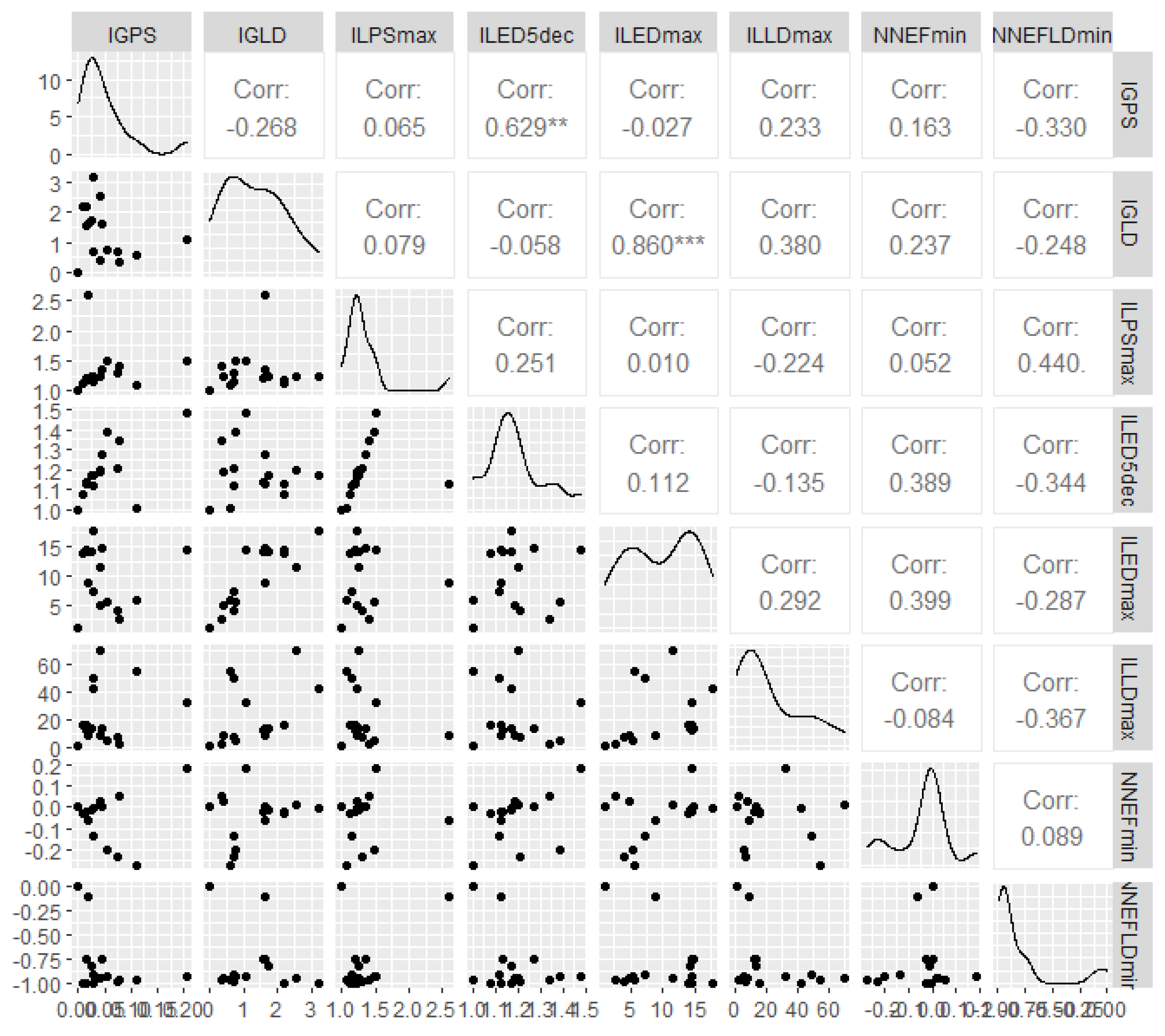
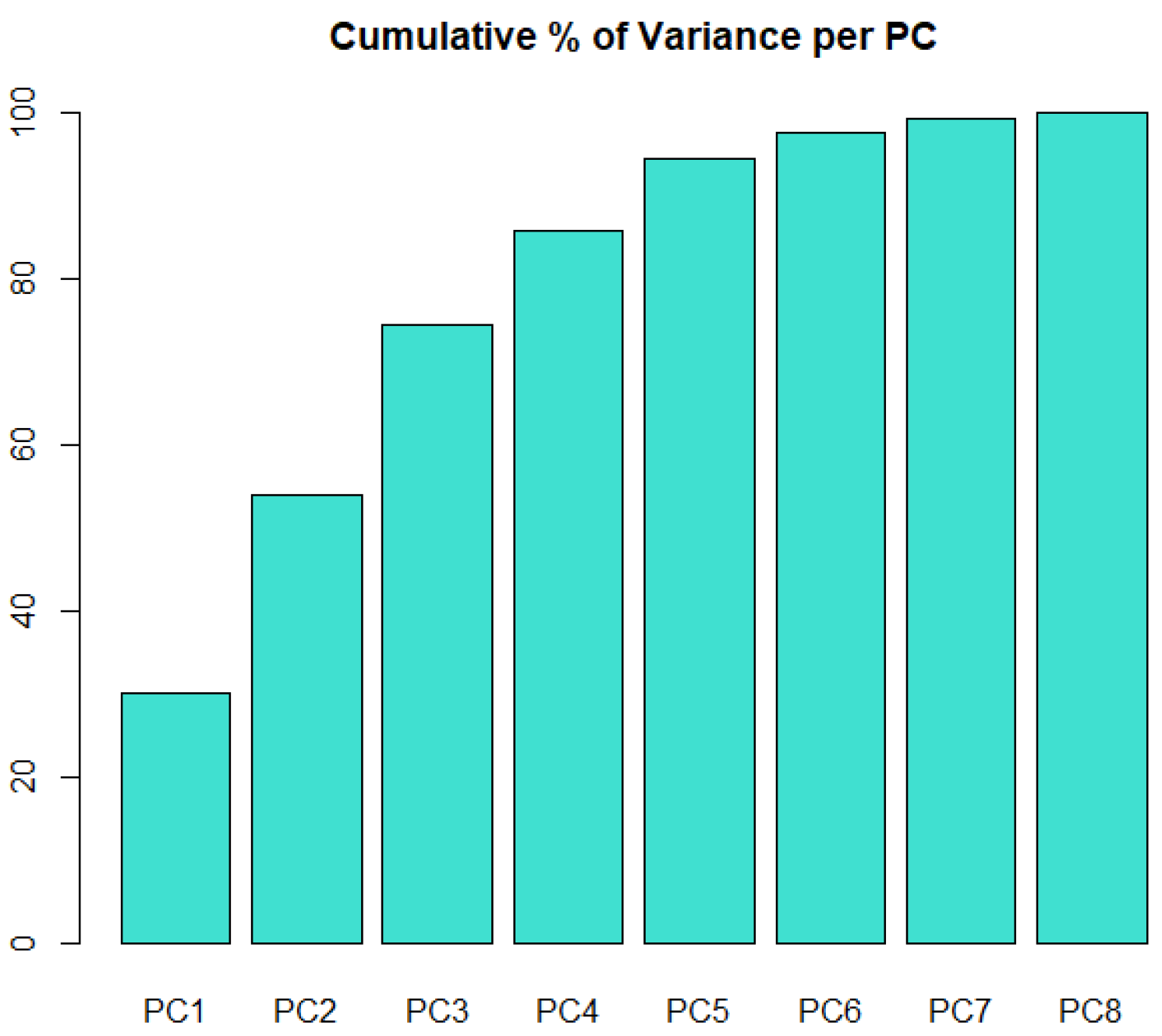
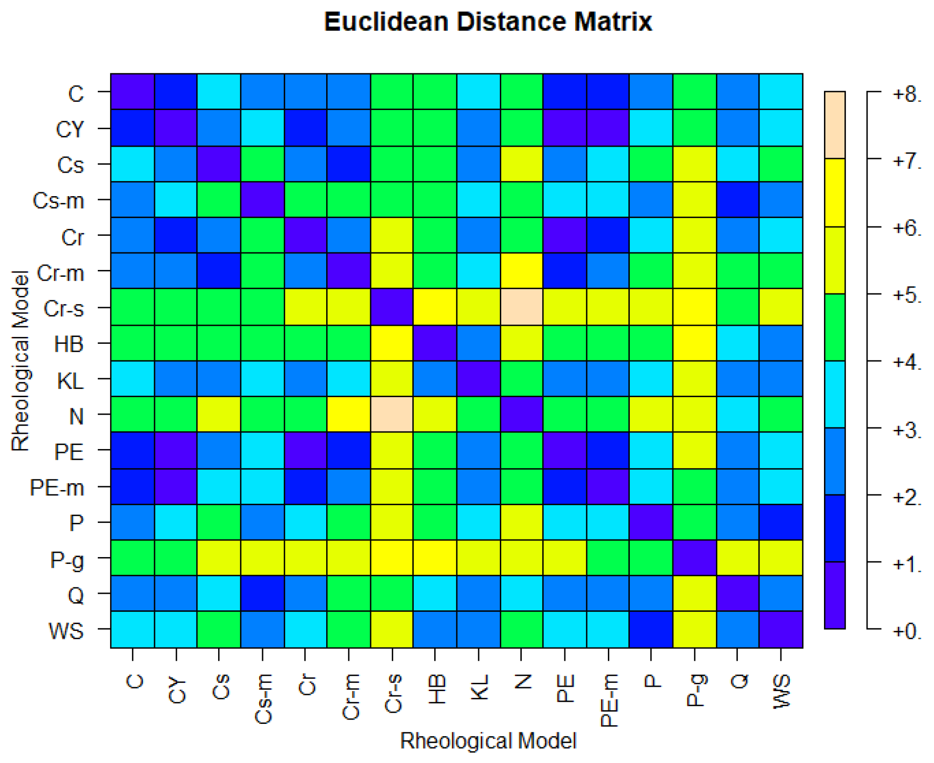
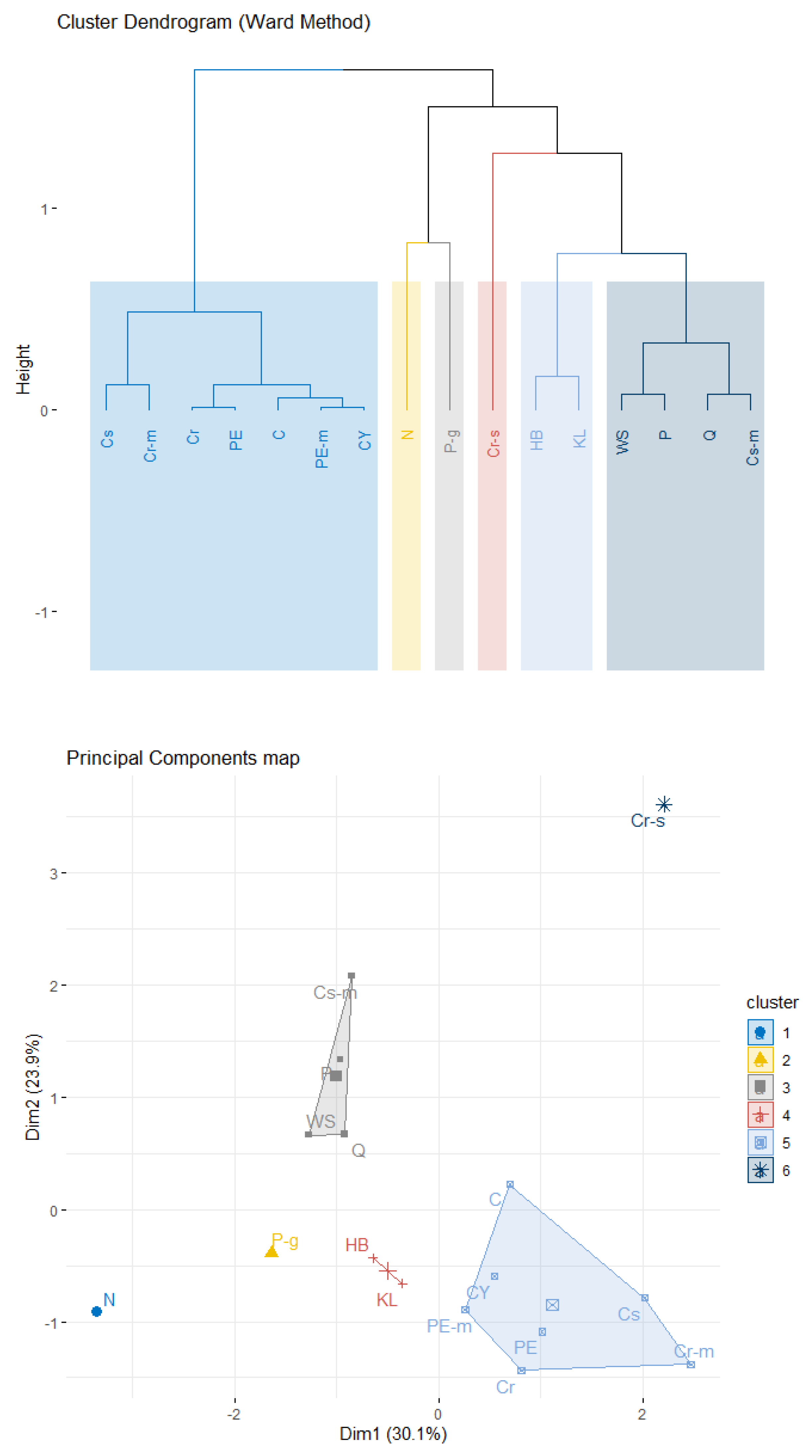
2.4. Statistical Analysis

Dimensionality reduction via correlation-based filtering of explanatory variables constitutes the first stage of the statistical analysis. The necessity of this procedure stems from the high-dimensional data generated by simulation: the total number of explanatory variables that characterize each rheological model is much larger than the number of examined models. The analysis of unfiltered, multi-collinear, high-dimensional data is not straightforward for standard multivariate statistical procedures and may lead to inefficient estimators that are not accurate in small samples [59]. Hence, redundant information is eliminated via variance-inflation filtering; a stepwise procedure dubbed VIFstep eliminates a predictor if it can be derived as a linear combination of other predictors [60].

Specifically, for the ith predictor, the variance inflation criterion is expressed as

$$\mathrm{V}\mathrm{I}{\mathrm{F}}_{\mathrm{I}}=\frac{1}{1-{\mathrm{R}}_{\mathrm{I}}^2},$$

with ${\mathrm{R}}_{\mathrm{I}}^2$ denoting the coefficient of determination of a linear regression model that uses the ith predictor as the response, and the remaining available columns of data as explanatory variables. ${\mathrm{R}}_{\mathrm{I}}^2$ ranges from zero to one, with values close to one suggesting an almost perfect linear association; in this case the ith predictor is redundant as it can be derived from other columns. In the analyses that follow, filtering is performed in R, using package Rnalytica, if $\mathrm{V}\mathrm{I}{\mathrm{F}}_{\mathrm{I}}>20.$ Thus, the predictor with the largest $\mathrm{V}\mathrm{I}{\mathrm{F}}_{\mathrm{I}}$ is eliminated if the aforementioned inequality is satisfied; the procedure is implemented again with a reduced number of columns, until the maximum value of the variance inflation criterion across the remaining predictors is below the chosen threshold, which essentially requires all ${\mathrm{R}}_{\mathrm{I}}^2$ to be smaller than 0.95.

VIFstep utilizes conventional, low-dimensional regressions; hence, it is performed in stages, eliminating first redundancies per TAWSS, OSI, RRT, etc., separately. Then, a new dataset named D₁ is created by merging the columns that survived and VIFstep is applied again to result in a final, low-dimensional dataset, which contains columns that are not strongly correlated (D₂). Principal components analysis (PCA) [61] is applied to the columns in D₂, to exploit further dimensionality reduction that may enhance interpretability of the clustering outcomes. PCA can be viewed as a de-noising step, which may lead to a more stable clustering procedure method [62]. Specifically, PCA computes synthetic, orthogonal variables that are expressed as linear combinations of the columns of D₂ and represent different percentages of the variability of the original dataset; the ones that correspond to negligible amounts of variability can be eliminated.

Depending on the PCA outcomes, a distance matrix is calculated using D₂ with standardized columns, or its reduced PCA-based variant. The resulting matrix is utilized to partition rheological models into homogeneous groups and to identify outlying specifications. Variants of agglomerative hierarchical clustering methods [62] are implemented with the R package FactoMineR. Namely, outputs from Ward’s method (the default method in the HCPC function which performs well based on our prior experience) are emphasized and evaluated against the ones derived by single, average, and complete linkage. The single linkage and the complete linkage methods compute the distance between clusters by considering, respectively, the minimum and maximum distances between the units assigned to the two clusters. The average linkage method considers the average value of the distances between the units assigned to the two clusters, whereas Ward’s method focuses on the distance between the cluster means of the two clusters. [63]. The quality of alternative partitions (e.g., 4 versus 5 clusters) is examined by the total inertia [62] which accounts for both (a) deviations between each rheological model and the center of gravity of the cluster to which it belongs, and (b) deviations between each cluster-specific center and the overall center of gravity.

3. Results

All simulated data are provided in the supplementary information. Table S1 depicts the values of the global non-Newtonian importance factor I_G: excluding the HB model, I_G attains its minimum value at peak systole, an intermediate value at early diastole, and its maximum value at late diastole. It is thus evident that non-Newtonian effects are not constant throughout the cardiac cycle and are more prominent at small velocities than at high velocities. This in turn can be attributed to the significant viscosity variations that take place during deceleration phases with respect to the corresponding acceleration phases. Table S2a–c present the local non-Newtonian importance factor I_L, for all time instances under consideration. Since I_L corresponds to distributions of viscosity in terms of their Newtonian counterparts on the wall, various distributional characteristics (deciles, average) are depicted, starting from minimum (0th column) to maximum (10th column) values. Additionally, Table S3a–c present the same values and ranges for the non-Newtonian effect factor NNEF. Finally, Table S4a–c contain analogous information for TAWSS, OSI, and RRT, respectively. Synthesis of the columns in Tables S1–S4 results in a high-dimensional dataset with 111 strongly correlated predictors and 16 cases (rheological models).

VIFstep-based predictor filtering resulted in substantial dimensionality reduction: specifically, D₂ encompasses eight columns (Figure 4): global non-Newtonian importance factor at peak systole and late diastole (Table S1, columns IGPS and IGLD, respectively), maximum local non-Newtonian importance factor at peak systole (Table S2a, column ILPSmax), the fifth decile and the maximum of the local non-Newtonian importance factor at early diastole (Table S2b, columns ILED5dec, ILEDmax), the maximum of the local non-Newtonian importance factor at late diastole (Table S2c, column ILLDmax), the minimum of the non-Newtonian effect factor at peak systole (Table S3a, column NNEFPSmin), and finally the minimum of the non-Newtonian effect factor at late diastole (Table S3c, column NNEFLDmin). Figure 4 confirms the presence of only a few significant bivariate associations among the eight predictors that remain after the filtering step has been completed.

Correlation-based filtering transformed a high-dimensional dataset to a low-dimensional one. Interestingly, no information from hematological characteristics (Table S4) is kept in D₂; to put it otherwise, given Tables S1–S3, the variables in Table S4 provide redundant information for the rheological models. The gains in terms of further dimensionality reduction by PCA (Figure 5) are not substantial. Ideally, three principal components (PCs) would account for the vast majority of the variability in D₂; this would facilitate the graphical representation of clusters in the three-dimensional space spanned by the PCs. Based on this finding, it was decided to apply variants of hierarchical clustering to the matrix of Euclidean distances, which is derived from D₂, with standardized columns.

Figure 6 shows the Euclidean distance matrix of the 16 rheological models shown in Table 1. One immediately observes that models P and WS are close, based on the simulated data; hence, they are expected to belong in the same cluster. The same holds for the pair Q, Cs-m and the group of five models comprised by PE, PE-m, C, Cr, and CY. The above findings are confirmed by hierarchical agglomerative clustering based on Ward’s linkage. Figure 7 depicts a rheological model classification using six clusters, which is the solution suggested by the inter-cluster inertia gains index (Figure 8). Interestingly, two models, namely N and Cr-s, appear as outliers, far from the fourteen remaining specifications. In accordance with prior expectations based on the expressions shown in Table 1, PE is in the same cluster as PE-m; the same is true for the pair C and CY. Specifically, the larger cluster (CL1) contains Cr, Cr-m, Cs, PE, PE-m, CY, and C; PE can be viewed as the most appropriate representative for CL1, in the sense that it is closer to the cluster’s centroid. P-g, the specification located closer to the Newtonian model in the space spanned by the first two principal components (Figure 7), appears isolated in the six-cluster solution and forms a cluster by itself. The remaining two clusters contain (a) the pair HB with KL (CL2), and (b) WS, P, Q, and Cs-m (CL3; with P being the representative model).

The global non-Newtonian importance factor I_G at late diastole is the variable most significantly associated with (a) CL1 where high levels are observed (

Table 4. Explanatory variables most significantly associated with each cluster. Reported p-values provide evidence against the null hypothesis which states that cluster means are equal to the overall mean; the latter is zero in all cases as the analysis is based on a standardized dataset.

Cluster	Variable	Cluster Mean	p-Value
CL1	IGLD	0.914	0.001
CL2	ILLDmax	1.424	0.031
CL3	IGLD	−0.864	0.024
N	NNEFLDmin	2.640	0.006
P-g	ILPSmax	3.473	<0.001
Cr-s	IGPS	3.085	0.001

) and (b) CL3 for which low IGLD levels are observed. Similarly, specifications in CL2 are mostly characterized by increased levels of the distribution maxima for the local non-Newtonian importance factor I_L at late diastole. P-g is mostly differentiated by high levels of ILPSmax and Cr-s and by substantially elevated levels of IGPS. How sensitive is the derived partition to the choice of clustering algorithm? Apparently, the results are robust to the selection of hierarchical clustering procedure as the six-cluster partition is identical for all three additional examined methods, namely single, complete, and average linkage. Furthermore, the same results are observed if clustering algorithms are implemented on a principal component representation that uses seven orthogonal synthetic variables; such a representation captures practically all the variability in D₂ (Figure 5).

Regarding hemodynamic observables, Figure 9 presents TAWSS, OSI, and RRT for the Newtonian, Powell–Eyring, and power-law models; the first acts as the reference case, while the other two constitute the best representatives of the CL3 and CL5 clusters. It is clear that even though the highest values depend on the assumed model, their distribution on the wall shares similar features for all of them. This is not limited to the above 3 models and is a common characteristic of all 16 models examined here. It is thus expected that the choice of the rheological model will not alter the underlying biological process of the flow but rather the value contours on the computational domain.

4. Discussion

The statistical outcomes presented above possess a notable characteristic: robustness of the derived partitions, which are insensitive to the chosen clustering variant. This is rarely observed in practice and adds credibility to the model-groups depicted in Figure 7. Is there an agreement between the initial partitions of rheological specifications and the statistical estimates, which are based on simulated data from each model? Interestingly, CL1, which is the largest cluster, contains mainly specifications from IP1 with the addition of Powell–Eyring-based variants and the Casson model. Cr-m appears substantially different relative not only to the remaining four members of IP1 but to all remaining non-Newtonian specifications as well. On the other hand, although CL3 consists mostly of models from IP2 (variants of the Casson model), it is best characterized by the power-law model. Although the Herschel–Bulkley model does not appear in an initial partition—and is thus expected to appear a priori as an outlying model—the results presented above classify it together with the Kuang–Luo model. Finally, in contrast with a priori expectations, the generalized power-law model is not classified together with P; specifically, P-g appears the closest to the Newtonian (Figure 7) relative to all non-Newtonian specifications.

The present results may have several implications for methodologies developed to answer clinical questions and aid clinical practice. Computational modeling should provide insights into the physiology of the circulatory system, the pathophysiology of cardiovascular diseases, and the performance of vascular therapies/interventions. In this regard, computational simulations should produce meaningful, reliable, and repeatable results. An investigation of the literature suggests that different rheological models are used interchangeably during computational modeling, with uncertain implications for the results obtained. In our opinion, the lack of reporting standards may result in a significant uncertainty of outcomes, since the effect of model assumptions cannot be predicted.

According to the analysis presented here, deviations between different models may result in a significant variability in the results, which may obscure clinical interpretation and implementation. For example, in Figure 9, it can be noted that although the spatial distribution of hemodynamic parameters is similar for the models presented, the range of values can vary significantly and in an unpredictable manner (i.e., the differences in RRT are greater than those in TAWSS and OSI, which is more pronounced between the Newtonian and the other two rheological models). Indeed, not all models present the same magnitude of variability, but rather the models can be grouped into clusters presenting a comparable performance.

The a priori grouping of rheological models based on the rationale of their development is very different from that obtained after statistical analysis, which is based on their numerical outputs. Remarkably, the most (theoretically) refined models have been found to present the closest approximation to the Newtonian one, therefore not confirming the hypothesis that they provide the most realistic values. On the contrary, models assigned to the second cluster seem to provide more accurate measurements of relevant hemodynamic parameters. It is worth stressing that these are the models most widely used in the literature, which present a similar performance to each other and can be used without expecting significant variations in the results. The abovementioned findings provide important insights into these effects and may provide guidance on the variations that should be expected, and on the methods that should be used in order for results of different studies to be comparable. This is an important issue if computational modeling is to gain clinical relevance.

A similar issue was raised in [64], where the effect of wall stress on abdominal aortic aneurysm rupture risk was studied. The authors indicated that the results of stress analysis are highly dependent on the complexity of the underlying finite element models; furthermore, differences in model assumptions are more important for results than baseline vessel geometries. Similar to this work, their study also highlighted the fact that the interpretation of results in different publications may be problematic because the results are often not comparable. While totally agreeing with this approach, the present analysis attempts to group rheological models into clusters presenting a similar performance. Specifications that belong in the same statistical partition are expected to lead to very similar conclusions if used interchangeably.

5. Conclusions

The current study examines the statistical differences of various blood flow models through an idealized bifurcation. Sixteen rheological models are simulated with computational fluid dynamics techniques, covering the vast majority of time-independent viscosity models available in the literature. Distributions of hemodynamic variables are computed and stored in a high-dimensional dataset; the latter is “distilled” via variance-inflation-factor filtering in a low-dimensional approximation which facilitates statistical procedures. Our findings suggest that models which are defined in a similar manner may behave substantially differently in terms of the data they produce. On the other hand, models that do not share any similarities may belong to the same statistical group (cluster in this study) and can thus be considered interchangeably.

As with all studies, this work is subject to limitations. The rigid wall assumption neglects the compliance of vessels. Additionally, the assumption of equal flow rate through the outlets may not be necessary in blood flow simulations, but nevertheless remains a reasonable choice. A final limitation is the assumed idealized geometry: differences among alternative rheological specifications may be hard to detect, yielding models that are substantially indistinguishable. It should be noted though that the aim of this work is to lay the foundation of statistical clustering. It is anticipated that these deviations will be magnified for realistic configurations: statistical analysis of such geometries constitutes the aim of our future work.

References

1. Kontopodis, N.; Metaxa, E.; Papaharilaou, Y.; Tavlas, E.; Tsetis, D.; Ioannou, C.V. Advancements in identifying biomechanical determinants for abdominal aortic aneurysm rupture. Vascular 2015, 23, 65–77. [Google Scholar] [CrossRef] [PubMed]
2. Tzirakis, K.; Kamarianakis, Y.; Metaxa, E.; Kontopodis, N.; Ioannou, C.V.; Papaharilaou, Y. A robust approach for exploring hemodynamics and thrombus growth associations in abdominal aortic aneurysms. Med. Biol. Eng. Comput. 2017, 55, 1493–1506. [Google Scholar] [CrossRef] [PubMed]
3. Georgakarakos, E.; Argyriou, C.; Schoretsanitis, N.; Ioannou, C.V.; Kontopodis, N.; Morgan, R.; Tsetis, D. Geometrical factors influencing the hemodynamic behavior of the AAA stent grafts: Essentials for the clinician. Cardiovasc. Interv. Radiol. 2014, 37, 1420–1429. [Google Scholar] [CrossRef] [PubMed]
4. Jozwik, K.; Obidowski, D. Numerical simulations of the blood flow through vertebral arteries. J. Biomech. 2010, 43, 177–185. [Google Scholar] [CrossRef] [PubMed]
5. Shahcheraghi, N.; Dwyer, H.A.; Cheer, A.Y.; Barakat, A.I.; Rutaganira, T. Unsteady and three-dimensional simulation of blood flow in the human aortic arch. J. Biomech. Eng. 2002, 124, 378–387. [Google Scholar] [CrossRef] [PubMed]
6. Karimi, S.; Dabagh, M.; Vasava, P.; Dadvar, M.; Dabir, B.; Jalali, P. Effect of rheological models on the hemodynamics within human aorta: CFD study on CT image-based geometry. J. Non-Newton. Fluid Mech. 2014, 207, 42–52. [Google Scholar] [CrossRef]
7. Chen, J.; Lu, X.-Y. Numerical investigation of the non-Newtonian pulsatile blood flow in a bifurcation model with a non-planar branch. J. Biomech. 2006, 39, 818–832. [Google Scholar] [CrossRef]
8. Kontopodis, N.; Tzirakis, K.; Stylianou, F.; Vavourakis, V.; Patou, G.M.; Ioannou, C.V. Should the Proximal Part of a Bifurcated Aortic Graft be Kept as Short as Possible? A computational study elucidates on aortic graft hemodynamics for various main body lengths. Ann. Vasc. Surg. 2021, 84, 344–353. [Google Scholar] [CrossRef]
9. Morbiducci, U.; Gallo, D.; Massai, D.; Ponzini, R.; Deriu, M.A.; Antiga, L.; Redaelli, A.; Montevecchi, F.M. On the importance of blood rheology for bulk flow in hemodynamic models of the carotid bifurcation. J. Biomech. 2011, 44, 2427–2438. [Google Scholar] [CrossRef]
10. Gijsen, F.J.; van de Vosse, F.N.; Janssen, J.D. The influence of the non-Newtonian properties of blood on the flow in large arteries: Steady flow in a carotid bifurcation model. J. Biomech. 1999, 32, 601–608. [Google Scholar] [CrossRef]
11. Georgakarakos, E.; Xenakis, A.; Manopoulos, C.; Georgiadis, G.S.; Tsangaris, S.; Lazarides, M. Geometric factors affecting the displacement forces in an aortic endograft with crossed limbs: A computational study. J. Endovasc. Ther. 2013, 20, 191–199. [Google Scholar] [CrossRef] [PubMed]
12. Ma, J.; Turan, A. Pulsatile non-Newtonian haemodynamics in a 3D bifurcating abdominal aortic aneurysm model. Comput. Methods Biomech. Biomed. Eng. 2011, 14, 683–694. [Google Scholar] [CrossRef] [PubMed]
13. Arzani, A. Accounting for residence-time in blood rheology models: Do we really need non-Newtonian blood flow modelling in large arteries? J. R. Soc. Interface 2018, 15, 20180486. [Google Scholar] [CrossRef] [PubMed] [Green Version]
14. Biasetti, J.; Hussain, F.; Gasser, T.C. Blood flow and coherent vortices in the normal and aneurysmatic aortas: A fluid dynamical approach to intra-luminal thrombus formation. J. R. Soc. Interface 2011, 8, 1449–1461. [Google Scholar] [CrossRef] [PubMed] [Green Version]
15. Rabby, M.G.; Razzak, A.; Molla, M.M. Pulsatile non-Newtonian blood flow through a model of arterial stenosis. Procedia Eng. 2013, 56, 225–231. [Google Scholar] [CrossRef]
16. Tzirakis, K.; Papaharilaou, Y.; Giordano, D.; Ekaterinaris, J. Numerical investigation of biomagnetic fluids in circular ducts. Int. J. Numer. Methods Biomed. Eng. 2014, 30, 297–317. [Google Scholar] [CrossRef]
17. Oshima, M.; Torii, R.; Kobayashi, T.; Taniguchi, N.; Takagi, K. Finite element simulation of blood flow in the cerebral artery. Comput. Methods Appl. Mech. Eng. 2001, 191, 661–671. [Google Scholar] [CrossRef]
18. Valen-Sendstad, K.; Steinman, D.A. Mind the gap: Impact of computational fluid dynamics solution strategy on prediction of intracranial aneurysm hemodynamics and rupture status indicators. AJNR Am. J. Neuroradiol. 2014, 35, 536–543. [Google Scholar] [CrossRef] [Green Version]
19. Khan, M.O.; Steinman, D.A.; Valen-Sendstad, K. Non-Newtonian versus numerical rheology: Practical impact of shear-thinning on the prediction of stable and unstable flows in intracranial aneurysms. Int. J. Numer. Methods Biomed. Eng. 2017, 33, e2836. [Google Scholar] [CrossRef]
20. Morales, H.G.; Larrabide, I.; Geers, A.J.; Aguilar, M.L.; Frangi, A.F. Newtonian and non-Newtonian blood flow in coiled cerebral aneurysms. J. Biomech. 2013, 46, 2158–2164. [Google Scholar] [CrossRef]
21. Berger, S.A.; Jou, L.-D. Flows in stenotic vessels. Annu. Rev. Fluid Mech. 2000, 32, 347–382. [Google Scholar] [CrossRef]
22. Misra, J.C.; Patra, M.K.; Misra, S.C. A non-newtonian fluid model for blood flow through arteries under stenotic conditions. J. Biomech. 1993, 26, 1129–1141. [Google Scholar] [CrossRef] [PubMed]
23. Tu, C.; Deville, M. Pulsatile flow of non-Newtonian fluids through arterial stenoses. J. Biomech. 1996, 29, 899–908. [Google Scholar] [CrossRef] [PubMed]
24. Leondes, C.T. Biomechanical Systems: Techniques and Applications, Volume IV: Biofluid Methods in Vascular and Pulmonary Systems; CRC Press: Boca Raton, FL, USA, 2000; Volume 4. [Google Scholar]
25. Cho, Y.I.; Kensey, K.R. Effects of the non-Newtonian viscosity of blood on flows in a diseased arterial vessel. Part 1: Steady flows. Biorheology 1991, 28, 241–262. [Google Scholar] [CrossRef] [PubMed]
26. Yilmaz, F.; Gundogdu, M.Y. A critical review on blood flow in large arteries; relevance to blood rheology, viscosity models, and physiologic conditions. Korea-Aust. Rheol. J. 2008, 20, 197–211. [Google Scholar]
27. Ashraf, F.; Ambreen, T.; Park, C.W.; Kim, D.I. Comparative evaluation of ballet-type and conventional stent graft configurations for endovascular aneurysm repair: A CFD analysis. Clin. Hemorheol. Microcirc. 2021, 78, 1–27. [Google Scholar] [CrossRef]
28. Soares, A.A.; Gonzaga, S.; Oliveira, C.; Simões, A.; Rouboa, A.I. Computational fluid dynamics in abdominal aorta bifurcation: Non-Newtonian versus Newtonian blood flow in a real case study. Comput. Methods Biomech. Biomed. Eng. 2017, 20, 822–831. [Google Scholar] [CrossRef]
29. Weddell, J.C.; Kwack, J.; Imoukhuede, P.I.; Masud, A. Hemodynamic Analysis in an Idealized Artery Tree: Differences in Wall Shear Stress between Newtonian and Non-Newtonian Blood Models. PLoS ONE 2015, 10, e0124575. [Google Scholar] [CrossRef] [Green Version]
30. Fisher, C.; Rossmann, J.S. Effect of non-newtonian behavior on hemodynamics of cerebral aneurysms. J. Biomech. Eng. 2009, 131, 091004. [Google Scholar] [CrossRef]
31. Abbasian, M.; Shams, M.; Valizadeh, Z.; Moshfegh, A.; Javadzadegan, A.; Cheng, S. Effects of different non-Newtonian models on unsteady blood flow hemodynamics in patient-specific arterial models with in-vivo validation. Comput. Methods Programs Biomed. 2020, 186, 105185. [Google Scholar] [CrossRef]
32. Leuprecht, A.; Perktold, K. Computer simulation of non-newtonian effects on blood flow in large arteries. Comput. Methods Biomech. Biomed. Engin. 2001, 4, 149–163. [Google Scholar] [CrossRef]
33. O’Callaghan, S.; Walsh, M.; McGloughlin, T. Numerical modelling of Newtonian and non-Newtonian representation of blood in a distal end-to-side vascular bypass graft anastomosis. Med. Eng. Phys. 2006, 28, 70–74. [Google Scholar] [CrossRef] [PubMed]
34. Iasiello, M.; Vafai, K.; Andreozzi, A.; Bianco, N. Analysis of non-Newtonian effects on Low-Density Lipoprotein accumulation in an artery. J. Biomech. 2016, 49, 1437–1446. [Google Scholar] [CrossRef]
35. Krivovichev, G.V. Comparison of Non-Newtonian Models of One-Dimensional Hemodynamics. Mathematics 2021, 9, 2459. [Google Scholar] [CrossRef]
36. Fung, Y.C. Biomechanics: Mechanical Properties of Living Tissues; Springer: Berlin/Heidelberg, Germany, 1993. [Google Scholar]
37. González, H.A.; Moraga, N.O. On predicting unsteady non-Newtonian blood flow. Appl. Math. Comput. 2005, 170, 909–923. [Google Scholar] [CrossRef]
38. Molla, M.M.; Paul, M.C. LES of non-Newtonian physiological blood flow in a model of arterial stenosis. Med. Eng. Phys. 2012, 34, 1079–1087. [Google Scholar] [CrossRef] [PubMed] [Green Version]
39. Luo, X.Y.; Kuang, Z.B. A study on the constitutive equation of blood. J. Biomech. 1992, 25, 929–934. [Google Scholar] [CrossRef] [PubMed]
40. Quemada, D. Rheology of concentrated disperse systems III. General features of the proposed non-newtonian model. Comparison with experimental data. Rheol. Acta 1978, 17, 643–653. [Google Scholar] [CrossRef]
41. Skiadopoulos, A.; Neofytou, P.; Housiadas, C. Comparison of blood rheological models in patient specific cardiovascular system simulations. J. Hydrodyn. B 2017, 29, 293–304. [Google Scholar] [CrossRef]
42. Soulis, J.V.; Giannoglou, G.D.; Chatzizisis, Y.S.; Seralidou, K.V.; Parcharidis, G.E.; Louridas, G.E. Non-Newtonian models for molecular viscosity and wall shear stress in a 3D reconstructed human left coronary artery. Med. Eng. Phys. 2008, 30, 9–19. [Google Scholar] [CrossRef]
43. Walburn, F.J.; Schneck, D.J. A constitutive equation for whole human blood. Biorheology 1976, 13, 201–210. [Google Scholar] [CrossRef] [PubMed]
44. Cokelet, G.R.; Meiselman, H.J. Macro- and micro-rheological properties of blood. In Handbook of Hemorheology and Hemodynamics; IOS Press: Amsterdam, The Netherlands, 2007. [Google Scholar]
45. Bird, R.B.; Curtiss, C.F.; Armstrong, R.C.; Hassager, O. Dynamics of polymeric liquids. In Kinetic Theory; Wiley-lnterscience: New York, NY, USA, 1987. [Google Scholar]
46. Husain, I.; Labropulu, F.; Langdon, C.; Schwark, J. A comparison of Newtonian and non-Newtonian models for pulsatile blood flow simulations. J. Mech. Behav. Biomed. Mater. 2013, 21, 147–153. [Google Scholar] [CrossRef]
47. Valant, A.Z.; Ziberna, L.; Papaharilaou, Y.; Anayiotos, A.; Georgiou, G.C. The infuence of temperature on rheological properties of blood mixtures with different volume expanders-implications in numerical arterial hemodynamics simulations. Rheol. Acta 2011, 50, 389–402. [Google Scholar] [CrossRef]
48. Powell, R.E.; Eyring, H. Mechanisms for the Relaxation Theory of Viscosity. Nature 1944, 154, 427–428. [Google Scholar] [CrossRef]
49. He, X.; Ku, D.N. Pulsatile flow in the human left coronary artery bifurcation: Average conditions. J. Biomech. Eng. 1996, 118, 74–82. [Google Scholar] [CrossRef]
50. Himburg, H.A.; Grzybowski, D.M.; Hazel, A.L.; LaMack, J.A.; Li, X.M.; Friedman, M.H. Spatial comparison between wall shear stress measures and porcine arterial endothelial permeability. Am. J. Physiol. Heart Circ. Physiol. 2004, 286, H1916–H1922. [Google Scholar] [CrossRef] [Green Version]
51. Malek, A.M.; Alper, S.L.; Izumo, S. Hemodynamic shear stress and its role in atherosclerosis. JAMA 1999, 282, 2035–2042. [Google Scholar] [CrossRef]
52. Morbiducci, U.; Gallo, D.; Ponzini, R.; Massai, D.; Antiga, L.; Montevecchi, F.M.; Redaelli, A. Quantitative analysis of bulk flow in imagebased hemodynamic models of the carotid bifurcation: The influence of outflow conditions as test case. Ann. Biomed. Eng. 2010, 38, 3688–3705. [Google Scholar] [CrossRef]
53. Johnston, B.M.; Johnston, P.R.; Corney, S.; Kilpatrick, D. Non-Newtonian blood flow in human right coronary arteries: Steady state simulations. J. Biomech. 2004, 37, 709–720. [Google Scholar] [CrossRef] [Green Version]
54. Ardakani, S.S.J.; Jafarnejad, M.; Firoozabadi, B.; Saidi, M.S. Investigation of wall shear stress related factors in realistic carotid bifurcation geometries and different flow conditions. Trans. B Mech. Eng. 2010, 17, 358–366. [Google Scholar]
55. Olufsen, M.S.; Peskin, C.S.; Kim, W.Y.; Pedersen, E.M.; Nadim, A.; Larsen, J. Numerical simulation and experimental validation of blood flow in arteries with structured-tree outflow conditions. Ann. Biomed. Eng. 2000, 28, 1281–1299. [Google Scholar] [CrossRef] [PubMed]
56. Souza, M.S.; Souza, A.; Carvalho, V.; Teixeira, S.; Fernandes, C.S.; Lima, R.; Ribeiro, J. Fluid Flow and Structural Numerical Analysis of a Cerebral Aneurysm Model. Fluids 2022, 7, 100. [Google Scholar] [CrossRef]
57. Kontopodis, N.; Galanakis, N.; Tzartzalou, I.; Tavlas, E.; Georgakarakos, E.; Dimopoulos, I.; Tsetis, D.; Ioannou, C.V. An update on the improvement of patient eligibility with the use of new generation endografts for the treatment of abdominal aortic aneurysms. Expert Rev. Med. Devices 2020, 17, 1231–1238. [Google Scholar] [CrossRef] [PubMed]
58. De Santis, G.; Mortier, P.; De Beule, M.; Segers, P.; Verdonck, P.; Verhegghe, B. Patient-specific computational fluid dynamics: Structured mesh generation from coronary angiography. Med. Biol. Eng. Comput. 2010, 48, 371–380. [Google Scholar] [CrossRef]
59. Hastie, T.; Tibshirani, R.; Friedman, J.H. The Elements of Statistical Learning: Data Mining, Inference, and Prediction; Springer: New York, NY, USA, 2009; Volume 2, pp. 1–758. [Google Scholar]
60. Kutner, M.H.; Nachtsheim, C.J.; Neter, J. Applied Linear Regression Models, 4th ed.; McGraw-Hill/Irwin: New York, NY, USA, 2004. [Google Scholar]
61. Jolliffe, I.T. Principal Component Analysis; Springer: New York, NY, USA, 2002. [Google Scholar]
62. Husson, F.; Le, S.; Pagès, J. Exploratory Multivariate Analysis by Example Using R; CRC Press: Boca Raton, FL, USA, 2017. [Google Scholar]
63. Giordani, P.; Ferraro, M.B.; Martella, F. An Introduction to Clustering with R; Springer: New York, NY, USA, 2020. [Google Scholar]
64. Reeps, C.; Gee, M.; Maier, A.; Gurdan, M.; Eckstein, H.; Wall, W.A. The impact of model assumptions on results of computa-tional mechanics in abdominal aortic aneurysm. J. Vasc. Surg. 2010, 51, 679–688. [Google Scholar] [CrossRef] [Green Version]
Figure 1. Mean inlet velocity and outlet pressure waveforms.
Symmetry 15 00630 g001
Figure 2. Viscosity of the 16 models in terms of the shear rate. All models are characterized by similar behavior for shear rate values larger than 100 s−1.
Symmetry 15 00630 g002
Figure 3. (A): Idealized bifurcation of inlet diameter, D, outlet diameter, d, and limb angle, φ; (B): surface mesh with varying density close to the bifurcation area to capture non-trivial flow dynamics; (C): inlet mesh with the corresponding O-grid in order to construct the boundary layer mesh.
Symmetry 15 00630 g003
Figure 4. Scatterplots, distributions, and correlation matrix for the columns in D2, which are derived after an initial correlation-based filtering step. Statistically significant correlations are highlighted with stars.
Symmetry 15 00630 g004
Figure 5. Cumulative percentage of variance in the initial dataset that is captured as the number of PCs increases.
Symmetry 15 00630 g005
Figure 6. Euclidean distances of the 16 rheological models, based on D2 with standardized columns.
Symmetry 15 00630 g006
Figure 7. Cluster dendrogram (top) for the rheological models, based on Ward’s method with six clusters. The clusters are shown in the plane defined by the first two PCs (bottom), which capture approximately 55% of the variability in the analyzed dataset.
Symmetry 15 00630 g007
Figure 8. Inter-cluster inertia gains for selecting the number of representative clusters.
Symmetry 15 00630 g008
Figure 9. TAWSS, OSI, and RRT for the N, PE, and P models.
Symmetry 15 00630 g009