Article

A Numerical Study Based on Haar Wavelet Collocation Methods of Fractional-Order Antidotal Computer Virus Model

1
Department of Mathematics, Faculty of Science, King Mongkut’s University of Technology, Thonburi (KMUTT), 126 Pracha-Uthit Road, Bang Mod, Thrung Khru, Bangkok 10140, Thailand
2
Department of Mathematics, Islamia College Peshawar, Peshawar 25000, Pakistan
3
Department of Mathematics and Statistics, University of Swat, Mingora 19130, Pakistan
*
Author to whom correspondence should be addressed.
Symmetry 2023, 15(3), 621; https://doi.org/10.3390/sym15030621
Submission received: 18 January 2023 / Revised: 3 February 2023 / Accepted: 15 February 2023 / Published: 1 March 2023

Abstract

:
Computer networks can be alerted to possible viruses by using kill signals, which reduces the risk of virus spreading. To analyze the effect of kill signal nodes on virus propagation, we use a fractional-order SIRA model using Caputo derivatives. In our model, we show how a computer virus spreads in a vulnerable system and how it is countered by an antidote. Using the Caputo operator, we fractionalized the model after examining it in deterministic form. The fixed point theory of Schauder and Banach is applied to the model under consideration to determine whether there exists at least one solution and whether the solution is unique. In order to calculate the approximate solution to the model, a general numerical algorithm is established primarily based on Haar collocations and Broyden’s method. In addition to being mathematically fast, the proposed method is also straightforward and applicable to different mathematical models.

1. Introduction

Computer viruses are small programs that are inserted into computers without the user’s knowledge in order to destroy software and hardware components. After the middle of the 1980s, viruses began spreading rapidly, especially speed types in the 1990s, and by the end of the 1990s, hundreds of thousands of viruses had spread and been modified.
A variety of malicious code was introduced through computer viruses in the 1980s, causing damage to small objects without the system’s knowledge. The harmful effects of these agents were not so strong back then, and their spread was slower. The spread of viruses in today’s globalized society is accelerating, with their undesirable activities including stealing passwords, bank accounts, and email addresses, altering data, causing financial damage, and disrupting the proper functioning of devices [1,2,3]. To better understand viruses propagation, several biological models have been used, including SIS [4], SIRS [5,6,7], SEIRS [8], and SLBS [9,10]. The spread of computer viruses has also been discussed using stochastic models, such as [11,12]. Furthermore, effective and reliable solutions are essential for fighting computer viruses. Virus immunity [13,14] and virus control [15,16] can prevent the spread of computer viruses. KS (Killing Signals), an innovative antivirus mechanism, provides users with timely warnings about potential viruses [17]; Kefert et al. proposed KS as an innovative antivirus mechanism [16].
There is a relationship between symmetry and epidemic models. Symmetry can refer to the degree to which a system or model is invariant under certain transformations. In the context of epidemic models, symmetry can be used to describe the degree to which the population being modeled is homogeneous or uniform in terms of factors such as age, behavior, or susceptibility to the disease. For example, some epidemic models assume a high degree of symmetry, where every individual in the population has the same likelihood of contracting the disease and transmitting it to others. Other models may incorporate more nuanced forms of symmetry, such as distinguishing between different age groups or geographic regions with different susceptibility or transmission rates. Overall, the degree of symmetry in an epidemic model can have important implications for its predictions and the strategies that are effective in controlling the spread of the disease.
Fractional calculus and fractional differential equations have gained a great deal of interest in recent decades [18] because of their potential applications in science and engineering. An analysis of computer virus propagation based on fractional order has been presented by Pinto and Machado [19]. Computers and removable devices’ interactions are considered in their model. Assari et al. [20] examined how a delay-varying CVP model with fractional derivatives behaves dynamically.
Differential and integral operators are applied differently in fractional calculus (FC) in comparison with classical differential and integral calculus. Fractional-order differential equations can be used to mathematically model a wide variety of natural events. Models such as [21,22,23,24,25,26] are used in many fields of basic sciences and engineering. As a result of the fact that fractional derivatives can handle integrals and derivatives of any order (real or complex), they possess the nonlocal property, indicating that the future state is determined by the present state, as well as all previous states. These extraordinary properties have been utilized in a wide range of fields, including engineering, physics, biology, mathematics, and applied sciences; in fact, we see new fractional models about wave-like equations [27], a new fractional model of Lienard’s equation [28,29], p-Laplacian equations [30], implicit Caputo–Katogampola problem [31], hybrid three-operator BVPs [32], and switched singular p-Laplacian problems [33]. There are three types of fractional differential operators defined within the FC framework: the first (Riemann–Liouville–Caputo) is based on power-law kernel calculus [34], the second (Caputo–Fabrizio) is based on decay processes [35], and the third is based on Mittag-Leffler law, which represents both exponential decay and power-law decay. It is permissible to describe these properties using only Atangana–Baleanu fractional-order derivatives.
Digital image processing, quantum field theory, numerical analysis, and many other fields have all benefited from wavelet analysis in recent years. In communications and physics, Haar wavelets play a crucial role in signal processing. In addition to being more mathematically oriented, they are also capable of solving nonlinear problems. A study conducted on wavelets has indicated that the use of wavelets in the conventional approach of finite difference approximation can contribute to better conditions for the system, resulting from the use of wavelets in systems of equations [36]. There is a special place in the wavelet world that Haar wavelets occupy. A pairwise constant function forms the basis of this series, which is considered to be the simplest series of wavelets in mathematics. A very important feature of Haar wavelets is that they can also be integrated analytically at any time, which is yet another great feature of these wavelets. Since this method has a low error rate and is fast, researchers have applied it to the solution of fractional-order mathematical models [37,38,39,40,41]. Based on such advantages in the mentioned numerical algorithm, in this paper, we approximate the solutions of our fractionalized model to analyze its dynamics with the least error.
The novelty of the paper is the conversion of the system of ordinary differential equations model to a set of fractional differential equations models. The Haar wavelet collocations method is employed for the numerical solution of the system of fractional differential equations. This is an important addition to the existing model [42] in the context of antidotal computer virus propagation. Furthermore, we can state the structure of the paper as follows: The main structure of the antidotal computer virus model is described in detail in the next Section 2. Some fundamental preliminaries are given in Section 3, and the fractionalization of the proposed model is implemented in the same Section 3. We continue the qualitative analysis of the model in Section 4. In Section 5, stable solutions are discussed, and numerical schemes based on Haar wavelets are derived in Section 6. Finally, simulations and graphical results are provided in Section 7. Section 8 presents the concluding remarks.

2. Model Structure

In this section, we introduce the component that prevents computer viruses from spreading over networks. In our proposed model, there are four types of computers in the total population N: computers that are uninfected and susceptible to infection S, computers that have antivirus programs that provide effective protection, A, computers that are infected and removed from your network, I, and computers that are not infected but are removed from your network, R.
Our system modeling requires the following assumptions [42]:
  • The network grows by Π by adding new computers;
  • Every group’s death rate, other than those caused by viruses, is μ ;
  • Susceptible S gets infected at a rate determined by the probability of infection when interacting with an infected computer. With a factor of β , the rate is proportional to S I ;
  • At a rate α , the transfer of susceptible to antidotes is proportional to S A . This means that the susceptible computer effectively communicates with the antidote, which installs its own antivirus on the antidote machine;
  • An infected computer with an antivirus program effective against known viruses becomes either an antidotal computer at a rate γ proportional to A I , or becomes vulnerable to further infections at a rate δ ;
  • Since viruses are found and eradicated, infected computers continually return susceptible ones at a constant rate of c. Some antivirus software, though, is not sufficiently potent to eliminate all malware;
  • At a rate ϵ , removed machines can be recovered and transferred to vulnerable ones.
Accordingly, the following system of ordinary differential equations can be used to describe the model that is based on the assumptions outlined above [42]:
d S d t = Π α S ( t ) A ( t ) β S ( t ) I ( t ) + c I ( t ) + ϵ R ( t ) μ S ( t ) d I d t = β S ( t ) I γ A ( t ) I ( t ) ( c + δ μ ) I ( t ) d R d t = δ I ( t ) ( ϵ + μ ) R ( t ) d A d t = α S ( t ) A ( t ) + γ A ( t ) I ( t ) μ A ( t ) ,
where N ( t ) = S ( t ) + I ( t ) + R ( t ) + A ( t ) , t . According to (1), ( S + I + R + A ) = 0 , thus N ( t ) is constant and equal to N.
System (1) is in a feasible region as
Ω = { ( S + I + R + A ) : 0 S , I , R , A N } .

3. Fundamental Preliminaries

Fractional-order models, due to their frequent appearance in several scientific fields, have been the subject of many scientific studies. To begin with it, we define fractional-order integration and fractional-order differentiation following [35]. To understand fractional derivatives, we take a look at Caputo’s definition. A significant advantage of this approach is that it addresses initial value problems properly [34,35]. In this section, a brief description of some definitions and lemmas is provided from fractional calculus, which is used in the analysis of the proposed model.
Definition 1
([37]). Riemann–Liouville fractional integral with order ψ ( 0 , 1 ) of the function Φ L 1 ( [ 0 , ) , R ) is given as
I 0 + ψ Φ ( t ) = 1 Γ ( ψ ) 0 t ( t s ) ψ 1 Φ ( s ) d s ,
where the integral on RHS must be defined piecewise on the interval (0, ∞).
Definition 2
([37]). A Caputo derivative of Φ is defined as
c D 0 + ψ Φ ( t ) = 1 Γ ( n ψ ) 0 t ( t s ) n ψ 1 Φ n ( s ) d s ,
in which, n = 1 + [ ψ ] , [ ψ ] stands for the integer part of ψ.
Lemma 1.
The following equality is satisfied as
I α [ c D ψ Φ ] ( t ) = Φ ( t ) + b 0 + b 1 t + b 2 t 2 + + b n 1 t n 1 ,
with b i R ,   i = 0 , , n 1 ,   n = [ ψ ] + 1 .
Theorem 1.
Let F be continuous and compact from Banach space B into the set
D = { X B : X = Λ F X w i t h Λ [ 0 , 1 ] } .
If D is bounded, then f admits at least one fixed point.

Fractional Extension of the Model

Biological phenomena such as epidemiological dynamics exhibit time memory effects and are useful indicators of nonlocal dynamics. These problems are better handled with fractional derivatives, since derivatives of noninteger order contain time-varying kernels. In the literature, fractional derivatives occur in many forms, but the Caputo fractional derivative is the most common. In comparison with classical derivatives, Caputo fractional derivatives have the advantage of not demanding fractional initial values. Based on these useful facts, we adopted the Caputo fractional time derivative for the computer (1) model. In order to define the power correlation, we introduce a time-dependent kernel as follows:
K ( t δ ) = 1 Γ ( ψ 1 ) ( t δ ) ψ 2 .
Therefore, the system (1) can be expressed in integrals as
d S ( t ) d t = t 0 t K ( t δ ) Π α S ( t ) A ( t ) β S ( t ) I ( t ) + c I ( t ) + ϵ R ( t ) μ S ( t ) d δ , d I ( t ) d t = t 0 t K ( t δ ) β S ( t ) I γ A ( t ) I ( t ) ( c + δ μ ) I ( t ) d δ , d R ( t ) d t = t 0 t K ( t δ ) δ I ( t ) ( ϵ + μ ) R ( t ) d δ , d A ( t ) d t = t 0 t K ( t δ ) α S ( t ) A ( t ) + γ A ( t ) I ( t ) μ A ( t ) d δ .
Taking the Caputo derivative of order ψ 1 and substituting it into (2), we obtain
C D t ψ 1 d S ( t ) d t = C D t ψ 1 I ( ψ 1 ) Π α S ( t ) A ( t ) β S ( t ) I ( t ) + c I ( t ) + ϵ R ( t ) μ S ( t ) , C D t ψ 1 d I ( t ) d t = C D t ψ 1 I ( ψ 1 ) β S ( t ) I γ A ( t ) I ( t ) ( c + δ μ ) I ( t ) , C D t ψ 1 d R ( t ) d t = C D t ψ 1 I ( ψ 1 ) δ I ( t ) ( ϵ + μ ) R ( t ) , C D t ψ 1 d A ( t ) d t = C D t ψ 1 I ( ψ 1 ) α S ( t ) A ( t ) + γ A ( t ) I ( t ) μ A ( t ) .
The operators C D t ψ 1 and I ( ψ 1 ) nullify each other, and as a result, we have
C D t ψ S ( t ) = Π α S ( t ) A ( t ) β S ( t ) I ( t ) + c I ( t ) + ϵ R ( t ) μ S ( t ) , C D t ψ I ( t ) = β S ( t ) I γ A ( t ) I ( t ) ( c + δ μ ) I ( t ) , C D t ψ R ( t ) = δ I ( t ) ( ϵ + μ ) R ( t ) , C D t ψ A ( t ) = α S ( t ) A ( t ) + γ A ( t ) I ( t ) μ A ( t ) .

4. Qualitative Analysis

The purpose of this section is to discuss on the well-posedness of the supposed model. For this, we utilize the tools from the fixed point theory to analyze the solution of the hypothesized model. Therefore, the RHS of the model, as in (1), takes the form
Ξ 1 ( t , S , I , R , A ) = Π α S ( t ) A ( t ) β S ( t ) I ( t ) + c I ( t ) + ϵ R ( t ) μ S ( t ) , Ξ 2 ( t , S , I , R , A ) = β S ( t ) I γ A ( t ) I ( t ) ( c + δ μ ) I ( t ) , Ξ 3 ( t , S , I , R , A ) = δ I ( t ) ( ϵ + μ ) R ( t ) , Ξ 4 ( t , S , I , R , A ) = α S ( t ) A ( t ) + γ A ( t ) I ( t ) μ A ( t ) .
Assume that χ = C ( [ 0 , T ] × 4 , ) , with 0 t T < being the Banach spaces such that
| | M | | χ = sup t [ 0 , T ] | S ( t ) | + | I ( t ) | + | R ( t ) | + | A ( t ) | ,
and
M ( t ) = S I R A ( t ) , M 0 = S 0 I 0 R 0 A 0 , X ( t , M ( t ) ) = Ξ 1 ( t , S , I , R , A ) Ξ 2 ( t , S , I , R , A ) Ξ 3 ( t , S , I , R , A ) Ξ 4 ( t , S , I , R , A ) ( t ) .
Using the Equation (6), the proposed system in (1) can be rewritten as
c D ψ M ( t ) = X ( t , M ( t ) ) , t [ 0 , T ] , M ( 0 ) = M 0 .
The Caputo IVP (8) along with Lemma (1) give
M ( t ) = M 0 + 0 t ( t s ) ψ 1 Γ ( ψ ) X ( s , M ( s ) ) d s , t [ 0 , T ] .
We assumed that the following assumptions holds for the existence of the proposed problem.
  • ( H 1 ) : ∃ constants Θ X , Ψ X > 0 such that
    X ( t , M ( t ) ) Θ X M + Ψ X , M χ .
  • ( H 2 ) : ∃ constant Ψ X > 0 , M , M * χ such that
    X ( t , M ) X ( t , M * ) Ψ X M M * .
Moreover, to verify whether the proposed system has a solution, we state the next theorem.
Theorem 2.
Under the assumptions in ( H 1 ) and continuity of X : [ 0 , T ] × 4 , at least one solution can be found for the integral Equation (9). Accordingly, at least one solution exists to the model given in (1) with ν Θ X < 1 , where ν = T ψ Γ ( ψ + 1 ) .
Proof. 
Let ( H 1 ) hold and define
Λ = { M ( t ) χ : | | M | | χ ξ , t [ 0 , T ] } ,
as a closed subset of χ with convexity property and ξ v 0 + v Ψ X 1 v Θ X . Moreover, define
δ : Λ Λ , M Λ and | M 0 | = ν 0 ,
s.t.
δ M ( t ) = M 0 + 1 Γ ( ψ ) 0 t ( t s ) ψ 1 X ( s , M ( s ) ) d s .
Assume that
| δ M ( t ) | = M 0 + 1 Γ ( ψ ) 0 t ( t s ) ψ 1 X ( s , M ( s ) ) d s | M 0 | + | 1 Γ ( ψ ) 0 t ( t s ) ψ 1 X ( s , M ( x ) ) d s | ν 0 + 1 Γ ( ψ ) 0 t ( t s ) ψ 1 | X ( s , M ( s ) ) | d s , = ν 0 + ν Θ X ξ + ν Ψ X ξ | | δ ( M ) | | χ ξ ,
which shows δ ( Λ ) Λ .
If we consider t 1 < t 2 [ 0 , T ] , we can establish that δ is a completely continuous. Estimate
δ M ( t 2 ) δ M ( t 1 ) = M 0 + 0 t 2 ( t 2 s ) ψ 1 Γ ( ψ ) X ( s , M ( s ) ) d s M 0 + 0 t 1 ( t 1 s ) ψ 1 Γ ( ψ ) X ( s , M ( s ) ) d s = 0 t 2 ( t 2 s ) ψ 1 Γ ( ψ ) 0 t 1 ( t 1 s ) ψ 1 Γ ( ψ ) X ( s , M ( s ) ) d s ) ,
and so
δ M ( t 2 ) δ M ( t 1 ) ( Θ X ξ + ν Ψ X ) Γ ( ψ + 1 ) t 2 ψ 1 t 1 ψ 1 .
Now, as t 2 t 1 , the R H S of (10) approaches 0; therefore, | | δ M ( t 2 ) δ M ( t 1 ) | | χ 0 , showing that δ is bounded and uniformly continuous. Therefore, according to the Arzil–Ascoli theorem, δ is relatively complete, and consequently δ is completely continuous. Thus, the system proposed in (1) has at least one solution according to Schauder’s fixed point theorem. □
Theorem 3.
Let ( H 2 ) hold and T ψ Ψ X < Γ ( ψ + 1 ) . Then, the antidotal computer virus model (1) admits unique solution.
Proof. 
Let M φ * χ and consider δ : χ χ as the operator defined above. We have
| | δ ( M ) δ ( M * ) | | χ = max t [ 0 , T ] | 0 t ( t s ) ( ψ 1 ) Γ ( ψ ) X ( s , M ( s ) ) d s 0 t ( t s ) ( ψ 1 ) Γ ( ψ ) X ( s , M * ( s ) ) d s | max t [ 0 , T ] 0 t ( t s ) ( ψ 1 ) Γ ( ψ ) | X ( s , M ( s ) ) X ( s , M ( s ) ) | d s T ψ Γ ( r + 1 ) Ψ X | | M M * | | χ .
The operator δ is continuous, and hence the Banach pronciple shows the uniqueness of solution to the system (1). □

5. Stability Criterion

We recollect several definitions to establish results on the stability of the proposed model. Let δ : χ χ be a selfmap given as
δ M = M , f o r M χ .
The Equation (11) is Ulam–Hyers stable, if ϵ > 0 and M χ (as a solution) satisfying
| | M δ M | | χ ϵ , f o r t [ 0 , T ] .
∃ at most one solution M ¯ of (11) with ð q > 0 , which satisfies
| | M ¯ M | | χ ð q ϵ .
Definition 3.
If M C ( R + , R ) with M ( 0 ) = 0 for each solution M of (12) and M ¯ as a solution of (11) with
| | M ¯ M | | χ M ( ϵ ) ,
then (11) is generalized Ulam–Hyers stable.
Remark 1.
Let ∃ ζ ( t ) C ( [ 0 , δ ] ; R ) . In this case, M ¯ χ satisfies (12) whenever
( i ) | ζ ( t ) | ϵ , ( i i ) δ M ¯ ( t ) = M ¯ + ζ ( t ) .
To conduct our analysis, we consider the corresponding perturbed IVP (8) given by
C D + 0 ψ M ( t ) = M ( t , M ( t ) ) + ζ ( t ) , M ( 0 ) = M 0 .
Lemma 2
([37]). The following inequality is to be held for (15) as
| | M δ M | | α ϵ ,
where
α = T ψ Γ ( ψ + 1 ) .
Proof. 
The proof is a simple consequence of Lemma 1, along with the above-mentioned remark. □
Theorem 4.
According to Lemma 2, the solution to the proposed system (8) is Ulam–Hyers stable. If T ψ L ρ Γ ( ψ + 1 ) < 1 , then the solution of system (1) is generalized Ulam–Hyers stable.
Proof. 
Let M χ be an arbitrary solution and M ¯ χ be at most another solution of (8). In this case,
| M ( t ) M ( t ) ¯ | = | M ( t ) δ M ( t ) ¯ | | M ( t ) δ M ( t ) | + | δ M ( t ) δ M ( t ) ¯ | α ϵ + T ψ L ρ Γ ( ψ + 1 ) | M ( t ) M ( t ) ¯ | ,
from which one has
| | M M ¯ | | χ α ϵ 1 T ψ L ρ Γ ( ψ + 1 ) ,
Showing that the problem in (8) is Ulam–Hyers stable. Consequently, the Ulam–Hyers stability of the generalized version is derived simply. □
Definition 4.
Equation (11) is Ulam–Hyers–Rassias stable for M C ( [ 0 , T ] , ) , if for ϵ > 0 and M χ as a solution of
| | M δ M | | χ M ( t ) ϵ , for t [ 0 , T ] ,
M ¯ as a solution of (11) with ð q > 0 satisfying
| | M ¯ M | | χ ð q M ( t ) ϵ .
Definition 5.
For M C ( [ 0 , T ] , ) , if C q , M and for ϵ > 0 , let M be any solution of (18) and M ¯ be another solution of (11) such that
| | M ¯ M | | χ C q , M M ( t ) ,
then (11) is generalized Ulam–Hyers–Rassias stable.
Remark 2.
Let ζ ( t ) C ( [ 0 , δ ] ; ) . In this case M ¯ χ satisfies (12) whenever
( i ) | ζ ( t ) | ϵ , ( i i ) δ M ¯ ( t ) = M ¯ + ζ ( t ) .
Lemma 3.
The next inequality is satisfied for (15) as
| | M ( t ) δ M ( t ) | | α ϵ ,
where
α = T ψ Γ ( ψ + 1 ) .
Proof. 
Using Lemma 1 and the facts given above, the required inequality can easily be obtained. □
Theorem 5.
According to Lemma 3, the solution of the system (8) is Ulam–Hyers stable and also generalized Ulam–Hyers stable whenever T ψ L ρ Γ ( ψ + 1 ) < 1 [37].
Proof. 
Consider M χ as an arbitrary solution and M ¯ χ as another solution of (8). Then
| M ( t ) M ( t ) ¯ | = | M ( t ) δ M ( t ) ¯ | | M ( t ) δ M ( t ) | + | δ M ( t ) δ M ( t ) ¯ | α M ( t ) ϵ + T ψ L ρ Γ ( ψ + 1 ) | M ( t ) M ( t ) ¯ | which gives | | M ( t ) M ( t ) ¯ | | χ α M ϵ 1 T ψ L ρ Γ ( ψ + 1 ) .
Consequently, the problem (8) is Ulam–Hyers stable, and hence generalized Ulam–Hyers stable. □

6. Numerical Analysis of Model

Usually, complex phenomena cannot be studied by analytical schemes. That is why mathematicians are interested in numerical methods, as these methods are capable of solving complex engineering problems, despite the fact that they do not provide exact solutions but approximate solutions. Our goal in this section of the paper is to find approximate solutions for the model (1).
In other words, the purpose of this section is to explain in detail how the Haar technique [37,43] can be applied to the underlying model (1) in order to arrive at a solution. A Haar function is a mathematical expression that is used to approximate the derivative of an unknown mapping in a nonlinear system, and the function’s expression is derived by integrating the unknown function. With the use of the collocation technique, algebraic equations can be obtained by inserting nodal points into these equations, which will result in algebraic equations. For the purpose of determining the unknown coefficients in these nonlinear equations, Broyden’s method [44] is used. In the end, these unknown coefficients are used to approximate the solution at nodal points.

Numerical Scheme

Considering that S ( t ) , I ( t ) , R ( t ) , and A ( t ) are in the square integrable functions space L 2 [ 0 , 1 ) , they can be represented as Haar series as follows:
S ( t ) = = 1 A S ( t ) , I ( t ) = = 1 B S ( t ) , R ( t ) = = 1 C S ( t ) , and A ( t ) = = 1 D S ( t ) ,
where A , B , C and D are coefficients of the Haar series and S ( t ) is the discretized Haar function [43] with S ( 0 ) = S 0 , I ( 0 ) = I 0 , R ( 0 ) = R 0 , and A ( 0 ) = A 0 , which are, respectively, the initial populations of susceptible, infected, removed, and susceptibles equipped with effective antivirus programs. Upon integration, the following relationships are derived
S ( t ) = S 0 + = 1 K A P , 1 ( t ) , I ( t ) = I 0 + = 1 K B P , 1 ( t ) , R ( t ) = R 0 + = 1 K C P , 1 ( t ) , A ( t ) = A 0 + = 1 K D P , 1 ( t ) .
where P , 1 ( t ) is the operational matrix of integration of t h order [43,44].
By redefining the Caputo derivative, we have
1 Γ ( n ψ ) 0 t S ( n ) ( δ ) ( t δ ) n ψ 1 d δ = Π α S ( t ) A ( t ) β S ( t ) I ( t ) + c I ( t ) + ϵ R ( t ) μ S ( t ) , 1 Γ ( n ψ ) 0 t I ( n ) ( δ ) ( t δ ) n ψ 1 d δ = β S ( t ) I γ A ( t ) I ( t ) ( c + δ μ ) I ( t ) , 1 Γ ( n ψ ) 0 t R ( n ) ( δ ) ( t δ ) n ψ 1 d δ = δ I ( t ) ( ϵ + μ ) R ( t ) , 1 Γ ( n ψ ) 0 t A ( n ) ( δ ) ( t δ ) n ψ 1 d δ = α S ( t ) A ( t ) + γ A ( t ) I ( t ) μ A ( t ) .
Based on our assumption ψ ( 0 , 1 ) , we have n = 1 , and thus
1 Γ ( 1 ψ ) 0 t S ( δ ) ( t δ ) ψ d δ = Π α S ( t ) A ( t ) β S ( t ) I ( t ) + c I ( t ) + ϵ R ( t ) μ S ( t ) , 1 Γ ( 1 ψ ) 0 t I ( δ ) ( t δ ) ψ d δ = β S ( t ) I γ A ( t ) I ( t ) ( c + δ μ ) I ( t ) , 1 Γ ( 1 ψ ) 0 t R ( δ ) ( t δ ) ψ d δ = δ I ( t ) ( ϵ + μ ) R ( t ) , 1 Γ ( 1 ψ ) 0 t A ( δ ) ( t δ ) ψ d δ = α S ( t ) A ( t ) + γ A ( t ) I ( t ) μ A ( t ) .
Now, Haar approximations yield
1 Γ ( 1 ψ ) 0 t = 1 A S ( t ) ( δ ) ( t δ ) ψ d δ = α S 0 + = 1 K A P , 1 ( t ) A 0 + = 1 K D P , 1 ( t ) β S 0 + = 1 K A P , 1 ( t ) I 0 + = 1 K B P , 1 ( t ) + c I 0 + = 1 K B P , 1 ( t ) + ϵ R 0 + = 1 K C P , 1 ( t ) μ S 0 + = 1 K A P , 1 ( t ) ,
1 Γ ( 1 ψ ) 0 t = 1 B S ( t ) ( δ ) ( t δ ) ψ d δ = β S 0 + = 1 K A P , 1 ( t ) A 0 + = 1 K D P , 1 ( t ) γ A 0 + = 1 K D P , 1 ( t ) I 0 + = 1 K B P , 1 ( t ) ( c + δ μ ) I 0 + = 1 K B P , 1 ( t ) ,
1 Γ ( 1 ψ ) 0 t = 1 B S ( t ) ( δ ) ( t δ ) ψ d δ = δ I 0 + = 1 K B P , 1 ( ϵ + μ ) R 0 + = 1 K C P , 1 ( t ) ,
and
1 Γ ( 1 ψ ) 0 t = 1 B S ( t ) ( δ ) ( t δ ) ψ d δ = α S 0 + = 1 K A P , 1 ( t ) A 0 + = 1 K D P , 1 ( t ) + γ A 0 + = 1 K D P , 1 ( t ) I 0 + = 1 K B P , 1 ( t ) μ A 0 + = 1 K D P , 1 ( t ) .
Upon simplification of the above relations, we obtain
1 Γ ( 1 ψ ) 0 t = 1 A S ( t ) ( δ ) ( t δ ) ψ d δ + α ( S 0 A 0 + A 0 = 1 K A P , 1 ( t ) + S 0 = 1 K D P , 1 ( t ) + = 1 K A P , 1 ( t ) = 1 K D P , 1 ( t ) ) + β S 0 I 0 + I 0 = 1 K A P , 1 ( t ) + S 0 = 1 K B P , 1 ( t ) + = 1 K A P , 1 ( t ) = 1 K B P , 1 ( t ) c I 0 + = 1 K B P , 1 ( t ) ϵ R 0 + = 1 K C P , 1 ( t ) + μ S 0 + = 1 K A P , 1 ( t ) = 0 ,
and
1 Γ ( 1 ψ ) 0 t = 1 B S ( t ) ( δ ) ( t δ ) ψ d δ β ( S 0 A 0 + A 0 = 1 K A P , 1 ( t ) + S 0 = 1 K D P , 1 ( t ) + = 1 K A P , 1 ( t ) = 1 K D P , 1 ( t ) ) + γ ( A 0 I 0 + I 0 = 1 K D P , 1 ( t ) + A 0 = 1 K B P , 1 ( t ) + = 1 K B P , 1 ( t ) = 1 K D P , 1 ( t ) ) + ( c + δ μ ) ( I 0 + = 1 K B P , 1 ( t ) ) = 0 ,
and
1 Γ ( 1 ψ ) 0 t = 1 C S ( t ) ( δ ) ( t δ ) ψ d δ δ ( I 0 + = 1 K B P , 1 ( t ) ) + ( ϵ + μ ) ( R 0 + = 1 K C P , 1 ( t ) ) = 0 ,
and
1 Γ ( 1 ψ ) 0 t = 1 D S ( t ) ( δ ) ( t δ ) ψ d δ α ( S 0 A 0 + A 0 = 1 K A P , 1 ( t ) + S 0 = 1 K D P , 1 ( t ) + = 1 K A P , 1 ( t ) = 1 K D P , 1 ( t ) ) γ ( A 0 I 0 + I 0 = 1 K D P , 1 ( t ) + A 0 = 1 K B P , 1 ( t ) + = 1 K B P , 1 ( t ) = 1 K D P , 1 ( t ) ) + μ A 0 + = 1 K D P , 1 ( t ) = 0 ,
where we used the Haar’s integration formula to approximate the integral in the above system
a b f ( t ) d t b a K k = 1 K f ( t k ) = k = 1 K f ( a + ( b a ) ( k 0.5 ) K ) .
Therefore, we have
t K Γ ( 1 ψ ) m = 1 K = 1 K A S ( δ m ) ( t δ m ) δ + α ( S 0 A 0 + A 0 = 1 K A P , 1 ( t ) + S 0 = 1 K D P , 1 ( t ) + = 1 K A P , 1 ( t ) = 1 K D P , 1 ( t ) ) + β ( S 0 I 0 + I 0 = 1 K A P , 1 ( t ) + S 0 = 1 K B P , 1 ( t ) + = 1 K A P , 1 ( t ) = 1 K B P , 1 ( t ) ) c ( I 0 + = 1 K B P , 1 ( t ) ) ϵ ( R 0 + = 1 K C P , 1 ( t ) ) + μ ( S 0 + = 1 K A P , 1 ( t ) ) = 0 ,
and
t K Γ ( 1 ψ ) m = 1 K = 1 K B S ( δ m ) ( t δ m ) δ β ( S 0 A 0 + A 0 = 1 K A P , 1 ( t ) + S 0 = 1 K D P , 1 ( t ) + = 1 K A P , 1 ( t ) = 1 K D P , 1 ( t ) ) + γ ( A 0 I 0 + I 0 = 1 K D P , 1 ( t ) + A 0 = 1 K B P , 1 ( t ) + = 1 K B P , 1 ( t ) = 1 K D P , 1 ( t ) ) + ( c + δ μ ) ( I 0 + = 1 K B P , 1 ( t ) ) = 0 ,
and
t K Γ ( 1 ψ ) m = 1 K = 1 K C S ( δ m ) ( t δ m ) δ δ ( I 0 + = 1 K B P , 1 ( t ) ) + ( ϵ + μ ) ( R 0 + = 1 K C P , 1 ( t ) ) = 0 ,
and
t K Γ ( 1 ψ ) m = 1 K = 1 K D S ( δ m ) ( t δ m ) δ α ( S 0 A 0 + A 0 = 1 K A P , 1 ( t ) + S 0 = 1 K D P , 1 ( t ) + = 1 K A P , 1 ( t ) = 1 K D P , 1 ( t ) ) γ ( A 0 I 0 + I 0 = 1 K D P , 1 ( t ) + A 0 = 1 K B P , 1 ( t ) + = 1 K B P , 1 ( t ) = 1 K D P , 1 ( t ) ) + μ A 0 + = 1 K D P , 1 ( t ) = 0 .
Now, let
Ξ 1 , j = t K Γ ( 1 ψ ) m = 1 K = 1 K A S ( δ m ) ( t δ m ) δ + α ( S 0 A 0 + A 0 = 1 K A P , 1 ( t ) + S 0 = 1 K D P , 1 ( t ) + = 1 K A P , 1 ( t ) = 1 K D P , 1 ( t ) ) + β ( S 0 I 0 + I 0 = 1 K A P , 1 ( t ) + S 0 = 1 K B P , 1 ( t ) + = 1 K A P , 1 ( t ) = 1 K B P , 1 ( t ) ) c I 0 + = 1 K B P , 1 ( t ) ϵ R 0 + = 1 K C P , 1 ( t ) + μ S 0 + = 1 K A P , 1 ( t ) ,
Ξ 2 , j = t K Γ ( 1 ψ ) m = 1 K = 1 K B S ( δ m ) ( t δ m ) δ β ( S 0 A 0 + A 0 = 1 K A P , 1 ( t ) + S 0 = 1 K D P , 1 ( t ) + = 1 K A P , 1 ( t ) = 1 K D P , 1 ( t ) ) + γ ( A 0 I 0 + I 0 = 1 K D P , 1 ( t ) + A 0 = 1 K B P , 1 ( t ) + = 1 K B P , 1 ( t ) = 1 K D P , 1 ( t ) ) + ( c + δ μ ) ( I 0 + = 1 K B P , 1 ( t ) ) ,
Ξ 3 , j = t K Γ ( 1 ψ ) m = 1 K = 1 K C S ( δ m ) ( t δ m ) δ δ ( I 0 + = 1 K B P , 1 ( t ) ) + ( ϵ + μ ) ( R 0 + = 1 K C P , 1 ( t ) ) ,
and
Ξ 4 , j = t K Γ ( 1 ψ ) m = 1 K = 1 K D S ( δ m ) ( t δ m ) δ α ( S 0 A 0 + A 0 = 1 K A P , 1 ( t ) + S 0 = 1 K D P , 1 ( t ) + = 1 K A P , 1 ( t ) = 1 K D P , 1 ( t ) ) γ ( A 0 I 0 + I 0 = 1 K D P , 1 ( t ) + A 0 = 1 K B P , 1 ( t ) + = 1 K B P , 1 ( t ) = 1 K D P , 1 ( t ) ) + μ ( A 0 + = 1 K D P , 1 ( t ) ) .
Putting the nodal points together, it gives the following system of nonlinear algebraic equations:
Ξ 1 , j = t j K Γ ( 1 ψ ) m = 1 K = 1 K A S ( δ m ) ( t j δ m ) δ + α ( S 0 A 0 + A 0 = 1 K A P , 1 ( t j ) + S 0 = 1 K D P , 1 ( t j ) + = 1 K A P , 1 ( t j ) = 1 K D P , 1 ( t j ) ) + β ( S 0 I 0 + I 0 = 1 K A P , 1 ( t ) + S 0 = 1 K B P , 1 ( t j ) + = 1 K A P , 1 ( t j ) = 1 K B P , 1 ( t j ) ) c ( I 0 + = 1 K B P , 1 ( t j ) ) ϵ ( R 0 + = 1 K C P , 1 ( t j ) ) + μ ( S 0 + = 1 K A P , 1 ( t ) ) ,
and
Ξ 2 , j = t j K Γ ( 1 ψ ) m = 1 K = 1 K B S ( δ m ) ( t j δ m ) δ β ( S 0 A 0 + A 0 = 1 K A P , 1 ( t j ) + S 0 = 1 K D P , 1 ( t j ) + = 1 K A P , 1 ( t j ) = 1 K D P , 1 ( t j ) ) + γ ( A 0 I 0 + I 0 = 1 K D P , 1 ( t j ) + A 0 = 1 K B P , 1 ( t j ) + = 1 K B P , 1 ( t ) = 1 K D P , 1 ( t j ) ) + ( c + δ μ ) ( I 0 + = 1 K B P , 1 ( t j ) ) ,
and
Ξ 3 , j = t j K Γ ( 1 ψ ) m = 1 K = 1 K C S ( δ m ) ( t j δ m ) δ δ ( I 0 + = 1 K B P , 1 ( t j ) ) + ( ϵ + μ ) ( R 0 + = 1 K C P , 1 ( t j ) ) ,
and
Ξ 4 , j = t K Γ ( 1 ψ ) m = 1 K = 1 K D S ( δ m ) ( t j δ m ) δ α ( S 0 A 0 + A 0 = 1 K A P , 1 ( t j ) + S 0 = 1 K D P , 1 ( t j ) + = 1 K A P , 1 ( t j ) = 1 K D P , 1 ( t j ) ) γ ( A 0 I 0 + I 0 = 1 K D P , 1 ( t j ) + A 0 = 1 K B P , 1 ( t j ) + = 1 K B P , 1 ( t j ) = 1 K D P , 1 ( t j ) ) + μ ( A 0 + = 1 K D P , 1 ( t ) ) .
By using Broyden’s method, this system can be solved. Therefore, the Jacobian is
J = [ J j k ] 4 K × 4 K ,
where
Ξ 1 , j a k = t j K Γ ( 1 ψ ) m = 1 K s k ( δ m ) ( t j δ m ) δ + α ( A 0 P k , 1 ( t j ) + P k , 1 ( t j ) = 1 K D P , 1 ( t j ) ) + β ( I 0 P k , 1 ( t ) + P k , 1 ( t j ) = 1 K B P , 1 ( t j ) ) + μ P k , 1 ( t j ) , Ξ 1 , j b k = β ( S 0 P k , 1 ( t j ) + = 1 K A P , 1 ( t j ) P k , 1 ( t j ) ) c ( P k , 1 ( t j ) ) , Ξ 1 , j c k = ϵ ( P k , 1 ( t j ) ) , Ξ 1 , j d k = α ( S 0 P k , 1 ( t j ) + = 1 K A P , 1 ( t j ) P k , 1 ( t j ) ) ,
and
Ξ 2 , j a k = β ( A 0 P k , 1 ( t j ) + P k , 1 ( t j ) = 1 K D P , 1 ( t j ) ) , Ξ 2 , j b k = t j K Γ ( 1 ψ ) m = 1 K s k ( δ m ) ( t j δ m ) δ + γ ( A 0 P k , 1 ( t j ) + P k , 1 ( t ) = 1 K D P , 1 ( t j ) ) + ( c + δ μ ) ( P k , 1 ( t j ) ) , Ξ 2 , j c k = 0 , Ξ 2 , j d k = β ( S 0 P k , 1 ( t j ) + = 1 K A P , 1 ( t j ) P k , 1 ( t j ) ) + γ ( I 0 P k , 1 ( t j ) + = 1 K B P , 1 ( t ) P k , 1 ( t j ) ) ,
and
Ξ 3 , j a k = 0 , Ξ 3 , j b k = δ ( P k , 1 ( t j ) ) , Ξ 3 , j c k = t j K Γ ( 1 ψ ) m = 1 K s k ( δ m ) ( t j δ m ) δ + ( ϵ + μ ) ( P k , 1 ( t j ) ) , Ξ 3 , j d k = 0 ,
and
Ξ 4 , j a k = α ( A 0 P k , 1 ( t j ) + P k , 1 ( t j ) = 1 K D P , 1 ( t j ) ) , Ξ 4 , j b k = γ ( A 0 P k , 1 ( t j ) + P k , 1 ( t j ) = 1 K D P , 1 ( t j ) ) , Ξ 4 , j c k = 0 , Ξ 4 , j d k = t K Γ ( 1 ψ ) m = 1 K s k ( δ m ) ( t j δ m ) δ α ( S 0 P k , 1 ( t j ) + = 1 K A P , 1 ( t j ) P k , 1 ( t j ) ) γ ( I 0 P k , 1 ( t j ) + = 1 K B P , 1 ( t j ) P k , 1 ( t j ) ) + μ P k , 1 ( t j ) .
For this system, the solution yields the unknown coefficients A ’s, B ’s, C ’s, and D ’s. In order to calculate the required solution for each nodal point, we put A ’s, B ’s, C ’s, and D ’s in Equation (23). Moreover, the following formula can be used to calculate the experimental rate of convergence denoted by r c ( K ) :
r c ( K ) = 1 log 2 log Max abs . error at K / 2 Max abs . error at K .
For more information about the convergence of the method, we refer the interested reader to [45].

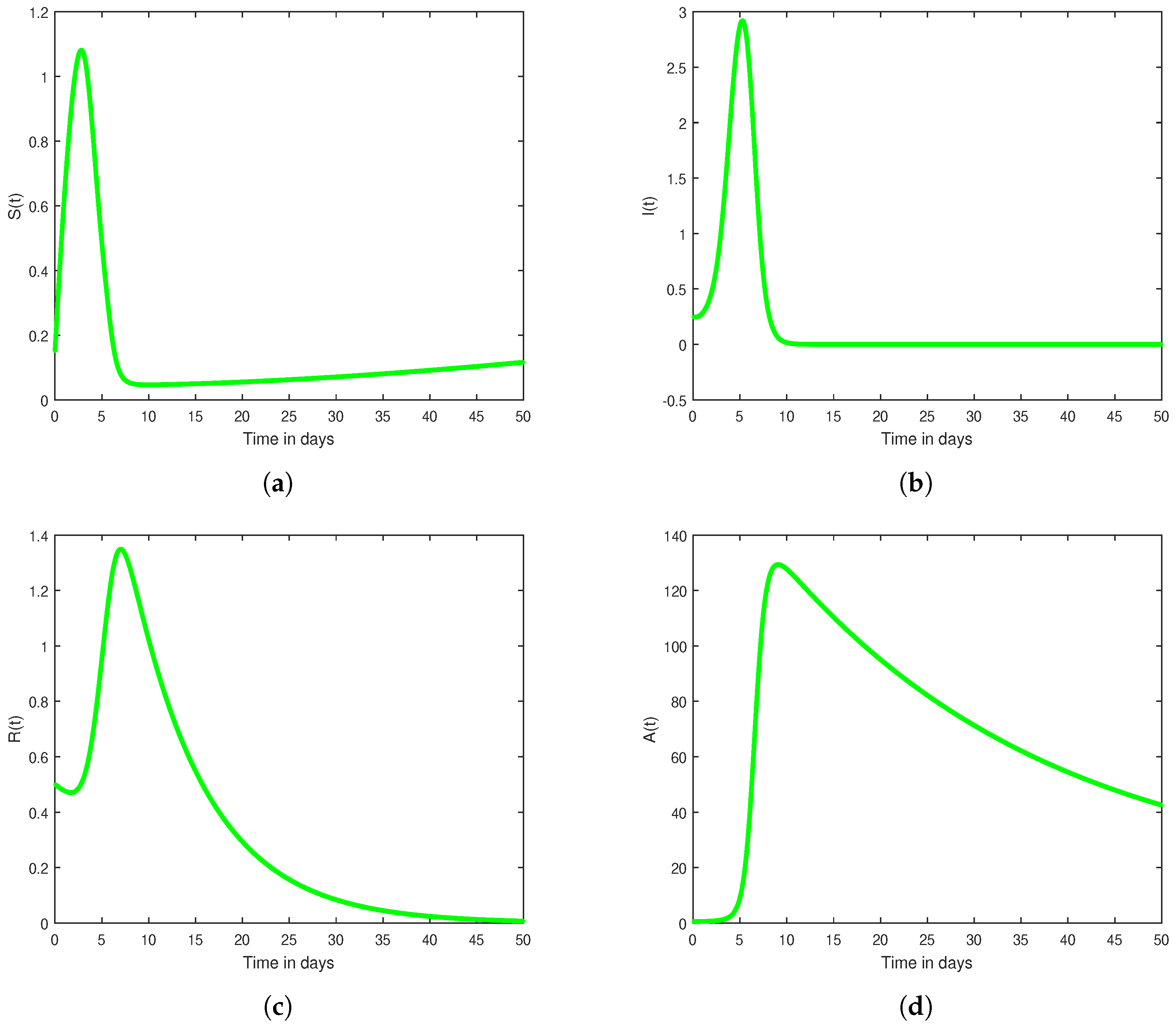
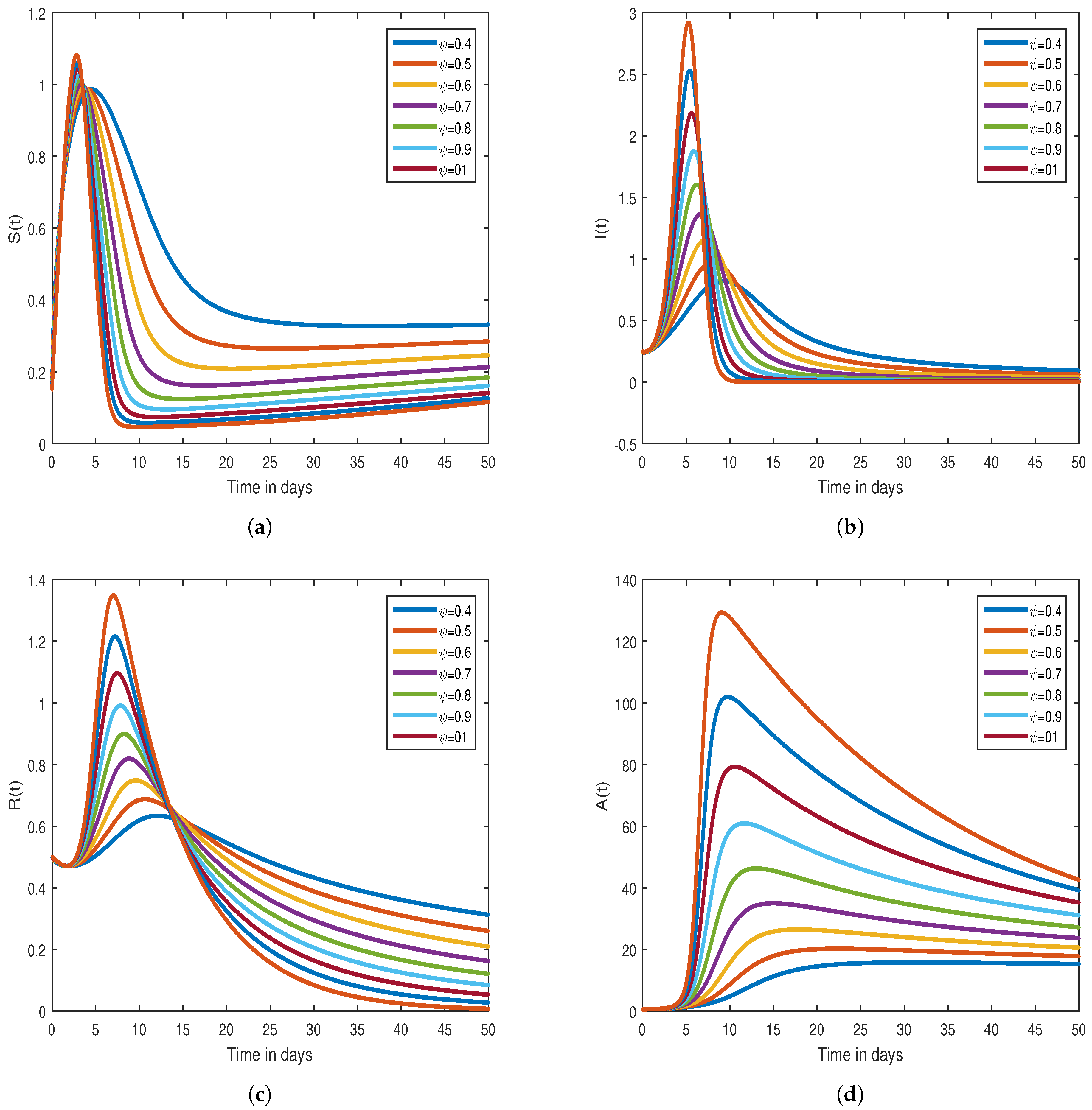
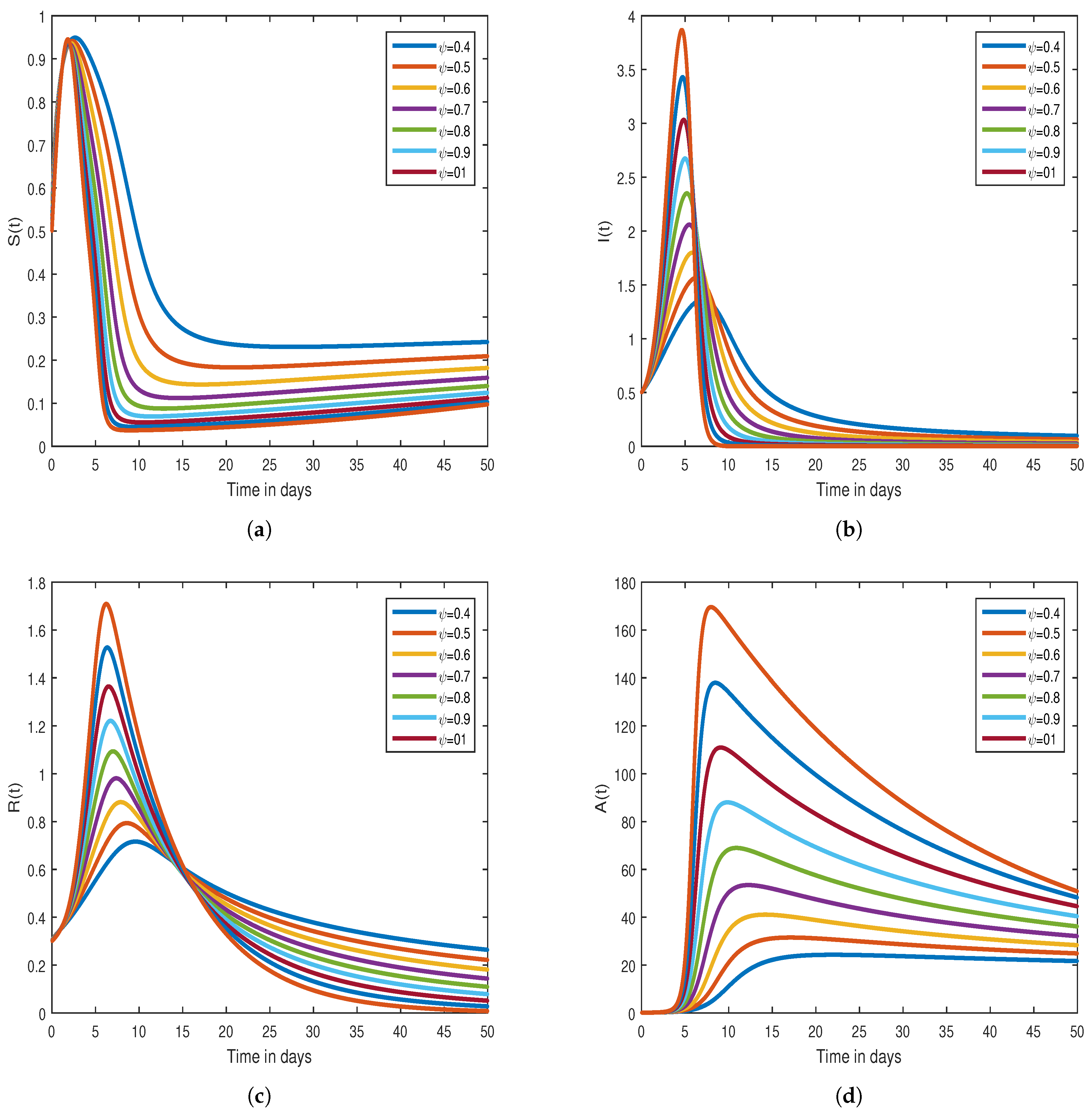
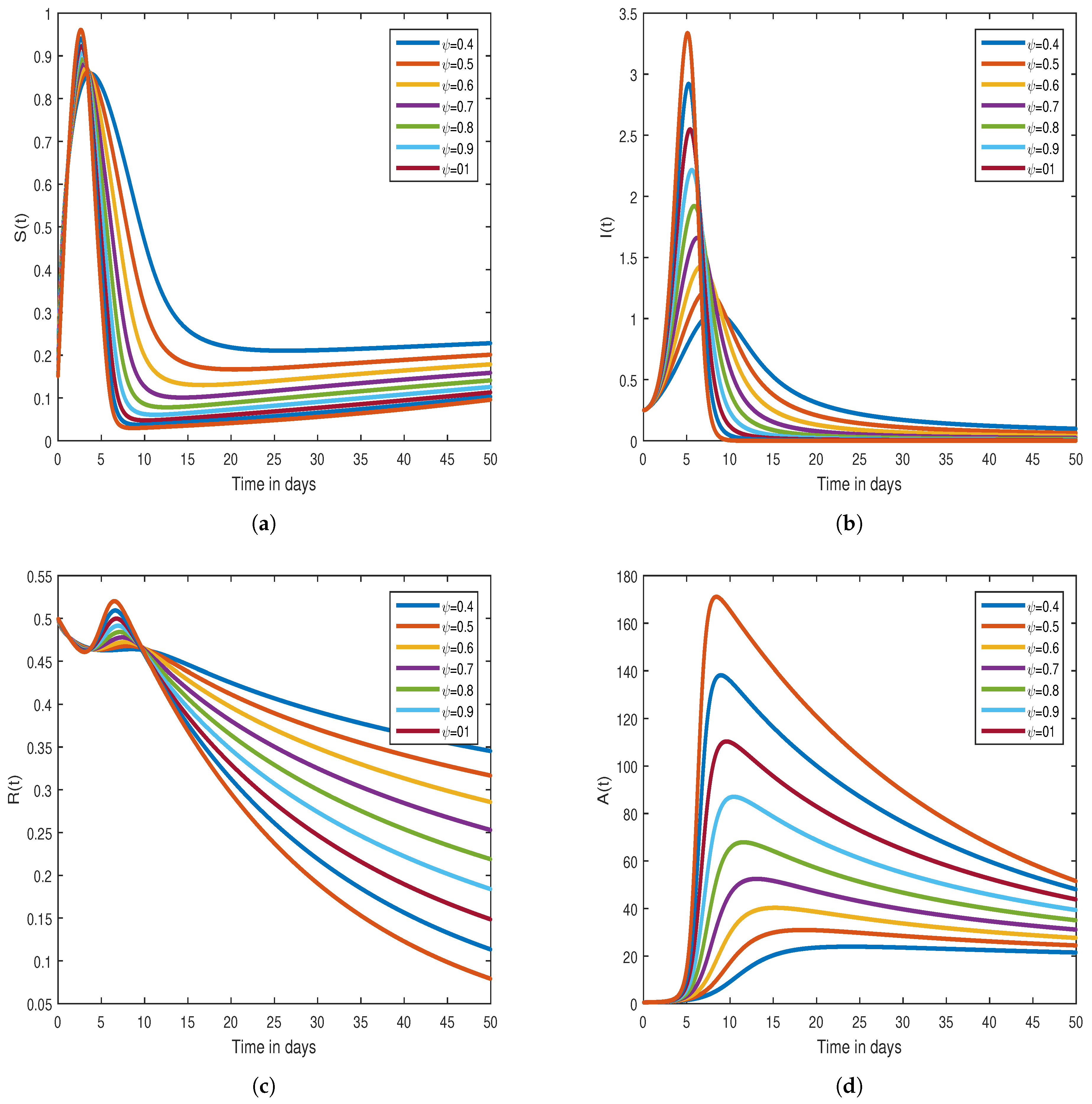
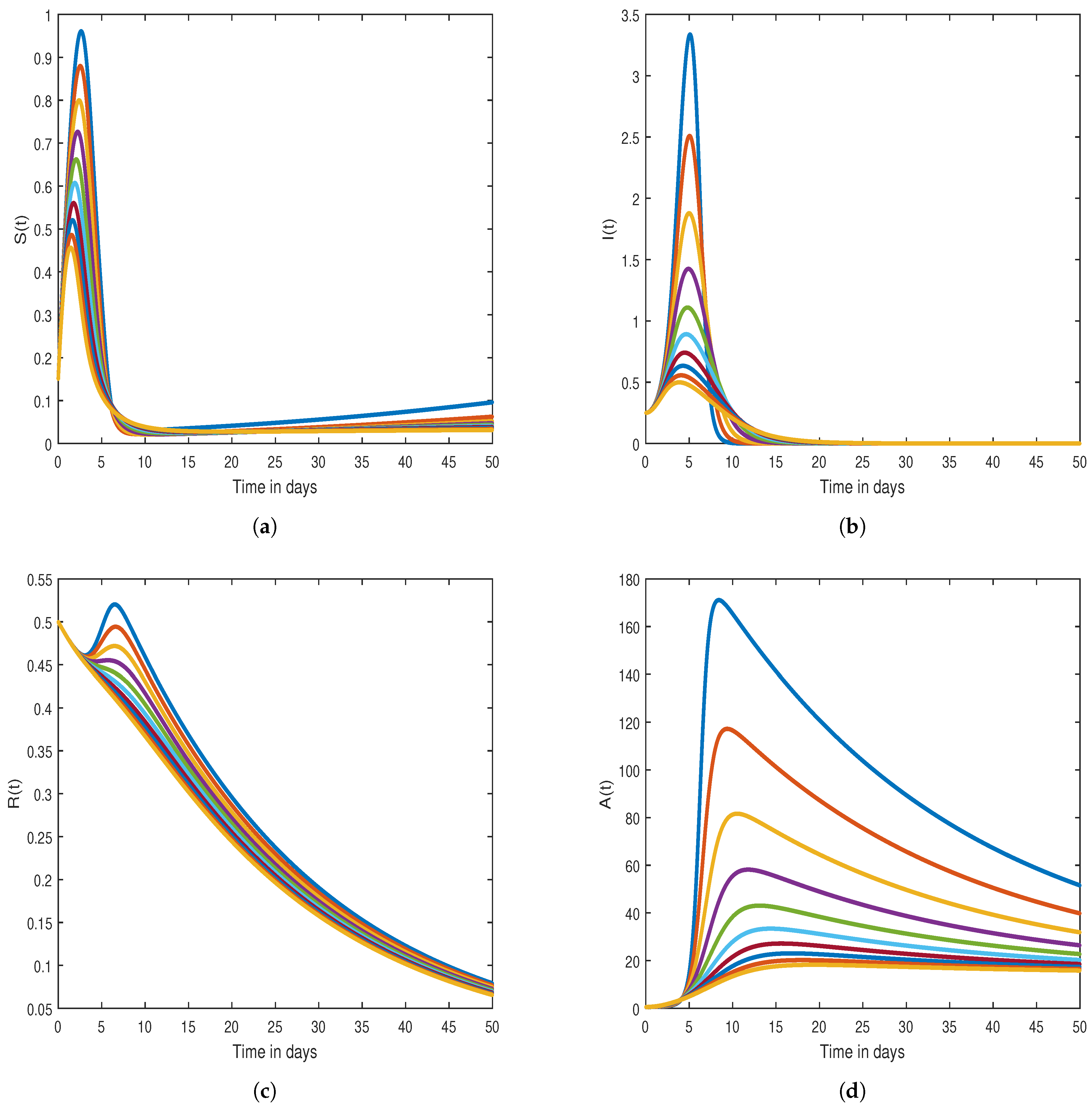
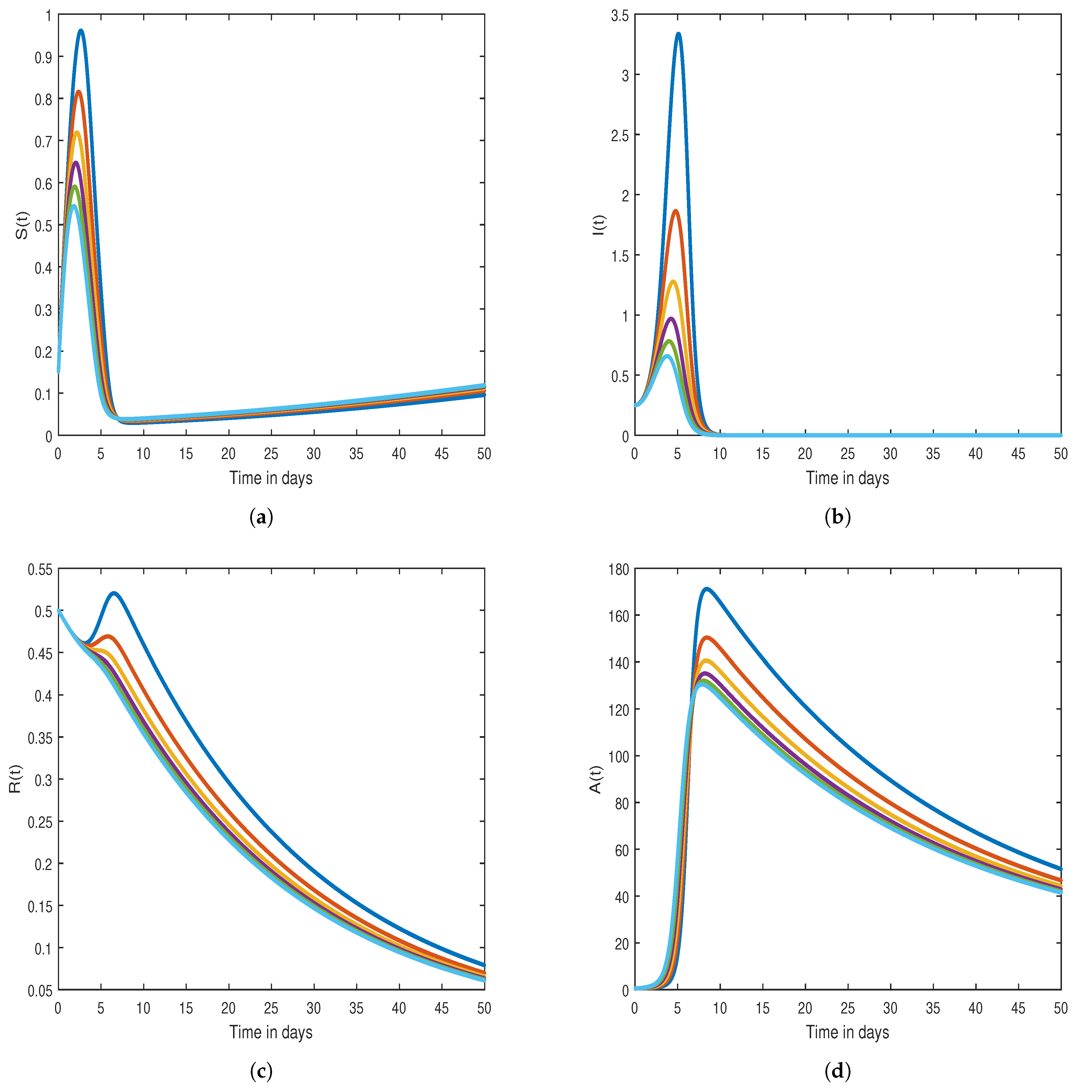
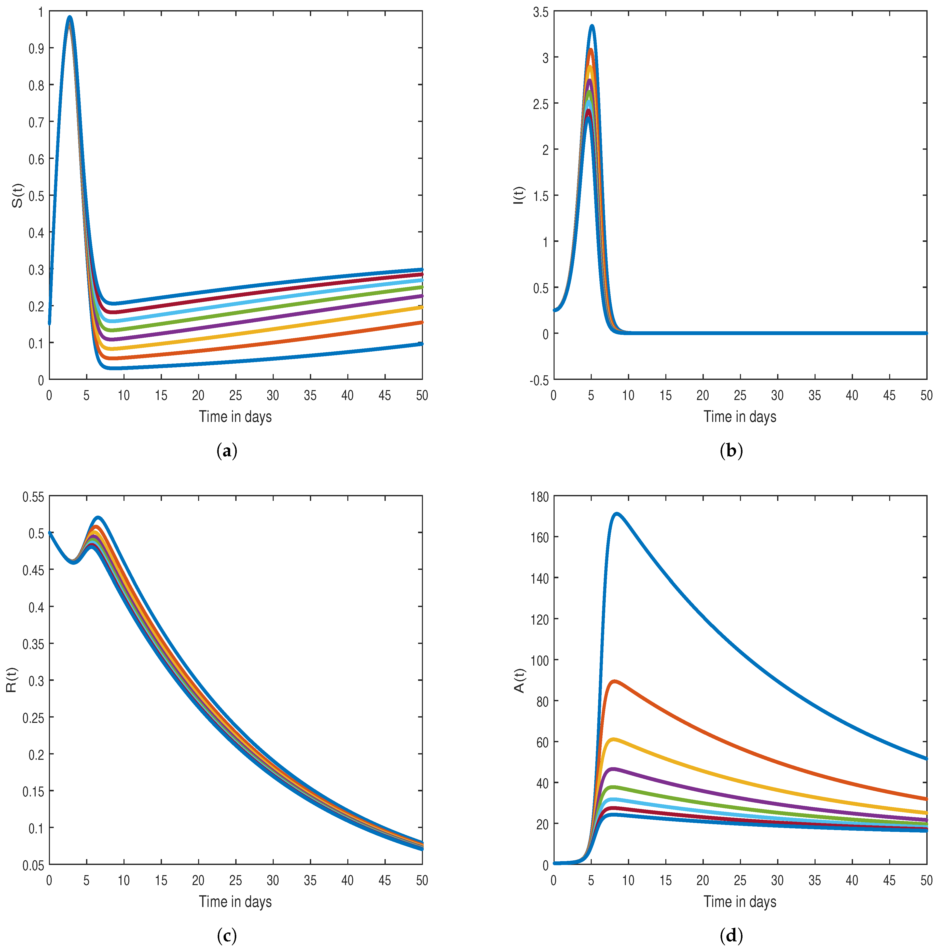
7. Graphical Results

A numerical simulation of the Caputo fractional antidotal computer virus model (1) is presented in this section, which is carried out with the values S ( 0 ) = 0.15 , I ( 0 ) = 0.25 , R ( 0 ) = 0.5 , and A ( 0 ) = 0.5 as the starting values. In this model, the parameters’ values are chosen to be Π = 0.5 , α = 0.1 , β = 0.5 , μ = 0.035 , c = 0.09 , γ = 0.01 , and δ = 0.015 . A Matlab-based generalized Haar wavelet numerical scheme is used for the numerical simulation. Profiles for the classical version of the deterministic model for the behavior of each state variable are shown in Figure 1. To observe the behavior of the considered population groups according to their disease status, the results are first plotted based on different values of ψ , as shown in Figure 2, Figure 3 and Figure 4.
It can be seen that there is an exponential decrease in the susceptible and infected population after the maximum is reached, as depicted in the aforementioned figures. The longer incubation period of fully developed symptoms is responsible for this effect from a biological standpoint. Compared with infected and susceptible populations, the recovered population increases around t = 15 days and then decreases over time. Moreover, the population of noninfected computers with effective antivirus programs increases rapidly and then declines slowly to reach equilibrium. Finally, the effect of the different parameters on each of the state variables is shown in Figure 5, Figure 6, Figure 7 and Figure 8.

8. Concluding Remarks

Mathematical models play a crucial role in computer network security by providing early warnings of viruses. Accordingly, kill signals allow users to take measures against viruses. We aim to understand how fractional derivatives can benefit memory and how they can help with computer virus problems. The generalized mean value theorem can be used to prove the existence, uniqueness, and boundedness of the solutions for the fractional-order SIRA model on the basis of [42]. For the purpose of demonstrating the effectiveness of the fractional-order ψ , simulation results were generated with Matlab software. As far as computer security and users are concerned, we believe that our results are very helpful in preventing virus spread. Nonlinear equations can be approximated iteratively using Haar wavelet collocation. Nonlinear problems can be solved efficiently and effectively using Haar wavelet collocation methods. It could become a powerful tool for solving nonlinear problems in science and engineering if Haar wavelet collocation methods are combined with high-performance computing software such as Mathematica, MATLAB, etc. The extension of the model is possible by considering the Hilfer fractional operator and comparing the results with the Caputo operator. Moreover, we can reformulate the model by incorporating the noise terms, and the model in this case will become a stochastic model. Keeping in view the sensitivity analysis of our model, one can apply optimal control theory as well.

Author Contributions

Methodology, R.Z.; Software, A.K.; Validation, U.W.H.; Investigation, H.K.; Writing—original draft, I.A.; Project administration, U.W.H. All authors have read and agreed to the published version of the manuscript.

Funding

This research received no external funding.

Data Availability Statement

Not applicable.

Acknowledgments

This research project was supported by the Thailand Science Research and Innovation (TSRI). Basic Research Fund: Fiscal year 2022 under project number FRB650048/0164. The first author appreciates the support provided by Petchra Pra Jom Klao Research Scholarship, by King Mongkut’s University of Technology Thonburi, Thailand. The authors also acknowledge the support provided by KMUTT Research Laboratory of Atmospheric, Oceanic Prediction and Infectious Disease Modeling (K@TOP IDM).

Conflicts of Interest

The authors declare no conflict of interest.

References

  1. Han, X.; Tan, Q. Dynamical behavior of computer virus on Internet. Appl. Math. Comput. 2010, 217, 2520–2526. [Google Scholar] [CrossRef]
  2. Kim, J.; Radhakrishana, S.; Jang, J. Cost optimization in SIS model of worm infection. ETRI J. 2006, 28, 692–695. [Google Scholar] [CrossRef]
  3. Piqueira, J.R.C.; Araujo, V.O. A modified epidemiological model for computer viruses. Appl. Math. Comput. 2009, 213, 355–360. [Google Scholar] [CrossRef]
  4. Billings, L.; Spears, W.M.; Schwartz, I.B. A unified prediction of computer virus spread in connected networks. Phys. Lett. A 2002, 297, 261–266. [Google Scholar] [CrossRef]
  5. Gan, C.; Yang, X.; Zhu, Q.; Jin, J.; He, L. The spread of computer virus under the effect of external computers. Nonlinear Dyn. 2013, 73, 1615–1620. [Google Scholar] [CrossRef]
  6. Gan, C.; Yang, X.; Liu, W.; Zhu, Q. A propagation model of computer virus with nonlinear vaccination probability. Commun. Nonlinear Sci. Numer. Simul. 2014, 19, 92–100. [Google Scholar] [CrossRef]
  7. Muroya, Y.; Enatsu, Y.; Li, H. Global stability of a delayed SIRS computer virus propagation model. Int. J. Comput. Math. 2013, 91, 347–367. [Google Scholar] [CrossRef]
  8. Mishra, B.K.; Pandey, S.K. Dynamic model of worms with vertical transmission in computer network. Appl. Math. Comput. 2011, 217, 8438–8446. [Google Scholar] [CrossRef]
  9. Yang, L.X.; Yang, X.; Wen, L.; Liu, J. A novel computer virus propagation model and its dynamics. Int. J. Comput. Math. 2012, 89, 2307–2314. [Google Scholar] [CrossRef]
  10. Yang, L.X.; Yang, X. The spread of computer viruses under the influence of removable storage devices. Appl. Math. Comput. 2012, 219, 3914–3922. [Google Scholar] [CrossRef]
  11. Feng, L.; Liao, X.; Li, H.; Han, Q. Hopf bifurcation analysis of a delayed viral infection model in computer networks. Math. Comput. Model. 2012, 56, 167–179. [Google Scholar] [CrossRef]
  12. Ren, J.; Yang, X.; Yang, L.-X.; Xu, Y.; Yang, F. A delayed computer virus propagation model and its dynamics. Chaos Solitons Fractals 2012, 45, 74–79. [Google Scholar] [CrossRef]
  13. Mishra, B.K.; Jha, N. Fix period of temporary immunity after run of anti-malicious software on computer nodes. Appl. Math. Comput. 2007, 190, 1207–1212. [Google Scholar]
  14. Yang, L.X.; Draief, M.; Yang, X.F. The optimal dynamics immunization under a controlled heterogeneous node-based SIRS model. Physica A 2016, 450, 403–415. [Google Scholar] [CrossRef]
  15. Zarin, R.; Khaliq, H.; Khan, A.; Khan, D.; Akgül, A.; Humphries, U.W. Deterministic and fractional modeling of a computer virus propagation. Results Phys. 2022, 33, 105130. [Google Scholar] [CrossRef]
  16. Zhu, Q.Y.; Yang, X.F.; Yang, L.X. A mixing propagation model of computer viruses and countermeasures. Nonlinear Dyn. 2013, 73, 1433–1441. [Google Scholar] [CrossRef]
  17. Kephart, J.O.; White, S.R. Measure and Modeling Computer Virus Prevalence. In Proceedings of the IEEE Computer Society Symposium Research in Security and Privacy, Oakland, CA, USA, 24–26 May 1993. [Google Scholar]
  18. Podlubny, I. Fractional Differential Equations; Academic Press Elsevier: New York, NY, USA, 1999. [Google Scholar]
  19. Pinto, C.M.A.; Machado, J.A.T. Fractional dynamics of computer virus propagation. Math. Probl. Eng. 2014, 2014, 476502. [Google Scholar] [CrossRef] [Green Version]
  20. Ansari, M.A.; Arora, D.; Ansari, S.P. Chaos control and synchronization of fractional order delay-varying computer virus propagation model. Math. Meth. Appl. Sci. 2016, 39, 1197–1205. [Google Scholar] [CrossRef]
  21. Fernandez, A.; Baleanu, D.; Srivastava, H.M. Series representations for fractional-calculus operators involving generalised Mittag-Leffler functions. Commun. Nonlinear Sci. Numer. Simul. 2019, 67, 517–527. [Google Scholar] [CrossRef] [Green Version]
  22. Khan, A.; Zarin, R.; Khan, S.; Saeed, A.; Gul, T.; Humphries, U.W. Fractional dynamics and stability analysis of COVID-19 pandemic model under the harmonic mean type incidence rate. Comput. Methods Biomech. Biomed. Eng. 2022, 25, 619–640. [Google Scholar] [CrossRef]
  23. Almeida, R.; Morgado, M.L. Analysis and numerical approximation of tempered fractional calculus of variations problems. J. Comput. Appl. Math. 2019, 361, 1–12. [Google Scholar] [CrossRef]
  24. Fernandez, A.; Ozarslan, M.A.; Baleanu, D. On fractional calculus with general analytic kernels. Appl. Math. Comput. 2019, 354, 248–265. [Google Scholar] [CrossRef] [Green Version]
  25. Jitsinchayakul, S.; Zarin, R.; Khan, A.; Yusuf, A.; Zaman, G.; Sulaiman, T.A. Fractional modeling of COVID-19 epidemic model with harmonic mean type incidence rate. Open Phys. 2021, 19, 693–709. [Google Scholar] [CrossRef]
  26. Zarin, R.; Ahmed, I.; Kumam, P.; Zeb, A.; Din, A. Fractional modeling and optimal control analysis of rabies virus under the convex incidence rate. Results Phys. 2021, 28, 104665. [Google Scholar] [CrossRef]
  27. Zarin, R. Modeling and numerical analysis of fractional order hepatitis B virus model with harmonic mean type incidence rate. Comput. Methods Biomech. Biomed. Eng. 2022, 1–16. [Google Scholar] [CrossRef] [PubMed]
  28. Kumar, D.; Agarwal, R.P.; Singh, J. A modified numerical scheme and convergence analysis for fractional model of Lienard’s equation. J. Comput. Appl. Math. 2018, 339, 405–413. [Google Scholar] [CrossRef]
  29. Zarin, R.; Khan, A.; Inc, M.; Humphries, U.W.; Karite, T. Dynamics of five grade leishmania epidemic model using fractional operator with Mittag–Leffler kernel. Chaos Solitons Fractals 2021, 147, 110985. [Google Scholar] [CrossRef]
  30. Matar, M.M.; Abbas, M.I.; Alzabut, J.; Kaabar, M.K.A.; Etemad, S.; Rezapour, S. Investigation of the p-Laplacian nonperiodic nonlinear boundary value problem via generalized Caputo fractional derivatives. Adv. Differ. Equ. 2021, 2021, 68. [Google Scholar] [CrossRef]
  31. Ahmad, M.; Jiang, J.; Zada, A.; Shah, S.O.; Xu, J. Analysis of implicit coupled system of fractional differential equations involving Katugampola–Caputo fractional derivative. Complexity 2020, 2020, 9285686. [Google Scholar] [CrossRef] [Green Version]
  32. Gu, Y.; Khan, M.; Zarin, R.; Khan, A.; Yusuf, A.; Humphries, U.W. Mathematical analysis of a new nonlinear dengue epidemic model via deterministic and fractional approach. Alex. Eng. J. 2023, 67, 1–21. [Google Scholar] [CrossRef]
  33. Liu, P.; Din, A.; Zarin, R. Numerical dynamics and fractional modeling of hepatitis B virus model with non-singular and non-local kernels. Results Phys. 2022, 39, 105757. [Google Scholar] [CrossRef]
  34. Caputo, M.; Mainardi, F. A new dissipation model based on memory mechanism. Pure Appl. Geophys. 1971, 91, 134–147. [Google Scholar] [CrossRef]
  35. Caputo, M.; Fabricio, M. A new definition of fractional derivative without singular kernel. Prog. Fract. Differ. Appl. 2015, 1, 73–85. [Google Scholar]
  36. Shi, Z.; Deng, L.Y.; Chen, Q.J. Numerical solution of differential equations by using Haar wavelets. In Proceedings of the 2007 International Conference on Wavelet Analysis and Pattern Recognition, Beijing, China, 2–4 November 2007; 2007; Volume 3, pp. 1039–1044. [Google Scholar]
  37. Shah, K.; Khan, Z.A.; Ali, A.; Amin, R.; Khan, H.; Khan, A. Haar wavelet collocation approach for the solution of fractional order COVID-19 model using Caputo derivative. Alex. Eng. J. 2020, 59, 3221–3231. [Google Scholar] [CrossRef]
  38. Prakash, B.; Setia, A.; Alapatt, D. Numerical solution of nonlinear fractional SEIR epidemic model by using Haar wavelets. J. Comput. Sci. 2017, 22, 109–118. [Google Scholar] [CrossRef]
  39. Makhlouf, A.B.; Mchiri, L. Some results on the study of Caputo-Hadamard fractional stochastic differential equations. Chaos Solitons Fractals 2022, 155, 111757. [Google Scholar] [CrossRef]
  40. Caraballo, T.; Mchiri, L.; Rhaima, M. Ulam-Hyers-Rassias stability of neutral stochastic functional differential equations. Stochastics 2022, 94, 959–971. [Google Scholar] [CrossRef]
  41. Makhlouf, A.B.; Mchiri, L.; Arfaoui, H.; Dhahri, S.; El-Hady, E.S.; Cherif, B. Hadamard Itˆo-Doob stochastic fractional order systems. Discret. Contin. Dyn. Syst.-S 2022. [Google Scholar] [CrossRef]
  42. Khanh, N.H. Dynamical analysis and approximate iterative solutions of an antidotal computer virus model. Int. J. Appl. Comput. Math. 2017, 3, 829–841. [Google Scholar] [CrossRef]
  43. Lepik, Ü. Numerical solution of differential equations using Haar wavelets. Math. Comput. Simul. 2005, 68, 127–143. [Google Scholar] [CrossRef]
  44. Shiralashetti, S.C.; Mundewadi, R.A.; Naregal, S.S.; Veeresh, B. Haar Wavelet Collocation Method for the Numerical Solution of Nonlinear Volterra-Fredholm-Hammerstein Integral Equations. Glob. J. Pure Appl. Math. 2017, 13, 463–474. [Google Scholar]
  45. Majak, J.; Shvartsman, B.S.; Kirs, M.; Pohlak, M.; Herranen, H. Convergence theorem for the Haar wavelet based discretization method. Compos. Struct. 2015, 126, 227–232. [Google Scholar] [CrossRef]
Figure 1. Profiles for the classical version of the deterministic model for behavior of each state variable. (a) The susceptible computer. (b) The removed or recovered computer. (c) The removed or recovered computer. (d) The noninfected computers equipped with effective antivirus programs.
Symmetry 15 00621 g001
Figure 2. Profiles for the Caputo version of the fractional model at ψ = 0.4 , ψ = 0.5 , ψ = 0.6 , ψ = 0.7 , ψ = 0.8 , ψ = 0.9 , and ψ = 01 for the behavior of each state variable. In this case, the numerical values of the parameters and variables are Π = 0.5 ; α = 0.1 ; β = 0.5 ; λ = 0.07 ; μ = 0.035 ; c = 0.09 ; ϵ = 0.009 ; γ = 0.01 ; and δ = 0.015 ; additionally, S = 0.15 , I = 0.25 , R = 0.5 , and A = 0.5 . (a) The susceptible computer. (b) The removed or recovered computer. (c) The removed or recovered computer. (d) The noninfected computers equipped with effective antivirus programs.
Symmetry 15 00621 g002
Figure 3. Profiles for the Caputo version of the fractional model at ψ = 0.4 , ψ = 0.5 , ψ = 0.6 , ψ = 0.7 , ψ = 0.8 , ψ = 0.9 , and ψ = 01 for the behavior of each state variable. In this case, the numerical values of the parameters and variables are Π = 0.5 ; α = 0.1 ; β = 0.5 ; λ = 0.07 ; μ = 0.035 ; c = 0.09 ; ϵ = 0.009 ; γ = 0.01 ; and δ = 0.015 ; additionally, S = 0.15 , I = 0.25 , R = 0.5 , and A = 0.5 . (a) The susceptible computer. (b) The removed or recovered computer. (c) The removed or recovered computer. (d) The noninfected computers equipped with effective antivirus programs.
Symmetry 15 00621 g003
Figure 4. Profiles for the Caputo version of the fractional model at ψ = 0.4 , ψ = 0.5 , ψ = 0.6 , ψ = 0.7 , ψ = 0.8 , ψ = 0.9 , and ψ = 01 for the behavior of each state variable. In this case, the numerical values of the parameters and variables are Π = 0.5 ; α = 0.1 ; β = 0.5 ; λ = 0.07 ; μ = 0.035 ; c = 0.09 ; ϵ = 0.009 ; γ = 0.01 ; and δ = 0.015 ; additionally, S = 0.15 , I = 0.25 , R = 0.5 , and A = 0.5 . (a) The susceptible computer. (b) The removed or recovered computer. (c) The removed or recovered computer. (d) The noninfected computers equipped with effective antivirus programs.
Symmetry 15 00621 g004
Figure 5. Impact of the parameter δ on each state variable for fractional-order ψ = 1 and δ = 0.015 : 0.15 : 1.0 . (a) The susceptible computer. (b) The removed or recovered computer. (c) The removed or recovered computer. (d) The noninfected computers equipped with effective antivirus programs.
Symmetry 15 00621 g005
Figure 6. Impact of the parameter α on each state variable for fractional-order ψ = 1 and α = 0.1 : 0.1 : 1.0 . (a) The susceptible computer. (b) The removed or recovered computer. (c) The removed or recovered computer. (d) The noninfected computers equipped with effective antivirus programs.
Symmetry 15 00621 g006
Figure 7. Impact of the parameter β on each state variable for fractional-order ψ = 1 and β = 0.5 : 0.3 : 2.0 . (a) The susceptible computer. (b) The removed or recovered computer. (c) The removed or recovered computer. (d) The noninfected computers equipped with effective antivirus programs.
Symmetry 15 00621 g007
Figure 8. Impact of the parameter γ on each state variable for fractional-order ψ = 1 and γ = 0.01 : 0.01 : 0.08 . (a) The susceptible computer. (b) The removed or recovered computer. (c) The removed or recovered computer. (d) The noninfected computers equipped with effective antivirus programs.
Symmetry 15 00621 g008
Disclaimer/Publisher’s Note: The statements, opinions and data contained in all publications are solely those of the individual author(s) and contributor(s) and not of MDPI and/or the editor(s). MDPI and/or the editor(s) disclaim responsibility for any injury to people or property resulting from any ideas, methods, instructions or products referred to in the content.

