Article

Prioritization of Thermal Energy Storage Techniques Using TOPSIS Method Based on Correlation Coefficient for Interval-Valued Intuitionistic Fuzzy Hypersoft Set

by
Rana Muhammad Zulqarnain
1,
Wen-Xiu Ma
1,2,3,4,*,
Imran Siddique
5,
Alhanouf Alburaikan
6,
Hamiden Abd El-Wahed Khalifa
6,7 and
Agaeb Mahal Alanzi
6,*
1
School of Mathematical Sciences, Zhejiang Normal University, Jinhua 321004, China
2
Department of Mathematics, King Abdulaziz University, Jeddah 21589, Saudi Arabia
3
Department of Mathematics and Statistics, University of South Florida, Tampa, FL 33620-5700, USA
4
School of Mathematical and Statistical Sciences, North-West University, Mafikeng Campus, Private Bag X2046, Mmabatho 2735, South Africa
5
Department of Mathematics, University of Management and Technology, Lahore 54770, Pakistan
6
Department of Mathematics, College of Science and Arts, Qassim University, Al-Badaya 51951, Saudi Arabia
7
Department of Operations and Management Research, Faculty of Graduate Studies for Statistical Research, Cairo University, Giza 12613, Egypt
*
Authors to whom correspondence should be addressed.
Symmetry 2023, 15(3), 615; https://doi.org/10.3390/sym15030615
Submission received: 4 February 2023 / Revised: 21 February 2023 / Accepted: 25 February 2023 / Published: 28 February 2023
(This article belongs to the Special Issue Recent Advances in Fuzzy Optimization Methods and Models)

Abstract

:
The correlation between two disparate variables conquers a significant habitation in statistics. The concept of correlation coefficient (CC) is one of the well-known indicators, but it is not used in interval-valued intuitionistic fuzzy hypersoft set (IVIFHSS) information. It is a generalization of interval-valued intuitionistic fuzzy soft sets and a refined extension of intuitionistic fuzzy hypersoft sets. However, using the CC and weighted correlation coefficient (WCC) has not yet been explored for IVIFHSS information. The core objective of this research is to present the correlation coefficient (CC) and weighted correlation coefficient (WCC) for interval-valued intuitionistic fuzzy hypersoft sets (IVIFHSS) and their mandatory properties. A prioritization technique for order preference by similarity to the ideal solution (TOPSIS) is developed based on proposed correlation measures. To ensure the symmetry of the developed scheme, we consider mathematical clarifications of correlation contractions. Based on assessments, it conceded vibrant multi-attribute decision-making (MADM) methodology with the most substantial significance. In addition, a statistical illustration is designated to regulate the operative usage of a decision-making configuration in thermal energy storage techniques. The productivity of the advocated algorithm is more reliable than existing replicas to control the favorable configurations of the premeditated study.

1. Introduction

The proficiency to store energy and consumption in the future is one of the recipes for repossessing massive amounts of renewable energy on the grid. There are copious types of systems to store energy, including mechanical, electrical, chemical, electrochemical, and thermal. Thermal energy storage (TES) is a method for compliance with thermal energy by warming or preserving the storage abstemiously so that the stored energy can be used for subsequent central heating and preservation solicitations and power generation. Energy storage structures are used primarily in construction and engineering practices. In these presentations, almost half the energy is heating, and its mandate can fluctuate daily. Thus, TES structures can support stability mandates and daily, weekly, and periodic energy capitals. They can also moderate eventual affirmation, energy ingestion, carbon dioxide releases, and expenditures while clarifying the whole efficiency of energy structures. Moreover, the renovation and storage of pliable renewable energy cradles in preparing thermal energy support increase the portion of renewable energy in the energy mingling. TES conversion is mainly significant for power storing, combined with concentrated solar plants, which can stock solar heat to produce electricity without sunlight. TES is essential in several industrial presentations. One of the real-world problems convoluted in solar energy schemes is the necessity for operational capital by which it can be stockpiled. Comparable difficulties ascend in excess heat recovery schemes everywhere, and surplus heat accessibility and exploitation phases fluctuate. Heat storing can also be pragmatic to maximum kinds of constructions where the heating system mandate is extraordinary and electrical energy notices permit heat storing to contest with other arrangements of the heating system. Numerous kinds of transaction structures exist, and several novel improvements are captivating in this expertise. Energy storage technology supports storing energy to elucidate future energy complications. The thermal energy storage technique (TEST) is the most imperative energy technology. Dincer [1] demonstrated in his study that TEST is an essential energy storage skill for energy conversion. Pecuniary intentions have a stimulus on energy transformation schemes, which makes the TEST even more prominent. Kocak et al. [2] discovered that the TEST is a beneficial procedure with several uses in engineering. This TES solution can potentially escalate thermal energy apparatus usage on an elective foundation. There are commonly four different forms of TEST: sensible TEST, latent TEST, thermochemical TEST, and underground TEST. The prerequisite storage period typically determines the variety of the TEST.
The correlation coefficient plays an important role in statistics and industrial engineering. With correlation exploration, the mutual association of two variables can be used to judge the interdependence of the two variables. While probabilistic approaches are applied to numerous real-world industrial complications, probabilistic schemes have some hurdles. The prospect of a procedure is contingent on the massive quantity of information composed, which is arbitrary. However, generally, composite structures have a lot of imprecise hesitations, making it tough to attain exact possibility dealings. Thus, due to restricted computable facts, consequences built on the probability model do not constantly deliver convenient facts for specialists. In addition, occasionally, statistics are insufficient to correct procedure information in everyday use. Due to the above limitations, outcomes founded on the possibility system are not continuously offered to professionals. Thus, probabilistic techniques are habitually not abundant to report this intrinsic vagueness in the statistics. Because of all the concrete expectations, criteria, or arrangements that originate with it, MADM has been termed as the most effective and efficient mode to accomplish appropriate alternatives. A comprehensive estimation happens when representative intents and restrictions are often uncertain or imperfect. Zadeh [3] proposed the concept of fuzzy sets (FS) to prove this false and contradictory data. It is authoritative to condense redundant and apprehensive DM difficulties. The FS model has been usually used in different fields. Cavallaro [4] introduced the fuzzy TOPSIS to judge TES in intensive solar enlargements. Turksen [5] presented the concept of interval-valued fuzzy sets (IVFS) as a leeway of FS, where the membership value is represented in interval form rather than numbers. The IVFS describes the uncertainty more abundantly than FS. Therefore, it is substantial to use an IVFS in fuzzy control. Yu [6] established fuzzy numbers’ correlation coefficient (CC) to extend the connection among fuzzy numbers. Pekaslan et al. [7] proposed an online learning method that updates the input fuzzy sets of an NSFLS using a sequence of observations, enabling the system to handle variations in input-related noise commonly found in real-world applications. Ashtiani et al. [8] extended the TOPSIS method in the IVFS environment and used it to resolve MCDM hurdles.
Traditional FS and IVFS cannot contest the stable sophistication of DM assessment specialists on membership degrees (MD) and non-membership degrees (NMD). Atanassov [9] presented the theory of intuitionistic fuzzy sets (IFS), a generality of FS theory. Rouyendegh et al. [10] introduced the TOPSIS method for IFS and utilized it in green supply chain management. Atanassov [11] extended his developed IFS theory to interval-valued IFS (IVIFS) with significant properties. Tang et al. [12] developed a novel algorithm for IFS based on residual intuitionistic implications known as intuitionistic fuzzy entropy derived symmetric implicational and presented its desirable properties. Hung and Wu [13] planned a centroid system to compute the CC of IFS and protracted this technique to IVIFS. Bustince and Burillo [14] demonstrated the CC for IVIFS and presented the decomposition proposals of CC. Hong [15] and Mitchell [16] proposed the decomposition theorems on CC for IFS and IVIFS. Zhang and Yu [17] developed the TOPSIS technique for IVIFS to resolve MADM concerns. Jana et al. [18] introduced the hybrid Dombi AOs for IFS and developed a MADM technique based on their presented AOs. Paul et al. [19] introduced the VIKOR and DEMATEL approaches for Pythagorean fuzzy sets and utilized their developed methodologies in sustainable carbon-dioxide storage assessment in geological media. Jana et al. [20] developed the Dombi operations for q-rung orthopair fuzzy numbers and introduced several AOs with the MADM technique. Singh et al. [21] settled another two-parameter generality of CC on IFS and applied the planned method to multi-attribute group decision-making (MAGDM) problems. The Atanassov model contracts only with scarce facts due to MD and NMD; however, IFS sometimes cannot handle contradictory and misinformation. These models have extensive applications, but none of the above structures can handle the parametric values of the alternative. Molodtsov [22] planned a general mathematical tool entitled soft sets (SS) to contract with ambiguous, abstruse, equivocal matters. Maji et al. [23] bonded two persistent models, FS and SS, and the projected fuzzy soft set (FSS) theory. They also extended the FSS theory to intuitionistic FSS (IFSS) [24] with important operations and their properties. Garg and Arora [25] developed the correlation-based TOPSIS methodology for IFSS. Jiang et al. [26] prolonged the interval-valued IFSS (IVIFSS) with basic operations and discussed their properties. Ma et al. [27] developed a novel DM technique using choice and score values for IVIFSS. Khan et al. [28] introduced basic operations for generalized IVIFSS and developed a MADM plan to resolve real-life complexities. Zulqarnain et al. [29] extended the TOPSIS method and aggregation operators (AOs) to resolve MADM complications under the considered scenario. Garg and Arora [30] presented nonlinear programming based on TOPSIS to resolve MADM problems. Zulqarnain et al. [31,32,33] developed the innovative DM methodology for interval-valued fuzzy soft matrix (IVFSM) and utilized it in decision-making. They also presented the comparison between fuzzy soft matrices and IVFSM. Dayan and Zulqarnain [34] proposed the generalized IVFSM with basic operations and their properties.
Models with SS settings are compact, with single-parameter assessments, while hypersoft sets (HSS), leeway for SS, and contraction have multiparameter approximations. The SS cannot state where the parameters should be divided into more subspecialties. In many DM states, the simulated parameters should be defined as sub-parameters. Smarandache [35] protracted the SS to an HSS, the most corporate model for dealing with several sub-features of well-thought-out parameters. Rahman et al. [36] developed SM for the possibility IFHSS. They also introduced some operations for fuzzy HSS with their properties [37] to resolve MADM complications. Zulqarnain et al. [38,39] developed the aggregation operators for IFHSS and discussed their properties. They also extended the TOPSIS method based on CC under their considered environment to resolve MADM hurdles. Debnath [40] combined the HSS with IVIFS, presented the idea of IVIFHSS, and discussed the favorable operations with their elementary properties. Zulqarnain et al. [41] extended the concept of IVIFHSS, introduced the AOs for IVIFHSS, and established a novel DM method for material selection. Zulqarnain et al. [42] introduced the MCGDM approach for interaction aggregation operators for IVIFHSS. An enhanced incorporated association would entice spies to debate these flaws with sketchy, unimaginable, and asymmetrical details. They demonstrate the significance of consideration, and IVIFHSS looks at the active part of DM by collecting a structure of affluence in a precise decision.

1.1. Motivation

The field of decision-making has undergone significant advancements in recent years, particularly in handling uncertainty and incomplete information. Interval-valued intuitionistic fuzzy hypersoft sets (IVIFHSS) have emerged as an important tool for addressing these challenges, combining the advantages of HSS and IVIFS, a fundamental scientific technique for managing reluctance, disparities, and incomplete data. The TOPSIS method is crucial in dealing with DM issues, as it transforms the specifications of public decisions for various objectives into a single analysis. It is worth noting that the CC has not been utilized in the literature on the hybridization of HSS and IVIFS. Therefore, the predominant TOPSIS technique neither measures composite interval-valued intuitionistic fuzzy hypersoft numbers (IVIFHSN) nor is it intentionally associated with MD and NMD. The influence of MD (NMD) on consequent TOPSIS techniques did not obstruct the whole development. In addition, the model categorizes the entire level of MD (NMD) functionality independent of the NMD(MD) functional level. Thus, the results are constrained by giving these correlation measures; therefore, the application bias of alternatives cannot be determined. To address such issues, we present CC and WCC for IVIFHSS, and we have developed the TOPSIS method to address MADM problems using the correlation measures developed. The predominant CC and WCC are transformed into exceptional circumstances of IVIFHSS. Therefore, it can be determined that the planned model is considerably more capable than the current TOPSIS techniques. Thus, the results of the prevalent model are unfavorable, and the favoritism of the alternative model cannot be adequately formulated. The TOPSIS method considered in [24] is insufficient to fact-check flexibly to get good ideas and solid results. Because it cannot calculate several sub-features of an alternative, on the other hand, the correlation-based TOPSIS approach in [34] can handle several subspecialties of alternatives. However, it can be processed as an intuitionistic fuzzy number rather than an interval-valued intuitionistic fuzzy number. The correlation-based TOPSIS method we have developed is one of the most versatile and capable techniques for MD and NMD to deal with uncertainty and misinformation by considering the sub-attributes in interval form.
The innovation of this study lies in developing a CC and WCC specifically designed for IVIFHSS. This addresses the limitation of the commonly used CC measure, which does not account for certain factors in DM protocols. The study also introduces a prioritization technique called TOPSIS, which uses the developed CC and WCC measures to rank order preferences based on similarity to the ideal solution. The study’s methodology is demonstrated through a statistical example, and comparative studies are presented to confirm the practicality and symmetry of the developed approach. The study’s contribution is developing a new strategy to DM in IVIFHSS, which is more reliable than existing models.

1.2. Contribution

The standard CC may not accurately reflect the competitive value of alternatives in DM protocols, as it does not account for certain factors. Therefore, to address this issue in the context of IVIFHSS, this study will introduce CC and WCC measures based on imprecise information. The study’s objectives are to:
Discuss the basic properties of informational energies for IVIFHSS settings. In fuzzy set theory, informational energies refer to the amount of information contained in a fuzzy set. In the context of IVIFHSS, the study aims to develop a framework for understanding the informational energies of this generalized form of fuzzy sets.
Develop new correlation measures, the CC and WCC, for IVIFHSNs using informational energies and correlation measures. The commonly used CC may not accurately reflect the competitive value of alternatives in DM protocols, particularly in the context of IVIFHSS. Developing the CC and WCC measures for IVIFHSNs using the informational energies and correlation measures will contribute to developing more reliable and accurate approaches to DM in the context of IVIFHSS.
Introduce the TOPSIS method for DM using the developed CC and WCC. TOPSIS is a commonly used method for solving DM problems involving multiple attributes.
Use the TOPSIS technique to solve MADM problems, assess DM inattention, and prioritize TEST. MADM problems are decision-making problems involving multiple alternatives and criteria for solving these problems in the context of IVIFHSS. The assessment of DM inattention and the prioritization of TEST are important applications of the TOPSIS technique and will contribute to the theoretical framework for fuzzy sets and DM.
Comparative studies are an important aspect of any research, as they allow for evaluating the proposed approach against existing approaches. To demonstrate the practicality and symmetry of the developed TOPSIS approach presented the comparative studies, the proposal contracts in this research are as follows: Section 2 of this article contains some basic notions that sustain our organizational development follow-up study. Section 3 anticipates informational energies and CC for IVIFHSS with significant properties. The WCC, with its crucial properties, is introduced in Section 4. In Section 5, we build the TOPSIS technique using our developed correlation measures to resolve MADM complications. In Section 6, we present a numerical exploration to choose the most suitable TEST to certify the practicality of our proposed model. Furthermore, to ensure the pragmatism of our proposed model, a brief comparative analysis is presented in Section 7.

2. Preliminaries

Definition 1.
[5] Let U be a universe of discourse and T U ; then an interval-valued fuzzy set T over U is defined as
T = u i , T T j u i u i U
where T T j u i = T T j l u i , T T j u i is the MD interval, and T T j l u i , T T j u i denotes the lower and upper bounds of the MD interval.
Definition 2.
[11] Let U be a universe of discourse and T U ; then an interval-valued intuitionistic fuzzy set T over U is defined as
T = u i , T T j u i , J T j u i u i U
where T T j u i = T T j l u i , T T j u i and J T j u i = J T j l u i , J T j u i are the MD and NMD intervals. Additionally, T T j l u i , T T j u i 0 , 1 and J T j l u i , J T j u i 0 , 1 , 0 T T j l u i , T T j u i , J T j l u i , J T j u i 1 , such as 0 T T j u i + J T j u i 1 .
Definition 3.
[22] Let U and Ϛ be the universe of discourse and set of attributes, P ( U ) be the power set of U , and T Ϛ . Then, a pair Λ , T is called a soft set over U , where Λ is a mapping:
Λ : T P ( U )
In addition, it can be defined as
Λ , T = Λ ϛ P U : ϛ Ϛ , Λ ϛ =   i f   ϛ T
Definition 4.
[26] Let U and Ϛ be the universe of discourse and attributes, P ( U ) be the power set of U , and T Ϛ . Then, a pair Λ , T is called an interval-valued intuitionistic fuzzy soft set over U .
Λ , T = u i , T T j u i , J T j u i u i U
where Λ : T P ( U ) is a mapping between the set of attributes and the power set of U . Additionally, T T j u i = T T j l u i , T T j u i and J T j u i = J T j l u i , J T j u i are the MD and NMD intervals, such as T T j l u i , T T j u i 0 , 1 and J T j l u i , J T j u i 0 , 1 , 0 T T j l u i , T T j u i , J T j l u i , J T j u i 1 , and 0 T T j u i + J T j u i 1 .
Definition 5.
[35] Let U = u 1 , u 2 , u 3 , , u n , ( n 1 ) be a universe of discourse where Ϛ = ϛ 1 , ϛ 2 , ϛ 3 , , ϛ m denotes the set of attributes of u i and T i as the corresponding sub-attributes, such as T i T j = φ , where i j and i , j { 1,2 , 3 n } . Let T 1 × T 2 × T 3 × × T n = T = ϛ 1 j 1 , ϛ 2 j 2 , , ϛ n j n ϛ 1 j 1 T 1 , ϛ 2 j 2 T 2 , , ϛ n j n T n be a collection of multi-sub-attributes, where 1 j 1 α , 1 j 2 β , and 1 j n γ , and α , β , γ N . Then the pair Λ , T 1 × T 2 × T 3 × × T n = Λ , T is called hypersoft set (HSS), and its mapping is defined as:
Λ : T 1 × T 2 × T 3 × × T n = T P ( U )
It is also defined as
Λ , T = ϛ i j ^ , Λ T ϛ i j ^ : ϛ i j ^ T , Λ T ϛ i j ^ P ( U )
Definition 6.
[35] Let U = u 1 , u 2 , u 3 , , u n , ( n 1 ) be a universe of discourse where Ϛ = ϛ 1 , ϛ 2 , ϛ 3 , , ϛ m denotes the set of attributes of u i and T i as the corresponding sub-attributes, such as T i T j = φ , where i j and i , j { 1,2 , 3 n } . Let T 1 × T 2 × T 3 × × T n = T = ϛ 1 j 1 , ϛ 2 j 2 , , ϛ n j n = ϛ i j ^ ϛ 1 j 1 T 1 , ϛ 2 j 2 T 2 , , ϛ n j n T n be a collection of multi-sub-attributes, where 1 j 1 α , 1 j 2 β , and 1 j n γ , and α , β , γ N . Then the pair Λ , T 1 × T 2 × T 3 × × T n = Λ , T is called intuitionistic fuzzy hypersoft set (IFHSS), and its mapping is defined as
Λ : T 1 × T 2 × T 3 × × T n = T I F H S U
It is also defined as Λ , T = ϛ i j ^ , Λ T ϛ i j ^ : ϛ i j ^ T , Λ T ϛ i j ^ I F S U 0 , 1 , where Λ T ϛ i j ^ = u , T Λ ϛ i j ^ u , J Λ ϛ i j ^ u : u U , where T Λ ϛ i j ^ u and J Λ ϛ i j ^ u represent the MD and NMD, respectively, such as T Λ ϛ i j ^ u , J Λ ϛ i j ^ u 0 , 1 , and 0 T Λ ϛ i j ^ u + J Λ ϛ i j ^ u 1 .
The intuitionistic fuzzy hypersoft number (IFHSN) can be stated as Λ = T Λ ϛ i j ^ u , J Λ ϛ i j ^ u .
Definition 7.
[40] Let U = u 1 , u 2 , u 3 , , u n , ( n 1 ) be a universe of discourse where Ϛ = ϛ 1 , ϛ 2 , ϛ 3 , , ϛ m denotes the set of attributes of u i and T i as the corresponding sub-attributes, such as T i T j = φ , where i j and i , j { 1,2 , 3 n } . Let T 1 × T 2 × T 3 × × T n = T = ϛ 1 j 1 , ϛ 2 j 2 , , ϛ n j n = ϛ i j ^ ϛ 1 j 1 T 1 , ϛ 2 j 2 T 2 , , ϛ n j n T n be a collection of multi-sub-attributes, where 1 j 1 α , 1 j 2 β , and 1 j n γ , and α , β , γ N . Then the pair Λ , T 1 × T 2 × T 3 × × T n = Λ , T is called IVIFHSS, and its mapping is defined as
Λ : T 1 × T 2 × T 3 × × T n = T I V I F H S U
It is also defined as Λ , T = ϛ i j ^ , Λ T ϛ i j ^ : ϛ i j ^ T , Λ T ϛ i j ^ I V I F S U 0 , 1 , where Λ T ϛ i j ^ = u , T Λ ϛ i j ^ u , J Λ ϛ i j ^ u : u U , and T Λ ϛ i j ^ u = T Λ ϛ i j ^ l u i , T Λ ϛ i j ^ u i and J Λ ϛ i j ^ u = J Λ ϛ i j ^ l u i , J Λ ϛ i j ^ u i represent the MD and NMD, respectively, and T Λ ϛ i j ^ l u i , T Λ ϛ i j ^ u i , J Λ ϛ i j ^ l u i , J Λ ϛ i j ^ u i 0 , 1 , such as 0 T Λ ϛ i j ^ u i + J Λ ϛ i j ^ u i 1 .
The interval-valued intuitionistic fuzzy hypersoft number (IVIFHSN) can be written as Λ = T Λ ϛ i j ^ l u i , T Λ ϛ i j ^ u i , J Λ ϛ i j ^ l u i , J Λ ϛ i j ^ u i .
Zulqarnain et al. [41] proposed the algebraic operational laws for IVIFHSS and introduced the AOs for IVIFHSS using their developed operational laws.
I V I F H S W A Λ ϛ 11 ^ , Λ ϛ 12 ^ , , Λ ϛ n m ^ = = 1 j = 1 m i = 1 n 1 T Λ ϛ i j ^ l u i , T Λ ϛ i j ^ u i i γ j , j = 1 m i = 1 n J Λ ϛ i j ^ l u i , J Λ ϛ i j ^ u i i γ j
I V I F H S W G Λ ϛ 11 ^ , Λ ϛ 12 ^ , , Λ ϛ n m ^ = j = 1 m i = 1 n T Λ ϛ i j ^ l u i , T Λ ϛ i j ^ u i i γ j , 1 j = 1 m i = 1 n 1 J Λ ϛ i j ^ l u i , J Λ ϛ i j ^ u i i γ j
where i and γ j are weight vectors for experts and attributes, respectively, with given conditions i > 0 , i = 1 n i = 1 ; γ j > 0 , j = 1 m γ j = 1 .

3. Correlation Coefficient for Interval Valued Intuitionistic Fuzzy Hypersoft Set

This section will introduce the informational energies and correlation coefficient between two IVIFHSNs with their anticipated features.
Definition 8.
Let Λ , A = u i , T Λ ϛ k ^ l u i , T Λ ϛ k ^ u i , J Λ ϛ k ^ l u i , J Λ ϛ k ^ u i u i U and G , B = u i , T G ϛ k ^ l u i , T G ϛ k ^ u i , J G ϛ k ^ l u i , J G ϛ k ^ u i u i U be two IVIFHSS over a set of attributes. Then the informational energies of Λ , A and G , B is defined as:
E I V I F H S S Λ , A = k = 1 m i = 1 n T Λ ϛ k ^ l u i 2 + T Λ ϛ k ^ u i 2 + J Λ ϛ k ^ l u i 2 + J Λ ϛ k ^ u i 2
E I V I F H S S G , B = k = 1 m i = 1 n T G ϛ k ^ l u i 2 + T G ϛ k ^ u i 2 + J G ϛ k ^ l u i 2 + J G ϛ k ^ u i 2
Definition 9.
Let Λ , A = u i , T Λ ϛ k ^ l u i , T Λ ϛ k ^ u i , J Λ ϛ k ^ l u i , J Λ ϛ k ^ u i u i U and G , B = u i , T G ϛ k ^ l u i , T G ϛ k ^ u i , J G ϛ k ^ l u i , J G ϛ k ^ u i u i U be two IVIFHSS over a set of attributes. Thenthe correlation of Λ , A and G , B is defined as
C I V I F H S S Λ , A , G , B = k = 1 m i = 1 n T Λ ϛ k ^ l u i * T G ϛ k ^ l u i + T Λ ϛ k ^ u i * T G ϛ k ^ u i + J Λ ϛ k ^ l u i * J G ϛ k ^ l u i + J Λ ϛ k ^ u i * J G ϛ k ^ u i
Proposition 1. 
Let Λ , A = u i , T Λ ϛ k ^ l u i , T Λ ϛ k ^ u i , J Λ ϛ k ^ l u i , J Λ ϛ k ^ u i u i U and G , B = u i , T G ϛ k ^ l u i , T G ϛ k ^ u i , J G ϛ k ^ l u i , J G ϛ k ^ u i u i U be two IVIFHSS. Then
(1)
C I V I F H S S Λ , A , Λ , A = E I V I F H S S Λ , A .
(2)
C I V I F H S S Λ , A , G , B = C I V I F H S S G , B , Λ , A .
Proof 1. 
As we know that Λ , A = u i , T Λ ϛ k ^ l u i , T Λ ϛ k ^ u i , J Λ ϛ k ^ l u i , J Λ ϛ k ^ u i u i U be an IVIFHSS. Then using Equation (3), we obtain
C I V I F H S S Λ , A , Λ , A = k = 1 m i = 1 n T Λ ϛ k ^ l u i * T Λ ϛ k ^ l u i + T Λ ϛ k ^ u i * T Λ ϛ k ^ u i + J Λ ϛ k ^ l u i * J Λ ϛ k ^ l u i + J Λ ϛ k ^ u i * J Λ ϛ k ^ u i
C I V I F H S S Λ , A , Λ , A = k = 1 m i = 1 n T Λ ϛ k ^ l u i 2 + T Λ ϛ k ^ u i 2 + J Λ ϛ k ^ l u i 2 + J Λ ϛ k ^ u i 2
C I V I F H S S Λ , A , Λ , A = E I V I F H S S Λ , A
Proof 2. 
Similar to proof 1. □
Definition 10.
Let Λ , A = u i , T Λ ϛ k ^ l u i , T Λ ϛ k ^ u i , J Λ ϛ k ^ l u i , J Λ ϛ k ^ u i u i U and G , B = u i , T G ϛ k ^ l u i , T G ϛ k ^ u i , J G ϛ k ^ l u i , J G ϛ k ^ u i u i U be two IVIFHSS. Then, CC is defined as
C I V I F H S S Λ , A , G , B = C I V I F H S S Λ , A , G , B E I V I F H S S Λ , A E I V I F H S S G , B = k = 1 m i = 1 n T Λ ϛ k ^ l u i * T G ϛ k ^ l u i + T Λ ϛ k ^ u i * T G ϛ k ^ u i + J Λ ϛ k ^ l u i * J G ϛ k ^ l u i + J Λ ϛ k ^ u i * J G ϛ k ^ u i k = 1 m i = 1 n T Λ ϛ k ^ l u i 2 + T Λ ϛ k ^ u i 2 + J Λ ϛ k ^ l u i 2 + J Λ ϛ k ^ u i 2 k = 1 m i = 1 n T G ϛ k ^ l u i 2 + T G ϛ k ^ u i 2 + J G ϛ k ^ l u i 2 + J G ϛ k ^ u i 2
Theorem 1. 
Let Λ , A = u i , T Λ ϛ k ^ l u i , T Λ ϛ k ^ u i , J Λ ϛ k ^ l u i , J Λ ϛ k ^ u i u i U and G , B = u i , T G ϛ k ^ l u i , T G ϛ k ^ u i , J G ϛ k ^ l u i , J G ϛ k ^ u i u i U be two IVIFHSS, then the following properties hold.
  • 0 C I V I F H S S Λ , A , G , B 1
  • C I V I F H S S Λ , A , G , B = C I V I F H S S G , B , Λ , A .
  • If Λ , A = G , B , i.e.,   i , j , T Λ ϛ k ^ l u i = T G ϛ k ^ l u i , T Λ ϛ k ^ u i = T G ϛ k ^ u i , J Λ ϛ k ^ l u i = J G ϛ k ^ l u i , and J Λ ϛ k ^ u i = J G ϛ k ^ u i , then C I V I F H S S Λ , A , G , B = 1.
Proof 1. 
C I V I F H S S Λ , A , G , B 0 is trivial. Now, we will prove C I V I F H S S Λ , A , G , B 1 . Using Equation (3)
C I V I F H S S Λ , A , G , B = k = 1 m i = 1 n T Λ ϛ k ^ l u i * T G ϛ k ^ l u i + T Λ ϛ k ^ u i * T G ϛ k ^ u i + J Λ ϛ k ^ l u i * J G ϛ k ^ l u i + J Λ ϛ k ^ u i * J G ϛ k ^ u i = k = 1 m T Λ ϛ k ^ l u 1 * T G ϛ k ^ l u 1 + T Λ ϛ k ^ u 1 * T G ϛ k ^ u 1 + J Λ ϛ k ^ l u 1 * J G ϛ k ^ l u 1 + J Λ ϛ k ^ u 1 * J G ϛ k ^ u 1 + k = 1 m T Λ ϛ k ^ l u 2 * T G ϛ k ^ l u 2 + T Λ ϛ k ^ u 2 * T G ϛ k ^ u 2 + J Λ ϛ k ^ l u 2 * J G ϛ k ^ l u 2 + J Λ ϛ k ^ u 2 * J G ϛ k ^ u 2 + + k = 1 m T Λ ϛ k ^ l u n * T G ϛ k ^ l u n + T Λ ϛ k ^ u n * T G ϛ k ^ u n + J Λ ϛ k ^ l u n * J G ϛ k ^ l u n + J Λ ϛ k ^ u n * J G ϛ k ^ u n
C I V I F H S S Λ , A , G , B = T Λ ϛ 1 ^ l u 1 * T G ϛ 1 ^ l u 1 + T Λ ϛ 1 ^ u 1 * T G ϛ 1 ^ u 1 + J Λ ϛ 1 ^ l u 1 * J G ϛ 1 ^ l u 1 + J Λ ϛ 1 ^ u 1 * J G ϛ 1 ^ u 1 + T Λ ϛ 2 ^ l u 1 * T G ϛ 2 ^ l u 1 + T Λ ϛ 2 ^ u 1 * T G ϛ 2 ^ u 1 + J Λ ϛ 2 ^ l u 1 * J G ϛ 2 ^ l u 1 + J Λ ϛ 2 ^ u 1 * J G ϛ 2 ^ u 1 + + T Λ ϛ m ^ l u 1 * T G ϛ m ^ l u 1 + T Λ ϛ m ^ u 1 * T G ϛ m ^ u 1 + J Λ ϛ m ^ l u 1 * J G ϛ m ^ l u 1 + J Λ ϛ m ^ u 1 * J G ϛ m ^ u 1 + T Λ ϛ 1 ^ l u 2 * T G ϛ 1 ^ l u 2 + T Λ ϛ 1 ^ u 2 * T G ϛ 1 ^ u 2 + J Λ ϛ 1 ^ l u 2 * J G ϛ 1 ^ l u 2 + J Λ ϛ 1 ^ u 2 * J G ϛ 1 ^ u 2 + T Λ ϛ 2 ^ l u 2 * T G ϛ 2 ^ l u 2 + T Λ ϛ 2 ^ u 2 * T G ϛ 2 ^ u 2 + J Λ ϛ 2 ^ l u 2 * J G ϛ 2 ^ l u 2 + J Λ ϛ 2 ^ u 2 * J G ϛ 2 ^ u 2 + + T Λ ϛ m ^ l u 2 * T G ϛ m ^ l u 2 + T Λ ϛ m ^ u 2 * T G ϛ m ^ u 2 + J Λ ϛ m ^ l u 2 * J G ϛ m ^ l u 2 + J Λ ϛ m ^ u 2 * J G ϛ m ^ u 2 + + T Λ ϛ 1 ^ l u n * T G ϛ 1 ^ l u n + T Λ ϛ 1 ^ u n * T G ϛ 1 ^ u n + J Λ ϛ 1 ^ l u n * J G ϛ 1 ^ l u n + J Λ ϛ 1 ^ u n * J G ϛ 1 ^ u n + T Λ ϛ 2 ^ l u n * T G ϛ 2 ^ l u n + T Λ ϛ 2 ^ u n * T G ϛ 2 ^ u n + J Λ ϛ 2 ^ l u n * J G ϛ 2 ^ l u n + J Λ ϛ 2 ^ u n * J G ϛ 2 ^ u n + + T Λ ϛ m ^ l u n * T G ϛ m ^ l u n + T Λ ϛ m ^ u n * T G ϛ m ^ u n + J Λ ϛ m ^ l u n * J G ϛ m ^ l u n + J Λ ϛ m ^ u n * J G ϛ m ^ u n = k = 1 m T Λ ϛ k ^ l u 1 * T G ϛ k ^ l u 1 + T Λ ϛ k ^ u 1 * T G ϛ k ^ u 1 + T Λ ϛ k ^ l u 2 * T G ϛ k ^ l u 2 + T Λ ϛ k ^ u 2 * T G ϛ k ^ u 2 + + T Λ ϛ k ^ l u n * T G ϛ k ^ l u n + T Λ ϛ k ^ u n * T G ϛ k ^ u n + k = 1 m J Λ ϛ k ^ l u 1 * J G ϛ k ^ l u 1 + J Λ ϛ k ^ u 1 * J G ϛ k ^ u 1 + J Λ ϛ k ^ l u 2 * J G ϛ k ^ l u 2 + J Λ ϛ k ^ u 2 * J G ϛ k ^ u 2 + + J Λ ϛ k ^ l u n * J G ϛ k ^ l u n + J Λ ϛ k ^ u n * J G ϛ k ^ u n
Using Cauchy-–chwarz inequality
C I V I F H S S Λ , A , G , B 2 k = 1 m T Λ ϛ k ^ l u 1 2 + T Λ ϛ k ^ u 1 2 + T Λ ϛ k ^ l u 2 2 + T Λ ϛ k ^ u 2 2 + + T Λ ϛ k ^ l u n 2 + T Λ ϛ k ^ u n 2 + J Λ ϛ k ^ l u 1 2 + J Λ ϛ k ^ u 1 2 + J Λ ϛ k ^ l u 2 2 + J Λ ϛ k ^ u 2 2 + + J Λ ϛ k ^ l u n 2 + J Λ ϛ k ^ u n 2 × k = 1 m T G ϛ k ^ l u 1 2 + T G ϛ k ^ u 1 2 + T G ϛ k ^ l u 2 2 + T G ϛ k ^ u 2 2 + + T G ϛ k ^ l u n 2 + T G ϛ k ^ u n 2 + J G ϛ k ^ l u 1 2 + J G ϛ k ^ u 1 2 + J G ϛ k ^ l u 2 2 + J G ϛ k ^ u 2 2 + + J G ϛ k ^ l u n 2 + J G ϛ k ^ u n 2
C I V I F H S S Λ , A , G , B 2 k = 1 m i = 1 n T Λ ϛ k ^ l u i 2 + T Λ ϛ k ^ u i 2 + J Λ ϛ k ^ l u i 2 + J Λ ϛ k ^ u i 2 × k = 1 m i = 1 n T G ϛ k ^ l u i 2 + T G ϛ k ^ u i 2 + J G ϛ k ^ l u i 2 + J G ϛ k ^ u i 2
C I V I F H S S Λ , A , G , B 2 E I V I F H S S Λ , A × E I V I F H S S G , B
By Equation (4), we get
C I V I F H S S Λ , A , G , B 1
Therefore, it is proved that 0 C I V I F H S S Λ , A , G , B 1 . □
Proof 2. 
The proof is straightforward. □
Proof 3. 
As we know that
C I V I F H S S Λ , A , G , B = k = 1 m i = 1 n T Λ ϛ k ^ l u i * T G ϛ k ^ l u i + T Λ ϛ k ^ u i * T G ϛ k ^ u i + J Λ ϛ k ^ l u i * J G ϛ k ^ l u i + J Λ ϛ k ^ u i * J G ϛ k ^ u i k = 1 m i = 1 n T Λ ϛ k ^ l u i 2 + T Λ ϛ k ^ u i 2 + J Λ ϛ k ^ l u i 2 + J Λ ϛ k ^ u i 2 k = 1 m i = 1 n T G ϛ k ^ l u i 2 + T G ϛ k ^ u i 2 + J G ϛ k ^ l u i 2 + J G ϛ k ^ u i 2
As T Λ ϛ k ^ l u i = T G ϛ k ^ l u i , T Λ ϛ k ^ u i = T G ϛ k ^ u i , J Λ ϛ k ^ l u i = J G ϛ k ^ l u i , and J Λ ϛ k ^ u i = J G ϛ k ^ u i . Thus,
C I V I F H S S Λ , A , G , B = k = 1 m i = 1 n T Λ ϛ k ^ l u i 2 + T Λ ϛ k ^ u i 2 + J Λ ϛ k ^ l u i 2 + J Λ ϛ k ^ u i 2 k = 1 m i = 1 n T Λ ϛ k ^ l u i 2 + T Λ ϛ k ^ u i 2 + J Λ ϛ k ^ l u i 2 + J Λ ϛ k ^ u i 2 j = 1 m T Λ ϛ k ^ l u i 2 + T Λ ϛ k ^ u i 2 + J Λ ϛ k ^ l u i 2 + J Λ ϛ k ^ u i 2
C I V I F H S S Λ , A , G , B = 1
Hence, verify the required result. □
Definition 11.
Let Λ , A = u i , T Λ ϛ k ^ l u i , T Λ ϛ k ^ u i , J Λ ϛ k ^ l u i , J Λ ϛ k ^ u i u i U and G , B = u i , T G ϛ k ^ l u i , T G ϛ k ^ u i , J G ϛ k ^ l u i , J G ϛ k ^ u i u i U be two IVIFHSS over a set of attributes.Then, CC is also defined as:
C I V I F H S S 1 Λ , A , G , B = C I V I F H S S Λ , A , G , B m a x E I V I F H S S Λ , A , E I V I F H S S G , B C I V I F H S S 1 Λ , A , G , B = k = 1 m i = 1 n T Λ ϛ k ^ l u i * T G ϛ k ^ l u i + T Λ ϛ k ^ u i * T G ϛ k ^ u i + J Λ ϛ k ^ l u i * J G ϛ k ^ l u i + J Λ ϛ k ^ u i * J G ϛ k ^ u i m a x k = 1 m i = 1 n T Λ ϛ k ^ l u i 2 + T Λ ϛ k ^ u i 2 + J Λ ϛ k ^ l u i 2 + J Λ ϛ k ^ u i 2 , k = 1 m i = 1 n T G ϛ k ^ l u i 2 + T G ϛ k ^ u i 2 + J G ϛ k ^ l u i 2 + J G ϛ k ^ u i 2
Theorem 2. 
Let Λ , A = u i , T Λ ϛ k ^ l u i , T Λ ϛ k ^ u i , J Λ ϛ k ^ l u i , J Λ ϛ k ^ u i u i U and G , B = u i , T G ϛ k ^ l u i , T G ϛ k ^ u i , J G ϛ k ^ l u i , J G ϛ k ^ u i u i U be two IVIFHSS. Then the following properties hold.
(1)
0 C I V I F H S S 1 Λ , A , G , B 1 .
(2)
C I V I F H S S 1 Λ , A , G , B = C I V I F H S S 1 G , B , Λ , A .
(3)
If T Λ ϛ k ^ l u i = T G ϛ k ^ l u i , T Λ ϛ k ^ u i = T G ϛ k ^ u i , J Λ ϛ k ^ l u i = J G ϛ k ^ l u i , and J Λ ϛ k ^ u i = J G ϛ k ^ u i     i , k . Then C I V I F H S S 1 Λ , A , G , B = 1 .
Proof. 
The proof of case 2 is straightforward, and case 3 is similar to Theorem 1 (case 3). In addition, C I V I F H S S 1 Λ , A , G , B 0 is trivial in case 1. Here, we only need to prove C I V I F H S S 1 Λ , A , G , B 1 . Since C I V I F H S S Λ , A , G , B 2 E I V I F H S S Λ , A × E I V I F H S S G , B . Thus, C I V I F H S S Λ , A , G , B m a x E I V I F H S S Λ , A , E I V I F H S S G , B . Hence, C I V I F H S S 1 Λ , A , G , B 1 . □

4. Weighted Correlation Coefficient for Interval Valued Intuitionistic Fuzzy Hypersoft Set

In this era, it is essential to contemplate the weight of IVIFHSS in everyday practice. The outcome can change when policymakers command different weights for individual alternatives throughout the planning. Thus, the weight of decision-makers and alternatives is particularly necessary before judgment. In the following, we propose WCC for IVIFHSS. Let = 1 , 2 , 3 , , n T and γ = γ 1 , γ 2 , γ 3 , , γ m T be the weights for experts and parameters, such as i > 0 , i = 1 m i = 1 and γ k > 0 , k = 1 m γ k = 1 .
Definition 12.
Let Λ , A = u i , T Λ ϛ k ^ l u i , T Λ ϛ k ^ u i , J Λ ϛ k ^ l u i , J Λ ϛ k ^ u i u i U and G , B = u i , T G ϛ k ^ l u i , T G ϛ k ^ u i , J G ϛ k ^ l u i , J G ϛ k ^ u i u i U be two IVIFHSS. Then the weighted informational energies of Λ , A and G , B is defined as
E W I V I F H S S Λ , A = k = 1 m γ k i = 1 n i T Λ ϛ k ^ l u i 2 + T Λ ϛ k ^ u i 2 + J Λ ϛ k ^ l u i 2 + J Λ ϛ k ^ u i 2
E W I V I F H S S G , B = k = 1 m γ k i = 1 n i T G ϛ k ^ l u i 2 + T G ϛ k ^ u i 2 + J G ϛ k ^ l u i 2 + J G ϛ k ^ u i 2
Definition 13.
Let Λ , A = u i , T Λ ϛ k ^ l u i , T Λ ϛ k ^ u i , J Λ ϛ k ^ l u i , J Λ ϛ k ^ u i u i U and G , B = u i , T G ϛ k ^ l u i , T G ϛ k ^ u i , J G ϛ k ^ l u i , J G ϛ k ^ u i u i U be two IVIFHSS. Then, the weighted correlation of Λ , A and ( G , B ) is defined as
C W I V I F H S S F , A , G , B = k = 1 m γ k i = 1 n i T Λ ϛ k ^ l u i * T G ϛ k ^ l u i + T Λ ϛ k ^ u i * T G ϛ k ^ u i + J Λ ϛ k ^ l u i * J G ϛ k ^ l u i + J Λ ϛ k ^ u i * J G ϛ k ^ u i
Proposition 2. 
Let Λ , A = u i , T Λ ϛ k ^ l u i , T Λ ϛ k ^ u i , J Λ ϛ k ^ l u i , J Λ ϛ k ^ u i u i U and G , B = u i , T G ϛ k ^ l u i , T G ϛ k ^ u i , J G ϛ k ^ l u i , J G ϛ k ^ u i u i U be two IVIFHSS. Then
(1)
C W I V I F H S S Λ , A , Λ , A = Λ , A .
(2)
C W I V I F H S S Λ , A , G , B = C W I V I F H S S G , B , Λ , A .
Proof. 
The proof is trivial. □
Definition 14.
Let Λ , A = u i , T Λ ϛ k ^ l u i , T Λ ϛ k ^ u i , J Λ ϛ k ^ l u i , J Λ ϛ k ^ u i u i U and G , B = u i , T G ϛ k ^ l u i , T G ϛ k ^ u i , J G ϛ k ^ l u i , J G ϛ k ^ u i u i U be two IVIFHSS. Then, the WCC is defined as
C W I V I F H S S Λ , A , G , B = C W I V I F H S S Λ , A , G , B E W I V I F H S S Λ , A E W I V I F H S S G , B = k = 1 m γ k i = 1 n i T Λ ϛ k ^ l u i * T G ϛ k ^ l u i + T Λ ϛ k ^ u i * T G ϛ k ^ u i + J Λ ϛ k ^ l u i * J G ϛ k ^ l u i + J Λ ϛ k ^ u i * J G ϛ k ^ u i k = 1 m γ k = 1 n i T Λ ϛ k ^ l u i 2 + T Λ ϛ k ^ u i 2 + J Λ ϛ k ^ l u i 2 + J Λ ϛ k ^ u i 2 k = 1 m γ k i = 1 n i T G ϛ k ^ l u i 2 + T G ϛ k ^ u i 2 + J G ϛ k ^ l u i 2 + J G ϛ k ^ u i 2
where = 1 , 2 , 3 , , m T and γ = γ 1 , γ 2 , γ 3 , , γ m T are the weight vectors for experts and attributes, respectively, such as i > 0 , i = 1 n i = 1 and γ k > 0 , k = 1 m γ k = 1 .
Theorem 3. 
Let Λ , A = u i , T Λ ϛ k ^ l u i , T Λ ϛ k ^ u i , J Λ ϛ k ^ l u i , J Λ ϛ k ^ u i u i U and G , B = u i , T G ϛ k ^ l u i , T G ϛ k ^ u i , J G ϛ k ^ l u i , J G ϛ k ^ u i u i U be two IVIFHSS. If = 1 , 2 , 3 , , n T and γ = γ 1 , γ 2 , γ 3 , , γ m T are the weight vectors for experts and attributes, respectively, such as i > 0 , i = 1 n i = 1 and γ k > 0 , k = 1 m γ k = 1 , then the following properties are held for WCC of IVIFHSS
1
0 C W I V I F H S S Λ , A , G , B 1 .
2
C W I V I F H S S Λ , A , G , B = C W I V I F H S S G , B , Λ , A .
3
If Λ , A = G , B , i.e.,   i , k   T Λ ϛ k ^ l u i = T G ϛ k ^ l u i , T Λ ϛ k ^ u i = T G ϛ k ^ u i , J Λ ϛ k ^ l u i = J G ϛ k ^ l u i , and J Λ ϛ k ^ u i = J G ϛ k ^ u i , then C W I V I F H S S Λ , A , G , B = 1 .
Proof 1. 
C W I V I F H S S Λ , A , G , B 0 is trivial. Now, we will prove C W I V I F H S S Λ , A , G , B 1 . Using Equation (8).
C W I V I F H S S Λ , A , G , B = k = 1 m γ k i = 1 n i T Λ ϛ k ^ l u i * T G ϛ k ^ l u i + T Λ ϛ k ^ u i * T G ϛ k ^ u i + J Λ ϛ k ^ l u i * J G ϛ k ^ l u i + J Λ ϛ k ^ u i * J G ϛ k ^ u i = k = 1 m γ k 1 T Λ ϛ k ^ l u 1 * T G ϛ k ^ l u 1 + T Λ ϛ k ^ u 1 * T G ϛ k ^ u 1 + J Λ ϛ k ^ l u 1 * J G ϛ k ^ l u 1 + J Λ ϛ k ^ u 1 * J G ϛ k ^ u 1 + k = 1 m γ k 2 T Λ ϛ k ^ l u 2 * T G ϛ k ^ l u 2 + T Λ ϛ k ^ u 2 * T G ϛ k ^ u 2 + J Λ ϛ k ^ l u 2 * J G ϛ k ^ l u 2 + J Λ ϛ k ^ u 2 * J G ϛ k ^ u 2 + + k = 1 m γ k n T Λ ϛ k ^ l u n * T G ϛ k ^ l u n + T Λ ϛ k ^ u n * T G ϛ k ^ u n + J Λ ϛ k ^ l u n * J G ϛ k ^ l u n + J Λ ϛ k ^ u n * J G ϛ k ^ u n C W I V I F H S S Λ , A , G , B = γ 1 1 T Λ ϛ 1 ^ l u 1 * T G ϛ 1 ^ l u 1 + T Λ ϛ 1 ^ u 1 * T G ϛ 1 ^ u 1 + J Λ ϛ 1 ^ l u 1 * J G ϛ 1 ^ l u 1 + J Λ ϛ 1 ^ u 1 * J G ϛ 1 ^ u 1 + γ 2 1 T Λ ϛ 2 ^ l u 1 * T G ϛ 2 ^ l u 1 + T Λ ϛ 2 ^ u 1 * T G ϛ 2 ^ u 1 + J Λ ϛ 2 ^ l u 1 * J G ϛ 2 ^ l u 1 + J Λ ϛ 2 ^ u 1 * J G ϛ 2 ^ u 1 + + γ m 1 T Λ ϛ m ^ l u 1 * T G ϛ m ^ l u 1 + T Λ ϛ m ^ u 1 * T G ϛ m ^ u 1 + J Λ ϛ m ^ l u 1 * J G ϛ m ^ l u 1 + J Λ ϛ m ^ u 1 * J G ϛ m ^ u 1 + γ 1 2 T Λ ϛ 1 ^ l u 2 * T G ϛ 1 ^ l u 2 + T Λ ϛ 1 ^ u 2 * T G ϛ 1 ^ u 2 + J Λ ϛ 1 ^ l u 2 * J G ϛ 1 ^ l u 2 + J Λ ϛ 1 ^ u 2 * J G ϛ 1 ^ u 2 + γ 2 2 T Λ ϛ 2 ^ l u 2 * T G ϛ 2 ^ l u 2 + T Λ ϛ 2 ^ u 2 * T G ϛ 2 ^ u 2 + J Λ ϛ 2 ^ l u 2 * J G ϛ 2 ^ l u 2 + J Λ ϛ 2 ^ u 2 * J G ϛ 2 ^ u 2 + + γ m 2 T Λ ϛ m ^ l u 2 * T G ϛ m ^ l u 2 + T Λ ϛ m ^ u 2 * T G ϛ m ^ u 2 + J Λ ϛ m ^ l u 2 * J G ϛ m ^ l u 2 + J Λ ϛ m ^ u 2 * J G ϛ m ^ u 2 + + γ 1 n T Λ ϛ 1 ^ l u n * T G ϛ 1 ^ l u n + T Λ ϛ 1 ^ u n * T G ϛ 1 ^ u n + J Λ ϛ 1 ^ l u n * J G ϛ 1 ^ l u n + J Λ ϛ 1 ^ u n * J G ϛ 1 ^ u n + γ 2 n T Λ ϛ 2 ^ l u n * T G ϛ 2 ^ l u n + T Λ ϛ 2 ^ u n * T G ϛ 2 ^ u n + J Λ ϛ 2 ^ l u n * J G ϛ 2 ^ l u n + J Λ ϛ 2 ^ u n * J G ϛ 2 ^ u n + + γ m n T Λ ϛ m ^ l u n * T G ϛ m ^ l u n + T Λ ϛ m ^ u n * T G ϛ m ^ u n + J Λ ϛ m ^ l u n * J G ϛ m ^ l u n + J Λ ϛ m ^ u n * J G ϛ m ^ u n = γ 1 1 T Λ ϛ 1 ^ l u 1 * 1 T G ϛ 1 ^ l u 1 + 1 T Λ ϛ 1 ^ u 1 * 1 T G ϛ 1 ^ u 1 + 1 J Λ ϛ 1 ^ l u 1 * 1 J G ϛ 1 ^ l u 1 + 1 J Λ ϛ 1 ^ u 1 * 1 J G ϛ 1 ^ u 1 + γ 2 1 T Λ ϛ 2 ^ l u 1 * 1 T G ϛ 2 ^ l u 1 + 1 T Λ ϛ 2 ^ u 1 * 1 T G ϛ 2 ^ u 1 + 1 J Λ ϛ 2 ^ l u 1 * 1 J G ϛ 2 ^ l u 1 + 1 J Λ ϛ 2 ^ u 1 * 1 J G ϛ 2 ^ u 1 + + γ m 1 T Λ ϛ m ^ l u 1 * 1 T G ϛ m ^ l u 1 + 1 T Λ ϛ m ^ u 1 * 1 T G ϛ m ^ u 1 + 1 J Λ ϛ m ^ l u 1 * 1 J G ϛ m ^ l u 1 + 1 J Λ ϛ m ^ u 1 * 1 J G ϛ m ^ u 1 + γ 1 2 T Λ ϛ 1 ^ l u 2 * 2 T G ϛ 1 ^ l u 2 + 2 T Λ ϛ 1 ^ u 2 * 2 T G ϛ 2 ^ u 2 + 2 J Λ ϛ 1 ^ l u 2 * 2 J G ϛ 1 ^ l u 2 + 2 J Λ ϛ 1 ^ u 2 * 2 J G ϛ 1 ^ u 2 + γ 2 2 T Λ ϛ 2 ^ l u 2 * 2 T G ϛ 2 ^ l u 2 + 2 T Λ ϛ 2 ^ u 2 * 2 T G ϛ 2 ^ u 2 + 2 J Λ ϛ 2 ^ l u 2 * 2 J G ϛ 2 ^ l u 2 + 2 J Λ ϛ 2 ^ u 2 * 2 J G ϛ 2 ^ u 2 + + γ m 2 T Λ ϛ m ^ l u 2 * 2 T G ϛ m ^ l u 2 + 2 T Λ ϛ m ^ u 2 * 2 T G ϛ m ^ u 2 + 2 J Λ ϛ m ^ l u 2 * 2 J G ϛ m ^ l u 2 + 2 J Λ ϛ m ^ u 2 * 2 J G ϛ m ^ u 2 + + γ 1 n T Λ ϛ 1 ^ l u n * n T G ϛ 1 ^ l u n + n T Λ ϛ 1 ^ u n * n T G ϛ 2 ^ u n + n J Λ ϛ 1 ^ l u n * n J G ϛ 1 ^ l u n + n J Λ ϛ 1 ^ u n * n J G ϛ 1 ^ u n + γ 2 n T Λ ϛ 2 ^ l u n * n T G ϛ 2 ^ l u n + n T Λ ϛ 2 ^ u n * n T G ϛ 2 ^ u n + n J Λ ϛ 2 ^ l u n * n J G ϛ 2 ^ l u n + n J Λ ϛ 2 ^ u n * n J G ϛ 2 ^ u n + + γ m n T Λ ϛ m ^ l u n * n T G ϛ m ^ l u n + n T Λ ϛ m ^ u n * n T G ϛ m ^ u n + n J Λ ϛ m ^ l u n * n J G ϛ m ^ l u n + n J Λ ϛ m ^ u n * n J G ϛ m ^ u n = γ 1 1 T Λ ϛ 1 ^ l u 1 * γ 1 1 T G ϛ 1 ^ l u 1 + γ 1 1 T Λ ϛ 1 ^ u 1 * γ 1 1 T G ϛ 1 ^ u 1 + γ 1 1 J Λ ϛ 1 ^ l u 1 * γ 1 1 J G ϛ 1 ^ l u 1 + γ 1 1 J Λ ϛ 1 ^ u 1 * γ 1 1 J G ϛ 1 ^ u 1 + γ 2 1 T Λ ϛ 2 ^ l u 1 * γ 2 1 T G ϛ 2 ^ l u 1 + γ 2 1 T Λ ϛ 2 ^ u 1 * γ 2 1 T G ϛ 2 ^ u 1 + γ 2 1 J Λ ϛ 2 ^ l u 1 * γ 2 1 J G ϛ 2 ^ l u 1 + γ 2 1 J Λ ϛ 2 ^ u 1 * γ 2 1 J G ϛ 2 ^ u 1 + + γ m 1 T Λ ϛ m ^ l u 1 * γ m 1 T G ϛ m ^ l u 1 + γ m 1 T Λ ϛ m ^ u 1 * γ m 1 T G ϛ m ^ u 1 + γ m 1 J Λ ϛ m ^ l u 1 * γ m 1 J G ϛ m ^ l u 1 + γ m 1 J Λ ϛ m ^ u 1 * γ m 1 J G ϛ m ^ u 1 + γ 1 2 T Λ ϛ 1 ^ l u 2 * γ 1 2 T G ϛ 1 ^ l u 2 + γ 1 2 T Λ ϛ 1 ^ u 2 * γ 1 2 T G ϛ 1 ^ u 2 + γ 1 2 J Λ ϛ 1 ^ l u 2 * γ 1 2 J G ϛ 1 ^ l u 2 + γ 1 2 J Λ ϛ 1 ^ u 2 * γ 1 2 J G ϛ 1 ^ u 2 + γ 2 2 T Λ ϛ 2 ^ l u 2 * γ 2 2 T G ϛ 2 ^ l u 2 + γ 2 2 T Λ ϛ 2 ^ u 2 * γ 2 2 T G ϛ 2 ^ u 2 + γ 2 2 J Λ ϛ 2 ^ l u 2 * γ 2 2 J G ϛ 2 ^ l u 2 + γ 2 2 J Λ ϛ 2 ^ u 2 * γ 2 2 J G ϛ 2 ^ u 2 + + γ m 2 T Λ ϛ m ^ l u 2 * γ m 2 T G ϛ m ^ l u 2 + γ m 2 T Λ ϛ m ^ u 2 * γ m 2 T G ϛ m ^ u 2 + γ m 2 J Λ ϛ m ^ l u 2 * γ m 2 J G ϛ m ^ l u 2 + γ m 2 J Λ ϛ m ^ u 2 * γ m 2 J G ϛ m ^ u 2 + + γ 1 n T Λ ϛ 1 ^ l u n * γ 1 n T G ϛ 1 ^ l u n + γ 1 n T Λ ϛ 1 ^ u n * γ 1 n T G ϛ 1 ^ u n + γ 1 n J Λ ϛ 1 ^ l u n * γ 1 n J G ϛ 1 ^ l u n + γ 1 n J Λ ϛ 1 ^ u n * γ 1 n J G ϛ 1 ^ u n + γ 2 n T Λ ϛ 2 ^ l u n * γ 2 n T G ϛ 2 ^ l u n + γ 2 n T Λ ϛ 2 ^ u n * γ 2 n T G ϛ 2 ^ u n + γ 2 n J Λ ϛ 2 ^ l u n * γ 2 n J G ϛ 2 ^ l u n + γ 2 n J Λ ϛ 2 ^ u n * γ 2 n J G ϛ 2 ^ u n + + γ m n T Λ ϛ m ^ l u n * γ m n T G ϛ m ^ l u n + γ m n T Λ ϛ m ^ u n * γ m n T G ϛ m ^ u n + γ m n J Λ ϛ m ^ l u n * γ m n J G ϛ m ^ l u n + γ m n J Λ ϛ m ^ u n * γ m n J G ϛ m ^ u n
Using Cauchy–Schwarz inequality
C W I V I F H S S Λ , A ,   G ,   B 2 γ 1 1 T Λ ϛ 1 ^ l u 1 2 + T Λ ϛ 1 ^ u 1 2 + J Λ ϛ 1 ^ l u 1 2 + J Λ ϛ 1 ^ u 1 2 + γ 2 1 T Λ ϛ 2 ^ l u 1 2 + T Λ ϛ 2 ^ u 1 2 + J Λ ϛ 2 ^ l u 1 2 + J Λ ϛ 2 ^ u 1 2 + + γ m 1 T Λ ϛ m ^ l u 1 2 + T Λ ϛ m ^ u 1 2 + J Λ ϛ m ^ l u 1 2 + J Λ ϛ m ^ u 1 2 + γ 1 2 T Λ ϛ 1 ^ l u 2 2 + T Λ ϛ 1 ^ u 2 2 + J Λ ϛ 1 ^ l u 2 2 + J Λ ϛ 1 ^ u 2 2 + γ 2 2 T Λ ϛ 2 ^ l u 2 2 + T Λ ϛ 2 ^ u 2 2 + J Λ ϛ 2 ^ l u 2 2 + J Λ ϛ 2 ^ u 2 2 + + γ m 2 T Λ ϛ m ^ l u 2 2 + T Λ ϛ m ^ u 2 2 + J Λ ϛ m ^ l u 2 2 + J Λ ϛ m ^ u 2 2 + + γ 1 n T Λ ϛ 1 ^ l u n 2 + T Λ ϛ 1 ^ u n 2 + J Λ ϛ 1 ^ l u n 2 + J Λ ϛ 1 ^ u n 2 + γ 2 n T Λ ϛ 2 ^ l u n 2 + T Λ ϛ 2 ^ u n 2 + J Λ ϛ 2 ^ l u n 2 + J Λ ϛ 2 ^ u n 2 + + γ m n T Λ ϛ m ^ l u n 2 + T Λ ϛ m ^ u n 2 + J Λ ϛ m ^ l u n 2 + J Λ ϛ m ^ u n 2 × γ 1 1 T G ϛ 1 ^ l u 1 2 + T G ϛ 1 ^ u 1 2 + J G ϛ 1 ^ l u 1 2 + J G ϛ 1 ^ u 1 2 + γ 2 1 T G ϛ 2 ^ l u 1 2 + T G ϛ 2 ^ u 1 2 + J G ϛ 2 ^ l u 1 2 + J G ϛ 2 ^ u 1 2 + + γ m 1 T G ϛ m ^ l u 1 2 + T G ϛ m ^ u 1 2 + J G ϛ m ^ l u 1 2 + J G ϛ m ^ u 1 2 + γ 1 2 T G ϛ 1 ^ l u 2 2 + T G ϛ 1 ^ u 2 2 + J G ϛ 1 ^ l u 2 2 + J G ϛ 1 ^ u 2 2 + γ 2 2 T G ϛ 2 ^ l u 2 2 + T G ϛ 2 ^ u 2 2 + J G ϛ 2 ^ l u 2 2 + J G ϛ 2 ^ u 2 2 + + γ m 2 T G ϛ m ^ l u 2 2 + T G ϛ m ^ u 2 2 + J G ϛ m ^ l u 2 2 + J G ϛ m ^ u 2 2 + + γ 1 n T G ϛ 1 ^ l u n 2 + T G ϛ 1 ^ u n 2 + J G ϛ 1 ^ l u n 2 + J G ϛ 1 ^ u n 2 + γ 2 n T G ϛ 2 ^ l u n 2 + T G ϛ 2 ^ u n 2 + J G ϛ 2 ^ l u n 2 + J G ϛ 2 ^ u n 2 + + γ m n T G ϛ m ^ l u n 2 + T G ϛ m ^ u n 2 + J G ϛ m ^ l u n 2 + J G ϛ m ^ u n 2 C W I V I F H S S Λ , A ,   G ,   B 2 k = 1 m γ k i = 1 n i T Λ ϛ k ^ l u i 2 + T Λ ϛ k ^ u i 2 + J Λ ϛ k ^ l u i 2 + J Λ ϛ k ^ u i 2 × k = 1 m γ k i = 1 n i T G ϛ k ^ l u i 2 + T G ϛ k ^ u i 2 + J G ϛ k ^ l u i 2 + J G ϛ k ^ u i 2 C W I V I F H S S Λ , A ,   G ,   B 2 E W I V I F H S S Λ , A × E W I V I F H S S G ,   B
By Equation (9), we get
C W I V I F H S S Λ , A , G , B 1
Thus, it is proved that 0 C W I V I F H S S Λ , A , G , B 1 . □
Proof 2. 
The proof is straightforward. □
Proof 3. 
As we know that
C W I V I F H S S Λ , A , G , B = k = 1 m γ k i = 1 n i T Λ ϛ k ^ l u i * T G ϛ k ^ l u i + T Λ ϛ k ^ u i * T G ϛ k ^ u i + J Λ ϛ k ^ l u i * J G ϛ k ^ l u i + J Λ ϛ k ^ u i * J G ϛ k ^ u i k = 1 m γ k i = 1 n i T Λ ϛ k ^ l u i 2 + T Λ ϛ k ^ u i 2 + J Λ ϛ k ^ l u i 2 + J Λ ϛ k ^ u i 2 k = 1 m γ k i = 1 n i T G ϛ k ^ l u i 2 + T G ϛ k ^ u i 2 + J G ϛ k ^ l u i 2 + J G ϛ k ^ u i 2
where T Λ ϛ k ^ l u i = T G ϛ k ^ l u i , T Λ ϛ k ^ u i = T G ϛ k ^ u i , J Λ ϛ k ^ l u i = J G ϛ k ^ l u i , and J Λ ϛ k ^ u i = J G ϛ k ^ u i . Thus,
C W I V I F H S S Λ , A , G , B = k = 1 m γ k i = 1 n i T Λ ϛ k ^ l u i 2 + T Λ ϛ k ^ u i 2 + J Λ ϛ k ^ l u i 2 + J Λ ϛ k ^ u i 2 k = 1 m γ k i = 1 n i T Λ ϛ k ^ l u i 2 + T Λ ϛ k ^ u i 2 + J Λ ϛ k ^ l u i 2 + J Λ ϛ k ^ u i 2 k = 1 m γ k i = 1 n i T Λ ϛ k ^ l u i 2 + T Λ ϛ k ^ u i 2 + J Λ ϛ k ^ l u i 2 + J Λ ϛ k ^ u i 2
C W I V I F H S S Λ , A , G , B = 1
Hence, verify the required result. □
Definition 15.
Let Λ , A = u i , T Λ ϛ k ^ l u i , T Λ ϛ k ^ u i , J Λ ϛ k ^ l u i , J Λ ϛ k ^ u i u i U and G , B = u i , T G ϛ k ^ l u i , T G ϛ k ^ u i , J G ϛ k ^ l u i , J G ϛ k ^ u i u i U be two IVIFHSS. Then, the WCC is also defined as
C W I V I F H S S 1 Λ , A , G , B = C W I V I F H S S Λ , A , G , B E W I V I F H S S Λ , A E W I V I F H S S G , B = k = 1 m γ k i = 1 n i T Λ ϛ k ^ l u i * T G ϛ k ^ l u i + T Λ ϛ k ^ u i * T G ϛ k ^ u i + J Λ ϛ k ^ l u i * J G ϛ k ^ l u i + J Λ ϛ k ^ u i * J G ϛ k ^ u i m a x k = 1 m γ k = 1 n i T Λ ϛ k ^ l u i 2 + T Λ ϛ k ^ u i 2 + J Λ ϛ k ^ l u i 2 + J Λ ϛ k ^ u i 2 , k = 1 m γ k i = 1 n i T G ϛ k ^ l u i 2 + T G ϛ k ^ u i 2 + J G ϛ k ^ l u i 2 + J G ϛ k ^ u i 2
Theorem 4. 
Let Λ , A = u i , T Λ ϛ k ^ l u i , T Λ ϛ k ^ u i , J Λ ϛ k ^ l u i , J Λ ϛ k ^ u i u i U and G , B = u i , T G ϛ k ^ l u i , T G ϛ k ^ u i , J G ϛ k ^ l u i , J G ϛ k ^ u i u i U be two IVIFHSS. Then the following properties hold.
  • 0 C W I V I F H S S 1 Λ , A , G , B   1
  • C W I V I F H S S 1 Λ , A , G , B = C W I V I F H S S 1 G , B , Λ , A .
  • If Λ , A = G , B , i.e.,   i , j , T Λ ϛ k ^ l u i = T G ϛ k ^ l u i , T Λ ϛ k ^ u i = T G ϛ k ^ u i , J Λ ϛ k ^ l u i = J G ϛ k ^ l u i , and J Λ ϛ k ^ u i = J G ϛ k ^ u i , then C W I V I F H S S 1 Λ , A , G , B = 1 .
Proof. 
Similar to Theorem 3. □

5. TOPSIS Approach on IVIFHSS for MADM Problem Based on the Correlation Coefficient

Hwang and Yoon [43] established the TOPSIS technique to assist constituent order assessment for the DM process’s positive and negative ideal clarifications. TOPSIS is the most appropriate technique to help us accumulate the PIS and NIS. In the following section, we will extend the TOPSIS approach in the IVIFHSS setting based on CC.

TOPSIS Method for IVIFHSS on MADM Problem Based on the Correlation Coefficient

Let H = H 1 , H 2 , H 3 , , H s be a set of alternatives and H = H 1 , H 2 , H 3 , , H n be a group of experts whose weights can be expressed as = 1 , 1 , , n T and i > 0 , i = 1 n i = 1 . Let Ϛ = ϛ 1 , ϛ 2 , ϛ 3 , , ϛ m be a collection of considered attributes with multi sub-attributes Ϛ = ϛ 1 ρ , ϛ 2 ρ , , ϛ m ρ ρ 1 , 2 , 3 , , t whose weight vector is given as γ = γ 1 , γ 2 , γ 3 , , γ ρ T , such as γ ρ > 0 , ρ = 1 t γ ρ = 1 . The collection of multi-sub-attributes can be stated as Ϛ = ϛ ρ ^ : ρ 1 , 2 , , t . The team of specialists H i : i = 1 , 2 , , n evaluate the alternatives H ( z ) : z = 1 , 2 , , s considering the selected sub-attributes Ϛ = ϛ ρ ^ : ρ 1 , 2 , , t in terms of IVIFHSNs, such as H ( z ) , Ϛ n × ρ = T ϛ i j ^ l , T ϛ i j ^ , J ϛ i j ^ l , J ϛ i j ^ n × ρ . The specialists finding for each alternate in the form of IVIFHSNs can be represented as Δ ϛ i j ^ ( z ) = T ϛ i j ^ l , T ϛ i j ^ , J ϛ i j ^ l , J ϛ i j ^ n × ρ , where 0 T ϛ i j ^ l , T ϛ i j ^ , J ϛ i j ^ l , J ϛ i j ^ 1 and T ϛ i j ^ 2 + J ϛ i j ^ 2 1 , i , j . The algorithm of the proposed TOPSIS technique is given as follows:
Step 1. Expert’s preferences for each alternative in the form of IVIFHSNs are shown as follows:
H z , Ϛ n × ρ = H 1 H 2 H n T ϛ 11 ^ l , T ϛ 11 ^ , J ϛ 11 ^ l , J ϛ 11 ^ T ϛ 12 ^ l , T ϛ 12 ^ , J ϛ 12 ^ l , J ϛ 12 ^ T ϛ 1 ρ ^ l , T ϛ 1 ρ ^ , J ϛ 1 ρ ^ l , J ϛ 1 ρ ^ T ϛ 21 ^ l , T ϛ 21 ^ , J ϛ 21 ^ l , J ϛ 21 ^ T ϛ 22 ^ l , T ϛ 22 ^ , J ϛ 22 ^ l , J ϛ 22 ^ T ϛ 2 ρ ^ l , T ϛ 2 ρ ^ , J ϛ 2 ρ ^ l , J ϛ 2 ρ ^ T ϛ n 1 ^ l , T ϛ n 1 ^ , J ϛ n 1 ^ l , J ϛ n 1 ^ T ϛ n 2 ^ l , T ϛ n 2 ^ , J ϛ n 2 ^ l , J ϛ n 2 ^ T ϛ n ρ ^ l , T ϛ n ρ ^ , J ϛ n ρ ^ l , J ϛ n ρ ^
Step 2. Reduce the sub-parameters to the same type using the normalization rule.
H z ϛ i j ^ = H z ϛ i j ^ c = J ϛ i j ^ l , J ϛ i j ^ , T ϛ i j ^ l , T ϛ i j ^ n × ρ c o s t t y p e s u b p a r a m e t e r s H z ϛ i j ^ = T ϛ i j ^ l , T ϛ i j ^ , J ϛ i j ^ l , J ϛ i j ^ n × ρ b e n e f i t t y p e s u b p a r a m e t e r s
Step 3. Construct a weighted decision matrix for each alternative H ( z ) = Δ ϛ i j ^ ( z ) n × ρ , where
H z = γ j i Δ ϛ i j ^ z = 1 1 T Λ ϛ i j ^ l u i , T Λ ϛ i j ^ u i i γ j , J Λ ϛ i j ^ l u i , J Λ ϛ i j ^ u i i γ j
H z = γ j i Δ ϛ i j ^ z = T Λ ϛ i j ^ l u i , T Λ ϛ i j ^ u i i γ j , 1 1 J Λ ϛ i j ^ l u i , J Λ ϛ i j ^ u i i γ j
where i and γ j are the weights of experts and sub-parameters.
Step 4. Compute the indices ϛ i j ^ = a r g m a x z θ ϛ i j ^ ( z ) and g ϛ i j ^ = a r g m i n z θ ϛ i j ^ ( z ) to calculate the PIA and NIA, such as
Δ ϛ i j ^ ( z ) + = T ϛ i j ^ + , J ϛ i j ^ + n × ρ = T ϛ i j ^ ϛ i j ^ , J ϛ i j ^ ϛ i j ^
and
Δ ϛ i j ^ ( z ) = T ϛ i j ^ , J ϛ i j ^ n × m = T ϛ i j ^ g ϛ i j ^ , J ϛ i j ^ g ϛ i j ^
Step 5. Calculate the CC between H ( z ) and PIA Δ ϛ i j ^ ( z ) + , such as
κ ( z ) = C I V I F H S S H ( z ) , Δ ϛ i j ^ ( z ) + = C I V I F H S S H ( z ) , Δ ϛ i j ^ ( z ) + E I V I F H S S H ( z ) E I V I F H S S Δ ϛ i j ^ ( z ) + = j = 1 m i = 1 n T ϛ i j ^ ( z ) * T ϛ i j ^ + + J ϛ i j ^ ( z ) * J ϛ i j ^ + j = 1 m i = 1 n T ϛ i j ^ ( z ) 2 + J ϛ i j ^ ( z ) 2 j = 1 m i = 1 n T ϛ i j ^ + 2 + J ϛ i j ^ + 2
Step 6. Calculate the CC between H ( z ) and PIA Δ ϛ i j ^ ( z ) , such as
τ ( z ) = C I V I F H S S H ( z ) , Δ ϛ i j ^ ( z ) = C I V I F H S S H ( z ) , Δ ϛ i j ^ ( z ) E I V I F H S S H ( z ) E I V I F H S S Δ ϛ i j ^ ( z ) = j = 1 m i = 1 n T ϛ i j ^ ( z ) * T ϛ i j ^ + J ϛ i j ^ ( z ) * J ϛ i j ^ j = 1 m i = 1 n T ϛ i j ^ ( z ) 2 + J ϛ i j ^ ( z ) 2 j = 1 m i = 1 n T ϛ i j ^ 2 + J ϛ i j ^ 2
Step 7. Evaluate the closeness coefficient
( z ) = H ( z ) , Δ ϛ i j ^ ( z ) H ( z ) , Δ ϛ i j ^ ( z ) + + H ( z ) , Δ ϛ i j ^ ( z )
where H ( z ) , Δ ϛ i j ^ ( z ) + = 1 κ ( z ) and H ( z ) , Δ ϛ i j ^ ( z ) = 1 τ ( z ) .
Step 8. The superiority of a suitable alternative depends upon the closeness coefficient. The closeness coefficient’s maximum value shows an excellent alternative’s appropriateness.
Step 9. Scrutinize the ranking.

6. Application of Proposed TOPSIS Technique for Prioritization of Thermal Energy Storage Techniques

The energy storage method is intended to assemble energy when fabrication surpasses mandate and provides power according to the consumer’s desires. It can be used to comfortably balance energy resources and claims, benefit from inconstant fabrication of renewable energy sources such as solar and wind, increase the productivity of energy structures, and decrease carbon dioxide radiations. It concentrates on diminutive heat storage schemes. Energy storage seeks to apprehend and deliver energy professionally for upcoming usage. Energy storage technology has numerous important advantages: enhanced solidity of power eminence, consistency of power quantity, etc.
In the modern era, with the brutality of the energy disaster, energy storage has become a core focus of study in engineering and academia. Storing procedures are a necessary constituent of energy-proficient and justifiable energy structures. Energy storage is a cross-cutting problem that depends on the capability of several matters. The energy storage cooperation stimulates widespread familiarity, management, and interdisciplinary organization of work agendas and exploration intentions. The energy storage technique generally supports accomplishing energy controlling on-demand sideways, decreasing the breach among power claim, power stock worth, and long-term dependability. Beyond the incorporation of energy storing classifications, the influence and energy experiments challenged by customary schemes can be excellently elucidated. Energy storage types of machinery demand that they have a variety of presentations, fluctuating from large-scale power groups and transmission-based strategies to linkage circulation structures. Although there are different types of energy storing expertise, each storing method accomplishes the outcome differently by its intrinsic storing sorts. Now, people are gradually attracted to the enlargement of energy-storing knowledge. Soon, storage capability intensities in established states can be amplified by 15 to 25%, although this rate may upsurge in emerging states. This way, the important sequence of power engineering can be amended to a better scope. In current circumstances, pushed hydro storing may be the superior skill associated with other energy-storing arrangements that plummet into the classification of large-scale energy storing. CAES schemes can participate with impelled hydropower schemes. Still, their solitary development can be perceived to propagate in states with moral and auspicious geographical circumstances. Battery-operated expertise can control the energy arcade, storage, and satisfying electricity on a claim.
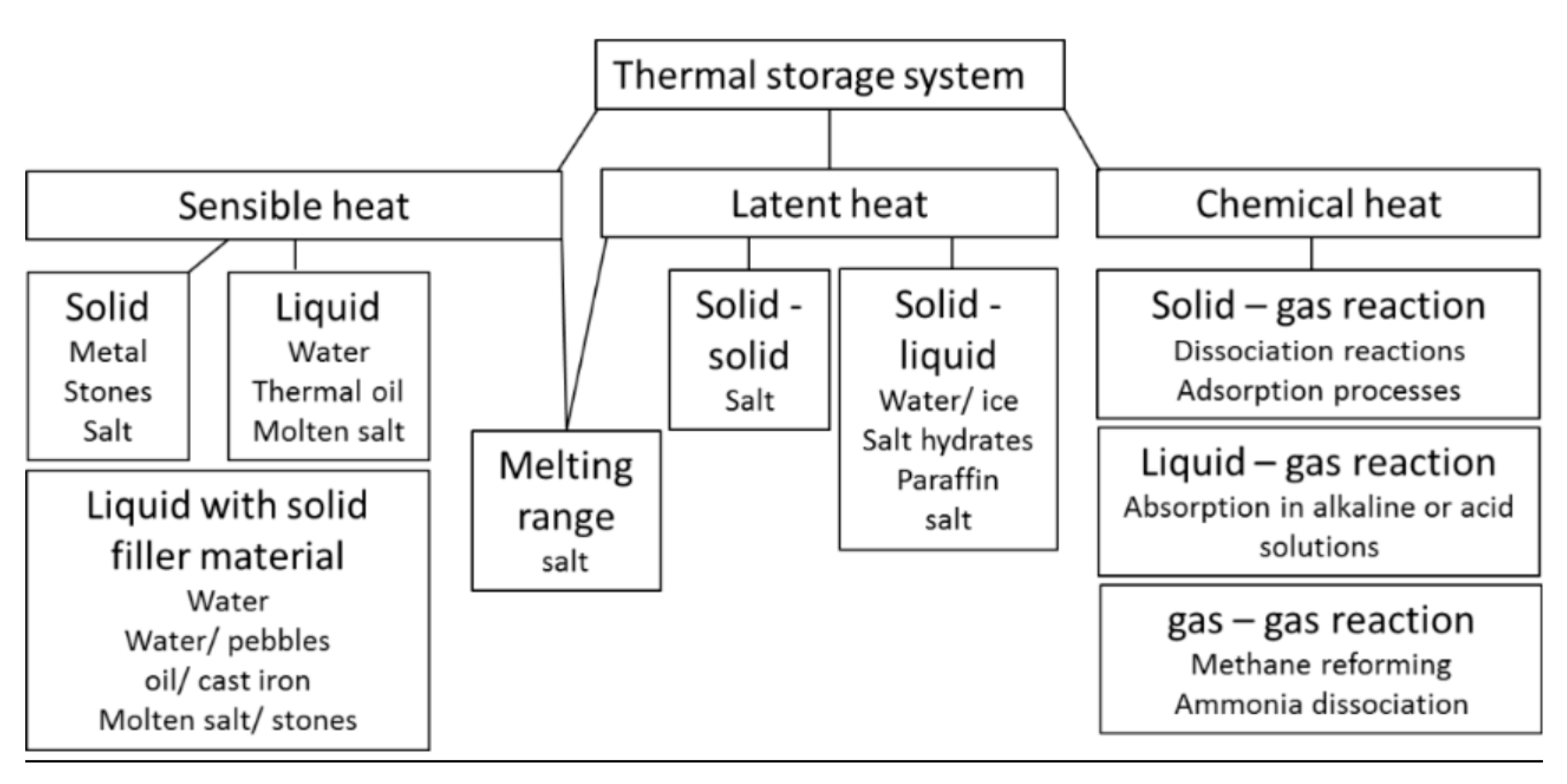
Similarly, in recent years, in small and medium enterprises, flywheels, flow batteries, fuel cells, thermal energy storage (TES), etc., have become imperative in the energy division. The rapid comeback through indicting and absolution marks them as beneficial for several short- and long-term solicitations, particularly in electrical superiority. In short, the energy productivity of extraordinary energy concentration and energy storing machinery, growing storing paybacks, solidity, dependability, energy preservation, and ecological sanctuary predictions are the major choices for cumulative energy requirements. Due to the proliferation in heat, thermal energy is produced due to the pileup of atoms and spots. TES philosophy is used in several arenas of biological disciplines. Essentially, there are three skills for TES. The graphical demonstration of TES techniques is given in Figure 1.

6.1. Sensible TEST

Sensible heat storage (SHS) is a structure of energy incorporated by growing or reducing the heat of the stored substance. This moderate storing is presented in a solid or liquid arrangement. Water is economical and one of the most frequently used mediums. The graphical demo of sensible TEST is displayed in Figure 2. Sensible thermal energy storage (STES) is extensively used in numerous mechanisms, for example, construction and solar power plants, as well as in solar preservation, solar food drying, and solar cuisine. STES is the easiest and most established method of heat storage. Sensible thermal energy (STE) is stowed by fluctuating the heat of STES ingredients, such as water, oil, rock beds, bricks, sand, or clay. There is no stage evolution through heat modifications in STES ingredients. SHS is tranquil to control and rationally exclusive. It is the best traditional, developed, and broadly used TES resolution. However, it accomplishes a minor energy-storing compactness than other TES alternatives, namely latent heat storage (LHS) and thermochemical heat storage (TCHS) [44]. In this process, the transference of energy to storing moderate liquors or solids clues to the identical alteration in the warmth of the medium. One of the benefits of this approach is that the storing and discharging of collected temperature (charge and discharge phases) can be repetitively deprived of difficulties, although accumulation of huge capacities can cause exceptions [45].
In addition, this scheme regularly receives the benefits of specific features of the stockpiled substantial, such as its particular high temperature [46]. Two core features of SHS ingredients must be tracked to raise capability storing ability (MJ• m 3 ) with extraordinary explicit temperature and compactness. Water has a moderately exceptional particular temperature and solidity among the abundant materials available, so it is frequently used to store substantial energy in numerous everyday uses. As for water with a thermal gradient of 60 °C, the SHS capability is assessed to be 250 MJ• m 3 [47]. This indicates that high thermal ratings expedite heat discharge, consenting to the transferal of low-temperature thermal energy to cooler areas during charging, consequential in a quicker approval of extraordinary power from the warmest site for the duration of expulsion. Temperature stream restrictions are essential variables that disturb thermal inertia in reflexive structure presentations [48]. This parameter designates the degree to which the substantial discharges or engages temperature, where its elevation increases heat storage and reduces energy depletion [49]. Furthermore, obtainability, budget, harmfulness, and capacity variations are advanced standards for picking justifiable SHS constituents. As stated, the core shortcomings are narrow energy compactness and device self-discharge. To estimate the recital of SHS schemes, Cardenas-Ramírez et al. [50] stated that the usable capacity is defined by energy storing ability, influence, productivity, charge/discharge cycle time, and budget.

6.2. Latent TEST

The LHS structure implicates storing energy in phase change materials (PCMs). Thermal energy is stored and unconfined when the storage material changes the segments. The benefit of LHS schemes is that these are usually condensed. For a particular heat-storing, the PCMs size is considerably slighter than the size of the SHS. This is essential since it affects the usage of fewer separations and is functional everywhere around the universe. Other compensations of PCMs include the capability to stock huge volumes of heat with minor temperature alterations and be pragmatic to severe operative temperatures since they can handle exertion under isothermal circumstances and have extraordinary storing compactness. Related to SHS schemes, LHS structures have almost 5 to 10 times greater storing solidity. The stage alteration can be from solid to liquid, solid to gas, solid to solid, liquid to gas, and vice versa. In solid-stage alteration, heat is stockpiled as the substantial transmission from one sparkler organization to another. This stage conversion, i.e., solid-to-solid alteration, has less latent heat. High latent heat issues and high capacity deviations are connected with solid-to-gas and liquid-to-gas transformation. However, considerable variations in size can be delinquent due to the requirement for a larger vessel. In several circumstances, this marks the method as other composite and unrealistic. For the causes stated formerly, the best superlative stage alteration is the transition from solid to liquid, as it is associated with minor changes in volume, although the latent heat of the solid–liquid growth is lesser than that of liquid to gas. Solid–liquid segment alteration substantial is also economical as thermal energy storing modes. PCM itself cannot be reused as a heat transmission mode. An isolated heat transmission cause should be retrieved, with a heat exchanger in the interior, to transfer energy from the basis to the PCM and PCM to the load. Assuming that PCM’s thermal dispersal is commonly small, consideration must be rewarded to the enterprise of temperature exchanger. Compared to SHS, LHS structures have a moderately surprising energy solidity and have existed for low- and medium-temperature presentations; for example, thermal contentment in constructions [51]. Thus, the perspective of excessive heat LHS structures desires to be assessed for incorporation with prodigious heat-concentrated solar power demonstrations. Low thermal conductivity, low thermal constancy, and restrained temperature of PCM sentimental in present LHS structures are critical barriers to their frame arrangement, even if they have significant energy-storing strengths. In customary concealed storage structures, there are different methods to progress thermal enactment through organs, flowing unlike PCMs and embalmed PCMs [52]. However, these approaches have the retention capacity bargain confines of PCMs, consequential in reducing the energy solidity capability through charging/discharge of the LHS scheme [53]. One viable substitute is metal PCMs with unusual thermal conductivity, sentimental warmth, and abundant thermal solidity. Generally, the melt’s latent heat and the mixture material’s thermal constancy rise with the growth in the soppy heat [54]. Hence, there is rising importance in educating PCMs through unexpected melting point heats.

6.3. Thermo-Chemical TEST

TCHS is one of the potential techniques of TES in the procedure of revocable thermochemical reactions. The main significant benefit of TCHS is that the enthalpy of the reaction is considerably more than the heat. Thus, the storing compactness is precisely superior. In organic responses, energy is stockpiled in biochemical bonds among molecules forming fragments. At the atomic level, energy storage contains energy related to the orbital of electrons. Besides whether the chemical captivates or discharges the reaction energy, there is no global modification in the quantity of energy through the reaction. The purpose of incorporating the TCES technique obsessed by the solar thermal system (STS) is to escalate the stake of solar energy and thus spread the productivity of the STS. The excess heat delivered by the summer stock accumulator arena controls the TCES. In the wintertime, stowed heat can be reprocessed to come across the excessive heat mandate of the structure. Conforming to the heat mandate of the structure and the extent of the TCHS, fossil-assisted STS using a proportion of more than 50% can be apprehended, and a pure STS can be esteemed. TCHS is linked to the water shield storing customary integrated STS over solar circuits and heat exchangers. The core component of TCHS is the heat and mass transfer that arises through the charge and discharge of the reactor. Dependent on the regulator policy, the reactor is premeditated as a fixed bed reactor. The substantial comes into the reactor from above, and passages over the reactor are determined by gravity. Air moves in the reactor and passages moisture and heat to and from the reactor. For air-to-air heat altercation, entering fresh air is heated by hot air departure TCHS. This controls the productivity of TCHS as heat damage by the gas stream is reduced. The heat unconfined in the reactor is transmitted from the airflow to the solar circuit via air-to-water heat exchange in TCHS release heating. For substantial preservation, the airflow is absorbed in the opposed way and reprocessed to transference reformative heat from the solar circuit to the reactor through the heat exchange airflow [55].
TCHS is used in a series of reactions related to physical and chemical developments. For a provisional organization, see [56]. In this organization, adsorption is used to accumulate various physical spectacles and can lead to misinterpretations. We deliberately limited organizational enlargement to diverse responses involving two extra steps, as TES rarely uses consistent responses. The priority of TEST is a critical enterprise in the current epoch. Industrial boldness is managed by reflection, economic strategies, and biological ideas of purpose and is often materially inadequate. The adequate sampling program selects the best TEST through an exciting presentation of the most viable economic proposal. Some unpredictable DM approaches have feasted the TEST. Basic DM methods should be adopted to remove these established doubts. We recommend using a specific modern CC-based TOPSIS method for useful IVIFHSNs. Careful consideration of the extension and DM identification described above can highlight all settings. It first focuses on TES techniques and then on weight inputs for multiple sub-parameters and other features to collect components from DM. Excellent exceptional structures are considered when choosing an operative TES method in DM. Selecting TEST main transmission surprises and attracts people to the logical order inherent in the tender. MADM contemplates framing decisions when presenting several conflicting standards. Each collection has different ranges, quality characteristics, and comparable weight components. Some processes can be systematically organized, while others can only be determined automatically. Many approaches can be used to designate MADM flaws. The MADM method adds to a lot of administrative complications. This study’s main neutrality is choosing the most appropriate TEST for the correlation-based TOPSIS technique in the IVIFHSS setting.

6.4. Numerical Example

Suppose H = H 1 , H 2 , H 3 is a collection of alternatives such that: H 1 : Latent TEST, H 2 : Sensible TEST, 3 : Thermochemical TEST, and Ϛ = ϛ 1 , ϛ 2 , ϛ 3 , ϛ 4 are the set of criteria. Let H = H 1 , H 2 , H 3 be a group of professionals with weights 0.3 , 0.4 , 0.3 T . Experts considered the parameters for the selection of the finest TEST, such as: ϛ 1 = Energy storage capacity, ϛ 2 = Efficiency, ϛ 3 = minimum cycle length. The multi sub-attributes of the pondered aspects are: Energy storage capacity = ϛ 1 = ϛ 11 = H e a t   s t o r e d   i n   t h e   m a t e r i a l ,   ϛ 12 = H e a t   s t o r e d   i n   t h e   c o m p o n e n t s   o f   t h e   s y s t e m , Efficiency = ϛ 2 = ϛ 21 = h e a t   r e l e a s e d   t o   t h e   h e a t   s i n k   d u r i n g   d i s c h a r g i n g ,   ϛ 22 = e n e r g y   a b s o r b e d   b y   t h e   s y s t e m   d u r i n g   c h a r g i n g , Minimum cycle length = ϛ 3 = ϛ 31 = s h o r t   t e r m ,   ϛ 32 = l o n g   t e r m . Let Ϛ = ϛ 1 × ϛ 2 × ϛ 3 be a set of sub-attributes. Then
Ϛ = ϛ 1 × ϛ 2 × ϛ 3 = ϛ 11 , ϛ 12 × ϛ 21 , ϛ 22 × ϛ 31 , ϛ 32 = ϛ 11 , ϛ 21 , ϛ 31 , ϛ 11 , ϛ 21 , ϛ 32 , ϛ 11 , ϛ 22 , ϛ 31 , ϛ 11 , ϛ 22 , ϛ 32 , ϛ 12 , ϛ 21 , ϛ 31 , ϛ 12 , ϛ 21 , ϛ 32 , ϛ 12 , ϛ 22 , ϛ 31 , ϛ 12 , ϛ 22 , ϛ 32
Let Ϛ = ϛ ˇ 1 , ϛ ˇ 2 , ϛ ˇ 3 , ϛ ˇ 4 , ϛ ˇ 5 , ϛ ˇ 6 , ϛ ˇ 7 , ϛ ˇ 8 be a collection of multi-sub-attributes with weights γ j = 0.1 , 0.2 , 0.05 , 0.15 , 0.05 , 0.15 , 0.12 , 0.18 T . Professionals provide preferences for each alternative in the IVIFHSN form because of considered aspects. The expert group commented on each option in Table 1, Table 2 and Table 3 below as IVIFHSN. The TOPSIS-based MADM problem was introduced in Section 5 to find the most appropriate TEST.
Step 1. Development of decision matrices for alternatives H = H 1 , H 2 , H 3 , H 4 in the form of IVIFHSNs under-considered attributes given as Table 1, Table 2 and Table 3.
Step 2: The considered parameters are all the same types, meaning there are no different sub-parameters. Thus, no need to normalize.
Step 3: Construction of a weighted decision matrix for each alternative H ( z ) = Δ ϛ i j ^ ( z ) n × ρ given in Table 4, Table 5 and Table 6.
Step 4. Employment of Equations (15) and (16) to compute the PIA and NIA, respectively.
Δ ϛ i j ^ ( z ) + = 0.0437 , 0.0588 , 0.8686 , 0.9229 0.0220 , 0.0424 , 0.9443 , 0.9576 0.0127 , 0.0226 , 0.9703 , 0.9774 0.0564 , 0.0741 , 0.9721 , 0.9869 0.0588 , 0.0770 , 0.8686 , 0.9000 0.0220 , 0.0314 , 0.9443 , 0.9686 0.0127 , 0.0172 , 0.9703 , 0.9828 0.0264 , . 00507 , 0.9336 , 0.9493 0.0247 , 0.0351 , 0.9379 , 0.9649 0.0053 , 0.0177 , 0.9416 , 0.9823 0.0071 , 0.0102 , 0.9683 , 0.9862 0.0063 , 0.0133 , 0.9698 , 0.9867 0.0247 , 0.0474 , 0.9379 , 0.9526 0.0111 , 0.0252 , 0.9552 , 0.9659 0.0182 , 0.0317 , 0.9549 , 0.9683 0.0063 , 0.0133 , 0.9788 , 0.9867 0.0265   0.0469 , 0.9189 , 0.9387 0.0133 , 0.0189 , 0.9662 , 0.9743 0.0033 , 0.0053 , 0.9661 , 0.9924 0.0047 , 0.0099 , 0.9841 , 0.9900 0.0469   0.0613 , 0.9189 , 0.9387 0.0189 , 0.0257 , 0.9559 , 0.9662 0.0103 , 0.0179 , 0.9661 , 0.9821 0.0047 , 0.0099 , 0.9693 , 0.9900
Δ ϛ i j ^ ( z ) = 0.0564 , 0.0741 , 0.4721 , 0.5169 0.0265 , 0.0345 , 0.4935 , 0.5467 0.0256 , 0.0645 , 0.4835 , 0.5467 0.0342 , 0.0477 , 0.5134 , 0.5348 0.0127 , 0.0253 , 0.5134 , 0.5248 0.0264 , 0.0541 , 0.4721 , 0.5169 0.0464 , 0.0541 , 0.4921 , 0.5061 0.0356 , 0.0545 , 0.4735 , 0.5267 0.0174 , 0.0539 , 0.6945 , 0.7962 0.0235 , 0.0497 , 0.5863 , 0.6771 0.0512 , 0.0576 , 0.6163 , 0.6260 0.0572 , 0.0676 , 0.5863 , 0.5960 0.0235 , 0.0397 , 0.5963 , 0.6171 0.0472 , 0.0476 , 0.5763 , 0.5860 0.0472 , 0.0576 , 0.5763 , 0.5960 0.0294 , 0.0537 , 0.6149 , 0.6578 0.0253 , 0.0357 , 0.5309 , 0.5385 0.0142 , 0.0249 , 0.5267 , 0.6172 0.0236 , 0.0361 , 0.6152 , 0.6232 0.0136 , 0.0561 , 0.6352 , 0.6532 0.0436 , 0.0583 , 0.6256 , 0.6435 0.0153 , 0.0357 , 0.5709 , 0.6385 0.0253 , 0.0357 , 0.5809 , 0.6085 0.0142 , 0.0549 , 0.5867 , 0.6872
Step 5. Calculate the CC between H ( z ) and PIA Δ ϛ i j ^ ( z ) + using Equation (17).
κ ( 1 ) = 0.99157 ,   κ ( 2 ) = 0.99537 ,   κ ( 3 ) = 0.99142
Step 6. Calculate the CC between H ( z ) and PIA Δ ϛ i j ^ ( z ) using Equation (18).
τ ( 1 ) = 0.99572 ,   τ ( 2 ) = 0.99344 ,   τ ( 3 ) = 0.99562
Step 7. Use Equation (19). to find the closeness coefficient.
( 1 ) = 0.66326 ,   ( 2 ) = 0.41749 ,   ( 3 ) = 0.66204
Step 8. The maximum value of the closeness coefficient shows that ( 1 ) is the finest TEST.
Step 9. Therefore, the ranking of the alternatives is H ( 1 ) > H ( 3 ) > H ( 2 ) .

7. Discussion and Comparative Analysis

The consequent section compares the presented method and prevalent approaches to consent to the pragmatism of the conveyed structure.

7.1. Supremacy of the Planned Approach

The planned methodology is brilliant and significant. We present a correlation-based TOPSIS method to explicate MADM obstacles under IVIFHSS. The method established in this study is more exact than the predominant approaches, and its compatibility deals with MADM concerns. The delivered technique is multipurpose and conversant, providing for different results with disparity, culpability, and modification. For different replicas with precise classification characteristics, general changes are made to the estimate structure, ordered to compete with their point of view. Organizational studies and approximations show that prevailing methodologies’ results are comparable to those of hybrids. In addition, several amalgam configurations of FS and IFS convert into the exceptional circumstances of IVIFHSS by accumulating particular environments. Object-related facts can be designated in a specific and tentative way (see Table 7), and it is a reasonably suitable tool for combining inaccurate and inexact statistics in DM agendas. Over this study and assessment, we have noted that the proposed method’s results are more general than any presented structure. However, the anticipated DM development comprises an enormous expanse of facts to release concern in the statistics relative to the proposed DM techniques. Thus, the anticipated scheme is operative, supple, and expedient, and superior to other FS and IFS hybrid configurations. In addition, when adding some proper rapports, several amalgamation formations of IVFS turn into IVIFHSS. Adding unusual and vague realities to the current real package is surprising. Here, facts about well-being can be designated thoroughly and realistically. Over the DM process, fictional and disconcerting facts are collective. Thus, our planned scheme would be better, momentous, extraordinary, and multiple combination FS circumstances. Table 7 shows the characteristics of our settled and prevalent methods. The ✓ and × represents the yes and no respectively.
This is a recent delinquent. Why do we want to represent an innovative TOPSIS method built on the anticipated organization? There are numerous displays associated with other prevailing techniques. The planned methodology might be an exception. The hybrid structure boundaries FS, IVFS, IFS, IVIFS, FSS, IVFSS, IFSS, IVIFSS, and IFHSS cannot deliver thorough details about the situation. However, our developed correlation-based TOPSIS method for IVIFHSS can handle the sub-attributes considering the MD and NMD. Other TOPSIS methods of existing hybrid structures are reduced into IVIFHSS configuration. Table 7 above presents the supremacy of our proposed hybrid structure of FS and shows that it has a great perspective over prevailing hybrid systems of FS.

7.2. Comparative Studies

The above general research and comparative studies show that the results of the adopted methods overlap with the available techniques, so the developed correlation-based TOPSIS method is conformist. However, collectively with nearby DM methods, the core advantage of the designed TOPSIS model is that it adjusts extra information considering the sub-parameters of the alternatives to contracting with vagueness in the data. Object-related facts can be described more clearly and empirically, and it is also a beneficial tool for determining inexact and inexplicable facts in the DM procedure. Moreover, it can be seen from comparative analysis that the intention progression of the scheduling technique is not the same because of the PIA and NIA commitment. In previous methods, PIA and NIA were intellectualized based on distance and similarity measures. Thus, encouragement for the score value qualified to each parameter does not mark other parameters, so there is an estimated loss of facts in the progression. Meanwhile, in the planned scheme, PIA and NIA are considered based on determining CC enticement at a given substitute level, so there is no severe loss of facts in the procedure. The power of each ideal correlation measure is derived from revising the clarifications to determine the most advanced consequences and determine the correlation among them. The benefit of the intentional TOPSIS technique over recent techniques and correlated measures is that it precedes communication of not only the degree of perception but also the degree of similarity among clarifications, therefore circumventing conclusions built on destructive bases. Finally, the abundance of all alternatives by the existing TOPSIS methods contributes to the same final judgment to select H ( 1 ) TEST. Cavallaro’s [4] fuzzy TOPSIS and Ashtiani et al.’s [8] IVFS TOPSIS only contract the MD of alternatives in fuzzy and interval-valued fuzzy numbers, respectively. Rouyendegh et al.’s [10] IFS TOPSIS and Zhang and Yu’s [17] IVIFS TOPSIS approaches handle the alternatives ranking considering the MD and NMD. However, these TOPSIS methodologies cannot deal with the parametrization of alternatives. Similarly, the TOPSIS method established by Garg and Arora [25] and Zulqarnain et al. [29] under IFSS and IVIFSS cannot solve the multi-sub-attributes of the alternatives. The TOPSIS method developed in [39] handled the alternatives’ sub-attributes but ignored the information in intervals form. On the other hand, the aggregation operators designed in [41] and interval-valued intuitionistic fuzzy hypersoft interactive weighted average aggregation operator [42] capably deal with the drawbacks mentioned above under the IVIFHSS setting. However, in some particular circumstances, these aggregation operators also failed to handle the abovementioned concerns. Meanwhile, our proposed TOPSIS model expertly deals with these concerns. The comparison results are enumerated below (see Table 8), with the final ranking of the top 3 alternatives. The results show that the optimal choice of the planned technique is symmetric with the prevalent method, demonstrating the projected technique’s consistency and efficiency.

7.3. Merits and Theoretical Advantages of the Proposed Model

The planned model is better and more reliable due to the following aspects:
Experts’ choice of attributes and classification based on sub-attributes is not continually absolute in several conditions. Experts faced different reservations in this worry. The model developed in this research solves this state utilizing the notion of interval-valued intuitionistic fuzzy parametrization that determines the unpredictable behavior of attributes and their sub-attributes.
The scheduled TOPSIS model supports the experts to provide their estimates based on 2D MD and NMD functions, allowing them to agree or disagree with estimations individually in intervals form.
It is generally determined that the predicted values of the attributes and their sub-attributes can match to elucidate the hesitation. The offered model explains these matching values by seeing 2D MD and NMD functions in intervals form, which uses stage values to compact with duplications initiated on this data.
Providing an estimate built on a single parameter is an inefficient procedure. The projected TOPSIS model supports the experts in delivering their assessments considering sub-attributes in the HSS environment.
This study’s mathematical clarifications of correlation coefficients approve the developed scheme’s symmetry, indicating that the proposed algorithm is well-balanced and exhibits no biases or irregularities. This relationship with symmetry is important as it ensures that the proposed algorithm is fair and reliable in its DM process. It also suggests that the algorithm can be used in various applications where symmetry and balance are essential for accurate decisions.
The study’s focus on IVIFHSS represents a significant theoretical advancement, as it is the most generalized form of interval-valued intuitionistic fuzzy soft sets. The development of informational energies for IVIFHSS settings and the discussion of their elementary properties further advance the theoretical framework for IVIFHSS.
Overall, the study contributes to developing more reliable and accurate approaches to DM in the context of IVIFHSS and represents an essential theoretical advancement in fuzzy sets and decision-making.

8. Conclusions

This study focuses on IVIFHSS to address concerns of inadequate data, obscurity, and irregularity by seeing the MD and NMD values of n-tuple sub-attributes of the deliberated attributes. The fundamental objective of this study is to introduce novel correlation measures for IVIFHSS, such as CC and WCC. Several characteristics of these measures have also been studied in detail. By design only one parameter in the exploration and numerous prevailing correlation measures in the perspective of an IFS can be deliberated as distinctive circumstances of the planned measures. Based on settled CC and WCC, the TOPSIS technique is presented by considering the sub-attributes and experts to resolve MADM hurdles, and determining the correlation indices and closeness coefficient to find the PIA (NIA) and rank of alternatives, respectively. To distinguish the effects of the intended TOPSIS technique, we provided a numerical illustration for choosing a thermal energy storage technique. Moreover, a comparative analysis is conceded to sanction and symmetry of the method’s efficacy and perfect nature. Lastly, based on the outcomes attained, it can be determined that the anticipated technique has extraordinary constancy and concrete capability for decision-makers in the DM procedure. Future studies will recommend VIKOR and MABAC methods to report DM concerns. Moreover, several other aggregation operators can be developed, such as Bonferroni Mean AOs, Einstein AOs, Einstein ordered AOs, Einstein hybrid AOs, etc., along with their applications in real-life problems. This includes potential applications in various fields such as engineering, management, medical sciences, and social sciences, where decision-making under uncertainty and imprecise information is critical.

Author Contributions

Conceptualization, R.M.Z. and W.-X.M.; methodology, W.-X.M.; software, I.S.; validation, I.S. and A.A.; formal analysis, A.A. and H.A.E.-W.K.; investigation, R.M.Z. and H.A.E.-W.K.; resources, I.S.; data curation, R.M.Z.; writing—original draft preparation, R.M.Z. and I.S.; writing—review and editing, R.M.Z. and A.M.A.; visualization, A.M.A.; supervision, W.-X.M.; project administration, W.-X.M.; funding acquisition, R.M.Z., A.M.A. All authors have read and agreed to the published version of the manuscript.

Data Availability Statement

Not applicable.

Acknowledgments

The researchers would like to thank the Deanship of Scientific Research, Qassim University for funding the publication of this project.

Conflicts of Interest

The authors declare no conflict of interest.

References

  1. Dincer, I. Thermal energy storage systems as a key technology in energy conservation. Int. J. Energy Res. 2002, 26, 567–588. [Google Scholar] [CrossRef]
  2. Koçak, B.; Fernandez, A.I.; Paksoy, H. Review on sensible thermal energy storage for industrial solar applications and sustainability aspects. Sol. Energy 2020, 209, 135–169. [Google Scholar] [CrossRef]
  3. Zadeh, L.A. Fuzzy Sets. Inf. Control 1965, 8, 338–353. [Google Scholar] [CrossRef] [Green Version]
  4. Cavallaro, F. Fuzzy TOPSIS approach for assessing thermal-energy storage in concentrated solar power (CSP) systems. Appl. Energy 2010, 87, 496–503. [Google Scholar] [CrossRef]
  5. Turksen, I.B. Interval valued fuzzy sets based on normal forms. Fuzzy Sets Syst. 1986, 20, 191–210. [Google Scholar] [CrossRef]
  6. Yu, C. Correlation of fuzzy numbers. Fuzzy Sets Syst. 1993, 55, 303–307. [Google Scholar] [CrossRef]
  7. Pekaslan, D.; Wagner, C.; Garibaldi, J.M. Adonis—Adaptive online nonsingleton fuzzy logic systems. IEEE Trans. Fuzzy Syst. 2019, 28, 2302–2312. [Google Scholar] [CrossRef]
  8. Ashtiani, B.; Haghighirad, F.; Makui, A.; ali Montazer, G. Extension of fuzzy TOPSIS method based on interval-valued fuzzy sets. Appl. Soft Comput. 2009, 9, 457–461. [Google Scholar] [CrossRef]
  9. Atanassov, K.T. Intuitionistic fuzzy sets. In Intuitionistic Fuzzy Sets; Physica-Verlag HD: Heidelberg, Germany, 1999; pp. 1–137. [Google Scholar]
  10. Rouyendegh, B.D.; Yildizbasi, A.; Üstünyer, P. Intuitionistic fuzzy TOPSIS method for green supplier selection problem. Soft Comput. 2020, 24, 2215–2228. [Google Scholar] [CrossRef]
  11. Atanassov, K.T. Interval Valued Intuitionistic Fuzzy Sets. In Intuitionistic Fuzzy Sets; Studies in Fuzziness and Soft Computing; Physica-Verlag HD: Heidelberg, Germany, 1999; Volume 35. [Google Scholar] [CrossRef]
  12. Tang, Y.M.; Zhang, L.; Bao, G.Q.; Ren, F.J.; Pedrycz, W. Symmetric implicational algorithm derived from intuitionistic fuzzy entropy. Iran. J. Fuzzy Syst. 2022, 19, 27–44. [Google Scholar]
  13. Hung, W.L.; Wu, J.W. Correlation of intuitionistic fuzzy sets by centroid method. Inf. Sci. 2002, 144, 219–225. [Google Scholar] [CrossRef]
  14. Bustince, H.; Burillo, P. Correlation of interval-valued intuitionistic fuzzy sets. Fuzzy Sets Syst. 1995, 74, 237–244. [Google Scholar] [CrossRef]
  15. Hong, D.H. A note on correlation of interval-valued intuitionistic fuzzy sets. Fuzzy Sets Syst. 1998, 95, 113–117. [Google Scholar] [CrossRef]
  16. Mitchell, H. A correlation coefficient for intuitionistic fuzzy sets. Int. J. Intell. Syst. 2004, 19, 483–490. [Google Scholar] [CrossRef]
  17. Zhang, H.; Yu, L. MADM method based on cross-entropy and extended TOPSIS with interval-valued intuitionistic fuzzy sets. Knowl.-Based Syst. 2012, 30, 115–120. [Google Scholar] [CrossRef]
  18. Jana, C.; Muhiuddin, G.; Pal, M.; Al-Kadi, D. Intuitionistic fuzzy dombi hybrid decision-making method and their applications to enterprise financial performance evaluation. Math. Probl. Eng. 2021, 2021, 3218133. [Google Scholar] [CrossRef]
  19. Paul, T.K.; Jana, C.; Pal, M.; Simic, V. Sustainable carbon-dioxide storage assessment in geological media using modified Pythagorean fuzzy VIKOR and DEMATEL approach. Int. J. Hydrog. Energy 2022, 48, 9474–9497. [Google Scholar] [CrossRef]
  20. Jana, C.; Muhiuddin, G.; Pal, M. Some Dombi aggregation of Q-rung orthopair fuzzy numbers in multiple-attribute decision making. Int. J. Intell. Syst. 2019, 34, 3220–3240. [Google Scholar] [CrossRef]
  21. Singh, S.; Sharma, S.; Lalotra, S. Generalized correlation coefficients of intuitionistic fuzzy sets with application to MAGDM and clustering analysis. Int. J. Fuzzy Syst. 2020, 22, 1582–1595. [Google Scholar] [CrossRef]
  22. Molodtsov, D. Soft set theory—First results. Comput. Math. Appl. 1999, 37, 19–31. [Google Scholar] [CrossRef] [Green Version]
  23. Maji, P.K.; Biswas, R.; Roy, A.R. Fuzzy soft sets. J. Fuzzy Math. 2001, 9, 589–602. [Google Scholar]
  24. Maji, P.K.; Biswas, R.; Roy, A.R. Intuitionistic fuzzy soft sets. J. Fuzzy Math. 2001, 9, 677–692. [Google Scholar]
  25. Garg, H.; Arora, R.; Arora, R. TOPSIS method based on correlation coefficient for solving decision-making problems with intuitionistic fuzzy soft set information. AIMS Math. 2020, 5, 2944–2966. [Google Scholar] [CrossRef]
  26. Jiang, Y.; Tang, Y.; Chen, Q.; Liu, H.; Tang, J. Interval-valued intuitionistic fuzzy soft sets and their properties. Comput. Math. Appl. 2010, 60, 906–918. [Google Scholar] [CrossRef] [Green Version]
  27. Ma, X.; Qin, H.; Abawajy, J. Interval-valued intuitionistic fuzzy soft sets based decision making and parameter reduction. IEEE Trans. Fuzzy Syst. 2020, 30, 357–369. [Google Scholar] [CrossRef]
  28. Khan, M.J.; Kumam, P.; Liu, P.; Kumam, W. Another view on generalized interval valued intuitionistic fuzzy soft set and its applications in decision support system. J. Intell. Fuzzy Syst. 2020, 38, 4327–4341. [Google Scholar] [CrossRef]
  29. Zulqarnain, R.M.; Xin, X.L.; Saqlain, M.; Khan, W.A. TOPSIS method based on the correlation coefficient of interval-valued intuitionistic fuzzy soft sets and aggregation operators with their application in decision-making. J. Math. 2021, 2021, 6656858. [Google Scholar] [CrossRef]
  30. Garg, H.; Arora, R. A nonlinear-programming methodology for multi-attribute decision-making problem with interval-valued intuitionistic fuzzy soft sets information. Appl. Intell. 2018, 48, 2031–2046. [Google Scholar] [CrossRef]
  31. Zulqarnain, M.; Saeed, M. A new decision making method on interval valued fuzzy soft matrix (IVFSM). Br. J. Math. Comput. Sci. 2017, 20, 1–17. [Google Scholar] [CrossRef]
  32. Zulqarnain, M.; Saeed, M. An application of interval valued fuzzy soft matrix (ivfsm) in decision making. Sci. Int. 2016, 28, 2261–2264. [Google Scholar]
  33. Zulqarnain, M.; Saeed, M.; Tabassum, M.F. Comparison between fuzzy soft matrix (fsm) and interval valued fuzzy soft matrix (ivfsm) in decision making. Sci. Int. 2016, 28, 4277–4283. [Google Scholar]
  34. Dayan, F.; Zulqarnain, M. On generalized interval valued fuzzy soft matrices. Am. J. Math. Comput. Model. 2018, 3, 1–9. [Google Scholar] [CrossRef] [Green Version]
  35. Smarandache, F. Extension of soft set to hypersoft set, and then to plithogenic hypersoft set. Neutrosophic Sets Syst. 2018, 22, 168–170. [Google Scholar]
  36. Rahman, A.U.; Saeed, M.; Khalifa, H.A.E.W.; Afifi, W.A. Decision making algorithmic techniques based on aggregation operations and similarity measures of possibility intuitionistic fuzzy hypersoft sets. AIMS Math. 2022, 7, 3866–3895. [Google Scholar] [CrossRef]
  37. Rahman, A.U.; Saeed, M.; Garg, H. An innovative decisive framework for optimized agri-automobile evaluation and HRM pattern recognition via possibility fuzzy hypersoft setting. Adv. Mech. Eng. 2022, 14, 16878132221132146. [Google Scholar] [CrossRef]
  38. Zulqarnain, R.M.; Siddique, I.; Ali, R.; Pamucar, D.; Marinkovic, D.; Bozanic, D. Robust Aggregation Operators for Intuitionistic Fuzzy Hypersoft Set With Their Application to Solve MCDM Problem. Entropy 2021, 23, 688. [Google Scholar] [CrossRef]
  39. Zulqarnain, R.M.; Xin, X.L.; Saeed, M. Extension of TOPSIS method under intuitionistic fuzzy hypersoft environment based on correlation coefficient and aggregation operators to solve decision making problem. AIMS Math. 2020, 6, 2732–2755. [Google Scholar] [CrossRef]
  40. Debnath, S. Interval-Valued Intuitionistic Hypersoft Sets and Their Algorithmic Approach in Multi-criteria Decision Making. Neutrosophic Sets Syst. 2022, 48, 226–250. [Google Scholar]
  41. Zulqarnain, R.M.; Siddique, I.; Jarad, F.; Iampan, A. Aggregation Operators for Interval-Valued Intuitionistic Fuzzy Hypersoft Set with Their Application in Material Selection. Math. Probl. Eng. 2022. [Google Scholar] [CrossRef]
  42. Zulqarnain, R.M.; Siddique, I. An MCGDM Technique for Weighted Average Interaction Aggregation Operator Under Interval-Valued Intuitionistic Fuzzy Hypersoft Set Environment. J. Comput. Cogn. Eng. 2022. [Google Scholar] [CrossRef]
  43. Hwang, C.L.; Yoon, K. Methods for multiple attribute decision making. In Multiple Attribute Decision Making; Springer: Berlin/Heidelberg, Germany, 1981; pp. 58–191. [Google Scholar]
  44. Zhao, Y.; Zhao, C.Y.; Markides, C.N.; Wang, H.; Li, W. Medium-and high-temperature latent and thermochemical heat storage using metals and metallic compounds as heat storage media: A technical review. Appl. Energy 2020, 280, 115950. [Google Scholar] [CrossRef]
  45. Chandel, S.S.; Agarwal, T. Review of current state of research on energy storage, toxicity, health hazards and commercialization of phase changing materials. Renew. Sustain. Energy Rev. 2017, 67, 581–596. [Google Scholar] [CrossRef]
  46. Rathore, P.K.S.; Shukla, S.K. Potential of macroencapsulated PCM for thermal energy storage in buildings: A comprehensive review. Constr. Build. Mater. 2019, 225, 723–744. [Google Scholar] [CrossRef]
  47. Lizana, J.; Chacartegui, R.; Barrios-Padura, A.; Valverde, J.M. Advances in thermal energy storage materials and their applications towards zero energy buildings: A critical review. Appl. Energy 2017, 203, 219–239. [Google Scholar] [CrossRef]
  48. Borri, E.; Tafone, A.; Zsembinszki, G.; Comodi, G.; Romagnoli, A.; Cabeza, L.F. Recent trends on liquid air energy storage: A bibliometric analysis. Appl. Sci. 2020, 10, 2773. [Google Scholar] [CrossRef]
  49. Tarragona, J.; de Gracia, A.; Cabeza, L.F. Bibliometric analysis of smart control applications in thermal energy storage systems. A model predictive control approach. J. Energy Storage 2020, 32, 101704. [Google Scholar] [CrossRef]
  50. Cardenas-Ramírez, C.; Jaramillo, F.; Gomez, M. Systematic review of encapsulation and shape-stabilization of phase change materials. J. Energy Storage 2020, 30, 101495. [Google Scholar] [CrossRef]
  51. De Gracia, A.; Cabeza, L.F. Phase change materials and thermal energy storage for buildings. Energy Build. 2015, 103, 414–419. [Google Scholar] [CrossRef] [Green Version]
  52. Jegadheeswaran, S.; Pohekar, S.D. Performance enhancement in latent heat thermal storage system: A review. Renew. Sustain. Energy Rev. 2009, 13, 2225–2244. [Google Scholar] [CrossRef]
  53. Lin, Y.; Jia, Y.; Alva, G.; Fang, G. Review on thermal conductivity enhancement, thermal properties and applications of phase change materials in thermal energy storage. Renew. Sustain. Energy Rev. 2018, 82, 2730–2742. [Google Scholar] [CrossRef]
  54. Bauer, T.; Steinmann, W.-D.; Laing, D.; Tamme, R. Thermal Energy Storage Materials and Systems. Annu. Rev. Heat Transf. 2012, 15, 131–177. [Google Scholar] [CrossRef]
  55. Mette, B.; Kerskes, H.; Drück, H.; Badenhop, T.; Salg, F.; Gläser, R. Thermochemical energy storage as an element for the energy turnaround. In Proceedings of the International Renewable Energy Storage Conference, Berlin, Germany, 18–20 November 2013. [Google Scholar]
  56. McNaught, A.D.; Wilkinson, A. IUPAC Compendium of Chemical Terminology, 2nd ed.; Wiley Blackwell: Hoboken, NJ, USA, 1997. [Google Scholar]
Figure 2. Sensible Thermal Energy Storage Technique.
Symmetry 15 00615 g002
Table 1. Expert’s opinion for H 1 in IVIFHSNs.
ϛ ˇ 1 ϛ ˇ 2 ϛ ˇ 3 ϛ ˇ 4 ϛ ˇ 5 ϛ ˇ 6 ϛ ˇ 7 ϛ ˇ 8
H 1 0.4 , 0.5 , 0.2 , 0.5 0.3 , 0.6 , 0.1 , 0.3 0.4 , 0.6 , 0.2 , 0.4 0.2 , 0.3 , 0.2 , 0.5 0.3 , 0.6 , 0.1 , 0.3 0.3 , 0.5 , 0.2 , 0.5 0.4 , 0.5 , 0.2 , 0.5 0.2 , 0.4 , 0.2 , 0.6
H 2 0.2 , 0.5 , 0.2 , 0.4 0.2 , 0.4 , 0.4 , 0.5 0.2 , 0.3 , 0.4 , 0.6 0.2 , 0.6 , 0.2 , 0.4 0.2 , 0.5 , 0.2 , 0.4 0.2 , 0.5 , 0.1 , 0.4 0.2 , 0.3 , 0.2 , 0.6 0.2 , 0.3 , 0.4 , 0.7
H 3 0.3 , 0.5 , 0.1 , 0.4 0.4 , 0.6 , 0.2 , 0.3 0.4 , 0.7 , 0.3 , 0.3 0.3 , 0.5 , 0.1 , 0.4 0.1 , 0.5 , 0.1 , 0.4 0.3 , 0.5 , 0.1 , 0.4 0.3 , 0.5 , 0.1 , 0.4 0.3 , 0.6 , 0.2 , 0.4
Table 2. Expert’s opinion for H 2 in IVIFHSNs.
ϛ ˇ 1 ϛ ˇ 2 ϛ ˇ 3 ϛ ˇ 4 ϛ ˇ 5 ϛ ˇ 6 ϛ ˇ 7 ϛ ˇ 8
H 1 0.1 , 0.3 , 0.2 , 0.5 0.2 , 0.6 , 0.1 , 0.4 0.2 , 0.4 , 0.2 , 0.5 0.1 , 0.3 , 0.3 , 0.5 0.3 , 0.5 , 0.2 , 0.3 0.1 , 0.4 , 0.2 , 0.5 0.1 , 0.5 , 0.2 , 0.4 0.1 , 0.3 , 0.2 , 0.6
H 2 0.2 , 0.4 , 0.2 , 0.4 0.2 , 0.3 , 0.1 , 0.5 0.2 , 0.4 , 0.4 , 0.5 0.2 , 0.5 , 0.2 , 0.4 0.2 , 0.4 , 0.3 , 0.5 0.2 , 0.3 , 0.1 , 0.6 0.2 , 0.3 , 0.2 , 0.6 0.2 , 0.4 , 0.4 , 0.5
H 3 0.3 , 0.5 , 0.1 , 0.3 0.4 , 0.5 , 0.2 , 0.4 0.1 , 0.3 , 0.3 , 0.6 0.3 , 0.4 , 0.1 , 0.5 0.1 , 0.3 , 0.1 , 0.4 0.3 , 0.5 , 0.1 , 0.3 0.3 , 0.5 , 0.1 , 0.4 0.3 , 0.5 , 0.2 , 0.4
Table 3. Expert’s opinion for H 3 in IVIFHSNs.
ϛ ˇ 1 ϛ ˇ 2 ϛ ˇ 3 ϛ ˇ 4 ϛ ˇ 5 ϛ ˇ 6 ϛ ˇ 7 ϛ ˇ 8
H 1 0.2 , 0.5 , 0.2 , 0.4 0.2 , 0.6 , 0.1 , 0.3 0.2 , 0.5 , 0.2 , 0.4 0.2 , 0.6 , 0.2 , 0.3 0.3 , 0.5 , 0.1 , 0.3 0.1 , 0.5 , 0.2 , 0.4 0.2 , 0.4 , 0.1 , 0.5 0.2 , 0.4 , 0.2 , 0.5
H 2 0.2 , 0.5 , 0.2 , 0.3 0.2 , 0.5 , 0.2 , 0.4 0.2 , 0.4 , 0.4 , 0.5 0.2 , 0.5 , 0.2 , 0.4 0.2 , 0.4 , 0.2 , 0.5 0.2 , 0.4 , 0.1 , 0.5 0.1 , 0.3 , 0.2 , 0.4 0.2 , 0.3 , 0.4 , 0.6
H 3 0.1 , 0.4 , 0.2 , 0.4 0.3 , 0.7 , 0.2 , 0.3 0.4 , 0.6 , 0.3 , 0.4 0.3 , 0.4 , 0.1 , 0.5 0.1 , 0.3 , 0.1 , 0.6 0.3 , 0.4 , 0.1 , 0.5 0.3 , 0.5 , 0.3 , 0.4 0.3 , 0.5 , 0.2 , 0.4
Table 4. Weighted decision matrix for H ( 1 ) .
ϛ ˇ 1 ϛ ˇ 2 ϛ ˇ 3 ϛ ˇ 4 ϛ ˇ 5 ϛ ˇ 6 ϛ ˇ 7 ϛ ˇ 8
H 1 0.0564 , 0.0741 , 0.4721 , 0.5169 0.0127 , 0.0453 , 0.5134 , 0.5348 0.0256 , 0.0645 , 0.4835 , 0.5467 0.0342 , 0.0477 , 0.5134 , 0.5348 0.0127 , 0.0443 , 0.5374 , 0.5648 0.0264 , 0.0541 , 0.4721 , 0.5169 0.0342 , 0.0477 , 0.5234 , 0.5748 0.0356 , 0.0545 , 0.4735 , 0.5267
H 2 0.0174 , 0.0539 , 0.6945 , 0.7962 0.0235 , 0.0497 , 0.5863 , 0.6771 0.0197 , 0.0546 , 0.6749 , 0.6378 0.0572 , 0.0676 , 0.5863 , 0.5960 0.0375 , 0.0379 , 0.5373 , 0.6852 0.0344 , 0.0519 , 0.6845 , 0.7532 0.0472 , 0.0576 , 0.5763 , 0.5960 0.0294 , 0.0537 , 0.6149 , 0.6578
H 3 0.0463 , 0.0693 , 0.5709 , 0.6385 0.0236 , 0.0583 , 0.6256 , 0.7135 0.0142 , 0.0549 , 0.5867 , 0.6872 0.0136 , 0.0561 , 0.6352 , 0.6532 0.0136 , 0.0561 , 0.6256 , 0.7135 0.0153 , 0.0357 , 0.5709 , 0.6385 0.0136 , 0.0561 , 0.6322 , 0.6432 0.0142 , 0.0549 , 0.5867 , 0.6872
Table 5. Weighted decision matrix for H - ( 2 ) .
ϛ ˇ 1 ϛ ˇ 2 ϛ ˇ 3 ϛ ˇ 4 ϛ ˇ 5 ϛ ˇ 6 ϛ ˇ 7 ϛ ˇ 8
H 1 0.0164 , 0.0441 , 0.4721 , 0.5269 0.0265 , 0.0345 , 0.4935 , 0.5467 0.0242 , 0.0377 , 0.5234 , 0.5448 0.0564 , 0.0741 , 0.9721 , 0.9869 0.0127 , 0.0253 , 0.5134 , 0.5248 0.0432 , 0.0477 , 0.5534 , 0.5748 0.0464 , 0.0541 , 0.4921 , 0.5061 0.0327 , 0.0443 , 0.5574 , 0.5648
H 2 0.0344 , 0.0419 , 0.6445 , 0.7632 0.0234 , 0.0357 , 0.6249 , 0.6378 0.0512 , 0.0576 , 0.6163 , 0.6260 0.0174 , 0.0539 , 0.6945 , 0.7962 0.0235 , 0.0397 , 0.5963 , 0.6171 0.0472 , 0.0476 , 0.5763 , 0.5860 0.0344 , 0.0419 , 0.7245 , 0.7532 0.0375 , 0.0379 , 0.6373 , 0.6852
H 3 0.0253 , 0.0357 , 0.5309 , 0.5385 0.0142 , 0.0249 , 0.5267 , 0.6172 0.0236 , 0.0361 , 0.6152 , 0.6232 0.0463 , 0.0693 , 0.9109 , 0.9385 0.0436 , 0.0583 , 0.6256 , 0.6435 0.0336 , 0.0561 , 0.6422 , 0.6432 0.0253 , 0.0357 , 0.5809 , 0.6085 0.0136 , 0.0361 , 0.6956 , 0.7135
Table 6. Weighted decision matrix for H ( 3 ) .
ϛ ˇ 1 ϛ ˇ 2 ϛ ˇ 3 ϛ ˇ 4 ϛ ˇ 5 ϛ ˇ 6 ϛ ˇ 7 ϛ ˇ 8
H 1 0.0307 , 0.0588 , 0.6687 , 0.9229 0.0138 , 0.0557 , 0.9043 , 0.9275 0.0172 , 0.0297 , 0.9441 , 0.9703 0.0507 , 0.0664 , 0.8414 , 0.9137 0.0588 , 0.0770 , 0.8686 , 0.9000 0.0220 , 0.0314 , 0.9443 , 0.9686 0.0127 , 0.0172 , 0.9703 , 0.9828 0.0264 , 0.0507 , 0.9336 , 0.9493
H 2 0.0474 , 0.0808 , 0.8511 , 0.8935 0.0252 , 0.0448 , 0.9227 , 0.9552 0.0071 , 0.0102 , 0.9683 , 0.9862 0.0535 , 0.0921 , 0.8709 , 0.9079 0.0247 , 0.0474 , 0.9379 , 0.9526 0.0053 , 0.0177 , 0.9227 , 0.9552 0.0238 , 0.0317 , 0.9549 , 0.9683 0.0063 , 0.0133 , 0.9788 , 0.9867
H 3 0.0265 , 0.0469 , 0.9189 , 0.9387 0.0039 , 0.0189 , 0.9414 , 0.9743 0.0033 , 0.0053 , 0.9661 , 0.9924 0.0159 , 0.0227 , 0.9301 , 0.9693 0.0469 , 0.0613 , 0.9189 , 0.9387 0.0133 , 0.0189 , 0.9414 , 0.9559 0.0103 , 0.0239 , 0.9661 , 0.9761 0.0047 , 0.0099 , 0.9693 , 0.9900
Table 7. Characteristic analysis of the proposed model with existing models.
SetTruthinessFalsityParametersSub-ParametersAggregated Information in Interval Form
Zadeh [3]FS××××
Turksen [5]IVFS×××
Atanassov [9]IFS×××
Atanassov [11]IVIFS××
Maji et al. [23]FSS×××
Maji et al. [24]IFSS××
Jiang et al. [26]IVIFSS×
Smarandache [35]IFHSS×
Proposed approachIVIFHSS
Table 8. Comparative analysis with existing models.
StructureAlternatives Score Values or Closness CoefficientRanking
Fuzzy TOPSIS [4]NANA
IVFS TOPSIS [8]NANA
IFS TOPSIS [10]NANA
IVIFS TOPSIS [17]NANA
IFSS TOPSIS [25]NANA
IVIFSS TOPSIS [29]NANA
IFHSS TOPSIS [39]NANA
IVIFHSWA [41] S c o r e ( 0.46371 ) S c o r e ( 0.43289 ) S c o r e ( 0.43625 ) H ( 1 ) > H ( 3 ) > H ( 2 )
IVIFHSWG [41] S c o r e ( 0.68194 ) S c o r e ( 0.63484 ) S c o r e ( 0.65903 ) H ( 1 ) > H ( 3 ) > H ( 2 )
IVIFHSIWA [42] S c o r e ( 0.69251 ) S c o r e ( 0.63142 ) S c o r e ( 0.67357 ) H ( 1 ) > H ( 3 ) > H ( 2 )
Proposed TOPSIS 0.66326 0.41749 0.66204 H ( 1 ) > H ( 3 ) > H ( 2 )
Disclaimer/Publisher’s Note: The statements, opinions and data contained in all publications are solely those of the individual author(s) and contributor(s) and not of MDPI and/or the editor(s). MDPI and/or the editor(s) disclaim responsibility for any injury to people or property resulting from any ideas, methods, instructions or products referred to in the content.

