An Optimization Strategy for MADM Framework with Confidence Level Aggregation Operators under Probabilistic Neutrosophic Hesitant Fuzzy Rough Environment

Abstract

In this research, we first offer unique notions of averaging and geometric aggregation operators with confidence level by employing a probabilistic neutrosophic hesitant fuzzy rough framework. Then, we look into other descriptions of the suggested operators, such as idempotency, boundedness, and monotonicity. Additionally, for the derived operators, we establish the score and accuracy functions. We also provide a novel approach to assessing the selection procedure for smart medical devices (SMDs). The selection criteria for SMDs are quite complex, which is the most noteworthy feature of this investigation. It is suggested that these processes be simulated using a method utilizing a hesitant fuzzy set, a rough set, and a probabilistic single-valued neutrosophics set. The proposed approach is employed in the decision-making process, while taking into consideration the decision-makers’ (DMs’) level of confidence in the data they have obtained in order to deal with ambiguity, incomplete data, and uncertainty in lower and upper approximations. The major goal was to outline the issue’s complexities in order to pique interest among experts in the health care sector and encourage them to evaluate SMDs using various evaluation standards. The analysis of the technique’s outcomes demonstrated that the rankings and the results themselves were adequate and trustworthy. The effectiveness of our suggested improvements is also demonstrated through a symmetrical analysis. The symmetry behavior shows that the current techniques address more complex and advanced data.

1. Introduction

It is critical to remain vigilant for any unexpected changes in our bodies. This could manifest as a recurrent cough or even weight gain. Syndromes are typically nothing to worry about, but, on occasion, more testing may be necessary. The process of determining an illness’s nature and differentiating it from similar potential ailments is known as diagnosis. The English word “diagnosis” derives from the Greek word “gnosis,” which means knowledge. The early stages of the disease feature hazy symptoms. It is very challenging to make a correct diagnosis in this circumstance. For a judgement to be accurate, the medical background and risk factors for a certain condition must be taken into account.

The techniques described in [1,2] have been critical in managing information in practical situations. The frameworks in [3,4] only describe objects using membership degree (MD) and non-membership degree (NMD). Due to the occurrence of different forms of abstention and refusal circumstances, such as when voting or expressing one’s opinion, the information in many real-life difficulties cannot, however, be sufficiently characterized by merely MD and NMD. As a result, these intuitionistic fuzzy sets (IFSs) [5], Pythagorean fuzzy sets (PyFSs) [6], and q rung orthopair fuzzy sets (qROFSs) [7], either cannot entertain these types of phenomena or do so while suffering from significant information loss.

Cuong took four degrees, a MD, an abstention degree (AD), an NMD, and a refusal degree, to formalize picture FSs (PFSs) in order to describe a phenomenon with more accuracy and less information loss (RD) [8]. Even though PFSs could detect more information loss, MD, AD, and NMD still had limits, and, thus, decision-makers were unable to freely express their opinions [9]. In order to overcome these restrictions, Mahmood et al. extended the idea of PFSs into spherical FSs (SFSs) and, later, T-spherical FSs (TSFSs) [10,11]. This gave decision-makers the freedom to assign these MD, AD, and NMD according to their own preferences, without being constrained.

According to Zadeh [12], fuzzy sets (FSs) are an effective method that generalizes classical set theory (CST) [13], in which elements have an MD that belongs to [0, 1]. For FSs, operations and relations can be described similarly to CST [14]. Since their debut in 1965, FSs have been applied in a variety of contexts and fields. Artificial intelligence [15], medicine [16], statistics [17], medical diagnosis [18,19], and clustering [20,21] are a few fields in which FSs are used. Some researchers proposed aggregation operators (AOs), such as Fahmi et al. [22], who suggested cubic fuzzy Einstein AOs and their use in DM issues. Atanassov [5] designed an intuitionistic fuzzy set (IFS) with the structure of MD and NMD. The restriction that the sum (MD, NMD) belongs to [0, 1] is used by IFS. It has been noted that IFS is a very useful structure, that can offer a two-dimensional scenario in problem-solving situations. Many researchers created IFS methods and applications in various disciplines based on this idea [23,24,25]. Despite the fact that there are numerous theories for coping with unclear information and knowledge, they are only partially effective in resolving complex real-world challenges [26,27]. Smarandache [28] achieved that goal by fusing non-standard analysis and a tri-component set, which led to the development of neutrosophic set (NS) theory. A NS is composed of three membership functions: MD, indeterminacy membership degree (IMD), and NMD. Each function’s output is either a real standard subset or a non-standard subset of the nonstandard unit interval $\left]0,1^{+}\right[$. Applications using NSs have been successful in the fields of cluster analysis and image processing [29,30].

Single-valued NS (SVNS) was proposed by Wang et al. [28] by condensing NSs. Alternatively, SVNSs can be considered an extension of intuitionistic fuzzy sets with three membership functions that are unrelated to one another and function values that are included in the unit closed interval [5]. A fresh, popular research issue is brought on by SVNSs [31,32,33].

The neutrosophic notion was applied to logics in [34], which are a generalization of fuzzy logics, and examined several essential aspects. Neutrosophic rough sets (NRSs) [35] are a new hybrid mathematical structure that handles incomplete and ambiguous information and studies specific operations and their properties through combined rough set (RS) theory [36]. Numerous forms of rough set models, including arbitrary binary relation-based rough sets, covering-based rough sets, and rough fuzzy sets, were produced using the constructive technique. The principle of probabilistic single-valued neutrosophic hesitant fuzzy set (PSV–NHFS), which is a generalization of SVN–HFSs, was defined by Shao et al. [37]. Li and Wang [38] developed an outclassing method based on hesitant probabilistic fuzzy sets (HPFS). Peng et al. [39] initiated probability multi-valued neutrosophic sets (PMVNSs) by taking into account multi-valued neutrosophic sets and probability distribution PSV–NHFSs, represented by multiple concurrently feasible values of MD, IMD, and NMD.

Rough sets, HPFS, and SVNSs are three alternate methods for handling false information. A hybrid model of SVNSs and rough sets is required to concurrently utilize the benefits of both. Numerous studies have concentrated on the approximate representation of each SVNS in the system, as well as the knowledge extension and reduction of the single-valued neutrosophic information system. To this end, we analyzed a general framework for the study of single-valued neutrosophic rough sets in the current research and proposed single-valued neutrosophic rough sets by fusing rough sets and HPFS. With axiomatic and proactive methods, we formally investigated the hybrid model.

Motivation and Novelty: Multiple criteria decision making (MCDM) is a crucial tool for solving more complex issues in the real world, as is well known [40,41,42]. There are numerous MCDM techniques that have been developed, based on various issues or beliefs. For instance, in [43,44], the difficulties posed by the MCDM problem’s numerous criteria and the decision-makers’ diverse risk preferences were discussed. A framework for choosing appropriate MCDA approaches for a certain decision circumstance was proposed in [45,46]. Numerous academics have recently used rough set models to study decision-making (DM) difficulties. For instance, Zhan et al. [47] used DM issues to apply a kind of soft rough model. An approach for DM problems using a certain kind of SVNRS model was presented in [48]. The majority of decision-making processes in real life are influenced by uncertainty. Therefore, a decision-making process is more reliable the more information it has. Despite the popularity of the aforementioned work, none of the aforementioned studies examined the confidence level of the qualities. In other words, every researcher who has looked into a study has done so under the presumption that the decision-makers were assumed to be familiar with the examined objects. However, these kinds of prerequisites are only partially met in real-world situations. Due to their experience with the evaluation, the decision-makers may choose to evaluate the alternative in terms of PSV–NHFRSs and their accompanying confidence levels. In order to evaluate the alternative using PSV–NHFRSs, the present study used the concept of confidence levels in the aggregation process. For this reason, we supplemented each valued neutrosophic hesitant fuzzy rough element with probability information. To put it more plainly, we analyzed confidence level, probability, and neutrosophy theories together. When faced with practical decision-making challenges, evaluation specialists are typically asked for two types of information: the performance of the assessment objects and knowledge of the evaluation areas (called confidence levels). All currently used methods only consider positive data and lack faith in the experts’ judgement. As a result, we built the encompassing CL–PSV–NHFRS decision information systems in accordance with the DM challenge characterizations. Then, under one of the PSV–NHFS covering rough set models, we provided a novel approach to DM problems. The proposed approach of decision-making was also compared with other approaches, which are shown in a comparison table. This work presents the theory of confidence level among the PSV–NHFS, keeping the benefits of this hybrid concept and highlighting the significance of aggregation operators. Additional geometric aggregation and averaging operators, based on PSV–NHFS confidence levels, are offered to combine different types of data. Some basic elements are still being discussed. These operators can describe the issues in the real world more precisely. We describe the basic properties of these operators in detail. We also define a CL–PSV–NHFS-based multi-criteria decision-making (MCDM) method. The usefulness and efficacy of the approach are illustrated using an example. Sadly, there are some flaws in these theories that affect how true or false they can be judged to be. The theory of PSV–NHFS uncertain rough sets with the addition of CL is significantly more flexible than the previous shortcomings, which can be used to overcome these restrictions. As a result, the decision-maker is free to select the grades without being constrained by the constraints of the current approaches. By modifying the physical meaning of reference parameters, this structure also classifies the issue. We recommend many new aggregation operators (AOs), including confidence level probabilistic SV–neutrosophic hesitant fuzzy rough (CL–PSV–NHFR) geometric (CL–PSV–NHFRG) and confidence level (CL) PSV–NHFR average (CL–PSV–NHFRA), for the following reasons:

1

The integrated concept of SVNS, HPFS, and RS allows PSV–NHFRS to give decision-makers additional latitude.

2

In contrast to SVNRS, PSV–NHFRS take advantage of upper and lower approximation spaces.

3

SV–NWA and SV–NWG aggregation operators lack the ability to incorporate experts’ levels of familiarity with examined items for initial assessment, but CL–PSV-=NHFRA and CL–PSV–NHFRG AOs can do so.

4

Due to the simplicity of the CL–PSV–NHFRA and CL–PSV–NHFRG operators, and the fact that they cover the decision-making technique, this article aimed to address more complex and advanced data.

5

The performance of the assessment objects and knowledge of the evaluation fields are two forms of information that are frequently requested from evaluation specialists in practical decision-making difficulties (called confidence levels). All existing techniques rely solely on positive information and the experts’ lack of confidence in their judgments.

6

The suggested work addresses all existing flaws.

Consequently, the outcomes of this research are as follows:

1

To undertake the development of new AOs like CL–PSV–NHFRA and CL–PSV–NHFRG.

2

To present traits for the recommended aggregating operations.

3

To create a method called multi-criteria decision-making (MCDM) to deal with the increasingly complex data.

4

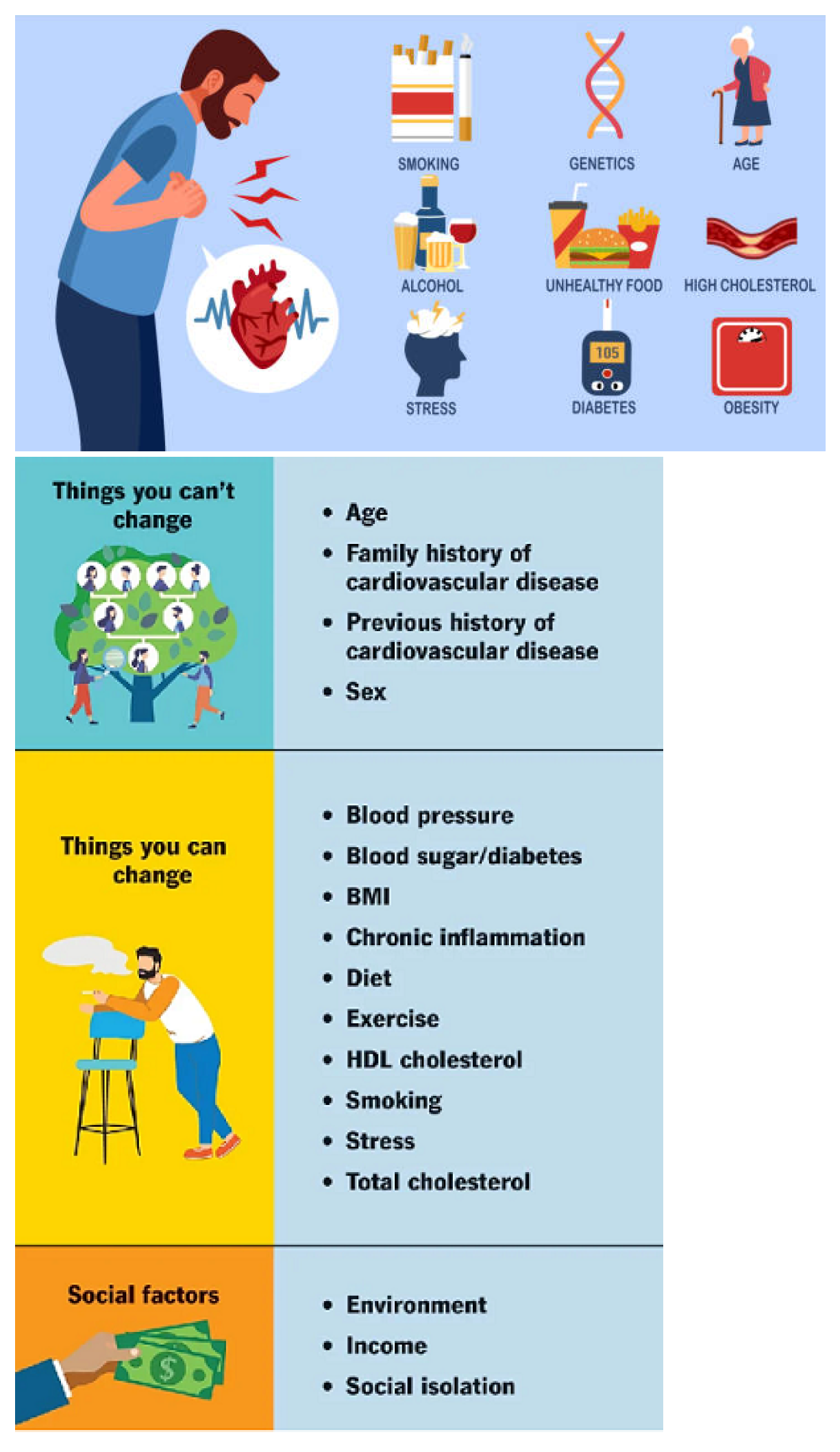
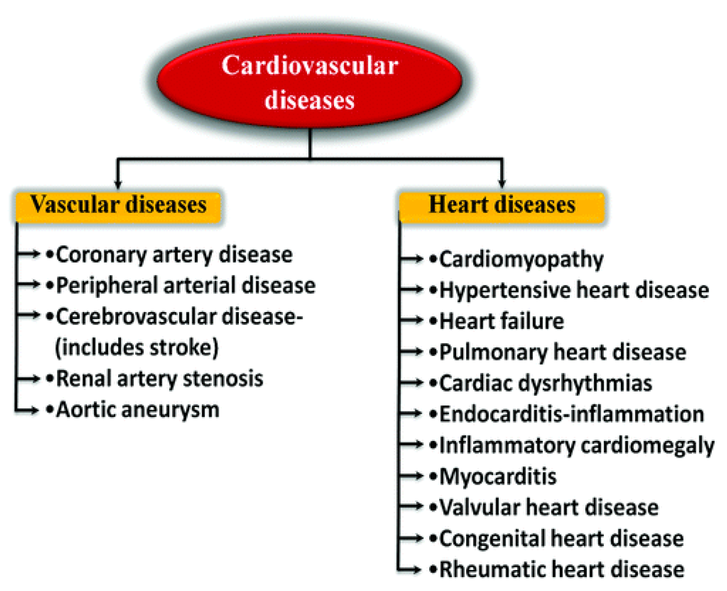
A PSV–NHFRS-based cardiac imaging modality, based on machine learning, has also been demonstrated, and a real-world application of the algorithm is given.

This article follows the format listed below. The core concepts underlying FS, NS, RS, SVNRS, and a few basic operational laws are examined in Section 2. In Section 3, we present novel aggregation operators, such as CL–PSV–NHFRWA and CL–PSV–NHFROWA. In Section 4, we present brand-new aggregation operators like CL–PSV–NHFRWG and CL–PSV–NHFROWG. A decision-making strategy based on the suggested AOs is constructed in Section 5 along with a solution to a numerical problem and numerical illustrations. In Section 6, we contrast some of the present practises with the recommended ones. In Section 7, we come to a conclusion.

2. Preliminaries

The fundamental concepts for NSs, SVNSs, SV–NRSs, scoring functions (SF), and accuracy functions (AF) are covered in this section.

Definition 1.

Addressing a certain set δ. A FS [12] Z in δ is presented as

$$Z=\left\{〈♭,{\mathsf{\Gamma }}_Z\left(♭\right)〉|♭\in \delta \right\},$$

for each $♭\in \delta ,$ the MD ${\mathsf{\Gamma }}_Z\left(♭\right):\delta \to \delta$ specifies the degree to which the element $♭\in Z,$ where ${\mathsf{\Gamma }}_Z\left(♭\right)\in \left[0,1\right].$

Definition 2.

Addressing a certain set δ. An IFS [5] A in δ is presented as

$$A=\left\{〈♭,\mathsf{\Gamma }\left(♭\right),\nabla \left(♭\right)〉|♭\in \delta \right\},$$

for each $♭\in \delta ,\mathsf{\Gamma }$ is the MD and ∇ is the NMD to the IFS $A,$ respectively, where $(\mathsf{\Gamma }\left(♭\right),\nabla \left(♭\right))\in \left[0,1\right]$ be the unit interval. Moreover, it is required that $0\le (\mathsf{\Gamma }\left(♭\right)+\nabla \left(♭\right))\le 1,$ for each $♭\in \delta$.

Definition 3.

Addressing a certain set δ and $\mathsf{{\rm Y}}\in \delta .$ A NS [28]♭ in δ is denoted as MD ${\mathsf{\Gamma }}_{♭}(\mathsf{{\rm Y}}),$ an IMD ${\nabla }_{♭}(\mathsf{{\rm Y}})$ and a NMD ${\Im }_{♭}(\mathsf{{\rm Y}})$. ${\mathsf{\Gamma }}_{♭}(\mathsf{{\rm Y}}),$${\nabla }_{♭}(\mathsf{{\rm Y}})$ and ${\Im }_{♭}(\mathsf{{\rm Y}})$ are real standard and non-standard subset of $\left]0^{-,}{1}^{+}\right[$ and

$${\mathsf{\Gamma }}_{♭}(\mathsf{{\rm Y}}),{\nabla }_{♭}(\mathsf{{\rm Y}}),{\Im }_{♭}(\mathsf{{\rm Y}}):\delta ⟶\left]0^{-,}{1}^{+}\right[$$

The representation of neutrosophic set (NS) ♭ is mathematically defined as:

$$♭=\left\{〈\mathsf{{\rm Y}},{\mathsf{\Gamma }}_{♭}(\mathsf{{\rm Y}}),{\nabla }_{♭}(\mathsf{{\rm Y}}),{\Im }_{♭}(\mathsf{{\rm Y}}))〉\right|\mathsf{{\rm Y}}\in \delta \},$$

where

$$0^{-}<{\mathsf{\Gamma }}_{♭}(\mathsf{{\rm Y}})+{\nabla }_{♭}(\mathsf{{\rm Y}})+{\Im }_{♭}(\mathsf{{\rm Y}})\le 3^{+}.$$

The real standard or non-standard $\left]0^{-},1^{+}\right[$ subsets are assumed to have value in the neutrosophic set from a logical perspective. For technological applications, one must, therefore, employ the interval $[0,1]$, rather than $\left]0^{-},1^{+}\right[$, because $\left]0^{-},1^{+}\right[$ is challenging to apply in operating systems, due to engineering and scientific difficulties. The idea of a single-valued neutrosipic set that lies in the range $[0,1]$ is then discussed.

Definition 4.

(See [49]). Addressing a certain set δ and $\mathsf{{\rm Y}}\in \delta .$ A SV-NS ♭ in δ is defined as MD ${\mathsf{\Gamma }}_{♭}(\mathsf{{\rm Y}}),$ an IMD ${\nabla }_{♭}(\mathsf{{\rm Y}})$ and a NMD ${\Im }_{♭}(\mathsf{{\rm Y}})$.

${\mathsf{\Gamma }}_{♭}(\mathsf{{\rm Y}}),$${\nabla }_{♭}(\mathsf{{\rm Y}})$ and ${\Im }_{♭}(\mathsf{{\rm Y}})$ are real standard and non-standard subset of $\left[0,1\right],$ and

$${\mathsf{\Gamma }}_{♭}(\mathsf{{\rm Y}}),{\nabla }_{♭}(\mathsf{{\rm Y}}),{\Im }_{♭}(\mathsf{{\rm Y}}):\delta ⟶\left[0,1\right].$$

The representation of SVNS ♭ is mathematically defined as:

$$♭=\left\{〈\mathsf{{\rm Y}},{\mathsf{\Gamma }}_{♭}(\mathsf{{\rm Y}}),{\nabla }_{♭}(\mathsf{{\rm Y}}),{\Im }_{♭}(\mathsf{{\rm Y}}))〉\right|\mathsf{{\rm Y}}\in \delta \},$$

where

$$0<{\mathsf{\Gamma }}_{♭}(\mathsf{{\rm Y}})+{\nabla }_{♭}(\mathsf{{\rm Y}})+{\Im }_{♭}(\mathsf{{\rm Y}})\le 3.$$

Definition 5.

([50]). Let F is a fixed set. The mathematically representation Probabilistic HF set (PHFS) Γ is defined as:

$$=\left\{\langle ♭,{\mathsf{\Gamma }}_{\top }(♭)/{\mathsf{\Lambda }}_{{}_{\top (♭)}}\rangle |♭\in F\right\}$$

where ${\mathsf{\Gamma }}_{\top }(♭)$ is a subset of $[0,1]$, and ${\mathsf{\Gamma }}_{\top }(♭)/{\mathsf{\Lambda }}_{♭}$ shows a MD of the element $♭\in F$ to the set Γ. And ${\mathsf{\Lambda }}_{♭}$ shows the possibilities with the property that ${\oplus }_{\mathsf{\ell }=1}^s{\mathsf{\Lambda }}_{{}_{{\top }_{\mathsf{\ell }}}}=1$.

Definition 6.

([51]). For a fixed set $Y,$ the $SV-NHFS$ F is mathematically represented as follows:

$$F=\left\{〈♭,{\mathsf{\Gamma }}_{{\top }_F}(♭),{\nabla }_{{\top }_F}(♭),{\Im }_{{\top }_F}(♭)〉\right|♭\in Y\},$$

where ${\mathsf{\Gamma }}_{{\top }_F}(♭),{\nabla }_{{\top }_F}(♭)$ and ${\Im }_{{\top }_F}(♭)$ are sets of some values in $\left[0,1\right]$, called the MD, IMD and NMD sequentially that must be satisfied the following properties:

$$\forall ♭\in Y,\forall {\mu }_F(♭)\in {\mathsf{\Gamma }}_{{\top }_F}(♭),\forall {\lambda }_F(♭)\in {\mathsf{\Gamma }}_{{\top }_F}(♭),$$

and

$$\forall {\nu }_F(♭)\in {\Im }_{{\top }_F}(♭)\mathrm{with}\left(max\left({\mathsf{\Gamma }}_{{\top }_F}(♭)\right)\right)+\left(min\left({\nabla }_{{\top }_F}(♭)\right)\right)+\left(min\left({\nabla }_{{\top }_F}(♭)\right)\right)\le 3,$$

and

$$\left(min\left({\mathsf{\Gamma }}_{{\top }_F}(♭)\right)\right)+\left(min\left({\nabla }_{{\top }_F}(♭)\right)\right)+\left(max\left({\Im }_{{\top }_F}(♭)\right)\right)\le 3.$$

For simplicity, we use a pair $F=$$({\mathsf{\Gamma }}_{{\top }_F},{\nabla }_{{\top }_F},{\Im }_{{\top }_F})$ to mean $SV-NHFS$.

Definition 7.

Let F be a fixed set, the mathematical representation of SV–neutrosophic PHFS (SV–NPHFS) [52], $\mathbb{N}$ is as,

$$\mathbb{N}=\left\{〈♭,{\mathsf{\Gamma }}_{{\top }_{\mathbb{N}}}(♭)/{\wp }_{{}_{\top (♭)}},{\nabla }_{{\top }_{\mathbb{N}}}(♭)/{\mathsf{\Lambda }}_{{}_{\top (♭)}},{\Im }_{{\top }_{\mathbb{N}}}(♭)/{\mathsf{\Xi }}_{{}_{\top (♭)}}〉\right|♭\in F\},$$

where

$$〈{\mathsf{\Gamma }}_{{\top }_{\mathbb{N}}}(♭)/{\wp }_{{}_{\top (♭)}},{\nabla }_{{\top }_{\mathbb{N}}}(♭)/{\mathsf{\Lambda }}_{{}_{\top (♭)}},{\Im }_{{\top }_{\mathbb{N}}}(♭)/{\mathsf{\Xi }}_{{}_{\top (♭)}}〉⟶[0,1],$$

and${\mathsf{\Gamma }}_{{\top }_{\mathbb{N}}}(♭)/{\wp }_{{}_{\top (♭)}},$${\nabla }_{{\top }_{\mathbb{N}}}(♭)/{\mathsf{\Lambda }}_{{}_{\top (♭)}},$${\Im }_{{\top }_{\mathbb{N}}}(♭)/{\mathsf{\Xi }}_{{}_{\top (♭)}}$ shows a MD, IMD and NMD respectively of the element $♭\in F$ to the set $\mathbb{N}$. And ${\wp }_{{}_{\top (♭)}},{\mathsf{\Lambda }}_{{}_{\top (♭)}},{\mathsf{\Xi }}_{{}_{\top (♭)}}$ shows the possibilities with the property that

$${\oplus }_{\mathsf{\ell }=1}^s{\wp }_{{}_{{\top }_{\mathsf{\ell }}}}=1,{\oplus }_{\mathsf{\ell }=1}^s{\mathsf{\Lambda }}_{{}_{{\top }_{\mathsf{\ell }}}}=1\mathrm{and}{\oplus }_{\mathsf{\ell }=1}^s{\mathsf{\Xi }}_{{}_{{\top }_{\mathsf{\ell }}}}=1.$$

Definition 8.

(See [53]). Assume η is a universal set and ℏ is relation on $\eta .$ A set valued mapping is defined as

$${\hslash }^{*}:\eta \to M\left(\eta \right)\mathrm{by}{\hslash }^{*}\left(\rho \right)=\{a\in \eta |(\rho ,a)\in \hslash \},$$

for $\rho \in \eta$ where ${\hslash }^{*}\left(\rho \right)$ is referred to as the element’s ρ successor neighborhood in connection to relation $\hslash .$ The pair $\left(\eta ,\hslash \right)$ is called (crisp) space of resemblance. Now for any set $\kappa \subseteq \eta ,$ the lower approximation (LA) and upper approximation (UA) of κ with respect to space of resemblance $\left(\eta ,\hslash \right)$ is defined as:

$$\begin{array}{ccc}\hfill \underline{\hslash }\left(\kappa \right)& =& \{\rho \in \eta |{\hslash }^{*}\left(\rho \right)\subseteq \kappa \};\hfill \\ \hfill \overline{\hslash }\left(\kappa \right)& =& \{\rho \in \eta |{\hslash }^{*}\left(\rho \right)\cap \kappa \ne \varphi \}.\hfill \end{array}$$

The pair $\left(\underline{\hslash }\left(\kappa \right),\overline{\hslash }\left(\kappa \right)\right)$ is called fuzzy RS where both $\underline{\hslash }\left(\kappa \right),\overline{\hslash }\left(\kappa \right):M\left(\eta \right)\to M\left(\eta \right)$ are upper and lower approximation operators.

Definition 9.

(See [54]). Assume universal set $\ddot{U}$ and let $\varrho \in SV-NHFRS(\ddot{U}\times \ddot{U})$ be $SV-NF$ relation. Then

(i) ϱ is reflexive if

$${\mathsf{\Gamma }}_{\varrho }(\wp ,\wp )=1,{\nabla }_{\varrho }(\wp ,\wp )=1\mathit{and}{\Im }_{\varrho }(\wp ,\wp )=1,\forall \wp \in \ddot{U};$$

(ii) ϱ is symmetric if

$$\begin{array}{ccc}\hfill \forall (\wp ,\mathsf{\Gamma })& \in & (\ddot{U}\times \ddot{U}),{\mathsf{\Gamma }}_{\varrho }(\wp ,\mathsf{\Gamma })={\mathsf{\Gamma }}_{\varrho }(\mathsf{\Gamma },\wp ),{\nabla }_{\varrho }(\wp ,\mathsf{\Gamma })={\nabla }_{\varrho }(\mathsf{\Gamma },\wp )\hfill \\ & & \mathit{and}\hfill \\ \hfill {\Im }_{\varrho }(\wp ,\mathsf{\Gamma })& =& {\Im }_{\varrho }(\mathsf{\Gamma },\wp );\hfill \end{array}$$

(iii) ϱ is transitive if $\forall (\wp ,t)\in (\ddot{U}\times \ddot{U}),$

$$\begin{array}{ccc}\hfill {\mathsf{\Gamma }}_{\varrho }(\mathsf{\Gamma },t)& \ge & {\vee }_{\wp \in \ddot{U}}[{\mathsf{\Gamma }}_{\varrho }(\mathsf{\Gamma },\wp )\wedge {\mathsf{\Gamma }}_{\varrho }(\wp ,t)],\hfill \\ \hfill {\nabla }_{\varrho }(\mathsf{\Gamma },t)& =& {\wedge }_{\wp \in \ddot{U}}[{\nabla }_{\varrho }(\mathsf{\Gamma },\wp )\vee {\nabla }_{\varrho }(\wp ,t)],\hfill \end{array}$$

and

$${\Im }_{\varrho }(\mathsf{\Gamma },t)={\wedge }_{\wp \in \ddot{U}}[{\Im }_{\varrho }(\mathsf{\Gamma },\wp )\vee {\Im }_{\varrho }(\wp ,t)].$$

Definition 10.

Assume universal set $\ddot{U}$ and let $\varrho \in SV-NHFRS(\ddot{U}\times \ddot{U})$ is a $SV-NF$ relation. the pair ($\ddot{U},\varrho$) represent a $SV-NF$ space of resemblance. Assume ℓ is any subset of $SV-NS\left(\ddot{U}\right)$ i.e $\mathsf{\ell }\subseteq SV-NS\left(\ddot{U}\right).$ Then on the bases of $SV-NF$ approximation space $(\ddot{U},\varrho ),$ then the lower and upper approximations of ℓ are represented as $\overline{\varrho }(\mathsf{\ell })$ and $\underline{\varrho }(\mathsf{\ell })$ given as following:

$$\overline{\varrho }(\mathsf{\ell })=\left\{〈\wp ,{\mathsf{\Gamma }}_{\overline{\varrho }(\mathsf{\ell })}(\wp ),{\nabla }_{\overline{\varrho }(\mathsf{\ell })}(\wp ),{\Im }_{\overline{\varrho }(\mathsf{\ell })}(\wp )〉\right|\wp \in \ddot{U}\},$$

$$\underline{\varrho }(\mathsf{\ell })=\left\{\langle \wp ,{\mathsf{\Gamma }}_{\underline{\varrho }(\mathsf{\ell })}(\wp ),{\nabla }_{\underline{\varrho }(\mathsf{\ell })}(\wp ),{\Im }_{\underline{\varrho }(\mathsf{\ell })}(\wp )\rangle \right|\wp \in \ddot{U}\},$$

where

$$\begin{array}{ccc}\hfill {\mathsf{\Gamma }}_{\overline{\varrho }(\mathsf{\ell })}(\wp )& =& {\vee }_{t\in \ddot{U}}[{\mathsf{\Gamma }}_{\varrho }(\wp ,t)\vee {\mathsf{\Gamma }}_{\varrho }\left(t\right)],\hfill \\ \hfill {\nabla }_{\overline{\varrho }(\mathsf{\ell })}(\wp )& =& {\wedge }_{t\in \ddot{U}}[{\nabla }_{\varrho }(\wp ,t)\wedge {\nabla }_{\varrho }\left(t\right)],\hfill \\ \hfill {\Im }_{\overline{\varrho }(\mathsf{\ell })}(\wp )& =& {\wedge }_{t\in \ddot{U}}[{\Im }_{\varrho }(\wp ,t)\wedge {\Im }_{\varrho }\left(t\right)],\hfill \\ \hfill {\mathsf{\Gamma }}_{\underline{\varrho }(\mathsf{\ell })}(\wp )& =& {\wedge }_{t\in \ddot{U}}[{\mathsf{\Gamma }}_{\varrho }(\wp ,t)\wedge {\mathsf{\Gamma }}_{\varrho }\left(t\right)],\hfill \\ \hfill {\nabla }_{\underline{\varrho }(\mathsf{\ell })}(\wp )& =& {\wedge }_{t\in \ddot{U}}[{\nabla }_{\varrho }(\wp ,t)\wedge {\nabla }_{\varrho }\left(t\right)],\hfill \\ \hfill {\Im }_{\underline{\varrho }(\mathsf{\ell })}(\wp )& =& {\vee }_{t\in \ddot{U}}[{\Im }_{\varrho }(\wp ,t)\vee {\Im }_{\varrho }\left(t\right)].\hfill \end{array}$$

such that

$$0<{\mathsf{\Gamma }}_{\overline{\varrho }(\mathsf{\ell })}(\wp )+{\nabla }_{\overline{\varrho }(\mathsf{\ell })}(\wp )+{\Im }_{\overline{\varrho }(\mathsf{\ell })}(\wp )\le 3,$$

and

$$0<{\mathsf{\Gamma }}_{\underline{\varrho }(\mathsf{\ell })}(\wp )+{\nabla }_{\underline{\varrho }(\mathsf{\ell })}(\wp )+{\Im }_{\underline{\varrho }(\mathsf{\ell })}(\wp )\le 3.$$

As $\underline{\varrho }(\mathsf{\ell })$ and $\overline{\varrho }(\mathsf{\ell })$ are $SV-NFSs,$ so $\overline{\varrho }(\mathsf{\ell }),\underline{\varrho }(\mathsf{\ell }):SV-NFS\left(\ddot{U}\right)⟶SV-NFS\left(\ddot{U}\right)$ are LA and UA operators. So the pair

$$\varrho (\mathsf{\ell })=(\underline{\varrho }(\mathsf{\ell }),\overline{\varrho }(\mathsf{\ell }))=\{\wp ,\langle ({\mathsf{\Gamma }}_{\underline{\varrho }(\mathsf{\ell })}(\wp ),{\nabla }_{\underline{\varrho }(\mathsf{\ell })}(\wp ),{\Im }_{\underline{\varrho }(\mathsf{\ell })}(\wp )),({\mathsf{\Gamma }}_{\overline{\varrho }(\mathsf{\ell })}(\wp ),{\nabla }_{\overline{\varrho }(\mathsf{\ell })}(\wp ),{\Im }_{\overline{\varrho }(\mathsf{\ell })}(\wp ))|\wp \in \ddot{U}\}$$

is called $SV-NF$ rough set. For simplicity it can be denoted as

$$\varrho (\mathsf{\ell })=(\underline{\varrho }(\mathsf{\ell }),\overline{\varrho }(\mathsf{\ell }))=(({\underline{\mathsf{\Gamma }}}_{{\top }_{\mathsf{\ell }}}/{\underline{\mathsf{\Xi }}}_{{\top }_{\mathsf{\ell }}},{\underline{\nabla }}_{{\top }_{\mathsf{\ell }}}/{\underline{\mathsf{\Lambda }}}_{{\top }_{\mathsf{\ell }}},{\underline{\Im }}_{{\top }_{\mathsf{\ell }}}/{\underline{\mho }}_{{\top }_{\mathsf{\ell }}}),({\overline{\mathsf{\Gamma }}}_{{\top }_{\mathsf{\ell }}}/{\overline{\mathsf{\Xi }}}_{{\top }_{\mathsf{\ell }}},{\overline{\nabla }}_{{\top }_{\mathsf{\ell }}}/{\overline{\mathsf{\Lambda }}}_{{\top }_{\mathsf{\ell }}},{\overline{\Im }}_{{\top }_{\mathsf{\ell }}}/{\overline{\mho }}_{{\top }_{\mathsf{\ell }}}))$$

are known as $SV-NF$ rough number ($SV-NFRN$).

Definition 11.

Let $F=\{({\underline{\mathsf{\Gamma }}}_{{\top }_{\mathsf{\ell }}}/{\underline{\mathsf{\Xi }}}_{{\top }_{\mathsf{\ell }}},{\underline{\nabla }}_{{\top }_{\mathsf{\ell }}}/{\underline{\mathsf{\Lambda }}}_{{\top }_{\mathsf{\ell }}},{\underline{\Im }}_{{\top }_{\mathsf{\ell }}}/{\underline{\mho }}_{{\top }_{\mathsf{\ell }}}),({\overline{\mathsf{\Gamma }}}_{{\top }_{\mathsf{\ell }}}/{\overline{\mathsf{\Xi }}}_{{\top }_{\mathsf{\ell }}},{\overline{\nabla }}_{{\top }_{\mathsf{\ell }}}/{\overline{\mathsf{\Lambda }}}_{{\top }_{\mathsf{\ell }}},{\overline{\Im }}_{{\top }_{\mathsf{\ell }}}/{\overline{\mho }}_{{\top }_{\mathsf{\ell }}})\}$ be a PSV-neutrosophic rough number (PSV-NHFRN). Then, SF and AF are describe as:

$$\begin{array}{ccc}\hfill Sc& =& \frac{1}{6}\left\{3+{\underline{\mathsf{\Gamma }}}_{{\top }_{\mathsf{\ell }}}/{\underline{\mathsf{\Xi }}}_{{\top }_{\mathsf{\ell }}}+{\overline{\mathsf{\Gamma }}}_{{\top }_{\mathsf{\ell }}}/{\overline{\mathsf{\Xi }}}_{{\top }_{\mathsf{\ell }}}-{\underline{\nabla }}_{{\top }_{\mathsf{\ell }}}/{\underline{\mathsf{\Lambda }}}_{{\top }_{\mathsf{\ell }}}-{\overline{\nabla }}_{{\top }_{\mathsf{\ell }}}/{\overline{\mathsf{\Lambda }}}_{{\top }_{\mathsf{\ell }}}-{\underline{\Im }}_{{\top }_{\mathsf{\ell }}}/{\underline{\mho }}_{{\top }_{\mathsf{\ell }}}-{\overline{\Im }}_{{\top }_{\mathsf{\ell }}}/{\overline{\mho }}_{{\top }_{\mathsf{\ell }}}\right\},S\in [0,1]\hfill \\ \hfill Ac& =& \frac{1}{6}\left\{3+{\underline{\mathsf{\Gamma }}}_{{\top }_{\mathsf{\ell }}}/{\underline{\mathsf{\Xi }}}_{{\top }_{\mathsf{\ell }}}+{\overline{\mathsf{\Gamma }}}_{{\top }_{\mathsf{\ell }}}/{\overline{\mathsf{\Xi }}}_{{\top }_{\mathsf{\ell }}}+{\underline{\nabla }}_{{\top }_{\mathsf{\ell }}}/{\underline{\mathsf{\Lambda }}}_{{\top }_{\mathsf{\ell }}}+{\overline{\nabla }}_{{\top }_{\mathsf{\ell }}}/{\overline{\mathsf{\Lambda }}}_{{\top }_{\mathsf{\ell }}}-{\underline{\Im }}_{{\top }_{\mathsf{\ell }}}/{\underline{\mho }}_{{\top }_{\mathsf{\ell }}}+{\overline{\Im }}_{{\top }_{\mathsf{\ell }}}/{\overline{\mho }}_{{\top }_{\mathsf{\ell }}}\right\},A\in [0,1].\hfill \end{array}$$

Definition 12.

For two PSV-NHFRNs

$$♭=\left\{\begin{array}{c}\left({\underline{\mathsf{\Gamma }}}_{{\top }_1}/{\underline{\mathsf{\Xi }}}_{{\top }_1},{\underline{\nabla }}_{{\top }_1}/{\underline{\mathsf{\Lambda }}}_{{\top }_1}/{\underline{\mathsf{\Lambda }}}_{{\top }_1},{\underline{\Im }}_{{\top }_1}/{\underline{\mho }}_{{\top }_1}\right),\\ \left({\overline{\mathsf{\Gamma }}}_{{\top }_1}/{\overline{\mathsf{\Xi }}}_{{\top }_1},{\overline{\nabla }}_{{\top }_1}/{\overline{\mathsf{\Lambda }}}_{{\top }_1},{\overline{\Im }}_{{\top }_1}/{\overline{\mho }}_{{\top }_1}\right)\end{array}\right\}$$

and

$$Y=\left\{\begin{array}{c}\left({\underline{\mathsf{\Gamma }}}_{{\top }_2}/{\underline{\mathsf{\Xi }}}_{{\top }_2},{\underline{\nabla }}_{{\top }_2}/{\underline{\mathsf{\Lambda }}}_{{\top }_2},{\underline{\Im }}_{{\top }_2}/{\underline{\mho }}_{{\top }_2}\right),\\ \left({\overline{\mathsf{\Gamma }}}_{{\top }_2}/{\overline{\mathsf{\Xi }}}_{{\top }_2},{\overline{\nabla }}_{{\top }_2}/{\overline{\mathsf{\Lambda }}}_{{\top }_2},{\overline{\Im }}_{{\top }_2}/{\overline{\mho }}_{{\top }_2}\right)\end{array}\right\},$$

The outcomes are as follows:

1

If $S(♭)>S\left(Y\right)$ then $♭>$$Y,$

2

If $S\left(A\right)<S\left(B\right)$ then $♭<Y,$

3

If $S\left(A\right)=S\left(B\right)$ then,

i

If $A(♭)>A\left(Y\right)$ then $♭>$$Y,$

ii

If $A(♭)<A\left(Y\right)$ then $♭<Y,$

iii

If $A(♭)=A\left(Y\right)$ then $♭=Y.$

3. CL–Probabilistic Single-Valued—Neutrosophic Hesitant Fuzzy Rough (CL–PSV-NHFR) Aggregation Operators

Here, we first talk about CI–PSV–NHFRWA AOs. We also go over the fundamental characteristics of the operators.

CL–PSV–NHFR Weighted Average (CI-PSV-NHFRWA) Aggregation Operators

We first discuss CL–PSVNHFR weighted average (CI–PSVNHFRWA) AO.

Definition 13.

Let ${\alpha }_{\mathsf{\ell }}=$$(\left({\underline{\mathsf{\Gamma }}}_{{\top }_{\mathsf{\ell }}}/{\underline{\mathsf{\Xi }}}_{{\top }_{\mathsf{\ell }}},{\underline{\nabla }}_{{\top }_{\mathsf{\ell }}}/{\underline{\mathsf{\Lambda }}}_{{\top }_{\mathsf{\ell }}},{\underline{\Im }}_{{\top }_{\mathsf{\ell }}}/{\underline{\mho }}_{{\top }_{\mathsf{\ell }}}\right),({\overline{\mathsf{\Gamma }}}_{{\top }_{\mathsf{\ell }}}/{\overline{\mathsf{\Xi }}}_{{\top }_{\mathsf{\ell }}},{\overline{\nabla }}_{{\top }_{\mathsf{\ell }}}/{\overline{\mathsf{\Lambda }}}_{{\top }_{\mathsf{\ell }}},$${\overline{\Im }}_{{\top }_{\mathsf{\ell }}}/{\overline{\mho }}_{{\top }_{\mathsf{\ell }}}\left)\right)$, $\mathsf{\ell }=1,2,\dots ,n$ be a collection of PSV–NHFRNs and ${\zeta }_{\mathsf{\ell }}$ be the CL of ${\alpha }_{\mathsf{\ell }}$ with $0\le {\zeta }_{\mathsf{\ell }}\le 1$.

Let $\delta$$={({\delta }_1,{\delta }_2,{\delta }_3\dots ,{\delta }_n)}^T$ be the weight vectors for PSV–NHFRNs with the condition ${\sum }_{\mathsf{\ell }=1}^n{\delta }_{\mathsf{\ell }}=1$. Then, the mapping $CL-PSV-NHFRWA:F^n\to F$ operator is given as $CL-PSV-NHFRWA$

$$\begin{array}{ccc}\hfill \left\{\begin{array}{c}({\alpha }_1,{\zeta }_1),({\alpha }_2,{\zeta }_2),\\ \dots ,({\alpha }_n,{\zeta }_n)\end{array}\right\}& =& {\oplus }_{\mathsf{\ell }=1}^n{\delta }_{\mathsf{\ell }}\left({\zeta }_{\mathsf{\ell }}{\alpha }_{\mathsf{\ell }}\right)\hfill \\ & =& \left\{\begin{array}{c}{\delta }_1\left({\zeta }_1{\alpha }_1\right)\oplus {\delta }_2\left({\zeta }_2{\alpha }_2\right)\oplus \\ {\delta }_3\left({\zeta }_3{\alpha }_3\right)\oplus \dots \oplus {\delta }_n\left({\zeta }_n{\alpha }_n\right)\end{array}\right\}.\hfill \end{array}$$

It is called the CL–PSV–NHFRWA operator.

Theorem 1.

Let ${\alpha }_{\mathsf{\ell }}=$ $\left(\left({\underline{\mathsf{\Gamma }}}_{{\top }_{\mathsf{\ell }}}/{\underline{\mathsf{\Xi }}}_{{\top }_{\mathsf{\ell }}},{\underline{\nabla }}_{{\top }_{\mathsf{\ell }}}/{\underline{\mathsf{\Lambda }}}_{{\top }_{\mathsf{\ell }}},{\underline{\Im }}_{{\top }_{\mathsf{\ell }}}/{\underline{\mho }}_{{\top }_{\mathsf{\ell }}}\right),\left({\overline{\mathsf{\Gamma }}}_{{\top }_{\mathsf{\ell }}}/{\overline{\mathsf{\Xi }}}_{{\top }_{\mathsf{\ell }}},{\overline{\nabla }}_{{\top }_{\mathsf{\ell }}}/{\overline{\mathsf{\Lambda }}}_{{\top }_{\mathsf{\ell }}},{\overline{\Im }}_{{\top }_{\mathsf{\ell }}}/{\overline{\mho }}_{{\top }_{\mathsf{\ell }}}\right)\right)$, $\mathsf{\ell }=1,2,\dots ,n$ be a collection of PSV–NHFRNs and ${\zeta }_{\mathsf{\ell }}$ be the CL of ${\alpha }_{\mathsf{\ell }}$ with $0\le {\zeta }_{\mathsf{\ell }}\le 1$.

Let $\delta$$={({\delta }_1,{\delta }_2,{\delta }_3\dots ,{\delta }_n)}^T$ be the weight vectors for PSV–NHFRNs with the condition ${\sum }_{\mathsf{\ell }}^n{\delta }_{\mathsf{\ell }}=1$ and ${\sum }_{\mathsf{\ell }}^n{\mathsf{\Xi }}_{\mathsf{\ell }}=1,{\sum }_{\mathsf{\ell }}^n{\mathsf{\Lambda }}_{\mathsf{\ell }}=1,{\sum }_{\mathsf{\ell }}^n{\mho }_{\mathsf{\ell }}=1$. Then $CL-PSV-NHFRWA$

$$\left\{\begin{array}{c}({\alpha }_1,{\zeta }_1),({\alpha }_2,{\zeta }_2),\\ \dots ,({\alpha }_n,{\zeta }_n)\end{array}\right\}=\left\{\begin{array}{c}\left\{\begin{array}{c}\left(1-\prod _{\mathsf{\ell }=1}^n{\left(1-{\underline{\mathsf{\Gamma }}}_{{\top }_{\mathsf{\ell }}}/{\underline{\mathsf{\Xi }}}_{{\top }_{\mathsf{\ell }}}\right)}^{{\zeta }_{\mathsf{\ell }}{\delta }_{\mathsf{\ell }}}\right),\\ \left(\prod _{\mathsf{\ell }=1}^n{\left({\underline{\nabla }}_{{\top }_{\mathsf{\ell }}}/{\underline{\mathsf{\Lambda }}}_{{\top }_{\mathsf{\ell }}}\right)}^{{\zeta }_{\mathsf{\ell }}{\delta }_{\mathsf{\ell }}}\right),\left(\prod _{\mathsf{\ell }=1}^n{\left({\underline{\Im }}_{{\top }_{\mathsf{\ell }}}/{\underline{\mho }}_{{\top }_{\mathsf{\ell }}}\right)}^{{\zeta }_{\mathsf{\ell }}{\delta }_{\mathsf{\ell }}}\right)\end{array}\right\}\\ \left\{\begin{array}{c}\left(1-\prod _{\mathsf{\ell }=1}^n{\left(1-{\overline{\mathsf{\Gamma }}}_{{\top }_{\mathsf{\ell }}}/{\overline{\mathsf{\Xi }}}_{{\top }_{\mathsf{\ell }}}\right)}^{{\zeta }_{\mathsf{\ell }}{\delta }_{\mathsf{\ell }}}\right),\\ \left(\prod _{\mathsf{\ell }=1}^n{\left({\overline{\nabla }}_{{\top }_{\mathsf{\ell }}}/{\overline{\mathsf{\Lambda }}}_{{\top }_{\mathsf{\ell }}}\right)}^{{}^{{\zeta }_{\mathsf{\ell }}{\delta }_{\mathsf{\ell }}}}\right),\left(\prod _{\mathsf{\ell }=1}^n{\left({\overline{\Im }}_{{\top }_{\mathsf{\ell }}}/{\overline{\mho }}_{{\top }_{\mathsf{\ell }}}\right)}^{{}^{{\zeta }_{\mathsf{\ell }}{\delta }_{\mathsf{\ell }}}}\right)\end{array}\right\}\end{array}\right\}$$

 Proof. 

For n = 2, we have

$$CL-PSV-NHFRWA\left(({\alpha }_1,{\zeta }_1),({\alpha }_2,{\zeta }_2)\right)={\delta }_1\left({\zeta }_1{\alpha }_1\right)\oplus {\delta }_2\left({\zeta }_2{\alpha }_2\right).$$

By using the operational laws for PSV-NHFRNs, we get

$$\begin{array}{ccc}\hfill {\zeta }_1{\alpha }_1& =& \left\{\begin{array}{c}\left(1-{\left(1-{\underline{\mathsf{\Gamma }}}_{{\top }_1}/{\underline{\mathsf{\Xi }}}_{{\top }_1}\right)}^{{\zeta }_1},{\underline{\nabla }}_{{\top }_1}/{\underline{\mathsf{\Lambda }}}_{{\top }_1}^{{\zeta }_1},{\underline{\Im }}_{{\top }_1}/{\underline{\mho }}_{{\top }_1}^{{\zeta }_1}\right),\\ 1-{\left(1-{\overline{\mathsf{\Gamma }}}_{{\top }_1}/{\overline{\mathsf{\Xi }}}_{{\top }_1}\right)}^{{\zeta }_1},{\overline{\nabla }}_{{\top }_1}/{\overline{\mathsf{\Lambda }}}_{{\top }_1}^{{\zeta }_1},{\overline{\Im }}_{{\top }_1}/{\overline{\mho }}_{{\top }_1}^{{\zeta }_1}\end{array}\right\}\hfill \\ & =& \left\{\begin{array}{c}\left({\underline{\mathsf{{\rm Y}}}}_1,{\underline{\mathsf{\Gamma }}}_1,{\underline{\mathsf{\Theta }}}_1\right),\\ \left({\overline{\mathsf{{\rm Y}}}}_1,{\overline{\mathsf{\Gamma }}}_1,{\overline{\mathsf{\Theta }}}_1\right)\end{array}\right\}.\hfill \end{array}$$

Then

$$\begin{array}{ccc}\hfill {\delta }_1\left({\zeta }_1{\alpha }_1\right)& =& \left\{\begin{array}{c}\left(1-{\left(1-{\underline{\mathsf{{\rm Y}}}}_1\right)}^{{\zeta }_1},{\underline{\mathsf{\Gamma }}}_1^{{\zeta }_1},{\underline{\mathsf{\Theta }}}_1^{{\zeta }_1}\right),\\ \left(1-{\left(1-{\overline{\mathsf{{\rm Y}}}}_1\right)}^{{\zeta }_1},{\overline{\mathsf{\Gamma }}}_1^{{\zeta }_1},{\overline{\mathsf{\Theta }}}_1^{{\zeta }_1}\right)\end{array}\right\}\hfill \\ & =& \left\{\begin{array}{c}\left\{\begin{array}{c}\left(1-{\left[1-\left\{1-{\left(1-{\underline{\mathsf{\Gamma }}}_{{\top }_1}/{\underline{\mathsf{\Xi }}}_{{\top }_1}\right)}^{{\zeta }_1}\right\}\right]}^{{\delta }_1}\right),\\ {\left({\underline{\nabla }}_{{\top }_1}/{\underline{\mathsf{\Lambda }}}_{{\top }_1}^{{\zeta }_1}\right)}^{{\delta }_1},{\left({\underline{\Im }}_{{\top }_1}/{\underline{\mho }}_{{\top }_1}^{{\zeta }_1}\right)}^{{\delta }_1}\end{array}\right\},\\ \left\{\begin{array}{c}\left(1-{\left[1-\left\{1-{\left(1-{\overline{\mathsf{\Gamma }}}_{{\top }_1}/{\overline{\mathsf{\Xi }}}_{{\top }_1}\right)}^{{\zeta }_1}\right\}\right]}^{{\delta }_1}\right),\\ {\left({\overline{\nabla }}_{{\top }_1}/{\overline{\mathsf{\Lambda }}}_{{\top }_1}^{{\zeta }_1}\right)}^{{\delta }_1},{\left({\overline{\Im }}_{{\top }_1}/{\overline{\mho }}_{{\top }_1}^{{\zeta }_1}\right)}^{{\delta }_1}\end{array}\right\}\end{array}\right\}\hfill \\ & =& \left\{\begin{array}{c}\left\{\begin{array}{c}\left(1-{\left(1-{\underline{\mathsf{\Gamma }}}_{{\top }_1}/{\underline{\mathsf{\Xi }}}_{{\top }_1}\right)}^{{\zeta }_1{\delta }_1}\right),\\ \left({\underline{\nabla }}_{{\top }_1}/{\underline{\mathsf{\Lambda }}}_{{\top }_1}^{{\delta }_1{\zeta }_1}\right),\left({\underline{\Im }}_{{\top }_1}/{\underline{\mho }}_{{\top }_1}^{{\delta }_1{\zeta }_1}\right)\end{array}\right\},\\ \left\{\begin{array}{c}\left(1-{\left(1-{\overline{\mathsf{\Gamma }}}_{{\top }_1}/{\overline{\mathsf{\Xi }}}_{{\top }_1}\right)}^{{\zeta }_1{\delta }_1}\right),\\ \left({\overline{\nabla }}_{{\top }_1}/{\overline{\mathsf{\Lambda }}}_{{\top }_1}^{{\delta }_1{\zeta }_1}\right),\left({\overline{\Im }}_{{\top }_1}/{\overline{\mho }}_{{\top }_1}^{{\delta }_1{\zeta }_1}\right)\end{array}\right\}\end{array}\right\}.\hfill \end{array}$$

Similarly, we can see that

$${\zeta }_2{\alpha }_2=\left\{\begin{array}{c}\left\{\begin{array}{c}\left(1-{\left(1-{\underline{\mathsf{\Gamma }}}_{{\top }_2}/{\underline{\mathsf{\Xi }}}_{{\top }_2}\right)}^{{\zeta }_2{\delta }_2}\right),\\ \left({\underline{\nabla }}_{{\top }_2}/{\underline{\mathsf{\Lambda }}}_{{\top }_2}^{{\delta }_2{\zeta }_2}\right),\left({\underline{\Im }}_{{\top }_2}/{\underline{\mho }}_{{\top }_2}^{{\delta }_2{\zeta }_2}\right)\end{array}\right\},\\ \left\{\begin{array}{c}\left(1-{\left(1-{\overline{\mathsf{\Gamma }}}_{{\top }_2}/{\overline{\mathsf{\Xi }}}_{{\top }_2}\right)}^{{\zeta }_2{\delta }_2}\right),\\ \left({\overline{\nabla }}_{{\top }_2}/{\overline{\mathsf{\Lambda }}}_{{\top }_2}^{{\delta }_2{\zeta }_2}\right),\left({\overline{\Im }}_{{\top }_2}/{\overline{\mho }}_{{\top }_2}^{{\delta }_2{\zeta }_2}\right)\end{array}\right\}\end{array}\right\}.$$

Then,

$$\begin{array}{ccc}\hfill CL-PSV-NHFRWA& =& \left(({\alpha }_1,{\zeta }_1),({\alpha }_2,{\zeta }_2)\right)={\delta }_1\left({\zeta }_1{\alpha }_1\right)\oplus {\delta }_2\left({\zeta }_2{\alpha }_2\right)\hfill \\ & =& \left\{\begin{array}{c}\left\{\begin{array}{c}\left\{\begin{array}{c}\left(1-{\left(1-{\underline{\mathsf{\Gamma }}}_{{\top }_1}/{\underline{\mathsf{\Xi }}}_{{\top }_1}\right)}^{{\zeta }_1{\delta }_1}\right)\\ +\left(1-{\left(1-{\underline{\mathsf{\Gamma }}}_{{\top }_2}/{\underline{\mathsf{\Xi }}}_{{\top }_2}\right)}^{{\zeta }_2{\delta }_2}\right)\\ -\left(1-{\left(1-{\underline{\mathsf{\Gamma }}}_{{\top }_1}/{\underline{\mathsf{\Xi }}}_{{\top }_1}\right)}^{{\zeta }_1{\delta }_1}\right)\\ -\left(1-{\left(1-{\underline{\mathsf{\Gamma }}}_{{\top }_2}/{\underline{\mathsf{\Xi }}}_{{\top }_2}\right)}^{{\zeta }_2{\delta }_2}\right)\end{array}\right\},\\ \left\{\left({\underline{\nabla }}_{{\top }_1}/{\underline{\mathsf{\Lambda }}}_{{\top }_1}^{{\delta }_1{\zeta }_1}\right)\left({\underline{\nabla }}_{{\top }_2}/{\underline{\mathsf{\Lambda }}}_{{\top }_2}^{{\delta }_2{\zeta }_2}\right)\right\},\\ \left\{\left({\underline{\Im }}_{{\top }_1}/{\underline{\mho }}_{{\top }_1}^{{\delta }_1{\zeta }_1}\right)\left({\underline{\Im }}_{{\top }_2}/{\underline{\mho }}_{{\top }_2}^{{\delta }_2{\zeta }_2}\right)\right\}\end{array}\right\},\\ \left\{\begin{array}{c}\left\{\begin{array}{c}\left(1-{\left(1-{\overline{\mathsf{\Gamma }}}_{{\top }_1}/{\overline{\mathsf{\Xi }}}_{{\top }_1}\right)}^{{\zeta }_1{\delta }_1}\right)\\ +\left(1-{\left(1-{\overline{\mathsf{\Gamma }}}_{{\top }_2}/{\overline{\mathsf{\Xi }}}_{{\top }_2}\right)}^{{\zeta }_2{\delta }_2}\right)\\ -\left(1-{\left(1-{\overline{\mathsf{\Gamma }}}_{{\top }_1}/{\overline{\mathsf{\Xi }}}_{{\top }_1}\right)}^{{\zeta }_1{\delta }_1}\right)\\ -\left(1-{\left(1-{\overline{\mathsf{\Gamma }}}_{{\top }_2}/{\overline{\mathsf{\Xi }}}_{{\top }_2}\right)}^{{\zeta }_2{\delta }_2}\right)\end{array}\right\},\\ \left\{\left({\overline{\nabla }}_{{\top }_1}/{\overline{\mathsf{\Lambda }}}_{{\top }_1}^{{\delta }_1{\zeta }_1}\right)\left({\overline{\nabla }}_{{\top }_2}/{\overline{\mathsf{\Lambda }}}_{{\top }_2}^{{\delta }_2{\zeta }_2}\right)\right\},\\ \left\{\left({\overline{\Im }}_{{\top }_1}/{\overline{\mho }}_{{\top }_1}^{{\delta }_1{\zeta }_1}\right)\left({\overline{\Im }}_{{\top }_2}/{\overline{\mho }}_{{\top }_2}^{{\delta }_2{\zeta }_2}\right)\right\}\end{array}\right\}\end{array}\right\}\hfill \end{array}$$

Thus,

$$\begin{array}{ccc}& & CL-PSV-NHFRWA\left\{({\alpha }_1,{\zeta }_1),({\alpha }_2,{\zeta }_2)\right\}\hfill \\ & =& \left(\begin{array}{c}\left\{\begin{array}{c}\left(1-\prod _{\mathsf{\ell }=1}^2{\left(1-{\underline{\mathsf{\Gamma }}}_{{\top }_{\mathsf{\ell }}}/{\underline{\mathsf{\Xi }}}_{{\top }_{\mathsf{\ell }}}\right)}^{{\zeta }_{\mathsf{\ell }}{\delta }_{\mathsf{\ell }}}\right),\\ \left(\prod _{\mathsf{\ell }=1}^2{\left({\underline{\nabla }}_{{\top }_{\mathsf{\ell }}}/{\underline{\mathsf{\Lambda }}}_{{\top }_{\mathsf{\ell }}}^{{\delta }_{\mathsf{\ell }}{\zeta }_{\mathsf{\ell }}}\right)}^{{}^{{\zeta }_{\mathsf{\ell }}{\delta }_{\mathsf{\ell }}}}\right),\\ \left(\prod _{\mathsf{\ell }=1}^2{\left({\underline{\Im }}_{{\top }_{\mathsf{\ell }}}/{\underline{\mho }}_{{\top }_{\mathsf{\ell }}}^{{\delta }_{\mathsf{\ell }}{\zeta }_{\mathsf{\ell }}}\right)}^{{}^{{\zeta }_{\mathsf{\ell }}{\delta }_{\mathsf{\ell }}}}\right)\end{array}\right\},\\ \left\{\begin{array}{c}\left(1-\prod _{\mathsf{\ell }=1}^2{\left(1-{\overline{\mathsf{\Gamma }}}_{{\top }_{\mathsf{\ell }}}/{\overline{\mathsf{\Xi }}}_{{\top }_{\mathsf{\ell }}}\right)}^{{\zeta }_{\mathsf{\ell }}{\delta }_{\mathsf{\ell }}}\right),\\ \left(\prod _{\mathsf{\ell }=1}^2{\left({\overline{\nabla }}_{{\top }_{\mathsf{\ell }}}/{\overline{\mathsf{\Lambda }}}_{{\top }_{\mathsf{\ell }}}\right)}^{{}^{{\zeta }_{\mathsf{\ell }}{\delta }_{\mathsf{\ell }}}}\right),\\ \left(\prod _{\mathsf{\ell }=1}^2{\left({\overline{\Im }}_{{\top }_{\mathsf{\ell }}}/{\overline{\mho }}_{{\top }_{\mathsf{\ell }}}\right)}^{{}^{{\zeta }_{\mathsf{\ell }}{\delta }_{\mathsf{\ell }}}}\right)\end{array}\right\}\end{array}\right)\hfill \end{array}$$

Suppose that the result is valid for $n=†,$ that is

$$\begin{array}{ccc}& & CL-PSV-NHFRWA\left\{({\alpha }_1,{\zeta }_1),({\alpha }_2,{\zeta }_2),\dots ,({\alpha }_{†},{\zeta }_{†})\right\}\hfill \\ & =& \left(\begin{array}{c}\left\{\begin{array}{c}\left(1-\prod _{\mathsf{\ell }=1}^{†}{\left(1-{\underline{\mathsf{\Gamma }}}_{{\top }_{\mathsf{\ell }}}/{\underline{\mathsf{\Xi }}}_{{\top }_{\mathsf{\ell }}}\right)}^{{\zeta }_{\mathsf{\ell }}{\delta }_{\mathsf{\ell }}}\right),\\ \left(\prod _{\mathsf{\ell }=1}^{†}{\left({\underline{\nabla }}_{{\top }_{\mathsf{\ell }}}/{\underline{\mathsf{\Lambda }}}_{{\top }_{\mathsf{\ell }}\mathsf{\ell }}^{{\delta }_{\mathsf{\ell }}{\zeta }_{\mathsf{\ell }}}\right)}^{{}^{{\zeta }_{\mathsf{\ell }}{\delta }_{\mathsf{\ell }}}}\right),\\ \left(\prod _{\mathsf{\ell }=1}^{†}{\left({\underline{\Im }}_{{\top }_{\mathsf{\ell }}}/{\underline{\mho }}_{{\top }_{\mathsf{\ell }}}^{{\delta }_{\mathsf{\ell }}{\zeta }_{\mathsf{\ell }}}\right)}^{{}^{{\zeta }_{\mathsf{\ell }}{\delta }_{\mathsf{\ell }}}}\right)\end{array}\right\},\\ \left\{\begin{array}{c}\left(1-\prod _{\mathsf{\ell }=1}^{†}{\left(1-{\overline{\mathsf{\Gamma }}}_{{\top }_{\mathsf{\ell }}}/{\overline{\mathsf{\Xi }}}_{{\top }_{\mathsf{\ell }}}\right)}^{{\zeta }_{\mathsf{\ell }}{\delta }_{\mathsf{\ell }}}\right),\\ \left(\prod _{\mathsf{\ell }=1}^{†}{\left({\overline{\nabla }}_{{\top }_{\mathsf{\ell }}}/{\overline{\mathsf{\Lambda }}}_{{\top }_{\mathsf{\ell }}}\right)}^{{}^{{\zeta }_{\mathsf{\ell }}{\delta }_{\mathsf{\ell }}}}\right),\\ \left(\prod _{\mathsf{\ell }=1}^{†}{\left({\overline{\Im }}_{{\top }_{\mathsf{\ell }}}/{\overline{\mho }}_{{\top }_{\mathsf{\ell }}}\right)}^{{}^{{\zeta }_{\mathsf{\ell }}{\delta }_{\mathsf{\ell }}}}\right)\end{array}\right\}\end{array}\right)\hfill \end{array}$$

Then, for $n=†+1,$ we get

$$\begin{array}{ccc}& & CL-PSV-NHFRWA\left\{({\alpha }_1,{\zeta }_1),({\alpha }_2,{\zeta }_2),\dots ,({\alpha }_{†},{\zeta }_{†}),({\alpha }_{†+1},{\zeta }_{†+1})\right\}\hfill \\ & =& \left\{\begin{array}{c}\left\{\left\{\begin{array}{c}\left(1-\prod _{\mathsf{\ell }=1}^{†}{\left(1-{\underline{\mathsf{\Gamma }}}_{{\top }_{\mathsf{\ell }}}/{\underline{\mathsf{\Xi }}}_{{\top }_{\mathsf{\ell }}}\right)}^{{\zeta }_{\mathsf{\ell }}{\delta }_{\mathsf{\ell }}}\right),\\ \left(\prod _{\mathsf{\ell }=1}^{†}{\left({\underline{\nabla }}_{{\top }_{\mathsf{\ell }}}/{\underline{\mathsf{\Lambda }}}_{{\top }_{\mathsf{\ell }}}\right)}^{{}^{{\zeta }_{\mathsf{\ell }}{\delta }_{\mathsf{\ell }}}}\right),\\ \left(\prod _{\mathsf{\ell }=1}^{†}{\left({\underline{\nabla }}_{{\top }_{\mathsf{\ell }}}/{\underline{\mathsf{\Lambda }}}_{{\top }_{\mathsf{\ell }}}\right)}^{{}^{{\zeta }_{\mathsf{\ell }}{\delta }_{\mathsf{\ell }}}}\right)\end{array}\right\},\left\{\begin{array}{c}\left(1-\prod _{\mathsf{\ell }=1}^{†}{\left(1-{\overline{\mathsf{\Gamma }}}_{{\top }_{\mathsf{\ell }}}/{\overline{\mathsf{\Xi }}}_{{\top }_{\mathsf{\ell }}}\right)}^{{\zeta }_{\mathsf{\ell }}{\delta }_{\mathsf{\ell }}}\right),\\ \left(\prod _{\mathsf{\ell }=1}^{†}{\left({\overline{\nabla }}_{{\top }_{\mathsf{\ell }}}/{\overline{\mathsf{\Lambda }}}_{{\top }_{\mathsf{\ell }}}\right)}^{{}^{{\zeta }_{\mathsf{\ell }}{\delta }_{\mathsf{\ell }}}}\right),\\ \left(\prod _{\mathsf{\ell }=1}^{†}{\left({\overline{\nabla }}_{{\top }_{\mathsf{\ell }}}/{\overline{\mathsf{\Lambda }}}_{{\top }_{\mathsf{\ell }}}\right)}^{{}^{{\zeta }_{\mathsf{\ell }}{\delta }_{\mathsf{\ell }}}}\right)\end{array}\right\}\right\}\oplus \\ \left\{\left\{\begin{array}{c}\left(1-{\left(1-{\underline{\mathsf{\Gamma }}}_{{\top }_{†+1}}/{\underline{\mathsf{\Xi }}}_{{\top }_{†+1}}\right)}^{{\zeta }_{†+1}{\delta }_{†+1}}\right),\\ {\left({\underline{\nabla }}_{{\top }_{†+1}}/{\underline{\mathsf{\Lambda }}}_{{\top }_{†+1}}\right)}^{{\delta }_{†+1}{\zeta }_{†+1}},\\ {\left({\underline{\Im }}_{{\top }_{\mathsf{\ell }}}/{\underline{\mho }}_{{\top }_{†+1}}\right)}^{{\delta }_{†+1}{\zeta }_{†+1}}\end{array}\right\},\left\{\begin{array}{c}\left(1-{\left(1-{\overline{\mathsf{\Gamma }}}_{{\top }_{†+1}}/{\overline{\mathsf{\Xi }}}_{{\top }_{†+1}}\right)}^{{\zeta }_{†+1}{\delta }_{†+1}}\right),\\ {\left({\overline{\nabla }}_{{\top }_{†+1}}/{\overline{\mathsf{\Lambda }}}_{{\top }_{†+1}}\right)}^{{\delta }_{†+1}{\zeta }_{†+1}},\\ {\left({\overline{\Im }}_{{\top }_{†+1}}/{\overline{\mho }}_{{\top }_{†+1}}\right)}^{{\delta }_{†+1}{\zeta }_{†+1}}\end{array}\right\}\right\}\end{array}\right\}\hfill \\ & =& \left\{\begin{array}{c}\left\{\begin{array}{c}\left\{\begin{array}{c}\left(1-\prod _{\mathsf{\ell }=1}^{†}{\left(1-{\underline{\mathsf{\Gamma }}}_{{\top }_{\mathsf{\ell }}}/{\underline{\mathsf{\Xi }}}_{{\top }_{\mathsf{\ell }}}\right)}^{{\zeta }_{\mathsf{\ell }}{\delta }_{\mathsf{\ell }}}\right)\\ +\left(1-{\left(1-{\underline{\mathsf{\Gamma }}}_{{\top }_{\mathsf{\ell }}}/{\underline{\mathsf{\Xi }}}_{{\top }_{\mathsf{\ell }}}\right)}^{{\zeta }_{†+1}{\delta }_{†+1}}\right)\\ -\left(1-\prod _{\mathsf{\ell }=1}^{†}{\left(1-{\underline{\mathsf{\Gamma }}}_{{\top }_{\mathsf{\ell }}}/{\underline{\mathsf{\Xi }}}_{{\top }_{\mathsf{\ell }}}\right)}^{{\zeta }_{\mathsf{\ell }}{\delta }_{\mathsf{\ell }}}\right)\\ \left(1-{\left(1-{\underline{\mathsf{\Gamma }}}_{{\top }_{\mathsf{\ell }}}/{\underline{\mathsf{\Xi }}}_{{\top }_{\mathsf{\ell }}}\right)}^{{\zeta }_{†+1}{\delta }_{†+1}}\right)\end{array}\right\},\\ \left\{\prod _{\mathsf{\ell }=1}^{†}{\left({\underline{\nabla }}_{{\top }_{\mathsf{\ell }}}/{\underline{\mathsf{\Lambda }}}_{{\top }_{\mathsf{\ell }}}\right)}^{{}^{{\zeta }_{\mathsf{\ell }}{\delta }_{\mathsf{\ell }}}},{\left({\underline{\nabla }}_{{\top }_{\mathsf{\ell }}}/{\underline{\mathsf{\Lambda }}}_{{\top }_{\mathsf{\ell }}†+1}\right)}^{{\delta }_{†+1}{\zeta }_{†+1}}\right\},\\ \left\{\prod _{\mathsf{\ell }=1}^{†}{\left({\underline{\Im }}_{{\top }_{\mathsf{\ell }}}/{\underline{\mho }}_{{\top }_{\mathsf{\ell }}}\right)}^{{}^{{\zeta }_{\mathsf{\ell }}{\delta }_{\mathsf{\ell }}}},{\left({\underline{\Im }}_{{\top }_{\mathsf{\ell }}}/{\underline{\mho }}_{{\top }_{\mathsf{\ell }}†+1}\right)}^{{\delta }_{†+1}{\zeta }_{†+1}}\right\}\end{array}\right\},\\ \left\{\begin{array}{c}\left\{\begin{array}{c}\left(1-\prod _{\mathsf{\ell }=1}^{†}{\left(1-{\overline{\mathsf{\Gamma }}}_{{\top }_{\mathsf{\ell }}}/{\overline{\mathsf{\Xi }}}_{{\top }_{\mathsf{\ell }}\mathsf{\ell }}\right)}^{{\zeta }_{\mathsf{\ell }}{\delta }_{\mathsf{\ell }}}\right)\\ +\left(1-{\left(1-{\overline{\mathsf{\Gamma }}}_{{\top }_{\mathsf{\ell }}}/{\overline{\mathsf{\Xi }}}_{{\top }_{\mathsf{\ell }}†+1}\right)}^{{\zeta }_{†+1}{\delta }_{†+1}}\right)\\ -\left(1-\prod _{\mathsf{\ell }=1}^{†}{\left(1-{\overline{\mathsf{\Gamma }}}_{{\top }_{\mathsf{\ell }}}/{\overline{\mathsf{\Xi }}}_{{\top }_{\mathsf{\ell }}\mathsf{\ell }}\right)}^{{\zeta }_{\mathsf{\ell }}{\delta }_{\mathsf{\ell }}}\right)\\ \left(1-{\left(1-{\overline{\mathsf{\Gamma }}}_{{\top }_{\mathsf{\ell }}}/{\overline{\mathsf{\Xi }}}_{{\top }_{\mathsf{\ell }}†+1}\right)}^{{\zeta }_{†+1}{\delta }_{†+1}}\right)\end{array}\right\},\\ \left\{\prod _{\mathsf{\ell }=1}^{†}{\left({\overline{\nabla }}_{{\top }_{\mathsf{\ell }}}/{\overline{\mathsf{\Lambda }}}_{{\top }_{\mathsf{\ell }}\mathsf{\ell }}\right)}^{{}^{{\zeta }_{\mathsf{\ell }}{\delta }_{\mathsf{\ell }}}},{\overline{\nabla }}_{{\top }_{\mathsf{\ell }}}/{\overline{\mathsf{\Lambda }}}_{{\top }_{\mathsf{\ell }}†+1}^{{\delta }_{†+1}{\zeta }_{†+1}}\right\},\\ \left\{\prod _{\mathsf{\ell }=1}^{†}{\left({\overline{\nabla }}_{{\top }_{\mathsf{\ell }}}/{\overline{\mathsf{\Lambda }}}_{{\top }_{\mathsf{\ell }}}\right)}^{{}^{{\zeta }_{\mathsf{\ell }}{\delta }_{\mathsf{\ell }}}},{\overline{\nabla }}_{{\top }_{\mathsf{\ell }}}/{\overline{\mathsf{\Lambda }}}_{{\top }_{†+1}}^{{\delta }_{†+1}{\zeta }_{†+1}}\right\}\end{array}\right\}\end{array}\right\}\hfill \\ & =& \left\{\begin{array}{c}\left\{\begin{array}{c}\left(1-\prod _{\mathsf{\ell }=1}^{†+1}{\left(1-{\underline{\mathsf{\Gamma }}}_{{\top }_{\mathsf{\ell }}}/{\underline{\mathsf{\Xi }}}_{{\top }_{\mathsf{\ell }}}\right)}^{{\zeta }_{\mathsf{\ell }}{\delta }_{\mathsf{\ell }}}\right),\\ \left(\prod _{\mathsf{\ell }=1}^{†+1}{\left({\underline{\nabla }}_{{\top }_{\mathsf{\ell }}}/{\underline{\mathsf{\Lambda }}}_{{\top }_{\mathsf{\ell }}}\right)}^{{}^{{\zeta }_{\mathsf{\ell }}{\delta }_{\mathsf{\ell }}}}\right),\\ \left(\prod _{\mathsf{\ell }=1}^{†+1}{\left({\underline{\Im }}_{{\top }_{\mathsf{\ell }}}/{\underline{\mho }}_{{\top }_{\mathsf{\ell }}\mathsf{\ell }}\right)}^{{}^{{\zeta }_{\mathsf{\ell }}{\delta }_{\mathsf{\ell }}}}\right)\end{array}\right\},\\ \left\{\begin{array}{c}\left\{1-\prod _{\mathsf{\ell }=1}^{†+1}{\left(1-{\overline{\mathsf{\Gamma }}}_{{\top }_{\mathsf{\ell }}}/{\overline{\mathsf{\Xi }}}_{{\top }_{\mathsf{\ell }}\mathsf{\ell }}\right)}^{{\zeta }_{\mathsf{\ell }}{\delta }_{\mathsf{\ell }}}\right\},\\ \left\{\prod _{\mathsf{\ell }=1}^{†+1}{\left({\overline{\nabla }}_{{\top }_{\mathsf{\ell }}}/{\overline{\mathsf{\Lambda }}}_{{\top }_{\mathsf{\ell }}\mathsf{\ell }}\right)}^{{}^{{\zeta }_{\mathsf{\ell }}{\delta }_{\mathsf{\ell }}}}\right\},\\ \left\{\prod _{\mathsf{\ell }=1}^{†+1}{\left({\overline{\Im }}_{{\top }_{\mathsf{\ell }}}/{\overline{\mho }}_{{\top }_{\mathsf{\ell }}\mathsf{\ell }}\right)}^{{}^{{\zeta }_{\mathsf{\ell }}{\delta }_{\mathsf{\ell }}}}\right\}\end{array}\right\}\end{array}\right\}\hfill \end{array}$$

Hence, the result is valid for $n=†+1$. Therefore, the result is valid for any number of PSV–NHFRNs. □

For the collection of PSV–NHFRNs ${\alpha }_{\mathsf{\ell }}=$$(\left({\underline{\mathsf{\Gamma }}}_{{\top }_{\mathsf{\ell }}}/{\underline{\mathsf{\Xi }}}_{{\top }_{\mathsf{\ell }}},{\underline{\nabla }}_{{\top }_{\mathsf{\ell }}}/{\underline{\mathsf{\Lambda }}}_{{\top }_{\mathsf{\ell }}},{\underline{\Im }}_{{\top }_{\mathsf{\ell }}}/{\underline{\mho }}_{{\top }_{\mathsf{\ell }}}\right),({\overline{\mathsf{\Gamma }}}_{{\top }_{\mathsf{\ell }}}/{\overline{\mathsf{\Xi }}}_{{\top }_{\mathsf{\ell }}},$${\overline{\nabla }}_{{\top }_{\mathsf{\ell }}}/{\overline{\mathsf{\Lambda }}}_{{\top }_{\mathsf{\ell }}},{\overline{\Im }}_{{\top }_{\mathsf{\ell }}}/{\overline{\mho }}_{{\top }_{\mathsf{\ell }}}\left)\right)$ where $\mathsf{\ell }=1,2,\dots ,n$ and ${\zeta }_{\mathsf{\ell }}$ is the CL of ${\alpha }_{\mathsf{\ell }}$ with $0\le {\zeta }_{\mathsf{\ell }}\le 1$ and $\mathsf{\Xi },\mathsf{\Lambda },\mho$ are the probabilities with condition ${\sum }_{\mathsf{\ell }}^n{\mathsf{\Xi }}_{\mathsf{\ell }}=1,{\sum }_{\mathsf{\ell }}^n{\mathsf{\Lambda }}_{\mathsf{\ell }}=1,{\sum }_{\mathsf{\ell }}^n{\mho }_{\mathsf{\ell }}=1$.

Let $\delta$$={({\delta }_1,{\delta }_2,{\delta }_3\dots ,{\delta }_n)}^T$ is the weight vectors for PSV–NHFRNs with the condition ${\sum }_{\mathsf{\ell }}^n{\delta }_{\mathsf{\ell }}=1$ and ${\sum }_{\mathsf{\ell }}^n{\mathsf{\Xi }}_{\mathsf{\ell }}=1,{\sum }_{\mathsf{\ell }}^n{\mathsf{\Lambda }}_{\mathsf{\ell }}=1,{\sum }_{\mathsf{\ell }}^n{\mho }_{\mathsf{\ell }}=1$.

Then CI–PSV–NHFRWA AOs have the following properties:

1. Idempotency

If for all $({\alpha }_{\mathsf{\ell }},{\zeta }_{\mathsf{\ell }})=(\alpha ,\zeta ),$ i.e., ${\mathsf{\Gamma }}_{\mathsf{\ell }}/{\mathsf{\Xi }}_{{\top }_{\mathsf{\ell }}}=\{{\underline{\mathsf{\Gamma }}}_{{\top }_{\mathsf{\ell }}}/{\underline{\mathsf{\Xi }}}_{{\top }_{\mathsf{\ell }}},{\overline{\mathsf{\Gamma }}}_{{\top }_{\mathsf{\ell }}}/{\overline{\mathsf{\Xi }}}_{{\top }_{\mathsf{\ell }}}\},$ ${\nabla }_{\mathsf{\ell }}/{\mathsf{\Lambda }}_{{\top }_{\mathsf{\ell }}}=\{{\underline{\nabla }}_{{\top }_{\mathsf{\ell }}}/{\underline{\mathsf{\Lambda }}}_{{\top }_{\mathsf{\ell }}},{\overline{\nabla }}_{{\top }_{\mathsf{\ell }}}/{\overline{\mathsf{\Lambda }}}_{{\top }_{\mathsf{\ell }}}\},$

${\Im }_{\mathsf{\ell }}/{\mho }_{{\top }_{\mathsf{\ell }}}=\{{\underline{\Im }}_{{\top }_{\mathsf{\ell }}}/{\underline{\mho }}_{{\top }_{\mathsf{\ell }}},{\overline{\Im }}_{{\top }_{\mathsf{\ell }}}/{\overline{\mho }}_{{\top }_{\mathsf{\ell }}}\},$${\zeta }_{\mathsf{\ell }}=\zeta ,$ then

$$CL-PSV-NHFRWA\left(({\alpha }_1,{\zeta }_1),({\alpha }_2,{\zeta }_2),\dots ,({\alpha }_n,{\zeta }_n)\right)={\zeta }_{\alpha }$$

 Proof. 

If $({\alpha }_{\mathsf{\ell }},{\zeta }_{\mathsf{\ell }})=(\alpha ,\zeta ),$ then by using Theorem 1, we get

$$\begin{array}{ccc}& & CL-PSV-NHFRWA\left\{({\alpha }_{{\top }_1},{\zeta }_1),({\alpha }_{{\top }_2},{\zeta }_2),\dots ,({\alpha }_{{\top }_n},{\zeta }_n)\right\}\hfill \\ & =& \left\{\begin{array}{c}\left\{\begin{array}{c}\left(1-\prod _{\mathsf{\ell }=1}^n{\left(1-{\underline{\mathsf{\Gamma }}}_{{\top }_{\mathsf{\ell }}}/{\underline{\mathsf{\Xi }}}_{{\top }_{\mathsf{\ell }}}\right)}^{\zeta {\delta }_{\mathsf{\ell }}}\right),\\ \left(\prod _{\mathsf{\ell }=1}^n{\left({\underline{\nabla }}_{{\top }_{\mathsf{\ell }}}/{\underline{\mathsf{\Lambda }}}_{{\top }_{\mathsf{\ell }}}\right)}^{{}^{{\zeta }_{\mathsf{\ell }}{\delta }_{\mathsf{\ell }}}}\right),\left(\prod _{\mathsf{\ell }=1}^n{\left({\underline{\Im }}_{{\top }_{\mathsf{\ell }}}/{\underline{\mho }}_{{\top }_{\mathsf{\ell }}}\right)}^{{}^{\zeta {\delta }_{\mathsf{\ell }}}}\right)\end{array}\right\},\\ \left\{\begin{array}{c}\left(1-\prod _{\mathsf{\ell }=1}^n{\left(1-{\overline{\mathsf{\Gamma }}}_{{\top }_{\mathsf{\ell }}}/{\overline{\mathsf{\Xi }}}_{{\top }_{\mathsf{\ell }}}\right)}^{\zeta {\delta }_{\mathsf{\ell }}}\right),\\ \left(\prod _{\mathsf{\ell }=1}^n{\left({\overline{\nabla }}_{{\top }_{\mathsf{\ell }}}/{\overline{\mathsf{\Lambda }}}_{{\top }_{\mathsf{\ell }}}\right)}^{\zeta {\delta }_{\mathsf{\ell }}}\right),\left(\prod _{\mathsf{\ell }=1}^n{\left({\overline{\Im }}_{{\top }_{\mathsf{\ell }}}/{\overline{\mho }}_{{\top }_{\mathsf{\ell }}}\right)}^{{}^{\zeta {\delta }_{\mathsf{\ell }}}}\right)\end{array}\right\}\end{array}\right\}\hfill \\ & =& \left\{\begin{array}{c}\left\{\begin{array}{c}\left(1-{\left(1-{\underline{\mathsf{\Gamma }}}_{{\top }_{\mathsf{\ell }}}/{\underline{\mathsf{\Xi }}}_{{\top }_{\mathsf{\ell }}}\right)}^{\zeta {\sum }_{\mathsf{\ell }=1}^n{\delta }_{\mathsf{\ell }}}\right),\\ \left({\left({\underline{\nabla }}_{{\top }_{\mathsf{\ell }}}/{\underline{\mathsf{\Lambda }}}_{{\top }_{\mathsf{\ell }}}\right)}^{\zeta {\sum }_{\mathsf{\ell }=1}^n{\delta }_{\mathsf{\ell }}}\right),\left({\left({\underline{\Im }}_{{\top }_{\mathsf{\ell }}}/{\underline{\mho }}_{{\top }_{\mathsf{\ell }}}\right)}^{\zeta {\sum }_{\mathsf{\ell }=1}^n{\delta }_{\mathsf{\ell }}}\right)\end{array}\right\},\\ \left\{\begin{array}{c}\left(1-{\left(1-{\overline{\mathsf{\Gamma }}}_{{\top }_{\mathsf{\ell }}}/{\overline{\mathsf{\Xi }}}_{{\top }_{\mathsf{\ell }}}\right)}^{\zeta {\sum }_{\mathsf{\ell }=1}^n{\delta }_{\mathsf{\ell }}}\right),\\ \left({\left({\overline{\nabla }}_{{\top }_{\mathsf{\ell }}}/{\overline{\mathsf{\Lambda }}}_{{\top }_{\mathsf{\ell }}}\right)}^{{}^{\zeta {\sum }_{\mathsf{\ell }=1}^n{\delta }_{\mathsf{\ell }}}}\right),\left({\left({\overline{\nabla }}_{{\top }_{\mathsf{\ell }}}/{\overline{\mathsf{\Lambda }}}_{{\top }_{\mathsf{\ell }}}\right)}^{{}^{\zeta {\sum }_{\mathsf{\ell }=1}^n{\delta }_{\mathsf{\ell }}}}\right)\end{array}\right\}\end{array}\right\}\hfill \\ & =& \left\{\begin{array}{c}\left\{\left(1-{\left(1-{\underline{\mathsf{\Gamma }}}_{{\top }_{\mathsf{\ell }}}/{\underline{\mathsf{\Xi }}}_{{\top }_{\mathsf{\ell }}}\right)}^{\zeta }\right),{\left({\underline{\nabla }}_{{\top }_{\mathsf{\ell }}}/{\underline{\mathsf{\Lambda }}}_{{\top }_{\mathsf{\ell }}}\right)}^{\zeta },{\left({\underline{\Im }}_{{\top }_{\mathsf{\ell }}}/{\underline{\mho }}_{{\top }_{\mathsf{\ell }}}\right)}^{\zeta }\right\},\\ \left\{\left(1-{\left(1-{\overline{\mathsf{\Gamma }}}_{{\top }_{\mathsf{\ell }}}/{\overline{\mathsf{\Xi }}}_{{\top }_{\mathsf{\ell }}}\right)}^{\zeta }\right),{\left({\overline{\nabla }}_{{\top }_{\mathsf{\ell }}}/{\overline{\mathsf{\Lambda }}}_{{\top }_{\mathsf{\ell }}}\right)}^{\zeta },{\left({\overline{\nabla }}_{{\top }_{\mathsf{\ell }}}/{\overline{\mathsf{\Lambda }}}_{{\top }_{\mathsf{\ell }}}\right)}^{\zeta }\right\}\end{array}\right\}={\zeta }_{\alpha }.\hfill \end{array}$$

2. Boundedness

Let

$${\alpha }_{\mathsf{\ell }}^{-}=\left\{\begin{array}{c}\left(min{\underline{\mathsf{\Gamma }}}_{{\top }_{\mathsf{\ell }}}/{\underline{\mathsf{\Xi }}}_{{\top }_{\mathsf{\ell }}},min{\underline{\nabla }}_{{\top }_{\mathsf{\ell }}}/{\underline{\mathsf{\Lambda }}}_{{\top }_{\mathsf{\ell }}},min{\underline{\Im }}_{{\top }_{\mathsf{\ell }}}/{\underline{\mho }}_{{\top }_{\mathsf{\ell }}}\right),\\ \left(max{\overline{\mathsf{\Gamma }}}_{{\top }_{\mathsf{\ell }}}/{\overline{\mathsf{\Xi }}}_{{\top }_{\mathsf{\ell }}},max{\overline{\nabla }}_{{\top }_{\mathsf{\ell }}}/{\overline{\mathsf{\Lambda }}}_{{\top }_{\mathsf{\ell }}},max{\overline{\nabla }}_{{\top }_{\mathsf{\ell }}}/{\overline{\mathsf{\Lambda }}}_{{\top }_{\mathsf{\ell }}}\right)\end{array}\right\},\mathrm{and}$$

$${\alpha }_{\mathsf{\ell }}^{+}=\left\{\begin{array}{c}\left(max{\underline{\mathsf{\Gamma }}}_{{\top }_{\mathsf{\ell }}}/{\underline{\mathsf{\Xi }}}_{{\top }_{\mathsf{\ell }}},max{\underline{\nabla }}_{{\top }_{\mathsf{\ell }}}/{\underline{\mathsf{\Lambda }}}_{{\top }_{\mathsf{\ell }}},max{\underline{\Im }}_{{\top }_{\mathsf{\ell }}}/{\underline{\mho }}_{{\top }_{\mathsf{\ell }}}\right),\\ \left(min{\overline{\mathsf{\Gamma }}}_{{\top }_{\mathsf{\ell }}}/{\overline{\mathsf{\Xi }}}_{{\top }_{\mathsf{\ell }}},min{\overline{\nabla }}_{{\top }_{\mathsf{\ell }}}/{\overline{\mathsf{\Lambda }}}_{{\top }_{\mathsf{\ell }}},min{\overline{\Im }}_{{\top }_{\mathsf{\ell }}}/{\overline{\mho }}_{{\top }_{\mathsf{\ell }}}\right)\end{array}\right\}.$$

□

Then, for all ${\delta }_{\mathsf{\ell }},$ we have

$${\alpha }_{\mathsf{\ell }}^{-}\le CL-PSV-NHFRWA\left\{\begin{array}{c}({\alpha }_1,{\zeta }_1),({\alpha }_2,{\zeta }_2),\\ \dots ,({\alpha }_n,{\zeta }_n)\end{array}\right\}\le {\alpha }_{\mathsf{\ell }}^{+}.$$

For every $\mathsf{\ell },$

$$\begin{array}{ccc}\hfill min({\underline{\mathsf{\Gamma }}}_{{\top }_{\mathsf{\ell }}}/{\underline{\mathsf{\Xi }}}_{{\top }_{\mathsf{\ell }}})& \le & {\underline{\mathsf{\Gamma }}}_{{\top }_{\mathsf{\ell }}}/{\underline{\mathsf{\Xi }}}_{{\top }_{\mathsf{\ell }}}\le max({\underline{\mathsf{\Gamma }}}_{{\top }_{\mathsf{\ell }}}/{\underline{\mathsf{\Xi }}}_{{\top }_{\mathsf{\ell }}})\hfill \\ & ⟹& 1-max({\underline{\mathsf{\Gamma }}}_{{\top }_{\mathsf{\ell }}}/{\underline{\mathsf{\Xi }}}_{{\top }_{\mathsf{\ell }}})\le 1-{\underline{\mathsf{\Gamma }}}_{{\top }_{\mathsf{\ell }}}/{\underline{\mathsf{\Xi }}}_{{\top }_{\mathsf{\ell }}}\le 1-min({\underline{\mathsf{\Gamma }}}_{{\top }_{\mathsf{\ell }}}/{\underline{\mathsf{\Xi }}}_{{\top }_{\mathsf{\ell }}})\hfill \end{array}$$

 Proof. 

Now for every $\delta ,$ we get

$$\begin{array}{ccc}& & \left\{\begin{array}{c}\left(\prod _{\mathsf{\ell }=1}^n{\left(1-max\left({\underline{\mathsf{\Gamma }}}_{{\top }_{\mathsf{\ell }}}/{\underline{\mathsf{\Xi }}}_{{\top }_{\mathsf{\ell }}}\right)\right)}^{\left(max{\zeta }_{\mathsf{\ell }}\right){\delta }_{\mathsf{\ell }}}\right)\\ \le \left(\prod _{\mathsf{\ell }=1}^n{\left(1-{\underline{\mathsf{\Gamma }}}_{{\top }_{\mathsf{\ell }}}/{\underline{\mathsf{\Xi }}}_{{\top }_{\mathsf{\ell }}}\right)}^{{\zeta }_{\mathsf{\ell }}{\delta }_{\mathsf{\ell }}}\right)\\ \le \left(\prod _{\mathsf{\ell }=1}^n{\left(1-min\left({\underline{\mathsf{\Gamma }}}_{{\top }_{\mathsf{\ell }}}/{\underline{\mathsf{\Xi }}}_{{\top }_{\mathsf{\ell }}}\right)\right)}^{\left(min{\zeta }_{\mathsf{\ell }}\right){\delta }_{\mathsf{\ell }}}\right)\end{array}\right\}\hfill \\ & ⟹& \left\{\begin{array}{c}\left({\left(1-max\left({\underline{\mathsf{\Gamma }}}_{{\top }_{\mathsf{\ell }}}/{\underline{\mathsf{\Xi }}}_{{\top }_{\mathsf{\ell }}}\right)\right)}^{\left(max{\zeta }_{\mathsf{\ell }}\right){\sum }_{\mathsf{\ell }=1}^n{\delta }_{\mathsf{\ell }}}\right)\\ \le \left(\prod _{\mathsf{\ell }=1}^n{\left(1-{\underline{\mathsf{\Gamma }}}_{{\top }_{\mathsf{\ell }}}/{\underline{\mathsf{\Xi }}}_{{\top }_{\mathsf{\ell }}}\right)}^{{\zeta }_{\mathsf{\ell }}{\delta }_{\mathsf{\ell }}}\right)\\ \le \left({\left(1-min\left({\underline{\mathsf{\Gamma }}}_{{\top }_{\mathsf{\ell }}}/{\underline{\mathsf{\Xi }}}_{{\top }_{\mathsf{\ell }}}\right)\right)}^{\left(min{\zeta }_{\mathsf{\ell }}\right){\sum }_{\mathsf{\ell }=1}^n{\delta }_{\mathsf{\ell }}}\right)\end{array}\right\}\hfill \\ & ⟹& \left\{\begin{array}{c}\left(1-{\left(1-min\left({\underline{\mathsf{\Gamma }}}_{{\top }_{\mathsf{\ell }}}/{\underline{\mathsf{\Xi }}}_{{\top }_{\mathsf{\ell }}}\right)\right)}^{\left(min{\zeta }_{\mathsf{\ell }}\right)}\right)\\ \le \left(1-\prod _{\mathsf{\ell }=1}^n{\left(1-{\underline{\mathsf{\Gamma }}}_{{\top }_{\mathsf{\ell }}}/{\underline{\mathsf{\Xi }}}_{{\top }_{\mathsf{\ell }}}\right)}^{{\zeta }_{\mathsf{\ell }}{\delta }_{\mathsf{\ell }}}\right)\\ \le \left(1-{\left(1-max\left({\underline{\mathsf{\Gamma }}}_{{\top }_{\mathsf{\ell }}}/{\underline{\mathsf{\Xi }}}_{{\top }_{\mathsf{\ell }}}\right)\right)}^{\left(max{\zeta }_{\mathsf{\ell }}\right){\delta }_{\mathsf{\ell }}}{\underline{\mathsf{\Gamma }}}_{{\top }_{\mathsf{\ell }}}/{\underline{\mathsf{\Xi }}}_{{\top }_{\mathsf{\ell }}}\right)\\ \le \left(1-\prod _{\mathsf{\ell }=1}^n{\left(1-{\underline{\mathsf{\Gamma }}}_{{\top }_{\mathsf{\ell }}}/{\underline{\mathsf{\Xi }}}_{{\top }_{\mathsf{\ell }}}\right)}^{{\zeta }_{\mathsf{\ell }}{\delta }_{\mathsf{\ell }}}\right)\le \left({\underline{\mathsf{\Gamma }}}_{{\top }_{\mathsf{\ell }}}/{\underline{\mathsf{\Xi }}}_{{\top }_{\mathsf{\ell }}}\right)\end{array}\right\}.\hfill \end{array}$$

□

Similarly, for every ℓ,

$$\begin{array}{ccc}\hfill min({\overline{\mathsf{\Gamma }}}_{{\top }_{\mathsf{\ell }}}/{\overline{\mathsf{\Xi }}}_{{\top }_{\mathsf{\ell }}\mathsf{\ell }})& \le & {\overline{\mathsf{\Gamma }}}_{{\top }_{\mathsf{\ell }}}/{\overline{\mathsf{\Xi }}}_{{\top }_{\mathsf{\ell }}\mathsf{\ell }}\le max({\overline{\mathsf{\Gamma }}}_{{\top }_{\mathsf{\ell }}}/{\overline{\mathsf{\Xi }}}_{{\top }_{\mathsf{\ell }}\mathsf{\ell }})\hfill \\ & ⟹& 1-max({\overline{\mathsf{\Gamma }}}_{{\top }_{\mathsf{\ell }}}/{\overline{\mathsf{\Xi }}}_{{\top }_{\mathsf{\ell }}\mathsf{\ell }})\le 1-{\overline{\mathsf{\Gamma }}}_{{\top }_{\mathsf{\ell }}}/{\overline{\mathsf{\Xi }}}_{{\top }_{\mathsf{\ell }}\mathsf{\ell }}\le 1-min({\overline{\mathsf{\Gamma }}}_{{\top }_{\mathsf{\ell }}}/{\overline{\mathsf{\Xi }}}_{{\top }_{\mathsf{\ell }}\mathsf{\ell }}).\hfill \end{array}$$

Now for every $\delta ,$ we obtain

$$\begin{array}{ccc}& & \left\{\begin{array}{c}\left(\prod _{\mathsf{\ell }=1}^n{\left(1-max\left({\overline{\mathsf{\Gamma }}}_{{\top }_{\mathsf{\ell }}}/{\overline{\mathsf{\Xi }}}_{{\top }_{\mathsf{\ell }}}\right)\right)}^{\left(max{\zeta }_{\mathsf{\ell }}\right){\delta }_{\mathsf{\ell }}}\right)\\ \le \left(\prod _{\mathsf{\ell }=1}^n{\left(1-{\overline{\mathsf{\Gamma }}}_{{\top }_{\mathsf{\ell }}}/{\overline{\mathsf{\Xi }}}_{{\top }_{\mathsf{\ell }}}\right)}^{{\zeta }_{\mathsf{\ell }}{\delta }_{\mathsf{\ell }}}\right)\\ \le \left(\prod _{\mathsf{\ell }=1}^n{\left(1-min\left({\overline{\mathsf{\Gamma }}}_{{\top }_{\mathsf{\ell }}}/{\overline{\mathsf{\Xi }}}_{{\top }_{\mathsf{\ell }}}\right)\right)}^{\left(min{\zeta }_{\mathsf{\ell }}\right){\delta }_{\mathsf{\ell }}}\right)\end{array}\right\}\hfill \\ & ⟹& \left\{\begin{array}{c}\left({\left(1-max\left({\overline{\mathsf{\Gamma }}}_{{\top }_{\mathsf{\ell }}}/{\overline{\mathsf{\Xi }}}_{{\top }_{\mathsf{\ell }}}\right)\right)}^{\left(max{\zeta }_{\mathsf{\ell }}\right){\sum }_{\mathsf{\ell }=1}^n{\delta }_{\mathsf{\ell }}}\right)\\ \le \left(\prod _{\mathsf{\ell }=1}^n{\left(1-{\mathsf{\Gamma }}_{\mathsf{\ell }}\right)}^{{\zeta }_{\mathsf{\ell }}{\delta }_{\mathsf{\ell }}}\right)\\ \le \left({\left(1-min\left({\overline{\mathsf{\Gamma }}}_{{\top }_{\mathsf{\ell }}}/{\overline{\mathsf{\Xi }}}_{{\top }_{\mathsf{\ell }}}\right)\right)}^{\left(min{\zeta }_{\mathsf{\ell }}\right){\sum }_{\mathsf{\ell }=1}^n{\delta }_{\mathsf{\ell }}}\right)\end{array}\right\}\hfill \\ & ⟹& \left\{\begin{array}{c}\left(1-{\left(1-min\left({\mathsf{\Gamma }}_{\mathsf{\ell }}\right)\right)}^{\left(min{\zeta }_{\mathsf{\ell }}\right)}\right)\\ \le \left(1-\prod _{\mathsf{\ell }=1}^n{\left(1-{\mathsf{\Gamma }}_{\mathsf{\ell }}\right)}^{{\zeta }_{\mathsf{\ell }}{\delta }_{\mathsf{\ell }}}\right)\\ \le \left(1-{\left(1-max\left({\mathsf{\Gamma }}_{\mathsf{\ell }}\right)\right)}^{\left(max{\zeta }_{\mathsf{\ell }}\right){\delta }_{\mathsf{\ell }}}{\mathsf{\Gamma }}_{{\alpha }_{\mathsf{\ell }}{\zeta }_{\mathsf{\ell }}}^{min}\right)\\ \le \left(1-\prod _{\mathsf{\ell }=1}^n{\left(1-{\mathsf{\Gamma }}_{\mathsf{\ell }}\right)}^{{\zeta }_{\mathsf{\ell }}{\delta }_{\mathsf{\ell }}}\right)\le {\mathsf{\Gamma }}_{{\alpha }_{\mathsf{\ell }}{\zeta }_{\mathsf{\ell }}}^{max}.\end{array}\right\}.\hfill \end{array}$$

Similarly,

$$\begin{array}{ccc}& & \left\{\begin{array}{c}\left(min({\underline{\nabla }}_{{\top }_{\mathsf{\ell }}}/{\underline{\mathsf{\Lambda }}}_{{\top }_{\mathsf{\ell }}})\le {\underline{\nabla }}_{{\top }_{\mathsf{\ell }}}/{\underline{\mathsf{\Lambda }}}_{{\top }_{\mathsf{\ell }}}\le max({\underline{\nabla }}_{{\top }_{\mathsf{\ell }}}/{\underline{\mathsf{\Lambda }}}_{{\top }_{\mathsf{\ell }}})\right)\\ \iff min{({\underline{\nabla }}_{{\top }_{\mathsf{\ell }}}/{\underline{\mathsf{\Lambda }}}_{{\top }_{\mathsf{\ell }}})}^{min{\zeta }_{\mathsf{\ell }}}\le \prod _{\mathsf{\ell }=1}^n{\left({\underline{\nabla }}_{{\top }_{\mathsf{\ell }}}/{\underline{\mathsf{\Lambda }}}_{{\top }_{\mathsf{\ell }}}\right)}^{{\zeta }_{\mathsf{\ell }}{\delta }_{\mathsf{\ell }}}\\ \le max{({\underline{\nabla }}_{{\top }_{\mathsf{\ell }}}/{\underline{\mathsf{\Lambda }}}_{{\top }_{\mathsf{\ell }}})}^{max{\zeta }_{\mathsf{\ell }}}\end{array}\right\}\hfill \\ & ⟹& \left\{{\left({\underline{\nabla }}_{{\top }_{\mathsf{\ell }}}/{\underline{\mathsf{\Lambda }}}_{{\top }_{\mathsf{\ell }}}^{min}\right)}^{{\alpha }_{\mathsf{\ell }}{\zeta }_{\mathsf{\ell }}}\le \prod _{\mathsf{\ell }=1}^n{\left({\underline{\nabla }}_{{\top }_{\mathsf{\ell }}}/{\underline{\mathsf{\Lambda }}}_{{\top }_{\mathsf{\ell }}}\right)}^{{\zeta }_{\mathsf{\ell }}{\delta }_{\mathsf{\ell }}}\le {\left({\underline{\nabla }}_{{\top }_{\mathsf{\ell }}}/{\underline{\mathsf{\Lambda }}}_{{\top }_{\mathsf{\ell }}}^{max}\right)}^{{\alpha }_{\mathsf{\ell }}{\zeta }_{\mathsf{\ell }}}\right\}\hfill \end{array}$$

and

$$\begin{array}{ccc}& & \left\{\begin{array}{c}\left(min\left({\overline{\nabla }}_{{\top }_{\mathsf{\ell }}}/{\overline{\mathsf{\Lambda }}}_{{\top }_{\mathsf{\ell }}}\right)\le {\overline{\nabla }}_{{\top }_{\mathsf{\ell }}}/{\overline{\mathsf{\Lambda }}}_{{\top }_{\mathsf{\ell }}}\le max\left({\overline{\nabla }}_{{\top }_{\mathsf{\ell }}}/{\overline{\mathsf{\Lambda }}}_{{\top }_{\mathsf{\ell }}}\right)\right)\\ \iff min{({\overline{\nabla }}_{{\top }_{\mathsf{\ell }}}/{\overline{\mathsf{\Lambda }}}_{{\top }_{\mathsf{\ell }}})}^{min{\zeta }_{\mathsf{\ell }}}\le \prod _{\mathsf{\ell }=1}^n{\left({\overline{\nabla }}_{{\top }_{\mathsf{\ell }}}/{\overline{\mathsf{\Lambda }}}_{{\top }_{\mathsf{\ell }}}\right)}^{{\zeta }_{\mathsf{\ell }}{\delta }_{\mathsf{\ell }}}\\ \le max{({\overline{\nabla }}_{{\top }_{\mathsf{\ell }}}/{\overline{\mathsf{\Lambda }}}_{{\top }_{\mathsf{\ell }}})}^{max{\zeta }_{\mathsf{\ell }}}\end{array}\right\}\hfill \\ & ⟹& \left\{{\left({\overline{\nabla }}_{{\top }_{\mathsf{\ell }}}/{\overline{\mathsf{\Lambda }}}_{{\top }_{\mathsf{\ell }}}^{min}\right)}^{{\alpha }_{\mathsf{\ell }}{\zeta }_{\mathsf{\ell }}}\le \prod _{\mathsf{\ell }=1}^n{\left({\overline{\nabla }}_{{\top }_{\mathsf{\ell }}}/{\overline{\mathsf{\Lambda }}}_{{\top }_{\mathsf{\ell }}\mathsf{\ell }}\right)}^{{\zeta }_{\mathsf{\ell }}{\delta }_{\mathsf{\ell }}}\le {\left({\overline{\nabla }}_{{\top }_{\mathsf{\ell }}}/{\overline{\mathsf{\Lambda }}}_{{\top }_{\mathsf{\ell }}}^{max}\right)}^{{\alpha }_{\mathsf{\ell }}{\zeta }_{\mathsf{\ell }}}\right\}.\hfill \end{array}$$

Also,

$$\begin{array}{ccc}& & \left\{\begin{array}{c}min({\underline{\Im }}_{{\top }_{\mathsf{\ell }}}/{\underline{\mho }}_{{\top }_{\mathsf{\ell }}})\le {\underline{\Im }}_{{\top }_{\mathsf{\ell }}}/{\underline{\mho }}_{{\top }_{\mathsf{\ell }}}\le max({\underline{\Im }}_{{\top }_{\mathsf{\ell }}}/{\underline{\mho }}_{{\top }_{\mathsf{\ell }}})\\ \iff min{({\underline{\Im }}_{{\top }_{\mathsf{\ell }}}/{\underline{\mho }}_{{\top }_{\mathsf{\ell }}})}^{min{\zeta }_{\mathsf{\ell }}}\le \prod _{\mathsf{\ell }=1}^n{\left({\underline{\Im }}_{{\top }_{\mathsf{\ell }}}/{\underline{\mho }}_{{\top }_{\mathsf{\ell }}}\right)}^{{\zeta }_{\mathsf{\ell }}{\delta }_{\mathsf{\ell }}}\\ \le max{({\underline{\Im }}_{{\top }_{\mathsf{\ell }}}/{\underline{\mho }}_{{\top }_{\mathsf{\ell }}})}^{max{\zeta }_{\mathsf{\ell }}}\end{array}\right\}\hfill \\ & ⟹& \left\{{\left({\underline{\Im }}_{{\top }_{\mathsf{\ell }}}/{\underline{\mho }}_{{\top }_{\mathsf{\ell }}}^{min}\right)}^{{\alpha }_{\mathsf{\ell }}{\zeta }_{\mathsf{\ell }}}\le \prod _{\mathsf{\ell }=1}^n{\left({\underline{\Im }}_{{\top }_{\mathsf{\ell }}}/{\underline{\mho }}_{{\top }_{\mathsf{\ell }}}\right)}^{{\zeta }_{\mathsf{\ell }}{\delta }_{\mathsf{\ell }}}\le {\left({\underline{\Im }}_{{\top }_{\mathsf{\ell }}}/{\underline{\mho }}_{{\top }_{\mathsf{\ell }}}^{max}\right)}^{{\alpha }_{\mathsf{\ell }}{\zeta }_{\mathsf{\ell }}}\right\}\hfill \end{array}$$

and

$$\begin{array}{ccc}& & \left\{\begin{array}{c}min\left({\overline{\Im }}_{{\top }_{\mathsf{\ell }}}/{\overline{\mho }}_{{\top }_{\mathsf{\ell }}}\right)\le {\overline{\Im }}_{{\top }_{\mathsf{\ell }}}/{\overline{\mho }}_{{\top }_{\mathsf{\ell }}}\le max\left({\overline{\Im }}_{{\top }_{\mathsf{\ell }}}/{\overline{\mho }}_{{\top }_{\mathsf{\ell }}}\right)\\ \iff min{({\overline{\Im }}_{{\top }_{\mathsf{\ell }}}/{\overline{\mho }}_{{\top }_{\mathsf{\ell }}})}^{min{\zeta }_{\mathsf{\ell }}}\le \prod _{\mathsf{\ell }=1}^n{\left({\overline{\Im }}_{{\top }_{\mathsf{\ell }}}/{\overline{\mho }}_{{\top }_{\mathsf{\ell }}}\right)}^{{\zeta }_{\mathsf{\ell }}{\delta }_{\mathsf{\ell }}}\\ \le max{({\overline{\Im }}_{{\top }_{\mathsf{\ell }}}/{\overline{\mho }}_{{\top }_{\mathsf{\ell }}})}^{max{\zeta }_{\mathsf{\ell }}}\end{array}\right\}\hfill \\ & ⟹& \left\{{\left({\overline{\Im }}_{{\top }_{\mathsf{\ell }}}/{\overline{\mho }}_{{\top }_{\mathsf{\ell }}}^{min}\right)}^{{\alpha }_{\mathsf{\ell }}{\zeta }_{\mathsf{\ell }}}\le \prod _{\mathsf{\ell }=1}^n{\left({\overline{\Im }}_{{\top }_{\mathsf{\ell }}}/{\overline{\mho }}_{{\top }_{\mathsf{\ell }}}\right)}^{{\zeta }_{\mathsf{\ell }}{\delta }_{\mathsf{\ell }}}\le {\left({\overline{\Im }}_{{\top }_{\mathsf{\ell }}}/{\overline{\mho }}_{{\top }_{\mathsf{\ell }}}^{max}\right)}^{{\alpha }_{\mathsf{\ell }}{\zeta }_{\mathsf{\ell }}}\right\}.\hfill \end{array}$$

If

$$\begin{array}{ccc}\hfill CL-SV-NRWA\left\{\begin{array}{c}({\alpha }_1,{\zeta }_1),({\alpha }_2,{\zeta }_2),\\ \dots ,({\alpha }_n,{\zeta }_n)\end{array}\right\}& =& \alpha \hfill \\ & =& \left\{\begin{array}{c}\left({\underline{\mathsf{\Gamma }}}_{{\top }_{\mathsf{\ell }}}/{\underline{\mathsf{\Xi }}}_{{\top }_{\mathsf{\ell }}},{\underline{\nabla }}_{{\top }_{\mathsf{\ell }}}/{\underline{\mathsf{\Lambda }}}_{{\top }_{\mathsf{\ell }}},{\underline{\Im }}_{{\top }_{\mathsf{\ell }}}/{\underline{\mho }}_{{\top }_{\mathsf{\ell }}}\right),\\ \left({\overline{\mathsf{\Gamma }}}_{{\top }_{\mathsf{\ell }}}/{\overline{\mathsf{\Xi }}}_{{\top }_{\mathsf{\ell }}},{\overline{\nabla }}_{{\top }_{\mathsf{\ell }}}/{\overline{\mathsf{\Lambda }}}_{{\top }_{\mathsf{\ell }}},{\overline{\Im }}_{{\top }_{\mathsf{\ell }}}/{\overline{\mho }}_{{\top }_{\mathsf{\ell }}}\right)\end{array}\right\},\hfill \end{array}$$

then from the above analysis, we obtain

$$\left\{\begin{array}{c}\left\{\begin{array}{c}\left({\underline{\mathsf{\Gamma }}}_{{\top }_{\mathsf{\ell }}}/{\underline{\mathsf{\Xi }}}_{{\top }_{\mathsf{\ell }}}\le {\underline{\mathsf{\Gamma }}}_{{\top }_{\mathsf{\ell }}}/{\underline{\mathsf{\Xi }}}_{{\top }_{\mathsf{\ell }}}\le {\underline{\mathsf{\Gamma }}}_{{\top }_{\mathsf{\ell }}}/{\underline{\mathsf{\Xi }}}_{{\top }_{\mathsf{\ell }}}\right),\\ \left({\left({\overline{\mathsf{\Gamma }}}_{{\top }_{\mathsf{\ell }}}/{\overline{\mathsf{\Xi }}}_{{\top }_{\mathsf{\ell }}}^{min}\right)}^{{\alpha }_{\mathsf{\ell }}{\zeta }_{\mathsf{\ell }}}\le {\left({\overline{\mathsf{\Gamma }}}_{{\top }_{\mathsf{\ell }}}/{\overline{\mathsf{\Xi }}}_{{\top }_{\mathsf{\ell }}}\right)}^{{\alpha }_{\mathsf{\ell }}{\zeta }_{\mathsf{\ell }}}\le {\left({\overline{\mathsf{\Gamma }}}_{{\top }_{\mathsf{\ell }}}/{\overline{\mathsf{\Xi }}}_{{\top }_{\mathsf{\ell }}}^{max}\right)}^{{\alpha }_{\mathsf{\ell }}{\zeta }_{\mathsf{\ell }}}\right)\end{array}\right\},\\ \left\{\begin{array}{c}\left({\left({\underline{\nabla }}_{{\top }_{\mathsf{\ell }}}/{\underline{\mathsf{\Lambda }}}_{{\top }_{\mathsf{\ell }}}^{min}\right)}^{{\alpha }_{\mathsf{\ell }}{\zeta }_{\mathsf{\ell }}}\le {\left({\underline{\nabla }}_{{\top }_{\mathsf{\ell }}}/{\underline{\mathsf{\Lambda }}}_{{\top }_{\mathsf{\ell }}}\right)}^{{\alpha }_{\mathsf{\ell }}{\zeta }_{\mathsf{\ell }}}\le {\left({\underline{\nabla }}_{{\top }_{\mathsf{\ell }}}/{\underline{\mathsf{\Lambda }}}_{{\top }_{\mathsf{\ell }}}^{max}\right)}^{{\alpha }_{\mathsf{\ell }}{\zeta }_{\mathsf{\ell }}}\right),\\ \left({\left({\overline{\nabla }}_{{\top }_{\mathsf{\ell }}}/{\overline{\mathsf{\Lambda }}}_{{\top }_{\mathsf{\ell }}}^{min}\right)}^{{\alpha }_{\mathsf{\ell }}{\zeta }_{\mathsf{\ell }}}\le {\left({\overline{\nabla }}_{{\top }_{\mathsf{\ell }}}/{\overline{\mathsf{\Lambda }}}_{{\top }_{\mathsf{\ell }}}\right)}^{{\alpha }_{\mathsf{\ell }}{\zeta }_{\mathsf{\ell }}}\le {\left({\overline{\nabla }}_{{\top }_{\mathsf{\ell }}}/{\overline{\mathsf{\Lambda }}}_{{\top }_{\mathsf{\ell }}}^{max}\right)}^{{\alpha }_{\mathsf{\ell }}{\zeta }_{\mathsf{\ell }}}\right)\end{array}\right\},\\ \left\{\begin{array}{c}\left({\left({\underline{\Im }}_{{\top }_{\mathsf{\ell }}}/{\underline{\mho }}_{{\top }_{\mathsf{\ell }}}^{min}\right)}^{{\alpha }_{\mathsf{\ell }}{\zeta }_{\mathsf{\ell }}}\le {\left({\underline{\Im }}_{{\top }_{\mathsf{\ell }}}/{\underline{\mho }}_{{\top }_{\mathsf{\ell }}}\right)}^{{\alpha }_{\mathsf{\ell }}{\zeta }_{\mathsf{\ell }}}\le {\left({\underline{\Im }}_{{\top }_{\mathsf{\ell }}}/{\underline{\mho }}_{{\top }_{\mathsf{\ell }}}^{max}\right)}^{{\alpha }_{\mathsf{\ell }}{\zeta }_{\mathsf{\ell }}}\right),\\ \left({\left({\overline{\Im }}_{{\top }_{\mathsf{\ell }}}/{\overline{\mho }}_{{\top }_{\mathsf{\ell }}}^{min}\right)}^{{\alpha }_{\mathsf{\ell }}{\zeta }_{\mathsf{\ell }}}\le {\left({\overline{\Im }}_{{\top }_{\mathsf{\ell }}}/{\overline{\mho }}_{{\top }_{\mathsf{\ell }}}\right)}^{{\alpha }_{\mathsf{\ell }}{\zeta }_{\mathsf{\ell }}}\le {\left({\overline{\Im }}_{{\top }_{\mathsf{\ell }}}/{\overline{\mho }}_{{\top }_{\mathsf{\ell }}}^{max}\right)}^{{\alpha }_{\mathsf{\ell }}{\zeta }_{\mathsf{\ell }}}\right)\end{array}\right\}\end{array}\right\}.$$

Then, by using the definition of SF, we can conclude that

$${\alpha }_{\mathsf{\ell }}^{-}\le CL-PSV-NHFRWA\left\{\begin{array}{c}({\alpha }_1,{\zeta }_1),({\alpha }_2,{\zeta }_2),\\ \dots ,({\alpha }_n,{\zeta }_n)\end{array}\right\}\le {\alpha }_{\mathsf{\ell }}^{+}$$

3. Monotonicity

Let

$${\alpha }_{\mathsf{\ell }}^{*}=\left\{\begin{array}{c}\left({\underline{\mathsf{\Gamma }}}_{{\top }_{\mathsf{\ell }}}/{\underline{\mathsf{\Xi }}}_{{\top }_{\mathsf{\ell }}},{\underline{\nabla }}_{{\top }_{\mathsf{\ell }}}/{\underline{\mathsf{\Lambda }}}_{{\top }_{\mathsf{\ell }}{\alpha }_{\mathsf{\ell }}^{*}},{\underline{\Im }}_{{\top }_{\mathsf{\ell }}}/{\underline{\mho }}_{{\top }_{\mathsf{\ell }}{\alpha }_{\mathsf{\ell }}^{*}}\right),\\ \left({\overline{\mathsf{\Gamma }}}_{{\top }_{\mathsf{\ell }}}/{\overline{\mathsf{\Xi }}}_{{\top }_{\mathsf{\ell }}{\alpha }_{\mathsf{\ell }}^{*}},{\overline{\nabla }}_{{\top }_{\mathsf{\ell }}}/{\overline{\mathsf{\Lambda }}}_{{\top }_{\mathsf{\ell }}{\alpha }_{\mathsf{\ell }}^{*}},{\overline{\Im }}_{{\top }_{\mathsf{\ell }}}/{\overline{\mho }}_{{\top }_{\mathsf{\ell }}{\alpha }_{\mathsf{\ell }}^{*}}\right)\end{array}\right\}\left(\mathsf{\ell }=1,2,3,\cdots ,n\right)$$

be another collection of PSV–NHFRNs such that

$$\left\{\begin{array}{c}\left\{\begin{array}{c}\left({\underline{\mathsf{\Gamma }}}_{{\top }_{\mathsf{\ell }}}/{\underline{\mathsf{\Xi }}}_{{\top }_{\mathsf{\ell }}}\le {\underline{\mathsf{\Gamma }}}_{{\top }_{\mathsf{\ell }}}/{\underline{\mathsf{\Xi }}}_{{\top }_{\mathsf{\ell }}}\right),\\ \left(\left({\underline{\nabla }}_{{\top }_{\mathsf{\ell }}}/{\underline{\mathsf{\Lambda }}}_{{\top }_{\mathsf{\ell }{\alpha }_{\mathsf{\ell }}}}\right)\ge \left({\underline{\nabla }}_{{\top }_{\mathsf{\ell }}}/{\underline{\mathsf{\Lambda }}}_{{\top }_{\mathsf{\ell }}{\alpha }_{\mathsf{\ell }}^{*}}\right)\right),\\ \left(\left({\underline{\Im }}_{{\top }_{\mathsf{\ell }}}/{\underline{\mho }}_{{\top }_{\mathsf{\ell }}{\alpha }_{\mathsf{\ell }}}\right)\ge \left({\underline{\Im }}_{{\top }_{\mathsf{\ell }}}/{\underline{\mho }}_{{\top }_{\mathsf{\ell }}{\alpha }_{\mathsf{\ell }}^{*}}\right)\right)\end{array}\right\},\\ \left\{\begin{array}{c}\left(\left({\overline{\mathsf{\Gamma }}}_{{\top }_{\mathsf{\ell }}}/{\overline{\mathsf{\Xi }}}_{{\top }_{\mathsf{\ell }}{\alpha }_{\mathsf{\ell }}}\right)\le \left({\overline{\mathsf{\Gamma }}}_{{\top }_{\mathsf{\ell }}}/{\overline{\mathsf{\Xi }}}_{{\top }_{\mathsf{\ell }}{\alpha }_{\mathsf{\ell }}^{*}}\right)\right),\\ \left(\left({\overline{\nabla }}_{{\top }_{\mathsf{\ell }}}/{\overline{\mathsf{\Lambda }}}_{{\top }_{\mathsf{\ell }}{\alpha }_{\mathsf{\ell }}}\right)\ge \left({\overline{\nabla }}_{{\top }_{\mathsf{\ell }}}/{\overline{\mathsf{\Lambda }}}_{{\top }_{\mathsf{\ell }}{\alpha }_{\mathsf{\ell }}^{*}}\right)\right),\\ \left(\left({\overline{\Im }}_{{\top }_{\mathsf{\ell }}}/{\overline{\mho }}_{{\top }_{\mathsf{\ell }}{\alpha }_{\mathsf{\ell }}}\right)\ge \left({\overline{\Im }}_{{\top }_{\mathsf{\ell }}}/{\overline{\mho }}_{{\top }_{\mathsf{\ell }}{\alpha }_{\mathsf{\ell }}^{*}}\right)\right)\end{array}\right\}\end{array}\right\}$$

for all ${\delta }_{\mathsf{\ell }}.$ Then

$$\begin{array}{ccc}& & CL-PSV-NHFRWA\left\{\begin{array}{c}({\alpha }_1,{\zeta }_1),({\alpha }_2,{\zeta }_2),\\ \dots ,({\alpha }_n,{\zeta }_n)\end{array}\right\}\hfill \\ & \le & CL-PSV-NHFRWA\left\{\begin{array}{c}({\alpha }_1^{*},{\zeta }_1),({\alpha }_2^{*},{\zeta }_2),\\ \dots ,({\alpha }_n^{*},{\zeta }_n)\end{array}\right\}.\hfill \end{array}$$

 Proof. 

Since

$$\left\{\begin{array}{c}\left\{\begin{array}{c}\left(\left({\underline{\mathsf{\Gamma }}}_{{\top }_{\mathsf{\ell }}}/{\underline{\mathsf{\Xi }}}_{{\top }_{\mathsf{\ell }}{\alpha }_{\mathsf{\ell }}}\right)\le \left({\underline{\mathsf{\Gamma }}}_{{\top }_{\mathsf{\ell }}}/{\underline{\mathsf{\Xi }}}_{{\top }_{\mathsf{\ell }}{\alpha }_{\mathsf{\ell }}^{*}}\right)\right),\\ \left(\left({\underline{\nabla }}_{{\top }_{\mathsf{\ell }}}/{\underline{\mathsf{\Lambda }}}_{{\top }_{\mathsf{\ell }}{\alpha }_{\mathsf{\ell }}}\right)\ge \left({\underline{\nabla }}_{{\top }_{\mathsf{\ell }}}/{\underline{\mathsf{\Lambda }}}_{{\top }_{\mathsf{\ell }}{\alpha }_{\mathsf{\ell }}^{*}}\right)\right),\\ \left(\left({\underline{\Im }}_{{\top }_{\mathsf{\ell }}}/{\underline{\mho }}_{{\top }_{\mathsf{\ell }}{\alpha }_{\mathsf{\ell }}}\right)\ge \left({\underline{\Im }}_{{\top }_{\mathsf{\ell }}}/{\underline{\mho }}_{{\top }_{\mathsf{\ell }}{\alpha }_{\mathsf{\ell }}^{*}}\right)\right)\end{array}\right\},\\ \left\{\begin{array}{c}\left(\left({\overline{\mathsf{\Gamma }}}_{{\top }_{\mathsf{\ell }}}/{\overline{\mathsf{\Xi }}}_{{\top }_{\mathsf{\ell }}{\alpha }_{\mathsf{\ell }}}\right)\le \left({\overline{\mathsf{\Gamma }}}_{{\top }_{\mathsf{\ell }}}/{\overline{\mathsf{\Xi }}}_{{\top }_{\mathsf{\ell }}{\alpha }_{\mathsf{\ell }}^{*}}\right)\right),\\ \left(\left({\overline{\nabla }}_{{\top }_{\mathsf{\ell }}}/{\overline{\mathsf{\Lambda }}}_{{\top }_{\mathsf{\ell }}{\alpha }_{\mathsf{\ell }}}\right)\ge \left({\overline{\nabla }}_{{\top }_{\mathsf{\ell }}}/{\overline{\mathsf{\Lambda }}}_{{\top }_{\mathsf{\ell }}{\alpha }_{\mathsf{\ell }}^{*}}\right)\right),\\ \left(\left({\overline{\Im }}_{{\top }_{\mathsf{\ell }}}/{\overline{\mho }}_{{\top }_{\mathsf{\ell }}{\alpha }_{\mathsf{\ell }}}\right)\ge \left({\overline{\Im }}_{{\top }_{\mathsf{\ell }}}/{\overline{\mho }}_{{\top }_{\mathsf{\ell }}{\alpha }_{\mathsf{\ell }}^{*}}\right)\right)\end{array}\right\}\end{array}\right\}$$

for all $\mathsf{\ell },$

$$\left\{\begin{array}{c}\left\{\left(1-{\underline{\mathsf{\Gamma }}}_{{\top }_{\mathsf{\ell }}}/{\underline{\mathsf{\Xi }}}_{{\top }_{\mathsf{\ell }}}\le 1-{\underline{\mathsf{\Gamma }}}_{{\top }_{\mathsf{\ell }}}/{\underline{\mathsf{\Xi }}}_{{\top }_{\mathsf{\ell }}}\right)\right\}\\ ⟹\left\{\begin{array}{c}\left(\prod _{\mathsf{\ell }=1}^n{\left(1-{\underline{\mathsf{\Gamma }}}_{{\top }_{\mathsf{\ell }}}/{\underline{\mathsf{\Xi }}}_{{\top }_{\mathsf{\ell }}}\right)}^{{\zeta }_{\mathsf{\ell }}{\delta }_{\mathsf{\ell }}}\right)\\ \le \left(\prod _{\mathsf{\ell }=1}^n{\left(1-{\underline{\mathsf{\Gamma }}}_{{\top }_{\mathsf{\ell }}}/{\underline{\mathsf{\Xi }}}_{{\top }_{\mathsf{\ell }}}\right)}^{{\zeta }_{\mathsf{\ell }}{\delta }_{\mathsf{\ell }}}\right)\end{array}\right\}\\ ⟹\left\{\begin{array}{c}\left(1-\prod _{\mathsf{\ell }=1}^n{\left(1-{\underline{\mathsf{\Gamma }}}_{{\top }_{\mathsf{\ell }}}/{\underline{\mathsf{\Xi }}}_{{\top }_{\mathsf{\ell }}}\right)}^{{\zeta }_{\mathsf{\ell }}{\delta }_{\mathsf{\ell }}}\right)\\ \le \left(1-\prod _{\mathsf{\ell }=1}^n{\left(1-{\underline{\mathsf{\Gamma }}}_{{\top }_{\mathsf{\ell }}}/{\underline{\mathsf{\Xi }}}_{{\top }_{\mathsf{\ell }}}\right)}^{{\zeta }_{\mathsf{\ell }}{\delta }_{\mathsf{\ell }}}\right)\end{array}\right\}\end{array}\right\}.$$

similarly,

$$\left\{\begin{array}{c}\left\{\left(1-{\overline{\mathsf{\Gamma }}}_{{\top }_{\mathsf{\ell }}}/{\overline{\mathsf{\Xi }}}_{{\top }_{\mathsf{\ell }}{\alpha }_{\mathsf{\ell }}^{*}}\le 1-{\overline{\mathsf{\Gamma }}}_{{\top }_{\mathsf{\ell }}}/{\overline{\mathsf{\Xi }}}_{{\top }_{\mathsf{\ell }}{\alpha }_{\mathsf{\ell }}}\right)\right\}\\ ⟹\left\{\begin{array}{c}\left(\prod _{\mathsf{\ell }=1}^n{\left(1-{\overline{\mathsf{\Gamma }}}_{{\top }_{\mathsf{\ell }}}/{\overline{\mathsf{\Xi }}}_{{\top }_{\mathsf{\ell }}{\alpha }_{\mathsf{\ell }}^{*}}\right)}^{{\zeta }_{\mathsf{\ell }}{\delta }_{\mathsf{\ell }}}\right)\\ \le \left(\prod _{\mathsf{\ell }=1}^n{\left(1-{\overline{\mathsf{\Gamma }}}_{{\top }_{\mathsf{\ell }}}/{\overline{\mathsf{\Xi }}}_{{\top }_{\mathsf{\ell }}{\alpha }_{\mathsf{\ell }}}\right)}^{{\zeta }_{\mathsf{\ell }}{\delta }_{\mathsf{\ell }}}\right)\end{array}\right\}\\ ⟹\left\{\begin{array}{c}\left(1-\prod _{\mathsf{\ell }=1}^n{\left(1-{\overline{\mathsf{\Gamma }}}_{{\top }_{\mathsf{\ell }}}/{\overline{\mathsf{\Xi }}}_{{\top }_{\mathsf{\ell }}{\alpha }_{\mathsf{\ell }}}\right)}^{{\zeta }_{\mathsf{\ell }}{\delta }_{\mathsf{\ell }}}\right)\\ \le \left(1-\prod _{\mathsf{\ell }=1}^n{\left(1-{\overline{\mathsf{\Gamma }}}_{{\top }_{\mathsf{\ell }}}/{\overline{\mathsf{\Xi }}}_{{\top }_{\mathsf{\ell }}{\alpha }_{\mathsf{\ell }}^{*}}\right)}^{{\zeta }_{\mathsf{\ell }}{\delta }_{\mathsf{\ell }}}\right)\end{array}\right\}\end{array}\right\}.$$

also

$$\begin{array}{ccc}& & \left\{\prod _{\mathsf{\ell }=1}^n{\left({\underline{\nabla }}_{{\top }_{\mathsf{\ell }}}/{\underline{\mathsf{\Lambda }}}_{{\top }_{\mathsf{\ell }}{\alpha }_{\mathsf{\ell }}}\right)}^{{}^{{\zeta }_{\mathsf{\ell }}{\delta }_{\mathsf{\ell }}}}\ge \prod _{\mathsf{\ell }=1}^n{\left({\underline{\nabla }}_{{\top }_{\mathsf{\ell }}}/{\underline{\mathsf{\Lambda }}}_{{\top }_{\mathsf{\ell }}{\alpha }_{\mathsf{\ell }}^{*}}\right)}^{{}^{{\zeta }_{\mathsf{\ell }}{\delta }_{\mathsf{\ell }}}}\right\},\hfill \\ & & \left\{\prod _{\mathsf{\ell }=1}^n{\left({\overline{\nabla }}_{{\top }_{\mathsf{\ell }}}/{\overline{\mathsf{\Lambda }}}_{{\top }_{\mathsf{\ell }}{\alpha }_{\mathsf{\ell }}}\right)}^{{}^{{\zeta }_{\mathsf{\ell }}{\delta }_{\mathsf{\ell }}}}\ge \prod _{\mathsf{\ell }=1}^n{\left({\overline{\nabla }}_{{\top }_{\mathsf{\ell }}}/{\overline{\mathsf{\Lambda }}}_{{\top }_{\mathsf{\ell }}{\alpha }_{\mathsf{\ell }}^{*}}\right)}^{{}^{{\zeta }_{\mathsf{\ell }}{\delta }_{\mathsf{\ell }}}}\right\}.\hfill \end{array}$$

and

$$\begin{array}{ccc}& & \left\{\prod _{\mathsf{\ell }=1}^n{\left({\underline{\Im }}_{{\top }_{\mathsf{\ell }}}/{\underline{\mho }}_{{\top }_{\mathsf{\ell }}{\alpha }_{\mathsf{\ell }}}\right)}^{{}^{{\zeta }_{\mathsf{\ell }}{\delta }_{\mathsf{\ell }}}}\ge \prod _{\mathsf{\ell }=1}^n{\left({\underline{\Im }}_{{\top }_{\mathsf{\ell }}}/{\underline{\mho }}_{{\top }_{\mathsf{\ell }}{\alpha }_{\mathsf{\ell }}^{*}}\right)}^{{}^{{\zeta }_{\mathsf{\ell }}{\delta }_{\mathsf{\ell }}}}\right\},\hfill \\ & & \left\{\prod _{\mathsf{\ell }=1}^n{\left({\overline{\Im }}_{{\top }_{\mathsf{\ell }}}/{\overline{\mho }}_{{\top }_{\mathsf{\ell }}{\alpha }_{\mathsf{\ell }}}\right)}^{{}^{{\zeta }_{\mathsf{\ell }}{\delta }_{\mathsf{\ell }}}}\ge \prod _{\mathsf{\ell }=1}^n{\left({\overline{\Im }}_{{\top }_{\mathsf{\ell }}}/{\overline{\mho }}_{{\top }_{\mathsf{\ell }}{\alpha }_{\mathsf{\ell }}^{*}}\right)}^{{}^{{\zeta }_{\mathsf{\ell }}{\delta }_{\mathsf{\ell }}}}\right\}.\hfill \end{array}$$

If

$$\begin{array}{ccc}& & CL-PSV-NHFRWA\left\{\begin{array}{c}({\alpha }_1,{\zeta }_1),({\alpha }_2,{\zeta }_2),\\ \dots ,({\alpha }_n,{\zeta }_n)\end{array}\right\}\hfill \\ & =& \left\{\begin{array}{c}\left({\underline{\mathsf{\Gamma }}}_{{\top }_{\mathsf{\ell }}}/{\underline{\mathsf{\Xi }}}_{{\top }_{\mathsf{\ell }}},{\underline{\nabla }}_{{\top }_{\mathsf{\ell }}}/{\underline{\mathsf{\Lambda }}}_{{\top }_{\mathsf{\ell }}\alpha },{\underline{\Im }}_{{\top }_{\mathsf{\ell }}}/{\underline{\mho }}_{{\top }_{\mathsf{\ell }}\alpha }\right),\\ \left({\overline{\mathsf{\Gamma }}}_{{\top }_{\mathsf{\ell }}}/{\overline{\mathsf{\Xi }}}_{{\top }_{\mathsf{\ell }}\alpha },{\overline{\nabla }}_{{\top }_{\mathsf{\ell }}}/{\overline{\mathsf{\Lambda }}}_{{\top }_{\mathsf{\ell }}\alpha },{\overline{\Im }}_{{\top }_{\mathsf{\ell }}}/{\overline{\mho }}_{{\top }_{\mathsf{\ell }}\alpha }\right)\end{array}\right\}=\alpha \hfill \end{array}$$

and

$$\begin{array}{ccc}& & CL-PSV-NHFRWA\left\{\begin{array}{c}({\alpha }_1^{*},{\zeta }_1),({\alpha }_2^{*},{\zeta }_2),\\ \dots ,({\alpha }_n^{*},{\zeta }_n)\end{array}\right\}\hfill \\ & =& \left\{\begin{array}{c}\left({\underline{\mathsf{\Gamma }}}_{{\top }_{\mathsf{\ell }}}/{\underline{\mathsf{\Xi }}}_{{\top }_{\mathsf{\ell }}},{\underline{\nabla }}_{{\top }_{\mathsf{\ell }}}/{\underline{\mathsf{\Lambda }}}_{{\top }_{\mathsf{\ell }}{\alpha }^{*}},{\underline{\Im }}_{{\top }_{\mathsf{\ell }}}/{\underline{\mho }}_{{\top }_{\mathsf{\ell }}{\alpha }^{*}}\right),\\ \left({\overline{\mathsf{\Gamma }}}_{{\top }_{\mathsf{\ell }}}/{\overline{\mathsf{\Xi }}}_{{\top }_{\mathsf{\ell }}{\alpha }^{*}},{\overline{\nabla }}_{{\top }_{\mathsf{\ell }}}/{\overline{\mathsf{\Lambda }}}_{{\top }_{\mathsf{\ell }}{\alpha }^{*}},{\overline{\Im }}_{{\top }_{\mathsf{\ell }}}/{\overline{\mho }}_{{\top }_{\mathsf{\ell }}{\alpha }^{*}}\right)\end{array}\right\}=\alpha \hfill \end{array}$$

${}^{\therefore },$ then we get $SF\left(\alpha \right)\le SF\left({\alpha }^{*}\right).$

We have two cases: □

Case 1:

If $SF\left(\alpha \right)<SF\left({\alpha }^{*}\right),$ applying SF we obtain

$$\begin{array}{ccc}& & CL-PSV-NHFRWA\left\{\begin{array}{c}({\alpha }_1,{\zeta }_1),({\alpha }_2,{\zeta }_2),\\ \dots ,({\alpha }_n,{\zeta }_n)\end{array}\right\}\hfill \\ & <& CL-PSV-NHFRWA\left\{\begin{array}{c}({\alpha }_1^{*},{\zeta }_1),({\alpha }_2^{*},{\zeta }_2),\\ \dots ,({\alpha }_n^{*},{\zeta }_n)\end{array}\right\}\hfill \end{array}$$

Case 2:

If $SF\left(\alpha \right)=SF\left({\alpha }^{*}\right),$ applying SF we obtain

$$SF\left(\alpha \right)=\left\{\frac{1}{6}\left(\begin{array}{c}3+\left(1-\prod _{\mathsf{\ell }=1}^n{\left(1-{\underline{\mathsf{\Gamma }}}_{{\top }_{\mathsf{\ell }}}/{\underline{\mathsf{\Xi }}}_{{\top }_{\mathsf{\ell }}}\right)}^{{}^{{\zeta }_{\mathsf{\ell }}{\delta }_{\mathsf{\ell }}}}\right)+\\ \left(1-\prod _{\mathsf{\ell }=1}^n{\left(1-{\overline{\mathsf{\Gamma }}}_{{\top }_{\mathsf{\ell }}}/{\overline{\mathsf{\Xi }}}_{{\top }_{\mathsf{\ell }}{\alpha }_{\mathsf{\ell }}}\right)}^{{}^{{\zeta }_{\mathsf{\ell }}{\delta }_{\mathsf{\ell }}}}\right)\\ -\left(\prod _{\mathsf{\ell }=1}^n{\left({\underline{\nabla }}_{{\top }_{\mathsf{\ell }}}/{\underline{\mathsf{\Lambda }}}_{{\top }_{\mathsf{\ell }}{\alpha }_{\mathsf{\ell }}}\right)}^{{}^{{\zeta }_{\mathsf{\ell }}{\delta }_{\mathsf{\ell }}}}\right)-\left(\prod _{\mathsf{\ell }=1}^n{\left({\overline{\nabla }}_{{\top }_{\mathsf{\ell }}}/{\overline{\mathsf{\Lambda }}}_{{\top }_{\mathsf{\ell }}{\alpha }_{\mathsf{\ell }}}\right)}^{{}^{{\zeta }_{\mathsf{\ell }}{\delta }_{\mathsf{\ell }}}}\right)\\ -\left(\prod _{\mathsf{\ell }=1}^n{\left({\underline{\Im }}_{{\top }_{\mathsf{\ell }}}/{\underline{\mho }}_{{\top }_{\mathsf{\ell }}{\alpha }_{\mathsf{\ell }}}\right)}^{{}^{{\zeta }_{\mathsf{\ell }}{\delta }_{\mathsf{\ell }}}}\right)-\left(\prod _{\mathsf{\ell }=1}^n{\left({\overline{\Im }}_{{\top }_{\mathsf{\ell }}}/{\overline{\mho }}_{{\top }_{\mathsf{\ell }}{\alpha }_{\mathsf{\ell }}}\right)}^{{}^{{\zeta }_{\mathsf{\ell }}{\delta }_{\mathsf{\ell }}}}\right)\end{array}\right)\right\}.$$

$$SF\left({\alpha }^{*}\right)=\left\{\frac{1}{6}\left(\begin{array}{c}3+\left(1-\prod _{\mathsf{\ell }=1}^n{\left(1-{\underline{\mathsf{\Gamma }}}_{{\top }_{\mathsf{\ell }}}/{\underline{\mathsf{\Xi }}}_{{\top }_{\mathsf{\ell }}}\right)}^{{}^{{\zeta }_{\mathsf{\ell }}{\delta }_{\mathsf{\ell }}}}\right)+\\ \left(1-\prod _{\mathsf{\ell }=1}^n{\left(1-{\overline{\mathsf{\Gamma }}}_{{\top }_{\mathsf{\ell }}}/{\overline{\mathsf{\Xi }}}_{{\top }_{\mathsf{\ell }}{\alpha }_{\mathsf{\ell }}^{*}}\right)}^{{}^{{\zeta }_{\mathsf{\ell }}{\delta }_{\mathsf{\ell }}}}\right)\\ -\left(\prod _{\mathsf{\ell }=1}^n{\left({\underline{\nabla }}_{{\top }_{\mathsf{\ell }}}/{\underline{\mathsf{\Lambda }}}_{{\top }_{\mathsf{\ell }}{\alpha }_{\mathsf{\ell }}^{*}}\right)}^{{}^{{\zeta }_{\mathsf{\ell }}{\delta }_{\mathsf{\ell }}}}\right)-\left(\prod _{\mathsf{\ell }=1}^n{\left({\overline{\nabla }}_{{\top }_{\mathsf{\ell }}}/{\overline{\mathsf{\Lambda }}}_{{\top }_{\mathsf{\ell }}{\alpha }_{\mathsf{\ell }}^{*}}\right)}^{{}^{{\zeta }_{\mathsf{\ell }}{\delta }_{\mathsf{\ell }}}}\right)\\ -\left(\prod _{\mathsf{\ell }=1}^n{\left({\underline{\nabla }}_{{\top }_{\mathsf{\ell }}}/{\underline{\mathsf{\Lambda }}}_{{\top }_{\mathsf{\ell }}{\alpha }_{\mathsf{\ell }}^{*}}\right)}^{{}^{{\zeta }_{\mathsf{\ell }}{\delta }_{\mathsf{\ell }}}}\right)-\left(\prod _{\mathsf{\ell }=1}^n{\left({\overline{\nabla }}_{{\top }_{\mathsf{\ell }}}/{\overline{\mathsf{\Lambda }}}_{{\top }_{\mathsf{\ell }}{\alpha }_{\mathsf{\ell }}^{*}}\right)}^{{}^{{\zeta }_{\mathsf{\ell }}{\delta }_{\mathsf{\ell }}}}\right)\end{array}\right)\right\}.$$

Since we have

$$\left\{\begin{array}{c}\left({\underline{\mathsf{\Gamma }}}_{{\top }_{\mathsf{\ell }}}/{\underline{\mathsf{\Xi }}}_{{\top }_{\mathsf{\ell }}}\le {\underline{\mathsf{\Gamma }}}_{{\top }_{\mathsf{\ell }}}/{\underline{\mathsf{\Xi }}}_{{\top }_{\mathsf{\ell }}}\right),\left({\underline{\nabla }}_{{\top }_{\mathsf{\ell }}}/{\underline{\mathsf{\Lambda }}}_{{\top }_{\mathsf{\ell }}{\alpha }_{\mathsf{\ell }}}\ge {\underline{\nabla }}_{{\top }_{\mathsf{\ell }}}/{\underline{\mathsf{\Lambda }}}_{{\top }_{\mathsf{\ell }}{\alpha }_{\mathsf{\ell }}^{*}}\right),\left({\underline{\Im }}_{{\top }_{\mathsf{\ell }}}/{\underline{\mho }}_{{\top }_{\mathsf{\ell }}{\alpha }_{\mathsf{\ell }}}\ge {\underline{\Im }}_{{\top }_{\mathsf{\ell }}}/{\underline{\mho }}_{{\top }_{\mathsf{\ell }}{\alpha }_{\mathsf{\ell }}^{*}}\right),\\ \left({\overline{\mathsf{\Gamma }}}_{{\top }_{\mathsf{\ell }}}/{\overline{\mathsf{\Xi }}}_{{\top }_{\mathsf{\ell }}{\alpha }_{\mathsf{\ell }}}\le {\overline{\mathsf{\Gamma }}}_{{\top }_{\mathsf{\ell }}}/{\overline{\mathsf{\Xi }}}_{{\top }_{\mathsf{\ell }}{\alpha }_{\mathsf{\ell }}^{*}}\right),\left({\overline{\nabla }}_{{\top }_{\mathsf{\ell }}}/{\overline{\mathsf{\Lambda }}}_{{\top }_{\mathsf{\ell }}{\alpha }_{\mathsf{\ell }}}\ge {\overline{\nabla }}_{{\top }_{\mathsf{\ell }}}/{\overline{\mathsf{\Lambda }}}_{{\top }_{\mathsf{\ell }}{\alpha }_{\mathsf{\ell }}^{*}}\right),\left({\overline{\Im }}_{{\top }_{\mathsf{\ell }}}/{\overline{\mho }}_{{\top }_{\mathsf{\ell }}{\alpha }_{\mathsf{\ell }}}\ge {\overline{\Im }}_{{\top }_{\mathsf{\ell }}}/{\overline{\mho }}_{{\top }_{\mathsf{\ell }}{\alpha }_{\mathsf{\ell }}^{*}}\right)\end{array}\right\}$$

for all $\mathsf{\ell },$ we have

$$\begin{array}{ccc}\hfill \left(1-\prod _{\mathsf{\ell }=1}^n{\left(1-{\underline{\mathsf{\Gamma }}}_{{\top }_{\mathsf{\ell }}}/{\underline{\mathsf{\Xi }}}_{{\top }_{\mathsf{\ell }}}\right)}^{{}^{{\zeta }_{\mathsf{\ell }}{\delta }_{\mathsf{\ell }}}}\right)& =& \left(1-\prod _{\mathsf{\ell }=1}^n{\left(1-{\underline{\mathsf{\Gamma }}}_{{\top }_{\mathsf{\ell }}}/{\underline{\mathsf{\Xi }}}_{{\top }_{\mathsf{\ell }}}\right)}^{{}^{{\zeta }_{\mathsf{\ell }}{\delta }_{\mathsf{\ell }}}}\right),\hfill \\ \hfill \left(1-\prod _{\mathsf{\ell }=1}^n{\left(1-{\overline{\mathsf{\Gamma }}}_{{\top }_{\mathsf{\ell }}}/{\overline{\mathsf{\Xi }}}_{{\top }_{\mathsf{\ell }}{\alpha }_{\mathsf{\ell }}}\right)}^{{}^{{\zeta }_{\mathsf{\ell }}{\delta }_{\mathsf{\ell }}}}\right)& =& \left(1-\prod _{\mathsf{\ell }=1}^n{\left(1-{\overline{\mathsf{\Gamma }}}_{{\top }_{\mathsf{\ell }}}/{\overline{\mathsf{\Xi }}}_{{\top }_{\mathsf{\ell }}{\alpha }_{\mathsf{\ell }}^{*}}\right)}^{{}^{{\zeta }_{\mathsf{\ell }}{\delta }_{\mathsf{\ell }}}}\right),\hfill \\ \hfill \left(\prod _{\mathsf{\ell }=1}^n{\left({\underline{\nabla }}_{{\top }_{\mathsf{\ell }}}/{\underline{\mathsf{\Lambda }}}_{{\top }_{\mathsf{\ell }}{\alpha }_{\mathsf{\ell }}}\right)}^{{}^{{\zeta }_{\mathsf{\ell }}{\delta }_{\mathsf{\ell }}}}\right)& =& \left(\prod _{\mathsf{\ell }=1}^n{\left({\underline{\nabla }}_{{\top }_{\mathsf{\ell }}}/{\underline{\mathsf{\Lambda }}}_{{\top }_{\mathsf{\ell }}{\alpha }_{\mathsf{\ell }}^{*}}\right)}^{{}^{{\zeta }_{\mathsf{\ell }}{\delta }_{\mathsf{\ell }}}}\right),\hfill \\ \hfill \left(\prod _{\mathsf{\ell }=1}^n{\left({\overline{\nabla }}_{{\top }_{\mathsf{\ell }}}/{\overline{\mathsf{\Lambda }}}_{{\top }_{\mathsf{\ell }}{\alpha }_{\mathsf{\ell }}}\right)}^{{}^{{\zeta }_{\mathsf{\ell }}{\delta }_{\mathsf{\ell }}}}\right)& =& \left(\prod _{\mathsf{\ell }=1}^n{\left({\overline{\nabla }}_{{\top }_{\mathsf{\ell }}}/{\overline{\mathsf{\Lambda }}}_{{\top }_{\mathsf{\ell }}{\alpha }_{\mathsf{\ell }}^{*}}\right)}^{{}^{{\zeta }_{\mathsf{\ell }}{\delta }_{\mathsf{\ell }}}}\right),\hfill \\ \hfill \left(\prod _{\mathsf{\ell }=1}^n{\left({\underline{\Im }}_{{\top }_{\mathsf{\ell }}}/{\underline{\mho }}_{{\top }_{\mathsf{\ell }}{\alpha }_{\mathsf{\ell }}}\right)}^{{}^{{\zeta }_{\mathsf{\ell }}{\delta }_{\mathsf{\ell }}}}\right)& =& \left(\prod _{\mathsf{\ell }=1}^n{\left({\underline{\Im }}_{{\top }_{\mathsf{\ell }}}/{\underline{\mho }}_{{\top }_{\mathsf{\ell }}{\alpha }_{\mathsf{\ell }}^{*}}\right)}^{{}^{{\zeta }_{\mathsf{\ell }}{\delta }_{\mathsf{\ell }}}}\right),\hfill \\ \hfill \left(\prod _{\mathsf{\ell }=1}^n{\left({\overline{\Im }}_{{\top }_{\mathsf{\ell }}}/{\overline{\mho }}_{{\top }_{\mathsf{\ell }}{\alpha }_{\mathsf{\ell }}}\right)}^{{}^{{\zeta }_{\mathsf{\ell }}{\delta }_{\mathsf{\ell }}}}\right)& =& \left(\prod _{\mathsf{\ell }=1}^n{\left({\overline{\Im }}_{{\top }_{\mathsf{\ell }}}/{\overline{\mho }}_{{\top }_{\mathsf{\ell }}{\alpha }_{\mathsf{\ell }}^{*}}\right)}^{{}^{{\zeta }_{\mathsf{\ell }}{\delta }_{\mathsf{\ell }}}}\right).\hfill \end{array}$$

Now applying the definition of AF, we derive

$$\begin{array}{ccc}\hfill AC\left(\alpha \right)& =& \left\{\frac{1}{6}\left(\begin{array}{c}3+\left(1-\prod _{\mathsf{\ell }=1}^n{\left(1-{\underline{\mathsf{\Gamma }}}_{{\top }_{\mathsf{\ell }}}/{\underline{\mathsf{\Xi }}}_{{\top }_{\mathsf{\ell }}}\right)}^{{}^{{\zeta }_{\mathsf{\ell }}{\delta }_{\mathsf{\ell }}}}\right)+\\ \left(1-\prod _{\mathsf{\ell }=1}^n{\left(1-{\overline{\mathsf{\Gamma }}}_{{\top }_{\mathsf{\ell }}}/{\overline{\mathsf{\Xi }}}_{{\top }_{\mathsf{\ell }}{\alpha }_{\mathsf{\ell }}}\right)}^{{}^{{\zeta }_{\mathsf{\ell }}{\delta }_{\mathsf{\ell }}}}\right)\\ +\left(\prod _{\mathsf{\ell }=1}^n{\left({\underline{\nabla }}_{{\top }_{\mathsf{\ell }}}/{\underline{\mathsf{\Lambda }}}_{{\top }_{\mathsf{\ell }}{\alpha }_{\mathsf{\ell }}}\right)}^{{}^{{\zeta }_{\mathsf{\ell }}{\delta }_{\mathsf{\ell }}}}\right)+\prod _{\mathsf{\ell }=1}^n\left({\left({\overline{\nabla }}_{{\top }_{\mathsf{\ell }}}/{\overline{\mathsf{\Lambda }}}_{{\top }_{\mathsf{\ell }}{\alpha }_{\mathsf{\ell }}}\right)}^{{}^{{\zeta }_{\mathsf{\ell }}{\delta }_{\mathsf{\ell }}}}\right)\\ +\left(\prod _{\mathsf{\ell }=1}^n{\left({\underline{\Im }}_{{\top }_{\mathsf{\ell }}}/{\underline{\mho }}_{{\top }_{\mathsf{\ell }}{\alpha }_{\mathsf{\ell }}}\right)}^{{}^{{\zeta }_{\mathsf{\ell }}{\delta }_{\mathsf{\ell }}}}\right)+\prod _{\mathsf{\ell }=1}^n\left({\left({\overline{\Im }}_{{\top }_{\mathsf{\ell }}}/{\overline{\mho }}_{{\top }_{\mathsf{\ell }}{\alpha }_{\mathsf{\ell }}}\right)}^{{}^{{\zeta }_{\mathsf{\ell }}{\delta }_{\mathsf{\ell }}}}\right)\end{array}\right)\right\}\hfill \\ & =& \left\{\frac{1}{6}\left(\begin{array}{c}3+\left(1-\prod _{\mathsf{\ell }=1}^n{\left(1-{\underline{\mathsf{\Gamma }}}_{{\top }_{\mathsf{\ell }}}/{\underline{\mathsf{\Xi }}}_{{\top }_{\mathsf{\ell }}}\right)}^{{}^{{\zeta }_{\mathsf{\ell }}{\delta }_{\mathsf{\ell }}}}\right)+\\ \left(1-\prod _{\mathsf{\ell }=1}^n{\left(1-{\overline{\mathsf{\Gamma }}}_{{\top }_{\mathsf{\ell }}}/{\overline{\mathsf{\Xi }}}_{{\top }_{\mathsf{\ell }}{\alpha }_{\mathsf{\ell }}^{*}}\right)}^{{}^{{\zeta }_{\mathsf{\ell }}{\delta }_{\mathsf{\ell }}}}\right)\\ +\left(\prod _{\mathsf{\ell }=1}^n{\left({\underline{\nabla }}_{{\top }_{\mathsf{\ell }}}/{\underline{\mathsf{\Lambda }}}_{{\top }_{\mathsf{\ell }}{\alpha }_{\mathsf{\ell }}^{*}}\right)}^{{}^{{\zeta }_{\mathsf{\ell }}{\delta }_{\mathsf{\ell }}}}\right)+\left(\prod _{\mathsf{\ell }=1}^n{\left({\overline{\nabla }}_{{\top }_{\mathsf{\ell }}}/{\overline{\mathsf{\Lambda }}}_{{\top }_{\mathsf{\ell }}{\alpha }_{\mathsf{\ell }}^{*}}\right)}^{{}^{{\zeta }_{\mathsf{\ell }}{\delta }_{\mathsf{\ell }}}}\right)\\ +\left(\prod _{\mathsf{\ell }=1}^n{\left({\underline{\nabla }}_{{\top }_{\mathsf{\ell }}}/{\underline{\mathsf{\Lambda }}}_{{\top }_{\mathsf{\ell }}{\alpha }_{\mathsf{\ell }}^{*}}\right)}^{{}^{{\zeta }_{\mathsf{\ell }}{\delta }_{\mathsf{\ell }}}}\right)+\left(\prod _{\mathsf{\ell }=1}^n{\left({\overline{\nabla }}_{{\top }_{\mathsf{\ell }}}/{\overline{\mathsf{\Lambda }}}_{{\top }_{\mathsf{\ell }}{\alpha }_{\mathsf{\ell }}^{*}}\right)}^{{}^{{\zeta }_{\mathsf{\ell }}{\delta }_{\mathsf{\ell }}}}\right)\end{array}\right)\right\}\hfill \\ & =& AC\left({\alpha }^{*}\right).\hfill \end{array}$$

Thus,

$$\begin{array}{ccc}& & CL-PSV-NHFRWA\left\{\begin{array}{c}({\alpha }_1,{\zeta }_1),({\alpha }_2,{\zeta }_2),\\ \dots ,({\alpha }_n,{\zeta }_n)\end{array}\right\}\hfill \\ & <& CL-PSV-NHFRWA\left\{\begin{array}{c}({\alpha }_1^{*},{\zeta }_1),({\alpha }_2^{*},{\zeta }_2),\\ \dots ,({\alpha }_n^{*},{\zeta }_n)\end{array}\right\}.\hfill \end{array}$$

CL–PSV–NHFR Ordered Weighted Average (CL–PSV–NHFROWA) Aggregation Operators

In this section, we cover a CL–PSV–NHFROWA operator’s fundamental definition. We also go into great detail about the fundamental characteristics of this operator.

Definition 14.

Let ${\alpha }_{\mathsf{\ell }}=$$\{({\underline{\mathsf{\Gamma }}}_{{\top }_{\mathsf{\ell }}}/{\underline{\mathsf{\Xi }}}_{{\top }_{\mathsf{\ell }}},{\underline{\nabla }}_{{\top }_{\mathsf{\ell }}}/{\underline{\mathsf{\Lambda }}}_{{\top }_{\mathsf{\ell }}},{\underline{\Im }}_{{\top }_{\mathsf{\ell }}}/{\underline{\mho }}_{{\top }_{\mathsf{\ell }}}),({\overline{\mathsf{\Gamma }}}_{{\top }_{\mathsf{\ell }}}/{\overline{\mathsf{\Xi }}}_{{\top }_{\mathsf{\ell }}},{\overline{\nabla }}_{{\top }_{\mathsf{\ell }}}/{\overline{\mathsf{\Lambda }}}_{{\top }_{\mathsf{\ell }}},{\overline{\Im }}_{{\top }_{\mathsf{\ell }}}/{\overline{\mho }}_{{\top }_{\mathsf{\ell }}})\}$, $\mathsf{\ell }=1,2,\dots ,n$ be a family of PSV-NHFRNs and ${\zeta }_{\mathsf{\ell }}$ be the CL of ${\alpha }_{\mathsf{\ell }}$ with $0\le {\zeta }_{\mathsf{\ell }}\le 1$.

Let $\delta$$={({\delta }_1,{\delta }_2,{\delta }_3\dots .,{\delta }_n)}^T$ be the weight vectors for PSV-NHFRNs with the condition ${\sum }_{\mathsf{\ell }}^n{\delta }_{\mathsf{\ell }}=1$ and ${\sum }_{\mathsf{\ell }}^n{\mathsf{\Xi }}_{\mathsf{\ell }}=1,{\sum }_{\mathsf{\ell }}^n{\mathsf{\Lambda }}_{\mathsf{\ell }}=1,{\sum }_{\mathsf{\ell }}^n{\mho }_{\mathsf{\ell }}=1$. Then, the mapping $CL-PSV-NHFROWA:F^n\to F$ operator is given as

$$\begin{array}{ccc}& & CL-PSV-NHFROWA\left\{({\alpha }_1,{\zeta }_1),({\alpha }_2,{\zeta }_2),\dots ,({\alpha }_n,{\zeta }_n)\right\}\hfill \\ & =& \left\{\begin{array}{c}{\delta }_1\left({\zeta }_{\epsilon \left(1\right)}{\alpha }_{{}_{\epsilon \left(1\right)}}\right)\oplus {\delta }_2\left({\zeta }_{\epsilon \left(2\right)}{\alpha }_{{}_{\epsilon \left(2\right)}}\right)\oplus \\ {\delta }_3\left({\zeta }_{\epsilon \left(3\right)}{\alpha }_{{}_{\epsilon \left(3\right)}}\right)\cdots \oplus {\delta }_n\left({\zeta }_{\epsilon \left(n\right)}{\alpha }_{{}_{\epsilon \left(n\right)}}\right)\end{array}\right\}.\hfill \end{array}$$

where $(\epsilon \left(1\right),\epsilon \left(1\right)\epsilon \left(2\right),\epsilon \left(3\right),\cdots ,\epsilon \left(n\right))$ is the permutation of $(\mathsf{\ell }=1,2,\dots ,n)$ such that for all ℓ, ${\alpha }_{{}_{\epsilon \left(\mathsf{\ell }-1\right)}}\ge {\alpha }_{{}_{\epsilon \left(\mathsf{\ell }\right)}}.$

Theorem 2.

Let

$${\alpha }_{\mathsf{\ell }}=\left(\left({\underline{\mathsf{\Gamma }}}_{{\top }_{\mathsf{\ell }}}/{\underline{\mathsf{\Xi }}}_{{\top }_{\mathsf{\ell }}},{\underline{\nabla }}_{{\top }_{\mathsf{\ell }}}/{\underline{\mathsf{\Lambda }}}_{{\top }_{\mathsf{\ell }}},{\underline{\Im }}_{{\top }_{\mathsf{\ell }}}/{\underline{\mho }}_{{\top }_{\mathsf{\ell }}}\right),\left({\overline{\mathsf{\Gamma }}}_{{\top }_{\mathsf{\ell }}}/{\overline{\mathsf{\Xi }}}_{{\top }_{\mathsf{\ell }}},{\overline{\nabla }}_{{\top }_{\mathsf{\ell }}}/{\overline{\mathsf{\Lambda }}}_{{\top }_{\mathsf{\ell }}},{\overline{\Im }}_{{\top }_{\mathsf{\ell }}}/{\overline{\mho }}_{{\top }_{\mathsf{\ell }}}\right)\right),\mathsf{\ell }=1,2,\dots ,n$$

be a collection of PSV-NHFRNs and ${\zeta }_{\mathsf{\ell }}$ be the CL of ${\alpha }_{\mathsf{\ell }}$ with $0\le {\zeta }_{\mathsf{\ell }}\le 1$.

Let $\delta$$={({\delta }_1,{\delta }_2,{\delta }_3\dots .,{\delta }_n)}^T$ be the weight vectors for PSV-NHFRNs with the condition ${\sum }_{\mathsf{\ell }}^n{\delta }_{\mathsf{\ell }}=1$ and ${\sum }_{\mathsf{\ell }}^n{\mathsf{\Xi }}_{\mathsf{\ell }}=1,{\sum }_{\mathsf{\ell }}^n{\mathsf{\Lambda }}_{\mathsf{\ell }}=1,{\sum }_{\mathsf{\ell }}^n{\mho }_{\mathsf{\ell }}=1$.

Then

$$\begin{array}{ccc}& & CL-PSV-NHFROWA\left\{({\alpha }_1,{\zeta }_1),({\alpha }_2,{\zeta }_2),\dots ,({\alpha }_n,{\zeta }_n)\right\}\hfill \\ & =& \left\{\begin{array}{c}\left\{\begin{array}{c}\left(1-\prod _{\mathsf{\ell }=1}^n{\left(1-{\underline{\mathsf{\Gamma }}}_{{\top }_{\mathsf{\ell }}}/{\underline{\mathsf{\Xi }}}_{{\top }_{\mathsf{\ell }}}\right)}^{{\zeta }_{{}_{\epsilon \left(\mathsf{\ell }\right)}}{\delta }_{\mathsf{\ell }}}\right),\\ \left(\prod _{\mathsf{\ell }=1}^n{\left({\underline{\nabla }}_{{\top }_{\mathsf{\ell }}}/{\underline{\mathsf{\Lambda }}}_{{\top }_{\mathsf{\ell }}\epsilon \left(\mathsf{\ell }\right)}\right)}^{{\zeta }_{\epsilon \left(\mathsf{\ell }\right)}{\delta }_{\mathsf{\ell }}}\right),\\ \left(\prod _{\mathsf{\ell }=1}^n{\left({\underline{\Im }}_{{\top }_{\mathsf{\ell }}}/{\underline{\mho }}_{{\top }_{\mathsf{\ell }}\epsilon \left(\mathsf{\ell }\right)}\right)}^{{\zeta }_{\epsilon \left(\mathsf{\ell }\right)}{\delta }_{\mathsf{\ell }}}\right)\end{array}\right\},\\ \left\{\begin{array}{c}\left(1-\prod _{\mathsf{\ell }=1}^n{\left(1-{\mathsf{\Gamma }}_{\epsilon \left(\mathsf{\ell }\right)}\right)}^{{\zeta }_{\epsilon \left(\mathsf{\ell }\right)}{\delta }_{\mathsf{\ell }}}\right),\\ \left(\prod _{\mathsf{\ell }=1}^n{\left({\overline{\nabla }}_{{\top }_{\mathsf{\ell }}}/{\overline{\mathsf{\Lambda }}}_{{\top }_{\mathsf{\ell }}\epsilon \left(\mathsf{\ell }\right)}\right)}^{{}^{{\zeta }_{\epsilon \left(\mathsf{\ell }\right)}{\delta }_{\mathsf{\ell }}}}\right),\\ ,\left(\prod _{\mathsf{\ell }=1}^n{\left({\overline{\Im }}_{{\top }_{\mathsf{\ell }}}/{\overline{\mho }}_{{\top }_{\mathsf{\ell }}\epsilon \left(\mathsf{\ell }\right)}\right)}^{{}^{{\zeta }_{\epsilon \left(\mathsf{\ell }\right)}{\delta }_{\mathsf{\ell }}}}\right)\end{array}\right\}\end{array}\right\}\hfill \end{array}$$

(1)

 Proof. 

The proof is similar as the proof of Theorem 1. □

Here, we go through the CI–PSV–NHFROWA operator’s characteristics.

1. 

Idempotency

If for all $\mathsf{\ell }({\alpha }_{\mathsf{\ell }},{\zeta }_{\mathsf{\ell }})=(\alpha ,\zeta ),$ i.e., ${\overline{\mathsf{\Gamma }}}_{{\top }_{\mathsf{\ell }}}/{\overline{\mathsf{\Xi }}}_{{\top }_{\mathsf{\ell }}}={\overline{\mathsf{\Gamma }}}_{{\top }_{\mathsf{\ell }}}/{\overline{\mathsf{\Xi }}}_{{\top }_{\mathsf{\ell }}},{\underline{\mathsf{\Gamma }}}_{{\top }_{\mathsf{\ell }}}/{\underline{\mathsf{\Xi }}}_{{\top }_{\mathsf{\ell }}}={\underline{\mathsf{\Gamma }}}_{{\top }_{\mathsf{\ell }}}/{\underline{\mathsf{\Xi }}}_{{\top }_{\mathsf{\ell }}},{\underline{\nabla }}_{{\top }_{\mathsf{\ell }}}/{\underline{\mathsf{\Lambda }}}_{{\top }_{\mathsf{\ell }}}={\underline{\nabla }}_{{\top }_{\mathsf{\ell }}}/{\underline{\mathsf{\Lambda }}}_{{\top }_{\mathsf{\ell }}},{\overline{\nabla }}_{{\top }_{\mathsf{\ell }}}/{\overline{\mathsf{\Lambda }}}_{{\top }_{\mathsf{\ell }}}={\overline{\nabla }}_{{\top }_{\mathsf{\ell }}}/{\overline{\mathsf{\Lambda }}}_{{\top }_{\mathsf{\ell }}},{\underline{\Im }}_{{\top }_{\mathsf{\ell }}}/{\underline{\mho }}_{{\top }_{\mathsf{\ell }}}={\underline{\Im }}_{{\top }_{\mathsf{\ell }}}/{\underline{\mho }}_{{\top }_{\mathsf{\ell }}}$ and ${\overline{\Im }}_{{\top }_{\mathsf{\ell }}}/{\overline{\mho }}_{{\top }_{\mathsf{\ell }}}={\overline{\Im }}_{{\top }_{\mathsf{\ell }}}/{\overline{\mho }}_{{\top }_{\mathsf{\ell }}}$, ${\zeta }_{\mathsf{\ell }}=\zeta$, then

$$CL-PSV-NHFROWA\left\{({\alpha }_1,{\zeta }_1),({\alpha }_2,{\zeta }_2),\dots ,({\alpha }_n,{\zeta }_n)\right\}={\zeta }_{\alpha }$$

2. Boundedness:

Let ${\alpha }_{\mathsf{\ell }}^{-}=\left\{\begin{array}{c}\left({\underline{\mathsf{\Gamma }}}_{{\top }_{\mathsf{\ell }}}/{\underline{\mathsf{\Xi }}}_{{\top }_{\mathsf{\ell }}},{\underline{\nabla }}_{{\top }_{\mathsf{\ell }}}/{\underline{\mathsf{\Lambda }}}_{{\top }_{\mathsf{\ell }}{\alpha }_{\mathsf{\ell }}{\zeta }_{\mathsf{\ell }}}^{min},{\underline{\Im }}_{{\top }_{\mathsf{\ell }}}/{\underline{\mho }}_{{\top }_{\mathsf{\ell }}{\alpha }_{\mathsf{\ell }}{\zeta }_{\mathsf{\ell }}}^{min}\right),\\ \left({\overline{\mathsf{\Gamma }}}_{{\top }_{\mathsf{\ell }}}/{\overline{\mathsf{\Xi }}}_{{\top }_{\mathsf{\ell }}{\alpha }_{\mathsf{\ell }}{\zeta }_{\mathsf{\ell }}}^{max},{\overline{\nabla }}_{{\top }_{\mathsf{\ell }}}/{\overline{\mathsf{\Lambda }}}_{{\top }_{\mathsf{\ell }}{\alpha }_{\mathsf{\ell }}{\zeta }_{\mathsf{\ell }}}^{max},{\overline{\Im }}_{{\top }_{\mathsf{\ell }}}/{\overline{\mho }}_{{\top }_{\mathsf{\ell }}{\alpha }_{\mathsf{\ell }}{\zeta }_{\mathsf{\ell }}}^{max}\right)\end{array}\right\}$ and

${\alpha }_{\mathsf{\ell }}^{+}=\left\{\begin{array}{c}\left({\underline{\mathsf{\Gamma }}}_{{\top }_{\mathsf{\ell }}}/{\underline{\mathsf{\Xi }}}_{{\top }_{\mathsf{\ell }}},{\underline{\nabla }}_{{\top }_{\mathsf{\ell }}}/{\underline{\mathsf{\Lambda }}}_{{\top }_{\mathsf{\ell }}{\alpha }_{\mathsf{\ell }}{\zeta }_{\mathsf{\ell }}}^{max},{\underline{\Im }}_{{\top }_{\mathsf{\ell }}}/{\underline{\mho }}_{{\top }_{\mathsf{\ell }}{\alpha }_{\mathsf{\ell }}{\zeta }_{\mathsf{\ell }}}^{max}\right),\\ \left({\overline{\mathsf{\Gamma }}}_{{\top }_{\mathsf{\ell }}}/{\overline{\mathsf{\Xi }}}_{{\top }_{\mathsf{\ell }}{\alpha }_{\mathsf{\ell }}{\zeta }_{\mathsf{\ell }}}^{min},{\overline{\nabla }}_{{\top }_{\mathsf{\ell }}}/{\overline{\mathsf{\Lambda }}}_{{\top }_{\mathsf{\ell }}{\alpha }_{\mathsf{\ell }}{\zeta }_{\mathsf{\ell }}}^{max},{\overline{\Im }}_{{\top }_{\mathsf{\ell }}}/{\overline{\mho }}_{{\top }_{\mathsf{\ell }}{\alpha }_{\mathsf{\ell }}{\zeta }_{\mathsf{\ell }}}^{max}\right)\end{array}\right\}.$

Then, for all ${\delta }_{\mathsf{\ell }},$

$${\alpha }_{\mathsf{\ell }}^{-}\le CL-PSV-NHFROWA\left\{({\alpha }_1,{\zeta }_1),({\alpha }_2,{\zeta }_2),\dots ,({\alpha }_n,{\zeta }_n)\right\}\le {\alpha }_{\mathsf{\ell }}^{+}.$$

3. Monotonicity:

Let ${\alpha }_{\mathsf{\ell }}^{*}=\left\{\begin{array}{c}\left({\underline{\mathsf{\Gamma }}}_{{\top }_{\mathsf{\ell }}}/{\underline{\mathsf{\Xi }}}_{{\top }_{\mathsf{\ell }}},{\underline{\nabla }}_{{\top }_{\mathsf{\ell }}}/{\underline{\mathsf{\Lambda }}}_{{\top }_{\mathsf{\ell }}{\alpha }_{\mathsf{\ell }}^{*}},{\underline{\Im }}_{{\top }_{\mathsf{\ell }}}/{\underline{\mho }}_{{\top }_{\mathsf{\ell }}{\alpha }_{\mathsf{\ell }}^{*}}\right),\\ \left({\overline{\mathsf{\Gamma }}}_{{\top }_{\mathsf{\ell }}}/{\overline{\mathsf{\Xi }}}_{{\top }_{\mathsf{\ell }}{\alpha }_{\mathsf{\ell }}^{*}},{\overline{\nabla }}_{{\top }_{\mathsf{\ell }}}/{\overline{\mathsf{\Lambda }}}_{{\top }_{\mathsf{\ell }}{\alpha }_{\mathsf{\ell }}^{*}},{\overline{\Im }}_{{\top }_{\mathsf{\ell }}}/{\overline{\mho }}_{{\top }_{\mathsf{\ell }}{\alpha }_{\mathsf{\ell }}^{*}}\right)\end{array}\right\}$$\left(\mathsf{\ell }=1,2,3,\cdots ,n\right)$ be another collection of PSV-NHFRNs such that

$$\left\{\begin{array}{c}\left({\underline{\mathsf{\Gamma }}}_{{\top }_{\mathsf{\ell }}}/{\underline{\mathsf{\Xi }}}_{{\top }_{\mathsf{\ell }}}\le {\underline{\mathsf{\Gamma }}}_{{\top }_{\mathsf{\ell }}}/{\underline{\mathsf{\Xi }}}_{{\top }_{\mathsf{\ell }}},{\underline{\nabla }}_{{\top }_{\mathsf{\ell }}}/{\underline{\mathsf{\Lambda }}}_{{\top }_{\mathsf{\ell }}}{}_{{\alpha }_{\mathsf{\ell }}}\ge {\underline{\nabla }}_{{\top }_{\mathsf{\ell }}}/{\underline{\mathsf{\Lambda }}}_{{\top }_{\mathsf{\ell }}}{}_{{\alpha }_{\mathsf{\ell }}^{*}},{\underline{\Im }}_{{\top }_{\mathsf{\ell }}}/{\underline{\mho }}_{{\top }_{\mathsf{\ell }}{\alpha }_{\mathsf{\ell }}}\ge {\underline{\Im }}_{{\top }_{\mathsf{\ell }}}/{\underline{\mho }}_{{\top }_{\mathsf{\ell }}{\alpha }_{\mathsf{\ell }}^{*}}\right),\\ \left({\overline{\mathsf{\Gamma }}}_{{\top }_{\mathsf{\ell }}}/{\overline{\mathsf{\Xi }}}_{{\top }_{\mathsf{\ell }}{\alpha }_{\mathsf{\ell }}}\le {\overline{\mathsf{\Gamma }}}_{{\top }_{\mathsf{\ell }}}/{\overline{\mathsf{\Xi }}}_{{\top }_{\mathsf{\ell }}{\alpha }_{\mathsf{\ell }}^{*}},{\overline{\nabla }}_{{\top }_{\mathsf{\ell }}}/{\overline{\mathsf{\Lambda }}}_{{\top }_{\mathsf{\ell }}{\alpha }_{\mathsf{\ell }}}\ge {\overline{\nabla }}_{{\top }_{\mathsf{\ell }}}/{\overline{\mathsf{\Lambda }}}_{{\top }_{\mathsf{\ell }}{\alpha }_{\mathsf{\ell }}^{*}},{\overline{\Im }}_{{\top }_{\mathsf{\ell }}}/{\overline{\mho }}_{{\top }_{\mathsf{\ell }}{\alpha }_{\mathsf{\ell }}}\ge {\overline{\Im }}_{{\top }_{\mathsf{\ell }}}/{\overline{\mho }}_{{\top }_{\mathsf{\ell }}{\alpha }_{\mathsf{\ell }}^{*}}\right)\end{array}\right\}$$

for all ${\delta }_{\mathsf{\ell }}.$ Then

$$\begin{array}{ccc}& & CL-PSV-NHFROWA\left\{\begin{array}{c}({\alpha }_1,{\zeta }_1),({\alpha }_2,{\zeta }_2),\\ \dots ,({\alpha }_n,{\zeta }_n)\end{array}\right\}\hfill \\ & \le & CL-PSV-NHFROWA\left\{\begin{array}{c}({\alpha }_1^{*},{\zeta }_1),({\alpha }_2^{*},{\zeta }_2),\\ \dots ,({\alpha }_n^{*},{\zeta }_n)\end{array}\right\}.\hfill \end{array}$$

4. CL–PSV–NHFR Geometric Aggregation Operators

We discuss CI–SV–NR geometric AOs in this part. We also research the fundamental characteristics of the operators.

CL–PSV–NHFR Weighted Geometric (CL–PSV–NHFRWG) Aggregation Operator

Definition 15.

${\alpha }_{\mathsf{\ell }}=$$(({\underline{\mathsf{\Gamma }}}_{{\top }_{\mathsf{\ell }}}/{\underline{\mathsf{\Xi }}}_{{\top }_{\mathsf{\ell }}},{\underline{\nabla }}_{{\top }_{\mathsf{\ell }}}/{\underline{\mathsf{\Lambda }}}_{{\top }_{\mathsf{\ell }}},{\underline{\Im }}_{{\top }_{\mathsf{\ell }}}/{\underline{\mho }}_{{\top }_{\mathsf{\ell }}}),({\overline{\mathsf{\Gamma }}}_{{\top }_{\mathsf{\ell }}}/{\overline{\mathsf{\Xi }}}_{{\top }_{\mathsf{\ell }}},{\overline{\nabla }}_{{\top }_{\mathsf{\ell }}}/{\overline{\mathsf{\Lambda }}}_{{\top }_{\mathsf{\ell }}},{\overline{\Im }}_{{\top }_{\mathsf{\ell }}}/{\overline{\mho }}_{{\top }_{\mathsf{\ell }}}))$, $\mathsf{\ell }=1,2,\dots ,n$ is a collection of PSV–NHFRNs and ${\zeta }_{\mathsf{\ell }}$ be the CL of ${\alpha }_{\mathsf{\ell }}$ with $0\le {\zeta }_{\mathsf{\ell }}\le 1$.

Let $\delta$$={({\delta }_1,{\delta }_2,{\delta }_3\dots .,{\delta }_n)}^T$ be the weight vectors for SV–NRNs with the condition ${\sum }_{\mathsf{\ell }}^n{\delta }_{\mathsf{\ell }}=1$ and ${\sum }_{\mathsf{\ell }}^n{\mathsf{\Xi }}_{\mathsf{\ell }}=1,{\sum }_{\mathsf{\ell }}^n{\mathsf{\Lambda }}_{\mathsf{\ell }}=1,{\sum }_{\mathsf{\ell }}^n{\mho }_{\mathsf{\ell }}=1$. Then, the mapping $CL-PSV-NHFRWA:F^n\to F$ operator is given as CL–SV–NRWG operator,

$$\begin{array}{ccc}\hfill \left\{\begin{array}{c}({\alpha }_1,{\zeta }_1),({\alpha }_2,{\zeta }_2),\\ \dots ,({\alpha }_n,{\zeta }_n)\end{array}\right\}& =& {\oplus }_{\mathsf{\ell }=1}^n{\left({\alpha }_{\mathsf{\ell }}^{{\zeta }_{\mathsf{\ell }}}\right)}^{{\delta }_{\mathsf{\ell }}}\hfill \\ & =& {\left({\alpha }_1^{{\zeta }_1}\right)}^{{\delta }_1}\oplus {\left({\alpha }_{{}_2}^{{\zeta }_2}\right)}^{{\delta }_2}\oplus {\left({\alpha }_3^{{\zeta }_3}\right)}^{{\delta }_3}\cdots \oplus {\left({\alpha }_n^{{\zeta }_n}\right)}^{{\delta }_n}.\hfill \end{array}$$

It is called the CL–PSV–NHFRWG operator.

Theorem 3.

Let ${\alpha }_{\mathsf{\ell }}=$$(({\underline{\mathsf{\Gamma }}}_{{\top }_{\mathsf{\ell }}}/{\underline{\mathsf{\Xi }}}_{{\top }_{\mathsf{\ell }}},{\underline{\nabla }}_{{\top }_{\mathsf{\ell }}}/{\underline{\mathsf{\Lambda }}}_{{\top }_{\mathsf{\ell }}},{\underline{\Im }}_{{\top }_{\mathsf{\ell }}}/{\underline{\mho }}_{{\top }_{\mathsf{\ell }}}),({\overline{\mathsf{\Gamma }}}_{{\top }_{\mathsf{\ell }}}/{\overline{\mathsf{\Xi }}}_{{\top }_{\mathsf{\ell }}},{\overline{\nabla }}_{{\top }_{\mathsf{\ell }}}/{\overline{\mathsf{\Lambda }}}_{{\top }_{\mathsf{\ell }}},$${\overline{\Im }}_{{\top }_{\mathsf{\ell }}}/{\overline{\mho }}_{{\top }_{\mathsf{\ell }}}\left)\right)$, $\mathsf{\ell }=1,2,\dots ,n$ be a collection of SVNRNs and ${\zeta }_{\mathsf{\ell }}$ be the CL of ${\alpha }_{\mathsf{\ell }}$ with $0\le {\zeta }_{\mathsf{\ell }}\le 1$.

Let $\delta$$={({\delta }_1,{\delta }_2,{\delta }_3\dots .,{\delta }_n)}^T$ is the weight vectors for PSV–NHFRNs with the condition

${\sum }_{\mathsf{\ell }}^n{\delta }_{\mathsf{\ell }}=1$ and ${\sum }_{\mathsf{\ell }}^n{\mathsf{\Xi }}_{\mathsf{\ell }}=1,{\sum }_{\mathsf{\ell }}^n{\mathsf{\Lambda }}_{\mathsf{\ell }}=1,{\sum }_{\mathsf{\ell }}^n{\mho }_{\mathsf{\ell }}=1$. Then $CL-PSV-NHFRWG$

$$\begin{array}{ccc}& & CL-PSV-NHFRWG\left(({\alpha }_1,{\zeta }_1),({\alpha }_2,{\zeta }_2),\dots ,({\alpha }_n,{\zeta }_n)\right)\hfill \\ & =& \left\{\begin{array}{c}\left\{\begin{array}{c}\left(\prod _{\mathsf{\ell }=1}^n{\left({\underline{\mathsf{\Gamma }}}_{{\top }_{\mathsf{\ell }}}/{\underline{\mathsf{\Xi }}}_{{\top }_{\mathsf{\ell }}}\right)}^{{\zeta }_{\mathsf{\ell }}{\delta }_{\mathsf{\ell }}}\right),\left(1-\prod _{\mathsf{\ell }=1}^n{\left(1-{\underline{\nabla }}_{{\top }_{\mathsf{\ell }}}/{\underline{\mathsf{\Lambda }}}_{{\top }_{\mathsf{\ell }}}{}_{\mathsf{\ell }}\right)}^{{\zeta }_{\mathsf{\ell }}{\delta }_{\mathsf{\ell }}}\right),\\ \left(1-\prod _{\mathsf{\ell }=1}^n{\left(1-{\underline{\Im }}_{{\top }_{\mathsf{\ell }}}/{\underline{\mho }}_{{\top }_{\mathsf{\ell }}\mathsf{\ell }}\right)}^{{\zeta }_{\mathsf{\ell }}{\delta }_{\mathsf{\ell }}}\right)\end{array}\right\}\\ \left\{\begin{array}{c}\left(\prod _{\mathsf{\ell }=1}^n{\left({\overline{\mathsf{\Gamma }}}_{{\top }_{\mathsf{\ell }}}/{\overline{\mathsf{\Xi }}}_{{\top }_{\mathsf{\ell }}\mathsf{\ell }}\right)}^{{}^{{\zeta }_{\mathsf{\ell }}{\delta }_{\mathsf{\ell }}}}\right),\left(1-\prod _{\mathsf{\ell }=1}^n{\left(1-{\overline{\nabla }}_{{\top }_{\mathsf{\ell }}}/{\overline{\mathsf{\Lambda }}}_{{\top }_{\mathsf{\ell }}\mathsf{\ell }}\right)}^{{\zeta }_{\mathsf{\ell }}{\delta }_{\mathsf{\ell }}}\right),\\ \left(1-\prod _{\mathsf{\ell }=1}^n{\left(1-{\overline{\Im }}_{{\top }_{\mathsf{\ell }}}/{\overline{\mho }}_{{\top }_{\mathsf{\ell }}\mathsf{\ell }}\right)}^{{\zeta }_{\mathsf{\ell }}{\delta }_{\mathsf{\ell }}}\right)\end{array}\right\}\end{array}\right\}\hfill \end{array}$$

(2)

 Proof. 

For n = 2, we have

$$CL-PSV-NHFRWG\left(({\alpha }_1,{\zeta }_1),({\alpha }_2,{\zeta }_2)\right)={\left({\alpha }_{\mathsf{\ell }}^{{\zeta }_{\mathsf{\ell }}}\right)}^{{\delta }_1}\oplus {\left({\alpha }_{{}_2}^{{\zeta }_{\mathsf{\ell }}}\right)}^{{\delta }_2}.$$

By using the operational laws for PSV–NHFRNs, we get

$$\begin{array}{ccc}\hfill {\alpha }_1^{{\zeta }_1}& =& \left(\begin{array}{c}\left({\underline{\mathsf{\Gamma }}}_{{\top }_{\mathsf{\ell }}}/{\underline{\mathsf{\Xi }}}_{{\top }_{\mathsf{\ell }}},\left(1-{\left(1-{\underline{\nabla }}_{{\top }_{\mathsf{\ell }}}/{\underline{\mathsf{\Lambda }}}_{{\top }_{\mathsf{\ell }}}{}_1\right)}^{{\zeta }_1}\right),\left(1-{\left(1-{\underline{\Im }}_{{\top }_{\mathsf{\ell }}}/{\underline{\mho }}_{{\top }_{\mathsf{\ell }}1}\right)}^{{\zeta }_1}\right)\right),\\ {\left({\overline{\mathsf{\Gamma }}}_{{\top }_{\mathsf{\ell }}}/{\overline{\mathsf{\Xi }}}_{{\top }_{\mathsf{\ell }}1}\right)}^{{}^{{\zeta }_1}},\left(1-{\left(-1-{\overline{\nabla }}_{{\top }_{\mathsf{\ell }}}/{\overline{\mathsf{\Lambda }}}_{{\top }_{\mathsf{\ell }}1}\right)}^{{\zeta }_1}\right),\left(1-{\left(-1-{\overline{\Im }}_{{\top }_{\mathsf{\ell }}}/{\overline{\mho }}_{{\top }_{\mathsf{\ell }}1}\right)}^{{\zeta }_1}\right)\end{array}\right)\hfill \\ & =& \left\{\begin{array}{c}\left({\underline{\mathsf{{\rm Y}}}}_1,{\underline{\mathsf{\Gamma }}}_1,{\underline{\mathsf{\Theta }}}_1\right),\\ \left({\overline{\mathsf{{\rm Y}}}}_1,{\overline{\mathsf{\Gamma }}}_1,{\overline{\mathsf{\Theta }}}_1\right)\end{array}\right\}.\hfill \end{array}$$

Then

$$\begin{array}{ccc}\hfill {\left({\alpha }_1^{{\zeta }_1}\right)}^{{\delta }_1}& =& \left(\begin{array}{c}\left(\left({\underline{\mathsf{{\rm Y}}}}_1^{{\zeta }_1}\right),\left(1-{\left(1-{\underline{\mathsf{\Gamma }}}_1\right)}^{{\zeta }_1}\right),\left(1-{\left(1-{\underline{\mathsf{\Theta }}}_1\right)}^{{\zeta }_1}\right)\right),\\ \left(\left({\overline{\mathsf{{\rm Y}}}}_1^{{\zeta }_1}\right),\left(1-{\left(1-{\overline{\mathsf{\Gamma }}}_1\right)}^{{\zeta }_1}\right),\left(1-{\left(1-{\overline{\mathsf{\Theta }}}_1\right)}^{{\zeta }_1}\right)\right)\end{array}\right)\hfill \\ & =& \left(\begin{array}{c}\left\{\begin{array}{c}{\left({\underline{\mathsf{\Gamma }}}_{{\top }_1}/{\underline{\mathsf{\Xi }}}_{{\top }_1}\right)}^{{\delta }_1},\left(1-{\left[1-\left\{1-{\left(1-{\underline{\nabla }}_{{\top }_1}/{\underline{\mathsf{\Lambda }}}_{{\top }_1}\right)}^{{\zeta }_1}\right\}\right]}^{{\delta }_1}\right),\\ \left(1-{\left[1-\left\{1-{\left(1-{\underline{\Im }}_{{\top }_1}/{\underline{\mho }}_{{\top }_1}\right)}^{{\zeta }_1}\right\}\right]}^{{\delta }_1}\right)\end{array}\right\},\\ \left\{\begin{array}{c}{\left({\overline{\mathsf{\Gamma }}}_{{\top }_1}/{\overline{\mathsf{\Xi }}}_{{\top }_1}^{{\zeta }_1}\right)}^{{\delta }_1},\left(1-{\left[1-\left\{1-{\left(1-{\overline{\nabla }}_{{\top }_1}/{\overline{\mathsf{\Lambda }}}_{{\top }_1}\right)}^{{\zeta }_1}\right\}\right]}^{{\delta }_1}\right),\\ \left(1-{\left[1-\left\{1-{\left(1-{\overline{\Im }}_{{\top }_1}/{\overline{\mho }}_{{\top }_1}\right)}^{{\zeta }_1}\right\}\right]}^{{\delta }_1}\right)\end{array}\right\}\end{array}\right)\hfill \\ & =& \left(\begin{array}{c}\left(\left({\underline{\mathsf{\Gamma }}}_{{\top }_1}/{\underline{\mathsf{\Xi }}}_{{\top }_1}\right),\left(1-{\left(1-{\underline{\nabla }}_{{\top }_1}/{\underline{\mathsf{\Lambda }}}_{{\top }_1}\right)}^{{\zeta }_1{\delta }_1}\right),\left(1-{\left(1-{\underline{\Im }}_{{\top }_1}/{\underline{\mho }}_{{\top }_1}\right)}^{{\zeta }_1{\delta }_1}\right)\right),\\ \left(\left({\overline{\mathsf{\Gamma }}}_{{\top }_1}/{\overline{\mathsf{\Xi }}}_{{\top }_1}^{{\zeta }_1{\delta }_1}\right),\left(1-{\left(1-{\overline{\nabla }}_{{\top }_1}/{\overline{\mathsf{\Lambda }}}_{{\top }_1}\right)}^{{\zeta }_1{\delta }_1}\right),\left(1-{\left(1-{\overline{\Im }}_{{\top }_1}/{\overline{\mho }}_{{\top }_1}\right)}^{{\zeta }_1{\delta }_1}\right)\right)\end{array}\right).\hfill \end{array}$$

Likewise, we can observe that

$${\left({\alpha }_2^{{\zeta }_2}\right)}^{{\delta }_2}=\left(\begin{array}{c}\left(\left({\underline{\mathsf{\Gamma }}}_{{\top }_{\mathsf{\ell }}}/{\underline{\mathsf{\Xi }}}_{{\top }_{\mathsf{\ell }}}\right),\left(1-{\left(1-{\underline{\nabla }}_{{\top }_{\mathsf{\ell }}}/{\underline{\mathsf{\Lambda }}}_{{\top }_{\mathsf{\ell }}}{}_2\right)}^{{\zeta }_2{\delta }_2}\right),\left(1-{\left(1-{\underline{\Im }}_{{\top }_{\mathsf{\ell }}}/{\underline{\mho }}_{{\top }_{\mathsf{\ell }}1}\right)}^{{\zeta }_2{\delta }_2}\right)\right),\\ \left(\left({\overline{\mathsf{\Gamma }}}_{{\top }_{\mathsf{\ell }}}/{\overline{\mathsf{\Xi }}}_{{\top }_{\mathsf{\ell }}2}^{{\zeta }_2{\delta }_2}\right),\left(1-{\left(1-{\overline{\nabla }}_{{\top }_{\mathsf{\ell }}}/{\overline{\mathsf{\Lambda }}}_{{\top }_{\mathsf{\ell }}2}\right)}^{{\zeta }_2{\delta }_2}\right),\left(1-{\left(1-{\overline{\Im }}_{{\top }_{\mathsf{\ell }}}/{\overline{\mho }}_{{\top }_{\mathsf{\ell }}1}\right)}^{{\zeta }_2{\delta }_2}\right)\right)\end{array}\right)$$

Now,

$$\begin{array}{ccc}\hfill CL-PSV-NHFRWG& =& \left(({\alpha }_1,{\zeta }_1),({\alpha }_2,{\zeta }_2)\right)={\left({\alpha }_1^{{\zeta }_1}\right)}^{{\delta }_1}\oplus {\left({\alpha }_2^{{\zeta }_2}\right)}^{{\delta }_2}\hfill \\ & =& \left(\begin{array}{c}\left\{\begin{array}{c}{\left({\underline{\mathsf{\Gamma }}}_{{\top }_1}/{\underline{\mathsf{\Xi }}}_{{\top }_1}\right)}^{{\zeta }_1{\delta }_1}{\left({\underline{\mathsf{\Gamma }}}_{{\top }_2}/{\underline{\mathsf{\Xi }}}_{{\top }_2}\right)}^{{\zeta }_2{\delta }_2},\\ \left(1-{\left(1-{\underline{\nabla }}_{{\top }_1}/{\underline{\mathsf{\Lambda }}}_{{\top }_1}\right)}^{{\zeta }_1{\delta }_1}\right)\left(1-{\left(1-{\underline{\nabla }}_{{\top }_2}/{\underline{\mathsf{\Lambda }}}_{{\top }_2}\right)}^{{\zeta }_2{\delta }_2}\right),\\ \left(1-{\left(1-{\underline{\Im }}_{{\top }_1}/{\underline{\mho }}_{{\top }_1}\right)}^{{\zeta }_1{\delta }_1}\right)\left(1-{\left(1-{\underline{\Im }}_{{\top }_2}/{\underline{\mho }}_{{\top }_2}\right)}^{{\zeta }_2{\delta }_2}\right)\end{array}\right\},\\ \left\{\begin{array}{c}\left({\overline{\mathsf{\Gamma }}}_{{\top }_{\mathsf{\ell }}}/{\overline{\mathsf{\Xi }}}_{{\top }_{\mathsf{\ell }}1}^{{\zeta }_1{\delta }_1}\right)\left({\overline{\mathsf{\Gamma }}}_{{\top }_{\mathsf{\ell }}}/{\overline{\mathsf{\Xi }}}_{{\top }_{\mathsf{\ell }}2}^{{\zeta }_2{\delta }_2}\right),\\ \left(1-{\left(1-{\overline{\nabla }}_{{\top }_1}/{\overline{\mathsf{\Lambda }}}_{{\top }_1}\right)}^{{\zeta }_1{\delta }_1}\right)\left(1-{\left(1-{\overline{\nabla }}_{{\top }_2}/{\overline{\mathsf{\Lambda }}}_{{\top }_2}\right)}^{{\zeta }_2{\delta }_2}\right),\\ \left(1-{\left(1-{\overline{\Im }}_{{\top }_1}/{\overline{\mho }}_{{\top }_1}\right)}^{{\zeta }_1{\delta }_1}\right)\left(1-{\left(1-{\overline{\Im }}_{{\top }_2}/{\overline{\mho }}_{{\top }_2}\right)}^{{\zeta }_2{\delta }_2}\right)\end{array}\right\}\end{array}\right)\hfill \end{array}$$

Thus, in light of this,

$$\begin{array}{ccc}& & CL-PSV-NHFRWG\left\{\begin{array}{c}({\alpha }_1,{\zeta }_1),\\ ({\alpha }_2,{\zeta }_2)\end{array}\right\}\hfill \\ & =& \left(\begin{array}{c}\left\{\begin{array}{c}\left(\prod _{\mathsf{\ell }=1}^2{\left({\underline{\mathsf{\Gamma }}}_{{\top }_{\mathsf{\ell }}}/{\underline{\mathsf{\Xi }}}_{{\top }_{\mathsf{\ell }}}\right)}^{{\zeta }_{\mathsf{\ell }}{\delta }_{\mathsf{\ell }}}\right),\left(1-\prod _{\mathsf{\ell }=1}^2{\left(1-{\underline{\nabla }}_{{\top }_{\mathsf{\ell }}}/{\underline{\mathsf{\Lambda }}}_{{\top }_{\mathsf{\ell }}}{}_{\mathsf{\ell }}\right)}^{{\zeta }_{\mathsf{\ell }}{\delta }_{\mathsf{\ell }}}\right),\\ \left(1-\prod _{\mathsf{\ell }=1}^2{\left(1-{\underline{\Im }}_{{\top }_{\mathsf{\ell }}}/{\underline{\mho }}_{{\top }_{\mathsf{\ell }}\mathsf{\ell }}\right)}^{{}^{{\zeta }_{\mathsf{\ell }}{\delta }_{\mathsf{\ell }}}}\right)\end{array}\right\},\\ \left\{\begin{array}{c}\left(\prod _{\mathsf{\ell }=1}^2{\left({\overline{\mathsf{\Gamma }}}_{{\top }_{\mathsf{\ell }}}/{\overline{\mathsf{\Xi }}}_{{\top }_{\mathsf{\ell }}\mathsf{\ell }}\right)}^{{\zeta }_{\mathsf{\ell }}{\delta }_{\mathsf{\ell }}}\right),\left(1-\prod _{\mathsf{\ell }=1}^2{\left(1-{\overline{\nabla }}_{{\top }_{\mathsf{\ell }}}/{\overline{\mathsf{\Lambda }}}_{{\top }_{\mathsf{\ell }}\mathsf{\ell }}\right)}^{{\zeta }_{\mathsf{\ell }}{\delta }_{\mathsf{\ell }}}\right),\\ \left(1-\prod _{\mathsf{\ell }=1}^2{\left(1-{\overline{\Im }}_{{\top }_{\mathsf{\ell }}}/{\overline{\mho }}_{{\top }_{\mathsf{\ell }}\mathsf{\ell }}\right)}^{{}^{{\zeta }_{\mathsf{\ell }}{\delta }_{\mathsf{\ell }}}}\right)\end{array}\right\}\end{array}\right)\hfill \end{array}$$

Suppose that the result is valid for $n=†,$ that is

$$\begin{array}{ccc}& & CL-PSV-NHFRWG\left\{\begin{array}{c}({\alpha }_1,{\zeta }_1),({\alpha }_2,{\zeta }_2),\dots ,\\ ({\alpha }_{†},{\zeta }_{†})\end{array}\right\}\hfill \\ & =& \left(\begin{array}{c}\left\{\begin{array}{c}\left(\prod _{\mathsf{\ell }=1}^{†}{\left({\underline{\mathsf{\Gamma }}}_{{\top }_{\mathsf{\ell }}}/{\underline{\mathsf{\Xi }}}_{{\top }_{\mathsf{\ell }}}\right)}^{{\zeta }_{\mathsf{\ell }}{\delta }_{\mathsf{\ell }}}\right),\left(1-\prod _{\mathsf{\ell }=1}^{†}{\left(1-{\underline{\nabla }}_{{\top }_{\mathsf{\ell }}}/{\underline{\mathsf{\Lambda }}}_{{\top }_{\mathsf{\ell }}}\right)}^{{\zeta }_{\mathsf{\ell }}{\delta }_{\mathsf{\ell }}}\right),\\ \left(1-\prod _{\mathsf{\ell }=1}^{†}{\left(1-{\underline{\Im }}_{{\top }_{\mathsf{\ell }}}/{\underline{\mho }}_{{\top }_{\mathsf{\ell }}}\right)}^{{}^{{\zeta }_{\mathsf{\ell }}{\delta }_{\mathsf{\ell }}}}\right)\end{array}\right\},\\ \left\{\begin{array}{c}\left(\prod _{\mathsf{\ell }=1}^{†}{\left({\overline{\mathsf{\Gamma }}}_{{\top }_{\mathsf{\ell }}}/{\overline{\mathsf{\Xi }}}_{{\top }_{\mathsf{\ell }}}\right)}^{{\zeta }_{\mathsf{\ell }}{\delta }_{\mathsf{\ell }}}\right),\left(1-\prod _{\mathsf{\ell }=1}^{†}{\left(1-{\overline{\nabla }}_{{\top }_{\mathsf{\ell }}}/{\overline{\mathsf{\Lambda }}}_{{\top }_{\mathsf{\ell }}}\right)}^{{\zeta }_{\mathsf{\ell }}{\delta }_{\mathsf{\ell }}}\right),\\ \left(1-\prod _{\mathsf{\ell }=1}^{†}{\left(1-{\overline{\Im }}_{{\top }_{\mathsf{\ell }}}/{\overline{\mho }}_{{\top }_{\mathsf{\ell }}}\right)}^{{}^{{\zeta }_{\mathsf{\ell }}{\delta }_{\mathsf{\ell }}}}\right)\end{array}\right\}\end{array}\right)\hfill \end{array}$$

Then, for $n=†+1,$ we derive

$$\begin{array}{ccc}& & CL-PSV-NHFRWG\left\{\begin{array}{c}({\alpha }_1,{\zeta }_1),({\alpha }_2,{\zeta }_2),\dots ,\\ ({\alpha }_{†},{\zeta }_{†}),({\alpha }_{†+1},{\zeta }_{†+1})\end{array}\right\}\hfill \\ & =& \left(\begin{array}{c}\left\{\begin{array}{c}\left(\prod _{\mathsf{\ell }=1}^{†}{\left({\underline{\mathsf{\Gamma }}}_{{\top }_{\mathsf{\ell }}}/{\underline{\mathsf{\Xi }}}_{{\top }_{\mathsf{\ell }}}\right)}^{{\zeta }_{\mathsf{\ell }}{\delta }_{\mathsf{\ell }}}\right),\left(1-\prod _{\mathsf{\ell }=1}^{†}{\left(1-{\underline{\nabla }}_{{\top }_{\mathsf{\ell }}}/{\underline{\mathsf{\Lambda }}}_{{\top }_{\mathsf{\ell }}}\right)}^{{\zeta }_{\mathsf{\ell }}{\delta }_{\mathsf{\ell }}}\right),\\ \left(1-\prod _{\mathsf{\ell }=1}^{†}{\left(1-{\underline{\Im }}_{{\top }_{\mathsf{\ell }}}/{\underline{\mho }}_{{\top }_{\mathsf{\ell }}}\right)}^{{}^{{\zeta }_{\mathsf{\ell }}{\delta }_{\mathsf{\ell }}}}\right)\end{array}\right\},\\ \left\{\begin{array}{c}\left(\prod _{\mathsf{\ell }=1}^{†}{\left({\overline{\mathsf{\Gamma }}}_{{\top }_{\mathsf{\ell }}}/{\overline{\mathsf{\Xi }}}_{{\top }_{\mathsf{\ell }}}\right)}^{{\zeta }_{\mathsf{\ell }}{\delta }_{\mathsf{\ell }}}\right),\left(1-\prod _{\mathsf{\ell }=1}^{†}{\left(1-{\overline{\nabla }}_{{\top }_{\mathsf{\ell }}}/{\overline{\mathsf{\Lambda }}}_{{\top }_{\mathsf{\ell }}}\right)}^{{\zeta }_{\mathsf{\ell }}{\delta }_{\mathsf{\ell }}}\right),\\ \left(1-\prod _{\mathsf{\ell }=1}^{†}{\left(1-{\overline{\Im }}_{{\top }_{\mathsf{\ell }}}/{\overline{\mho }}_{{\top }_{\mathsf{\ell }}}\right)}^{{}^{{\zeta }_{\mathsf{\ell }}{\delta }_{\mathsf{\ell }}}}\right)\end{array}\right\}\end{array}\right)\oplus \hfill \\ & & \left(\begin{array}{c}\left\{\begin{array}{c}\left({\left({\underline{\mathsf{\Gamma }}}_{{\top }_{†+1}}/{\underline{\mathsf{\Xi }}}_{{\top }_{†+1}}\right)}^{{\zeta }_{†+1}{\delta }_{†+1}}\right),\left(1-{\left(1-{\underline{\nabla }}_{{\top }_{†+1}}/{\underline{\mathsf{\Lambda }}}_{{\top }_{†+1}}\right)}^{{\zeta }_{†+1}{\delta }_{†+1}}\right),\\ \left(1-{\left(1-{\underline{\Im }}_{{\top }_{\mathsf{\ell }}}/{\underline{\mho }}_{{\top }_{†+1}}\right)}^{{}^{{\zeta }_{†+1}{\delta }_{†+1}}}\right)\end{array}\right\},\\ \left\{\begin{array}{c}\left({\left({\overline{\mathsf{\Gamma }}}_{{\top }_{†+1}}/{\overline{\mathsf{\Xi }}}_{{\top }_{†+1}}\right)}^{{\zeta }_{†+1}{\delta }_{†+1}}\right),\left(1-{\left(1-{\overline{\nabla }}_{{\top }_{†+1}}/{\overline{\mathsf{\Lambda }}}_{{\top }_{†+1}}\right)}^{{\zeta }_{†+1}{\delta }_{†+1}}\right),\\ \left(1-{\left(1-{\overline{\Im }}_{{\top }_{†+1}}/{\overline{\mho }}_{{\top }_{†+1}}\right)}^{{}^{{\zeta }_{†+1}{\delta }_{†+1}}}\right)\end{array}\right\}\end{array}\right)\hfill \\ & =& \left(\begin{array}{c}\left(\begin{array}{c}\left(\prod _{\mathsf{\ell }=1}^{†}\left({\left({\underline{\mathsf{\Gamma }}}_{{\top }_{\mathsf{\ell }}}/{\underline{\mathsf{\Xi }}}_{{\top }_{\mathsf{\ell }}}\right)}^{{\zeta }_{\mathsf{\ell }}{\delta }_{\mathsf{\ell }}}\right)\right)+\left({\left({\underline{\mathsf{\Gamma }}}_{{\top }_{†+1}}/{\underline{\mathsf{\Xi }}}_{{\top }_{†+1}}\right)}^{{\zeta }_{†+1}{\delta }_{†+1}}\right)\\ \prod _{\mathsf{\ell }=1}^{†}\left({\left({\overline{\mathsf{\Gamma }}}_{{\top }_{\mathsf{\ell }}}/{\overline{\mathsf{\Xi }}}_{{\top }_{\mathsf{\ell }}}\right)}^{{\zeta }_{\mathsf{\ell }}{\delta }_{\mathsf{\ell }}}\right)\left({\left({\overline{\mathsf{\Gamma }}}_{{\top }_{†+1}}/{\overline{\mathsf{\Xi }}}_{{\top }_{†+1}}\right)}^{{\zeta }_{†+1}{\delta }_{†+1}}\right)\end{array}\right),\\ \left(\begin{array}{c}\left(\left(1-\prod _{\mathsf{\ell }=1}^{†}{\left(1-{\underline{\nabla }}_{{\top }_{\mathsf{\ell }}}/{\underline{\mathsf{\Lambda }}}_{{\top }_{\mathsf{\ell }}}\right)}^{{\zeta }_{\mathsf{\ell }}{\delta }_{\mathsf{\ell }}}\right)+\left(1-{\left(1-{\underline{\nabla }}_{{\top }_{†+1}}/{\underline{\mathsf{\Lambda }}}_{{\top }_{†+1}}\right)}^{{\zeta }_{†+1}{\delta }_{†+1}}\right)\right)\\ \left(\left(1-\prod _{\mathsf{\ell }=1}^{†}{\left(1-{\overline{\nabla }}_{{\top }_{\mathsf{\ell }}}/{\overline{\mathsf{\Lambda }}}_{{\top }_{\mathsf{\ell }}}\right)}^{{\zeta }_{\mathsf{\ell }}{\delta }_{\mathsf{\ell }}}\right)+\left(1-{\left(1-{\overline{\nabla }}_{{\top }_{†+1}}/{\overline{\mathsf{\Lambda }}}_{{\top }_{†+1}}\right)}^{{\zeta }_{†+1}{\delta }_{†+1}}\right)\right)\end{array}\right),\\ \left(\begin{array}{c}\left(\left(1-\prod _{\mathsf{\ell }=1}^{†}{\left(1-{\underline{\Im }}_{{\top }_{\mathsf{\ell }}}/{\underline{\mho }}_{{\top }_{\mathsf{\ell }}}\right)}^{{\zeta }_{\mathsf{\ell }}{\delta }_{\mathsf{\ell }}}\right)+\left(1-{\left(1-{\underline{\Im }}_{{\top }_{\mathsf{\ell }}}/{\underline{\mho }}_{{\top }_{†+1}}\right)}^{{\zeta }_{†+1}{\delta }_{†+1}}\right)\right)\\ \left(\left(1-\prod _{\mathsf{\ell }=1}^{†}{\left(1-{\overline{\Im }}_{{\top }_{\mathsf{\ell }}}/{\overline{\mho }}_{{\top }_{\mathsf{\ell }}}\right)}^{{\zeta }_{\mathsf{\ell }}{\delta }_{\mathsf{\ell }}}\right)+\left(1-{\left(1-{\overline{\Im }}_{{\top }_{\mathsf{\ell }}}/{\overline{\mho }}_{{\top }_{†+1}}\right)}^{{\zeta }_{†+1}{\delta }_{†+1}}\right)\right)\end{array}\right)\end{array}\right)\hfill \\ & =& \left(\begin{array}{c}\left\{\begin{array}{c}\left(\prod _{\mathsf{\ell }=1}^{†+1}\left({\left({\underline{\mathsf{\Gamma }}}_{{\top }_{\mathsf{\ell }}}/{\underline{\mathsf{\Xi }}}_{{\top }_{\mathsf{\ell }}}\right)}^{{\zeta }_{\mathsf{\ell }}{\delta }_{\mathsf{\ell }}}\right)\right),\left(1-\prod _{\mathsf{\ell }=1}^{†+1}{\left(1-{\underline{\nabla }}_{{\top }_{\mathsf{\ell }}}/{\underline{\mathsf{\Lambda }}}_{{\top }_{\mathsf{\ell }}}\right)}^{{\zeta }_{\mathsf{\ell }}{\delta }_{\mathsf{\ell }}}\right),\\ \left(1-\prod _{\mathsf{\ell }=1}^{†+1}{\left(1-{\underline{\Im }}_{{\top }_{\mathsf{\ell }}}/{\underline{\mho }}_{{\top }_{\mathsf{\ell }}}\right)}^{{\zeta }_{\mathsf{\ell }}{\delta }_{\mathsf{\ell }}}\right)\end{array}\right\},\\ \left\{\begin{array}{c}\left(\prod _{\mathsf{\ell }=1}^{†+1}\left({\left({\overline{\mathsf{\Gamma }}}_{{\top }_{\mathsf{\ell }}}/{\overline{\mathsf{\Xi }}}_{{\top }_{\mathsf{\ell }}}\right)}^{{\zeta }_{\mathsf{\ell }}{\delta }_{\mathsf{\ell }}}\right)\right),\left(1-\prod _{\mathsf{\ell }=1}^{†+1}{\left(1-{\overline{\nabla }}_{{\top }_{\mathsf{\ell }}}/{\overline{\mathsf{\Lambda }}}_{{\top }_{\mathsf{\ell }}}\right)}^{{\zeta }_{\mathsf{\ell }}{\delta }_{\mathsf{\ell }}}\right),\\ \left(1-\prod _{\mathsf{\ell }=1}^{†+1}{\left(1-{\overline{\Im }}_{{\top }_{\mathsf{\ell }}}/{\overline{\mho }}_{{\top }_{\mathsf{\ell }}}\right)}^{{\zeta }_{\mathsf{\ell }}{\delta }_{\mathsf{\ell }}}\right)\end{array}\right\}\end{array}\right)\hfill \end{array}$$

As a result, the statement holds true for $n=†+1$. As a result, the outcome is applicable to any quantity of PSV–NHFRNs. □

CL–PSV–NHFR Ordered Weighted Geometric (CL–PSV–NHFROWG) Aggregation Operators

We go over a CL–PSV–NHFROWG operator’s fundamental definition in this section of the article. We also go into great detail about the fundamental characteristics of these operators.

Definition 16.

Let ${\alpha }_{\mathsf{\ell }}=$$\{({\underline{\mathsf{\Gamma }}}_{{\top }_{\mathsf{\ell }}}/{\underline{\mathsf{\Xi }}}_{{\top }_{\mathsf{\ell }}},{\underline{\nabla }}_{{\top }_{\mathsf{\ell }}}/{\underline{\mathsf{\Lambda }}}_{{\top }_{\mathsf{\ell }}},{\underline{\Im }}_{{\top }_{\mathsf{\ell }}}/{\underline{\mho }}_{{\top }_{\mathsf{\ell }}}),({\overline{\mathsf{\Gamma }}}_{{\top }_{\mathsf{\ell }}}/{\overline{\mathsf{\Xi }}}_{{\top }_{\mathsf{\ell }}},{\overline{\nabla }}_{{\top }_{\mathsf{\ell }}}/{\overline{\mathsf{\Lambda }}}_{{\top }_{\mathsf{\ell }}},{\overline{\Im }}_{{\top }_{\mathsf{\ell }}}/{\overline{\mho }}_{{\top }_{\mathsf{\ell }}})\}$, $\mathsf{\ell }=1,2,\dots ,n$ be a family of PSV–NHFRNs and ${\zeta }_{\mathsf{\ell }}$ be the CL of ${\alpha }_{\mathsf{\ell }}$ with $0\le {\zeta }_{\mathsf{\ell }}\le 1$.

Let $\delta$$={({\delta }_1,{\delta }_2,{\delta }_3\dots .,{\delta }_n)}^T$ be the weight vectors for PSV–NHFRNs with the condition ${\sum }_{\mathsf{\ell }}^n{\delta }_{\mathsf{\ell }}=1$ and ${\sum }_{\mathsf{\ell }}^n{\mathsf{\Xi }}_{\mathsf{\ell }}=1,{\sum }_{\mathsf{\ell }}^n{\mathsf{\Lambda }}_{\mathsf{\ell }}=1,{\sum }_{\mathsf{\ell }}^n{\mho }_{\mathsf{\ell }}=1$. Then, the mapping $CL-PSV-NHFROWA:F^n\to F$ operator is given as

$$CL-PSV-NHFROWG\left\{\begin{array}{c}({\alpha }_1,{\zeta }_1),({\alpha }_2,{\zeta }_2),\dots ,\\ ({\alpha }_n,{\zeta }_n)\end{array}\right\}=\left\{\begin{array}{c}{\left({\alpha }_{{}_{\epsilon \left(1\right)}}^{{\zeta }_{\epsilon \left(1\right)}}\right)}^{{\delta }_1}\oplus {\left({\alpha }_{{}_{\epsilon \left(2\right)}}^{{\zeta }_{\epsilon \left(2\right)}}\right)}^{{\delta }_2}\oplus \\ {\left({\alpha }_{{}_{\epsilon \left(2\right)}}^{{\zeta }_{\epsilon \left(2\right)}}\right)}^{{\psi }_2}\cdots \oplus {\left({\alpha }_{{}_{\epsilon \left(n\right)}}^{{\zeta }_{\epsilon \left(n\right)}}\right)}^{{\delta }_n}\end{array}\right\}.$$

where where $(\epsilon \left(1\right),\epsilon \left(1\right)\epsilon \left(2\right),\epsilon \left(3\right),\cdots ,\epsilon \left(n\right))$ is the permutation of $(\mathsf{\ell }=1,2,\dots ,n)$, such that for all ℓ, ${\alpha }_{{}_{\epsilon \left(\mathsf{\ell }-1\right)}}\ge {\alpha }_{{}_{\epsilon \left(\mathsf{\ell }\right)}}.$

Definition 17.

Let ${\alpha }_{\mathsf{\ell }}=$$\{({\underline{\mathsf{\Gamma }}}_{{\top }_{\mathsf{\ell }}}/{\underline{\mathsf{\Xi }}}_{{\top }_{\mathsf{\ell }}},{\underline{\nabla }}_{{\top }_{\mathsf{\ell }}}/{\underline{\mathsf{\Lambda }}}_{{\top }_{\mathsf{\ell }}},{\underline{\Im }}_{{\top }_{\mathsf{\ell }}}/{\underline{\mho }}_{{\top }_{\mathsf{\ell }}}),({\overline{\mathsf{\Gamma }}}_{{\top }_{\mathsf{\ell }}}/{\overline{\mathsf{\Xi }}}_{{\top }_{\mathsf{\ell }}},{\overline{\nabla }}_{{\top }_{\mathsf{\ell }}}/{\overline{\mathsf{\Lambda }}}_{{\top }_{\mathsf{\ell }}},{\overline{\Im }}_{{\top }_{\mathsf{\ell }}}/{\overline{\mho }}_{{\top }_{\mathsf{\ell }}})\}$, $\mathsf{\ell }=1,2,\dots ,n$ be a family of PSV–NHFRNs and ${\zeta }_{\mathsf{\ell }}$ be the CL of ${\alpha }_{\mathsf{\ell }}$ with $0\le {\zeta }_{\mathsf{\ell }}\le 1$.

Let $\delta$$={({\delta }_1,{\delta }_2,{\delta }_3\dots .,{\delta }_n)}^T$ be the weight vectors for PSV–NHFRNs with the condition ${\sum }_{\mathsf{\ell }}^n{\delta }_{\mathsf{\ell }}=1$ and ${\sum }_{\mathsf{\ell }}^n{\mathsf{\Xi }}_{\mathsf{\ell }}=1,{\sum }_{\mathsf{\ell }}^n{\mathsf{\Lambda }}_{\mathsf{\ell }}=1,{\sum }_{\mathsf{\ell }}^n{\mho }_{\mathsf{\ell }}=1$. Then,

$$\begin{array}{ccc}& & CL-PSV-NHFROWG\left\{\begin{array}{c}({\alpha }_1,{\zeta }_1),({\alpha }_2,{\zeta }_2),\dots ,\\ ({\alpha }_n,{\zeta }_n)\end{array}\right\}\hfill \\ & =& \left(\begin{array}{c}\left\{\begin{array}{c}\left(\prod _{\mathsf{\ell }=1}^n{\left({\underline{\mathsf{\Gamma }}}_{{\top }_{\mathsf{\ell }}}/{\underline{\mathsf{\Xi }}}_{{\top }_{\mathsf{\ell }}}\right)}^{{\zeta }_{{}_{{}_{\epsilon \left(\mathsf{\ell }\right)}}{\delta }_{\mathsf{\ell }}}}\right),\left(1-\prod _{\mathsf{\ell }=1}^n{\left(1-{\underline{\nabla }}_{{\top }_{\mathsf{\ell }}}/{\underline{\mathsf{\Lambda }}}_{{\top }_{\mathsf{\ell }}}{}_{{}_{\epsilon \left(\mathsf{\ell }\right)}}\right)}^{{\zeta }_{{}_{\epsilon \left(\mathsf{\ell }\right)}{\delta }_{\mathsf{\ell }}}}\right),\\ \left(1-\prod _{\mathsf{\ell }=1}^n{\left(1-{\underline{\Im }}_{{\top }_{\mathsf{\ell }}}/{\underline{\mho }}_{{\top }_{\mathsf{\ell }\epsilon \left(\mathsf{\ell }\right)}}\right)}^{{\zeta }_{{}_{\epsilon \left(\mathsf{\ell }\right)}{\delta }_{\mathsf{\ell }}}}\right)\end{array}\right\},\\ \left\{\begin{array}{c}\left(\prod _{\mathsf{\ell }=1}^n{\left({\overline{\mathsf{\Gamma }}}_{{\top }_{\mathsf{\ell }}}/{\overline{\mathsf{\Xi }}}_{{\top }_{\mathsf{\ell }\epsilon \left(\mathsf{\ell }\right)}}\right)}^{{\zeta }_{{}_{{}_{\epsilon \left(\mathsf{\ell }\right)}}{\delta }_{\mathsf{\ell }}}}\right),\left(1-\prod _{\mathsf{\ell }=1}^n{\left(1-{\overline{\nabla }}_{{\top }_{\mathsf{\ell }}}/{\overline{\mathsf{\Lambda }}}_{{\top }_{\mathsf{\ell }\epsilon \left(\mathsf{\ell }\right)}}\right)}^{{\zeta }_{{}_{\epsilon \left(\mathsf{\ell }\right)}{\delta }_{\mathsf{\ell }}}}\right),\\ \left(1-\prod _{\mathsf{\ell }=1}^n{\left(1-{\overline{\Im }}_{{\top }_{\mathsf{\ell }}}/{\overline{\mho }}_{{\top }_{\mathsf{\ell }\epsilon \left(\mathsf{\ell }\right)}}\right)}^{{\zeta }_{{}_{\epsilon \left(\mathsf{\ell }\right)}{\delta }_{\mathsf{\ell }}}}\right)\end{array}\right\}\end{array}\right)\hfill \end{array}$$

(3)

 Proof. 

The proof is similar to the proof of Theorem 3. □

We next discuss the properties of the CL–PSV–NHFROWG operator.

1. 

Idempotency If ∀$\mathsf{\ell },({\alpha }_{\mathsf{\ell }},{\zeta }_{\mathsf{\ell }})=(\alpha ,\zeta ),$ i.e., ${\underline{\mathsf{\Gamma }}}_{{\top }_{\mathsf{\ell }}}/{\underline{\mathsf{\Xi }}}_{{\top }_{\mathsf{\ell }}}={\underline{\mathsf{\Gamma }}}_{{\top }_{\mathsf{\ell }}}/{\underline{\mathsf{\Xi }}}_{{\top }_{\mathsf{\ell }}},{\overline{\mathsf{\Gamma }}}_{{\top }_{\mathsf{\ell }}}/{\overline{\mathsf{\Xi }}}_{{\top }_{\mathsf{\ell }}}={\overline{\mathsf{\Gamma }}}_{{\top }_{\mathsf{\ell }}}/{\overline{\mathsf{\Xi }}}_{{\top }_{\mathsf{\ell }}},{\underline{\nabla }}_{{\top }_{\mathsf{\ell }}}/{\underline{\mathsf{\Lambda }}}_{{\top }_{\mathsf{\ell }}}={\underline{\nabla }}_{{\top }_{\mathsf{\ell }}}/{\underline{\mathsf{\Lambda }}}_{{\top }_{\mathsf{\ell }}},{\overline{\nabla }}_{{\top }_{\mathsf{\ell }}}/{\overline{\mathsf{\Lambda }}}_{{\top }_{\mathsf{\ell }}}={\overline{\nabla }}_{{\top }_{\mathsf{\ell }}}/{\overline{\mathsf{\Lambda }}}_{{\top }_{\mathsf{\ell }}},{\underline{\Im }}_{{\top }_{\mathsf{\ell }}}/{\underline{\mho }}_{{\top }_{\mathsf{\ell }}}={\underline{\Im }}_{{\top }_{\mathsf{\ell }}}/{\underline{\mho }}_{{\top }_{\mathsf{\ell }}}$ and ${\overline{\Im }}_{{\top }_{\mathsf{\ell }}}/{\overline{\mho }}_{{\top }_{\mathsf{\ell }}}={\overline{\Im }}_{{\top }_{\mathsf{\ell }}}/{\overline{\mho }}_{{\top }_{\mathsf{\ell }}},{\zeta }_{\mathsf{\ell }}=\zeta ,$ then

$$CL-PSV-NHFROWG\left\{\begin{array}{c}({\alpha }_1,{\zeta }_1),({\alpha }_2,{\zeta }_2),\dots ,\\ ({\alpha }_n,{\zeta }_n)\end{array}\right\}={\zeta }_{\alpha }$$

2. 

Boundedness Let

$${\alpha }_{\mathsf{\ell }}^{-}=\left\{\begin{array}{c}\left({\underline{\mathsf{\Gamma }}}_{{\top }_{\mathsf{\ell }}}/{\underline{\mathsf{\Xi }}}_{{\top }_{\mathsf{\ell }}},{\underline{\nabla }}_{{\top }_{\mathsf{\ell }}}/{\underline{\mathsf{\Lambda }}}_{{\top }_{\mathsf{\ell }}}{}_{{\alpha }_{\mathsf{\ell }}{\zeta }_{\mathsf{\ell }}}^{min},{\underline{\Im }}_{{\top }_{\mathsf{\ell }}}/{\underline{\mho }}_{{\top }_{\mathsf{\ell }}{\alpha }_{\mathsf{\ell }}{\zeta }_{\mathsf{\ell }}}^{min}\right),\\ \left({\overline{\mathsf{\Gamma }}}_{{\top }_{\mathsf{\ell }}}/{\overline{\mathsf{\Xi }}}_{{\top }_{\mathsf{\ell }}{\alpha }_{\mathsf{\ell }}{\zeta }_{\mathsf{\ell }}}^{max},{\overline{\nabla }}_{{\top }_{\mathsf{\ell }}}/{\overline{\mathsf{\Lambda }}}_{{\top }_{\mathsf{\ell }}{\alpha }_{\mathsf{\ell }}{\zeta }_{\mathsf{\ell }}}^{max},{\overline{\Im }}_{{\top }_{\mathsf{\ell }}}/{\overline{\mho }}_{{\top }_{\mathsf{\ell }}{\alpha }_{\mathsf{\ell }}{\zeta }_{\mathsf{\ell }}}^{max}\right)\end{array}\right\}$$

and

$${\alpha }_{\mathsf{\ell }}^{+}=\left\{\begin{array}{c}\left({\underline{\mathsf{\Gamma }}}_{{\top }_{\mathsf{\ell }}}/{\underline{\mathsf{\Xi }}}_{{\top }_{\mathsf{\ell }}},{\underline{\nabla }}_{{\top }_{\mathsf{\ell }}}/{\underline{\mathsf{\Lambda }}}_{{\top }_{\mathsf{\ell }}}{}_{{\alpha }_{\mathsf{\ell }}{\zeta }_{\mathsf{\ell }}}^{max},{\underline{\Im }}_{{\top }_{\mathsf{\ell }}}/{\underline{\mho }}_{{\top }_{\mathsf{\ell }}{\alpha }_{\mathsf{\ell }}{\zeta }_{\mathsf{\ell }}}^{max}\right),\\ \left({\overline{\mathsf{\Gamma }}}_{{\top }_{\mathsf{\ell }}}/{\overline{\mathsf{\Xi }}}_{{\top }_{\mathsf{\ell }}{\alpha }_{\mathsf{\ell }}{\zeta }_{\mathsf{\ell }}}^{min},{\overline{\nabla }}_{{\top }_{\mathsf{\ell }}}/{\overline{\mathsf{\Lambda }}}_{{\top }_{\mathsf{\ell }}{\alpha }_{\mathsf{\ell }}{\zeta }_{\mathsf{\ell }}}^{min},{\overline{\Im }}_{{\top }_{\mathsf{\ell }}}/{\overline{\mho }}_{{\top }_{\mathsf{\ell }}{\alpha }_{\mathsf{\ell }}{\zeta }_{\mathsf{\ell }}}^{min}\right)\end{array}\right\}$$

Then, for all ${\delta }_{\mathsf{\ell }},$

$${\alpha }_{\mathsf{\ell }}^{-}\le CL-PSV-NHFROWG\left\{\begin{array}{c}({\alpha }_1,{\zeta }_1),({\alpha }_2,{\zeta }_2),\dots ,\\ ({\alpha }_n,{\zeta }_n)\end{array}\right\}\le {\alpha }_{\mathsf{\ell }}^{+}.$$

3. 

Monotonicity Let

$${\alpha }_{\mathsf{\ell }}^{*}=\left(\left({\underline{\mathsf{\Gamma }}}_{{\top }_{\mathsf{\ell }}}/{\underline{\mathsf{\Xi }}}_{{\top }_{\mathsf{\ell }}},{\underline{\nabla }}_{{\top }_{\mathsf{\ell }}}/{\underline{\mathsf{\Lambda }}}_{{\top }_{\mathsf{\ell }}}{}_{{\alpha }_{\mathsf{\ell }}^{*}},{\underline{\Im }}_{{\top }_{\mathsf{\ell }}}/{\underline{\mho }}_{{\top }_{\mathsf{\ell }}{\alpha }_{\mathsf{\ell }}^{*}}\right),\left({\overline{\mathsf{\Gamma }}}_{{\top }_{\mathsf{\ell }}}/{\overline{\mathsf{\Xi }}}_{{\top }_{\mathsf{\ell }}{\alpha }_{\mathsf{\ell }}^{*}},{\overline{\nabla }}_{{\top }_{\mathsf{\ell }}}/{\overline{\mathsf{\Lambda }}}_{{\top }_{\mathsf{\ell }}{\alpha }_{\mathsf{\ell }}^{*}},{\overline{\Im }}_{{\top }_{\mathsf{\ell }}}/{\overline{\mho }}_{{\top }_{\mathsf{\ell }}{\alpha }_{\mathsf{\ell }}^{*}}\right)\right)\left(\mathsf{\ell }=1,2,3,\cdots ,n\right)$$

be another family of PSV–NHFRNs such that

$$\left\{\begin{array}{c}\left({\underline{\mathsf{\Gamma }}}_{{\top }_{\mathsf{\ell }}}/{\underline{\mathsf{\Xi }}}_{{\top }_{\mathsf{\ell }}}\le {\underline{\mathsf{\Gamma }}}_{{\top }_{\mathsf{\ell }}}/{\underline{\mathsf{\Xi }}}_{{\top }_{\mathsf{\ell }}}\right),\left({\underline{\nabla }}_{{\top }_{\mathsf{\ell }}}/{\underline{\mathsf{\Lambda }}}_{{\top }_{\mathsf{\ell }}}{}_{{\alpha }_{\mathsf{\ell }}}\ge {\underline{\nabla }}_{{\top }_{\mathsf{\ell }}}/{\underline{\mathsf{\Lambda }}}_{{\top }_{\mathsf{\ell }}}{}_{{\alpha }_{\mathsf{\ell }}^{*}}\right),\left({\underline{\Im }}_{{\top }_{\mathsf{\ell }}}/{\underline{\mho }}_{{\top }_{\mathsf{\ell }}{\alpha }_{\mathsf{\ell }}}\ge {\underline{\Im }}_{{\top }_{\mathsf{\ell }}}/{\underline{\mho }}_{{\top }_{\mathsf{\ell }}{\alpha }_{\mathsf{\ell }}^{*}}\right)\\ \left({\overline{\mathsf{\Gamma }}}_{{\top }_{\mathsf{\ell }}}/{\overline{\mathsf{\Xi }}}_{{\top }_{\mathsf{\ell }}{\alpha }_{\mathsf{\ell }}}\le {\overline{\mathsf{\Gamma }}}_{{\top }_{\mathsf{\ell }}}/{\overline{\mathsf{\Xi }}}_{{\top }_{\mathsf{\ell }}{\alpha }_{\mathsf{\ell }}^{*}}\right),\left({\overline{\nabla }}_{{\top }_{\mathsf{\ell }}}/{\overline{\mathsf{\Lambda }}}_{{\top }_{\mathsf{\ell }}{\alpha }_{\mathsf{\ell }}}\ge {\overline{\nabla }}_{{\top }_{\mathsf{\ell }}}/{\overline{\mathsf{\Lambda }}}_{{\top }_{\mathsf{\ell }}{\alpha }_{\mathsf{\ell }}^{*}}\right),\left({\overline{\Im }}_{{\top }_{\mathsf{\ell }}}/{\overline{\mho }}_{{\top }_{\mathsf{\ell }}{\alpha }_{\mathsf{\ell }}}\ge {\overline{\Im }}_{{\top }_{\mathsf{\ell }}}/{\overline{\mho }}_{{\top }_{\mathsf{\ell }}{\alpha }_{\mathsf{\ell }}^{*}}\right)\end{array}\right\}$$

for all ${\delta }_{\mathsf{\ell }}.$ Then

$$\begin{array}{ccc}& & CL-PSV-NHFROWG\left\{\begin{array}{c}({\alpha }_1,{\zeta }_1),({\alpha }_2,{\zeta }_2),\dots ,\\ ({\alpha }_n,{\zeta }_n)\end{array}\right\}\hfill \\ & \le & CL-PSV-NHFROWG\left\{\begin{array}{c}({\alpha }_1^{*},{\zeta }_1),({\alpha }_2^{*},{\zeta }_2),\dots ,\\ ({\alpha }_n^{*},{\zeta }_n)\end{array}\right\}\hfill \end{array}$$

5. Decision-Making Strategy Based on CL–PSV–NHFR AOs

A decision in traditional (normative, statistical) decision theory can be described by a set of decision alternatives (the decision space), a set of natural states (the state space), a relation that links each decision and state pair to a result, and, finally, a utility function that ranks the outcomes in order of desirability. Multiple evaluation techniques have been developed as a result of multi-criteria decision making, including those in the fields of marketing and cost-benefit analysis, as well as the formulation of vector maximum problems in mathematical programming. Using MCDM, the optimal solution that satisfies their needs can be selected successfully. In this section, we look at how the newly added operators are used. We created an MCDM algorithm as a consequence, to show the effectiveness and usefulness of the suggested work.

Suppose that ${\mathsf{\Theta }}^{*}=\left\{{\mathsf{\Theta }}_1,{\mathsf{\Theta }}_2,{\mathsf{\Theta }}_3,\cdots ,{\mathsf{\Theta }}_n\right\}$ indicate the assortment of options and $\widehat{C}=\left\{{\widehat{C}}_1,{\widehat{C}}_2,{\widehat{C}}_3,\cdots ,{\widehat{C}}_n\right\}$ indicate the group of criteria. Assume that $\delta$$={({\delta }_1,{\delta }_2,{\delta }_3\dots .,{\delta }_n)}^T$ be the PSV–NHFRNs’ weight vectors with the restriction ${\sum }_{\mathsf{\ell }}^n{\delta }_{\mathsf{\ell }}=1$ and ${\sum }_{\mathsf{\ell }}^n{\mathsf{\Xi }}_{\mathsf{\ell }}=1,{\sum }_{\mathsf{\ell }}^n{\mathsf{\Lambda }}_{\mathsf{\ell }}=1,{\sum }_{\mathsf{\ell }}^n{\mho }_{\mathsf{\ell }}=1$.

Assume that professionals provide PSV–NHFRNs with their CLs indicating how they rate each alternative in accordance to each criterion.

$${\left({\alpha }_{\mathsf{\ell }j}^s\right)}_{m\times n}=\left(\begin{array}{c}\left({\underline{\mathsf{\Gamma }}}_{{\top }_{{\mathsf{\ell }}_j}}/{\underline{\mathsf{\Xi }}}_{{\top }_{{\mathsf{\ell }}_j}},{\underline{\nabla }}_{{\top }_{\mathsf{\ell }}}/{\underline{\mathsf{\Lambda }}}_{{\top }_{{\mathsf{\ell }}_j}}^s,{\underline{\Im }}_{{\top }_{\mathsf{\ell }}}/{\underline{\mho }}_{{\top }_{{\mathsf{\ell }}_j}}^s\right),\\ \left({\overline{\mathsf{\Gamma }}}_{{\top }_{{\mathsf{\ell }}_j}}/{\overline{\mathsf{\Xi }}}_{{\top }_{{\mathsf{\ell }}_j}}^s,{\overline{\nabla }}_{{\top }_{{\mathsf{\ell }}_j}}/{\overline{\mathsf{\Lambda }}}_{{\top }_{{\mathsf{\ell }}_j}}^s,{\overline{\Im }}_{{\top }_{\mathsf{\ell }}}/{\overline{\mho }}_{{\top }_{{\mathsf{\ell }}_j}}^s\right),{\zeta }_{\mathsf{\ell }j}^s\end{array}\right)$$

In order to employ the concept of CL, experts must state that they are familiarized with the assessed alternatives and must assign the CL with the value ${\zeta }_{\mathsf{\ell }j}^{ı}\left(0\le {\zeta }_{\mathsf{\ell }j}^{ı}\le 1\right)$. We must now take the following actions:

Step 1

Assemble the PSV–NHFRNs and CL data provided by the expert, and then establish the expert’s evaluation presence as

$${\left[M^{ı}\right]}_{m\times n}=\left(\left({\underline{\mathsf{\Gamma }}}_{{\top }_{\mathsf{\ell }}}/{\underline{\mathsf{\Xi }}}_{{\top }_{\mathsf{\ell }}},{\underline{\nabla }}_{{\top }_{\mathsf{\ell }}}/{\underline{\mathsf{\Lambda }}}_{{\top }_{\mathsf{\ell }}}{}_{\mathsf{\ell }}^{ı},{\underline{\Im }}_{{\top }_{\mathsf{\ell }}}/{\underline{\mho }}_{{\top }_{\mathsf{\ell }}}^{ı}\right),\left({\overline{\mathsf{\Gamma }}}_{{\top }_{\mathsf{\ell }}}/{\overline{\mathsf{\Xi }}}_{{\top }_{\mathsf{\ell }}}^{ı},{\overline{\nabla }}_{{\top }_{\mathsf{\ell }}}/{\overline{\mathsf{\Lambda }}}_{{\top }_{\mathsf{\ell }}}^{ı},{\overline{\Im }}_{{\top }_{\mathsf{\ell }}}/{\overline{\mho }}_{{\top }_{\mathsf{\ell }}}^{ı}\right),{\zeta }_{\mathsf{\ell }j}^{ı}\right)$$

Step 2

Utilizing the CL–PSV–NHFRWA or CL–PSV–NHFRWG concept to integrate each expert’s individual matrix into a collective judgement matrix ${\left[M\right]}_{m\times n}$. That is,

$$\begin{array}{ccc}\hfill {\alpha }_{\mathsf{\ell }j}& =& CL-PSV-NHFRWA\left\{({\alpha }_{\mathsf{\ell }j}^1,{\zeta }_{\mathsf{\ell }j}^1),({\alpha }_{\mathsf{\ell }j}^2,{\zeta }_{\mathsf{\ell }j}^2),\dots ,({\alpha }_{\mathsf{\ell }j}^{ı},{\zeta }_{\mathsf{\ell }j}^{ı})\right\}\hfill \\ & =& \left\{\begin{array}{c}\left\{\begin{array}{c}\left(1-\prod _{ı=1}^{♭}{\left(1-{\underline{\mathsf{\Gamma }}}_{{\top }_{\mathsf{\ell }}}/{\underline{\mathsf{\Xi }}}_{{\top }_{\mathsf{\ell }}}\right)}^{{\zeta }_{{}_{{}_{\mathsf{\ell }j}}}^{ı}{†}_{\mathsf{\ell }}}\right),\\ \left(\prod _{ı=1}^{♭}{\left({\underline{\nabla }}_{{\top }_{\mathsf{\ell }}}/{\underline{\mathsf{\Lambda }}}_{{\top }_{\mathsf{\ell }j}^i}\right)}^{{\zeta }_{{}_{{}_{\mathsf{\ell }j}}}^{ı}{†}_{\mathsf{\ell }}}\right),\\ \left(\prod _{ı=1}^{♭}{\left({\underline{\Im }}_{{\top }_{\mathsf{\ell }}}/{\underline{\mho }}_{{\top }_{\mathsf{\ell }j}}^{ı}\right)}^{{\zeta }_{{}_{{}_{\mathsf{\ell }j}}}^{ı}{†}_{\mathsf{\ell }}}\right)\end{array}\right\},\\ \left\{\begin{array}{c}\left(1-\prod _{\mathsf{\ell }=1}^{♭}{\left(1-{\overline{\mathsf{\Gamma }}}_{{\top }_{\mathsf{\ell }}}/{\overline{\mathsf{\Xi }}}_{{\top }_{\mathsf{\ell }j}^i}\right)}^{{\zeta }_{{}_{{}_{\mathsf{\ell }j}}}^{ı}{†}_{\mathsf{\ell }}}\right),\\ \left(\prod _{ı=1}^{♭}{\left({\overline{\nabla }}_{{\top }_{\mathsf{\ell }}}/{\overline{\mathsf{\Lambda }}}_{{\top }_{\mathsf{\ell }j}^i}\right)}^{{\zeta }_{{}_{{}_{\mathsf{\ell }j}}}^{ı}{†}_{\mathsf{\ell }}}\right),\\ \left(\prod _{ı=1}^{♭}{\left({\overline{\Im }}_{{\top }_{\mathsf{\ell }}}/{\overline{\mho }}_{{\top }_{\mathsf{\ell }j}}^{ı}\right)}^{{\zeta }_{{}_{{}_{\mathsf{\ell }j}}}^{ı}{†}_{\mathsf{\ell }}}\right)\end{array}\right\}\end{array}\right\}.\hfill \end{array}$$

or

$$\begin{array}{ccc}\hfill {\alpha }_{\mathsf{\ell }j}& =& CL-PSV-NHFRWG\left\{({\alpha }_{\mathsf{\ell }j}^1,{\zeta }_{\mathsf{\ell }j}^1),({\alpha }_{\mathsf{\ell }j}^2,{\zeta }_{\mathsf{\ell }j}^2),\dots ,({\alpha }_{\mathsf{\ell }j}^{ı},{\zeta }_{\mathsf{\ell }j}^{ı})\right\}\hfill \\ & =& \left\{\begin{array}{c}\left\{\begin{array}{c}\left(\prod _{ı=1}^{♭}{\left({\underline{\mathsf{\Gamma }}}_{{\top }_{\mathsf{\ell }}}/{\underline{\mathsf{\Xi }}}_{{\top }_{\mathsf{\ell }}}\right)}^{{\zeta }_{{}_{{}_{\mathsf{\ell }j}}}^{ı}{†}_{\mathsf{\ell }}}\right),\\ \left(1-\prod _{ı=1}^{♭}{\left(1-{\underline{\nabla }}_{{\top }_{\mathsf{\ell }}}/{\underline{\mathsf{\Lambda }}}_{\top }{}_{{}_{\mathsf{\ell }j}}^{ı}\right)}^{{\zeta }_{{}_{{}_{\mathsf{\ell }j}}}^{ı}{†}_{\mathsf{\ell }}}\right),\\ \left(1-\prod _{ı=1}^{♭}{\left(1-{\underline{\Im }}_{{\top }_{\mathsf{\ell }}}/{\underline{\mho }}_{{\top }_{\mathsf{\ell }j}^i}\right)}^{{\zeta }_{{}_{{}_{\mathsf{\ell }j}}}^{ı}{†}_{\mathsf{\ell }}}\right)\end{array}\right\},\\ \left\{\begin{array}{c}\left(\prod _{ı=1}^{♭}{\left({\overline{\mathsf{\Gamma }}}_{{\top }_{\mathsf{\ell }}}/{\overline{\mathsf{\Xi }}}_{{\top }_{\mathsf{\ell }j}^i}\right)}^{{\zeta }_{{}_{{}_{\mathsf{\ell }j}}}^{ı}{†}_{\mathsf{\ell }}}\right),\\ \left(1-\prod _{\mathsf{\ell }=1}^{♭}{\left(1-{\overline{\nabla }}_{{\top }_{\mathsf{\ell }}}/{\overline{\mathsf{\Lambda }}}_{{\top }_{\mathsf{\ell }j}^i}\right)}^{{\zeta }_{{}_{{}_{\mathsf{\ell }j}}}^{ı}{†}_{\mathsf{\ell }}}\right),\\ \left(1-\prod _{\mathsf{\ell }=1}^{♭}{\left(1-{\overline{\Im }}_{{\top }_{\mathsf{\ell }}}/{\overline{\mho }}_{{\top }_{\mathsf{\ell }j}^i}\right)}^{{\zeta }_{{}_{{}_{\mathsf{\ell }j}}}^{ı}{†}_{\mathsf{\ell }}}\right)\end{array}\right\}\end{array}\right\}.\hfill \end{array}$$

Step 3

Aggregating the matrix’s alternate execution using the PSV–NHFRWA or PSV–NHFRWG operator ${\left[M\right]}_{m\times n}$ as

$$\begin{array}{ccc}\hfill {\alpha }_{\mathsf{\ell }}& =& PSV-NHFRWA\left({\alpha }_{\mathsf{\ell }1},{\alpha }_{\mathsf{\ell }2},\cdots ,{\alpha }_{\mathsf{\ell }n}\right)\hfill \\ & =& \left\{\begin{array}{c}\left\{\begin{array}{c}\left(1-\prod _{j=1}^n{\left(1-{\underline{\mathsf{\Gamma }}}_{{\top }_{\mathsf{\ell }}}/{\underline{\mathsf{\Xi }}}_{{\top }_{\mathsf{\ell }}}\right)}^{{\delta }_j}\right),\\ \left(\prod _{j=1}^n{\left({\underline{\nabla }}_{{\top }_{\mathsf{\ell }}}/{\underline{\mathsf{\Lambda }}}_{{\top }_{\mathsf{\ell }j}^i}\right)}^{{\delta }_j}\right),\\ \left(\prod _{j=1}^n{\left({\underline{\Im }}_{{\top }_{\mathsf{\ell }}}/{\underline{\mho }}_{{\top }_{\mathsf{\ell }\mathsf{\ell }j}}^{ı}\right)}^{{\delta }_j}\right)\end{array}\right\},\\ \left\{\begin{array}{c}\left(1-\prod _{j=1}^n{\left(1-{\overline{\mathsf{\Gamma }}}_{{\top }_{\mathsf{\ell }}}/{\overline{\mathsf{\Xi }}}_{{\top }_{\mathsf{\ell }\mathsf{\ell }j}}^{ı}\right)}^{{\delta }_j}\right),\\ \left(\prod _{j=1}^n{\left({\overline{\nabla }}_{{\top }_{\mathsf{\ell }}}/{\overline{\mathsf{\Lambda }}}_{{\top }_{\mathsf{\ell }j}}^{ı}\right)}^{{\delta }_j}\right),\\ \left(\prod _{j=1}^n{\left({\overline{\Im }}_{{\top }_{\mathsf{\ell }}}/{\overline{\mho }}_{{\top }_{\mathsf{\ell }j}}^{ı}\right)}^{{\delta }_j}\right)\end{array}\right\}\end{array}\right\}.\hfill \end{array}$$

or

$$\begin{array}{ccc}\hfill {\alpha }_{\mathsf{\ell }}& =& PSV-NHFRWG\left({\alpha }_{\mathsf{\ell }1},{\alpha }_{\mathsf{\ell }2},\cdots ,{\alpha }_{\mathsf{\ell }n}\right)\hfill \\ & =& \left\{\begin{array}{c}\left\{\begin{array}{c}\left(\prod _{j=1}^n{\left({\underline{\mathsf{\Gamma }}}_{{\top }_{\mathsf{\ell }}}/{\underline{\mathsf{\Xi }}}_{{\top }_{\mathsf{\ell }}}\right)}^{{\delta }_j}\right),\\ \left(1-\prod _{j=1}^n{\left(1-{\underline{\nabla }}_{{\top }_{\mathsf{\ell }}}/{\underline{\mathsf{\Lambda }}}_{\top }{}_{{}_{\mathsf{\ell }j}}\right)}^{{\delta }_j}\right),\\ \left(1-\prod _{j=1}^n{\left(1-{\underline{\Im }}_{{\top }_{\mathsf{\ell }}}/{\underline{\mho }}_{{\top }_{\mathsf{\ell }j}}\right)}^{{\delta }_j}\right)\end{array}\right\},\\ \left\{\begin{array}{c}\left(\prod _{j=1}^n{\left({\overline{\mathsf{\Gamma }}}_{{\top }_{\mathsf{\ell }}}/{\overline{\mathsf{\Xi }}}_{{\top }_{\mathsf{\ell }j}}^{ı}\right)}^{{\delta }_j}\right),\\ \left(1-\prod _{j=1}^n{\left(1-{\overline{\nabla }}_{{\top }_{\mathsf{\ell }}}/{\overline{\mathsf{\Lambda }}}_{{\top }_{\mathsf{\ell }j}}^{ı}\right)}^{{\delta }_j}\right),\\ \left(1-\prod _{j=1}^n{\left(1-{\overline{\Im }}_{{\top }_{\mathsf{\ell }}}/{\overline{\mho }}_{{\top }_{\mathsf{\ell }j}}^{ı}\right)}^{{\delta }_j}\right)\end{array}\right\}\end{array}\right\}.\hfill \end{array}$$

Step 4

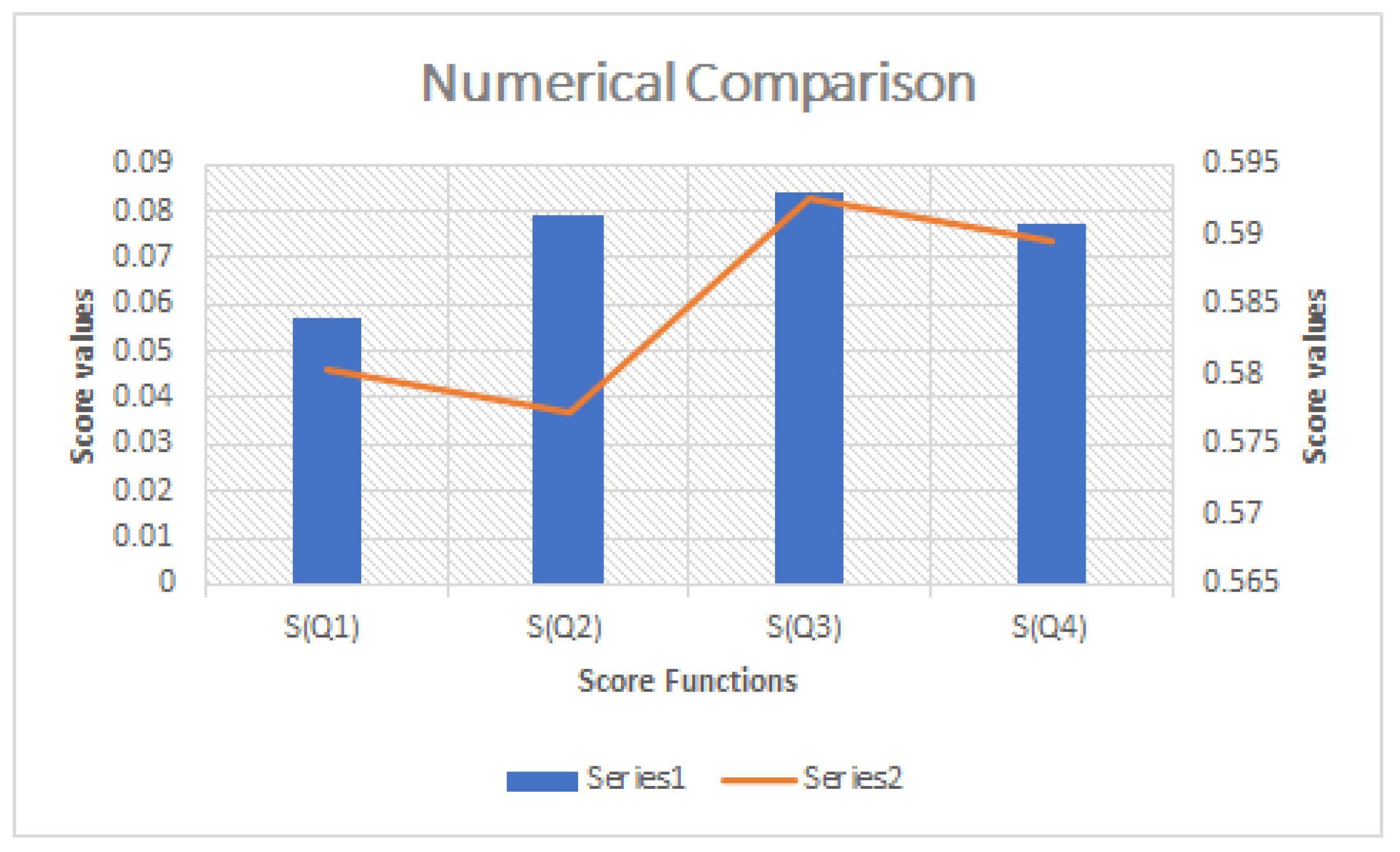
Calculate the score values for each choice using SF, and then rank the results.

Then, score function (SF) and accuracy function (AF) are given by

$$\begin{array}{ccc}\hfill Sc& =& \frac{1}{6}\left\{3+{\underline{\mathsf{\Gamma }}}_{{\top }_{\mathsf{\ell }}}/{\underline{\mathsf{\Xi }}}_{{\top }_{\mathsf{\ell }}}+{\overline{\mathsf{\Gamma }}}_{{\top }_{\mathsf{\ell }}}/{\overline{\mathsf{\Xi }}}_{{\top }_{\mathsf{\ell }}}-{\underline{\nabla }}_{{\top }_{\mathsf{\ell }}}/{\underline{\mathsf{\Lambda }}}_{{\top }_{\mathsf{\ell }}}-{\overline{\nabla }}_{{\top }_{\mathsf{\ell }}}/{\overline{\mathsf{\Lambda }}}_{{\top }_{\mathsf{\ell }}}-{\underline{\Im }}_{{\top }_{\mathsf{\ell }}}/{\underline{\mho }}_{{\top }_{\mathsf{\ell }}}-{\overline{\Im }}_{{\top }_{\mathsf{\ell }}}/{\overline{\mho }}_{{\top }_{\mathsf{\ell }}}\right\},S\in [0,1]\hfill \\ \hfill Ac& =& \frac{1}{6}\left\{3+{\underline{\mathsf{\Gamma }}}_{{\top }_{\mathsf{\ell }}}/{\underline{\mathsf{\Xi }}}_{{\top }_{\mathsf{\ell }}}+{\overline{\mathsf{\Gamma }}}_{{\top }_{\mathsf{\ell }}}/{\overline{\mathsf{\Xi }}}_{{\top }_{\mathsf{\ell }}}+{\underline{\nabla }}_{{\top }_{\mathsf{\ell }}}/{\underline{\mathsf{\Lambda }}}_{{\top }_{\mathsf{\ell }}}+{\overline{\nabla }}_{{\top }_{\mathsf{\ell }}}/{\overline{\mathsf{\Lambda }}}_{{\top }_{\mathsf{\ell }}}-{\underline{\Im }}_{{\top }_{\mathsf{\ell }}}/{\underline{\mho }}_{{\top }_{\mathsf{\ell }}}+{\overline{\Im }}_{{\top }_{\mathsf{\ell }}}/{\overline{\mho }}_{{\top }_{\mathsf{\ell }}}\right\},A\in [0,1].\hfill \end{array}$$

Case Study with Numerical Example

Case Study: The theory of “making decisions,” which is crucial to many scientific fields, was primarily created in the context of probability theory. Pattern recognition is one area where probabilistic decision-making methods frequently perform exceptionally well, but there are other situations where they fall short. When the usual probabilistic formalism is insufficient to describe the events under consideration, such as when they are not truly random, the introduction of probabilities as measurements of empirical frequencies in numerous identical experiments may lose some of their significance. The “source” of uncertainty in a decision is frequently partially or entirely deterministic. The decision-makers may decide to analyze the alternative using PSV–NHFRSs and the associated confidence levels, due to their familiarity with the evaluation. The present study used the idea of confidence levels in the aggregation process to evaluate the alternative employing PSV–NHFRSs. For this reason, we added probability information to each valued neutrosophic hesitant fuzzy rough element. To put it more simply, we considered probability, confidence level, and neutrosophy theories all at once. Evaluation professionals are frequently sought for two forms of information when dealing with practical decision-making challenges: the effectiveness of the assessment objects and understanding of the evaluation domains (called confidence levels). All of the methods in use today do not trust the expertise of the experts and only take into account positive facts. We encountered various issues in many areas of life where there was ambiguity, including engineering, economics, modelling, and medical diagnosis, among others. However, how to express and use uncertainty in mathematical modeling is commonly discussed. Researchers from all across the world have offered and suggested a variety of solutions to problems like uncertainty. Multiple attribute decision making (MADM), which enables identification of the most pertinent and distinctive solution, is the most crucial component in decision-making issues. However, in other circumstances, selecting the best course of action can be quite difficult, due to conflicting facts. Zadeh developed the concept of fuzzy sets to address and steer clear of uncertainty and ambiguity problems. Sets containing MD-components are comparable to fuzzy sets. In conventional set theory, the binary form of the bivalent condition, of whether the elements fully belong to the set, is used to analyze the MD of the set’s members. The value of set elements can now be determined using fuzzy set theory. To reflect this, the MD uses the interval [0, 1] as its effective unit interval. The classical set’s indicator function is a particular instance of that set if the fuzzy set’s MD only accepts the values 0 or 1. Thus, the fuzzy set is the classical set’s generalization. In fuzzy set theory, the conventional bivalent set is frequently referred to as the crisp set. Fuzzy set theory is applicable in many fields where information is uncertain or imperfect.

Numerical Example: Health professionals encounter several issues when treating more complex diseases as a result of complications in various diseases. For patients, doctors, and medical theory to survive, precise decision-making in the medical sector is crucial. Due to the complexity of these issues, FS theory participates in this area and has numerous applications. Figure 1 depicts a general overview of the different hesitant factors and probabilities that are effected on heart diseases. Figure 2 shows cardiac disease. The algorithm was designed on the basis of the uncertainty issues in health professions. The weight values were $\delta$$={(0.24,0.34,0.26,0.16)}^T$, and these affected the information. Where appropriate, the information was gathered from the decision modeling’s hesitancies and probabilities. As well as observing all outcomes, both positive and negative, the experts’ levels of confidence were also noted.

There are four major techniques that are used for Cardiac imaging modality given below:

${\mathsf{\Theta }}_1=$Cardiac Magnetic Resonance Imaging (MRI): Heart MRIs use radio waves and magnets to produce images of the heart, without the patient seeing or feeling anything entering the body. The components of the heart, including its chambers, valves, and muscles, as well as how effectively they are functioning and how blood is moving, can be seen on a cardiac MRI. The health-care professional can diagnose the issue and determine what is wrong thanks to these finely detailed, high-quality photographs in two or three dimensions.

${\mathsf{\Theta }}_2=$Cardiac Catheterization: In order to detect or treat some heart diseases, such as blocked arteries or irregular heartbeats, a thin, flexible tube (catheter) is guided through a blood vessel to the heart during a cardiac catheterization procedure. Doctors learn vital details about the heart’s blood arteries, heart valves, and muscle through cardiac catheterization. Doctors can perform a variety of heart tests, provide treatments, or remove a sample of heart tissue for close study during cardiac catheterization. Cardiac catheterization is used during some heart disease therapies, including coronary angioplasty and coronary stinting. In most cases, the patient is awake throughout the cardiac catheterization, but is provided with sedatives. A cardiac catheterization has a short recovery period and a low risk of complications.

${\mathsf{\Theta }}_3=$Electron-Beam Computed Tomography (EBCT): In the specific type of computed tomography (CT) known as electron beam computed tomography (EBCT), the X-ray tube is not manually spun in order to rotate the X-ray photon source. This new design was specifically created to better represent heart structures that are constantly in motion and to perform a full cycle of movement with each beat. The X-ray source-point moves in a circle in space around the object to be scanned, just like in traditional CT technology. However, in EBT, the image circle is only partially surrounded by the huge, stationary X-ray tube. The X-ray source point and electron-beam focus point are electronically moved along a tungsten anode in the tube, tracing a huge circular arc on its inner surface, as opposed to moving the tube itself. This motion may occur quite quickly. By the 2020s, multi-detector CT imagery technology had advanced so quickly that electron beam CT was no longer able to keep up.

${\mathsf{\Theta }}_4=$Echo cardiography: An echo cardiography creates images of the heart using sound waves. The doctor can watch the heart beating and pumping blood thanks to this typical test. Heart disease can be detected by the doctor using the pictures from an echo cardiography. The patient might undergo one of several different types of echo cardiogram, depending on the information the doctor needs. Most echo cardiography types carry little to no risk.

The different probabilities and hesitations are given in the above diagrams. The data was collected from the cardiac professionals.

Table 1, Table 2, Table 3 and Table 4 provides the information collected from four medical experts. Table 5 is the integrated table. Table 6 provide the information obtained by applying the CL–PSV–NHFRWA operator and the result of the PSV–NHFRWA score function is in Table 7. Table 8 provide the information obtained by applying the novel CL–PSV–NHFRWG operator. Table 9 provide the information obtained by applying the PSV–NHFRWG score function, and, then, the results obtained for current MADM.

Step 1

Table 1. Expert-1 information.

	${\widehat{C}}_1$	${\widehat{C}}_2$
${\mathsf{\Theta }}_1$	$\left[\begin{array}{c}\left[\left\{\left(\frac{0.2}{0.4},\frac{0.6}{0.6}\right),\left(\frac{0.3}{0.7},\frac{0.4}{0.3}\right),\left(\frac{0.3}{0.2},\frac{0.4}{0.3},\frac{0.6}{0.5}\right)\right\},0.4\right],\\ \\ \left[\left\{\left(\frac{0.2}{1.0}\right),\left(\frac{0.3}{0.3},\frac{0.6}{0.1},\frac{0.7}{0.6}\right),\left(\frac{0.4}{0.3},\frac{0.5}{0.4},\frac{0.1}{0.3}\right)\right\},0.6\right]\end{array}\right]$	$\left[\begin{array}{c}\left[\left\{\left(\frac{0.1}{0.3},\frac{0.5}{0.6},\frac{0.6}{0.1}\right),\left(\frac{0.8}{1.0}\right),\left(\frac{0.2}{0.1},\frac{0.1}{0.6},\frac{0.9}{0.3}\right)\right\},0.1\right],\\ \\ \left[\left\{\left(\frac{0.2}{0.4},\frac{0.6}{0.6},\frac{0.6}{0.6}\right),\left(\frac{0.2}{0.4},\frac{0.6}{0.6},\frac{0.6}{0.6}\right),\left(\frac{0.2}{0.4}\right)\right\},0.9\right]\end{array}\right]$
${\mathsf{\Theta }}_2$	$\left[\begin{array}{c}\left[\left\{\left(\frac{0.7}{0.4}\right),\left(\frac{0.1}{0.6},\frac{0.5}{0.2},\frac{0.6}{0.2}\right),\left(\frac{0.7}{0.3},\frac{0.4}{0.6},\frac{0.6}{0.1}\right)\right\},0.1\right],\\ \\ \left[\left\{\left(\frac{0.2}{0.4},\frac{0.6}{0.5},\frac{0.4}{0.1}\right),\left(\frac{0.8}{0.2},\frac{0.5}{0.8}\right),\left(\frac{0.8}{0.3},\frac{0.1}{0.7}\right)\right\},0.9\right]\end{array}\right]$	$\left[\begin{array}{c}\left[\left\{\left(\frac{0.2}{0.4},\frac{0.6}{0.6}\right),\left(\frac{0.2}{0.4},\frac{0.6}{0.6},\frac{0.6}{0.6}\right),\left(\frac{0.2}{0.4},\frac{0.6}{0.6}\right)\right\},0.2\right],\\ \\ \left[\left\{\left(\frac{0.6}{0.1},\frac{0.7}{0.9}\right),\left(\frac{0.2}{0.4},\frac{0.6}{0.6}\right),\left(\frac{0.2}{0.7},\frac{0.6}{0.3}\right)\right\},0.8\right]\end{array}\right]$
${\mathsf{\Theta }}_3$	$\left[\begin{array}{c}\left[\left\{\left(\frac{0.4}{0.1},\frac{0.6}{0.2},\frac{0.2}{0.7}\right),\left(\frac{0.8}{0.4},\frac{0.6}{0.6},\frac{0.1}{0.6}\right),\left(\frac{0.2}{1.0}\right)\right\},0.3\right],\\ \\ \left[\left\{\left(\frac{0.2}{0.4},\frac{0.6}{0.6}\right),\left(\frac{0.2}{0.4},\frac{0.6}{0.6}\right),\left(\frac{0.2}{0.4},\frac{0.6}{0.1},\frac{0.6}{0.5}\right)\right\},0.7\right]\end{array}\right]$	$\left[\begin{array}{c}\left[\left\{\left(\frac{0.2}{0.4},\frac{0.6}{0.6}\right),\left(\frac{0.2}{0.4},\frac{0.6}{0.6},\frac{0.6}{0.6}\right),\left(\frac{0.2}{0.4},\frac{0.6}{0.6}\right)\right\},0.7\right],\\ \\ \left[\left\{\left(\frac{0.9}{1.0}\right),\left(\frac{0.2}{0.4},\frac{0.6}{0.2},\frac{0.2}{0.4}\right),\left(\frac{0.2}{0.7},\frac{0.7}{0.2},\frac{0.6}{0.1}\right)\right\},0.3\right]\end{array}\right]$
${\mathsf{\Theta }}_4$	$\left[\begin{array}{c}\left[\left\{\left(\frac{0.2}{0.2},\frac{0.1}{0.2},\frac{0.6}{0.6}\right),\left(\frac{0.2}{1.0}\right),\left(\frac{0.4}{0.1},\frac{0.6}{0.6},\frac{0.1}{0.3}\right)\right\},0.5\right],\\ \\ \left[\left\{\left(\frac{0.4}{0.8},\frac{0.6}{0.2}\right),\left(\frac{0.2}{0.2},\frac{0.1}{0.5},\frac{0.6}{0.3}\right),\left(\frac{0.3}{0.8},\frac{0.7}{0.2}\right)\right\},0.5\right]\end{array}\right]$	$\left[\begin{array}{c}\left[\left\{\left(\frac{0.2}{0.4},\frac{0.6}{0.6}\right),\left(\frac{0.2}{0.4}\right),\left(\frac{0.2}{0.4},\frac{0.6}{0.6},\frac{0.6}{0.6},\frac{0.6}{0.6}\right)\right\},0.2\right],\\ \\ \left[\left\{\left(\frac{0.7}{0.2},\frac{0.6}{0.8}\right),\left(\frac{0.1}{0.4},\frac{0.5}{0.1},\frac{0.6}{0.5}\right),\left(\frac{0.2}{1.0}\right)\right\},0.8\right]\end{array}\right]$
	${\widehat{C}}_3$	${\widehat{C}}_4$
${\mathsf{\Theta }}_1$	$\left[\begin{array}{c}\left[\left\{\left(\frac{0.1}{0.7},\frac{0.4}{0.3}\right),\left(\frac{0.8}{1.0}\right),\left(\frac{0.3}{0.7},\frac{0.4}{0.1},\frac{0.6}{0.2}\right)\right\},0.2\right],\\ \\ \left[\left\{\left(\frac{0.2}{1.0}\right),\left(\frac{0.3}{0.3},\frac{0.6}{0.1},\frac{0.7}{0.6}\right),\left(\frac{0.4}{0.3},\frac{0.5}{0.4},\frac{0.1}{0.3}\right)\right\},0.8\right]\end{array}\right]$	$\left[\begin{array}{c}\left[\left\{\left(\frac{0.2}{0.4},\frac{0.6}{0.6}\right),\left(\frac{0.3}{0.7},\frac{0.4}{0.3}\right),\left(\frac{0.3}{0.2},\frac{0.4}{0.3},\frac{0.6}{0.5}\right)\right\},0.4\right],\\ \\ \left[\left\{\left(\frac{0.2}{1.0}\right),\left(\frac{0.3}{0.3},\frac{0.6}{0.1},\frac{0.7}{0.6}\right),\left(\frac{0.4}{0.3},\frac{0.5}{0.4},\frac{0.1}{0.3}\right)\right\},0.6\right]\end{array}\right]$
${\mathsf{\Theta }}_2$	$\left[\begin{array}{c}\left[\left\{\left(\frac{0.2}{0.3},\frac{0.6}{0.6},\frac{0.6}{0.1}\right),\left(\frac{0.2}{0.7},\frac{0.5}{0.2},\frac{0.4}{0.1}\right),\left(\frac{0.7}{0.4}\right)\right\},0.6\right],\\ \\ \left[\left\{\left(\frac{0.2}{0.4},\frac{0.6}{0.5},\frac{0.4}{0.1}\right),\left(\frac{0.8}{0.2},\frac{0.5}{0.8}\right),\left(\frac{0.8}{0.3},\frac{0.1}{0.7}\right)\right\},0.4\right]\end{array}\right]$	$\left[\begin{array}{c}\left[\left\{\left(\frac{0.7}{0.4}\right),\left(\frac{0.1}{0.6},\frac{0.5}{0.2},\frac{0.6}{0.2}\right),\left(\frac{0.7}{0.3},\frac{0.4}{0.6},\frac{0.6}{0.1}\right)\right\},0.1\right],\\ \\ \left[\left\{\left(\frac{0.2}{0.4},\frac{0.6}{0.5},\frac{0.4}{0.1}\right),\left(\frac{0.8}{0.2},\frac{0.5}{0.8}\right),\left(\frac{0.8}{0.3},\frac{0.1}{0.7}\right)\right\},0.9\right]\end{array}\right]$
${\mathsf{\Theta }}_3$	$\left[\begin{array}{c}\left[\left\{\left(\frac{0.3}{0.1},\frac{0.4}{0.2},\frac{0.2}{0.7}\right),\left(\frac{0.2}{1.0}\right),\left(\frac{0.8}{0.4},\frac{0.6}{0.3},\frac{0.1}{0.3}\right)\right\},0.1\right],\\ \\ \left[\left\{\left(\frac{0.2}{0.4},\frac{0.6}{0.6}\right),\left(\frac{0.2}{0.4},\frac{0.6}{0.6}\right),\left(\frac{0.2}{0.4},\frac{0.6}{0.5},\frac{0.6}{0.1}\right)\right\},0.9\right]\end{array}\right]$	$\left[\begin{array}{c}\left[\left\{\left(\frac{0.4}{0.1},\frac{0.6}{0.2},\frac{0.2}{0.7}\right),\left(\frac{0.1}{0.4},\frac{0.9}{0.2},\frac{0.5}{0.2}\right),\left(\frac{0.2}{1.0}\right)\right\},0.1\right],\\ \\ \left[\left\{\left(\frac{0.2}{0.4},\frac{0.6}{0.6}\right),\left(\frac{0.2}{0.4},\frac{0.6}{0.6}\right),\left(\frac{0.2}{0.4},\frac{0.6}{0.6},\frac{0.6}{0.6}\right)\right\},0.9\right]\end{array}\right]$
${\mathsf{\Theta }}_4$	$\left[\begin{array}{c}\left[\left\{\left(\frac{0.9}{1.0}\right),\left(\frac{0.3}{0.2},\frac{0.2}{0.2},\frac{0.6}{0.6}\right),\left(\frac{0.4}{0.1},\frac{0.6}{0.6},\frac{0.1}{0.3}\right)\right\},0.2\right],\\ \\ \left[\left\{\left(\frac{0.4}{0.8},\frac{0.6}{0.2}\right),\left(\frac{0.2}{0.2},\frac{0.1}{0.5},\frac{0.6}{0.3}\right),\left(\frac{0.3}{0.8},\frac{0.7}{0.2}\right)\right\},0.8\right]\end{array}\right]$	$\left[\begin{array}{c}\left[\left\{\left(\frac{0.2}{0.2},\frac{0.1}{0.2},\frac{0.6}{0.6}\right),\left(\frac{0.2}{1.0}\right),\left(\frac{0.4}{0.1},\frac{0.6}{0.6},\frac{0.1}{0.3}\right)\right\},0.3\right],\\ \\ \left[\left\{\left(\frac{0.4}{0.8},\frac{0.6}{0.2}\right),\left(\frac{0.2}{0.2},\frac{0.1}{0.5},\frac{0.6}{0.3}\right),\left(\frac{0.3}{0.8},\frac{0.7}{0.2}\right)\right\},0.7\right]\end{array}\right]$

Table 1. Expert-1 information.

	${\widehat{C}}_1$	${\widehat{C}}_2$
${\mathsf{\Theta }}_1$	$\left[\begin{array}{c}\left[\left\{\left(\frac{0.2}{0.4},\frac{0.6}{0.6}\right),\left(\frac{0.3}{0.7},\frac{0.4}{0.3}\right),\left(\frac{0.3}{0.2},\frac{0.4}{0.3},\frac{0.6}{0.5}\right)\right\},0.4\right],\\ \\ \left[\left\{\left(\frac{0.2}{1.0}\right),\left(\frac{0.3}{0.3},\frac{0.6}{0.1},\frac{0.7}{0.6}\right),\left(\frac{0.4}{0.3},\frac{0.5}{0.4},\frac{0.1}{0.3}\right)\right\},0.6\right]\end{array}\right]$	$\left[\begin{array}{c}\left[\left\{\left(\frac{0.1}{0.3},\frac{0.5}{0.6},\frac{0.6}{0.1}\right),\left(\frac{0.8}{1.0}\right),\left(\frac{0.2}{0.1},\frac{0.1}{0.6},\frac{0.9}{0.3}\right)\right\},0.1\right],\\ \\ \left[\left\{\left(\frac{0.2}{0.4},\frac{0.6}{0.6},\frac{0.6}{0.6}\right),\left(\frac{0.2}{0.4},\frac{0.6}{0.6},\frac{0.6}{0.6}\right),\left(\frac{0.2}{0.4}\right)\right\},0.9\right]\end{array}\right]$
${\mathsf{\Theta }}_2$	$\left[\begin{array}{c}\left[\left\{\left(\frac{0.7}{0.4}\right),\left(\frac{0.1}{0.6},\frac{0.5}{0.2},\frac{0.6}{0.2}\right),\left(\frac{0.7}{0.3},\frac{0.4}{0.6},\frac{0.6}{0.1}\right)\right\},0.1\right],\\ \\ \left[\left\{\left(\frac{0.2}{0.4},\frac{0.6}{0.5},\frac{0.4}{0.1}\right),\left(\frac{0.8}{0.2},\frac{0.5}{0.8}\right),\left(\frac{0.8}{0.3},\frac{0.1}{0.7}\right)\right\},0.9\right]\end{array}\right]$	$\left[\begin{array}{c}\left[\left\{\left(\frac{0.2}{0.4},\frac{0.6}{0.6}\right),\left(\frac{0.2}{0.4},\frac{0.6}{0.6},\frac{0.6}{0.6}\right),\left(\frac{0.2}{0.4},\frac{0.6}{0.6}\right)\right\},0.2\right],\\ \\ \left[\left\{\left(\frac{0.6}{0.1},\frac{0.7}{0.9}\right),\left(\frac{0.2}{0.4},\frac{0.6}{0.6}\right),\left(\frac{0.2}{0.7},\frac{0.6}{0.3}\right)\right\},0.8\right]\end{array}\right]$
${\mathsf{\Theta }}_3$	$\left[\begin{array}{c}\left[\left\{\left(\frac{0.4}{0.1},\frac{0.6}{0.2},\frac{0.2}{0.7}\right),\left(\frac{0.8}{0.4},\frac{0.6}{0.6},\frac{0.1}{0.6}\right),\left(\frac{0.2}{1.0}\right)\right\},0.3\right],\\ \\ \left[\left\{\left(\frac{0.2}{0.4},\frac{0.6}{0.6}\right),\left(\frac{0.2}{0.4},\frac{0.6}{0.6}\right),\left(\frac{0.2}{0.4},\frac{0.6}{0.1},\frac{0.6}{0.5}\right)\right\},0.7\right]\end{array}\right]$	$\left[\begin{array}{c}\left[\left\{\left(\frac{0.2}{0.4},\frac{0.6}{0.6}\right),\left(\frac{0.2}{0.4},\frac{0.6}{0.6},\frac{0.6}{0.6}\right),\left(\frac{0.2}{0.4},\frac{0.6}{0.6}\right)\right\},0.7\right],\\ \\ \left[\left\{\left(\frac{0.9}{1.0}\right),\left(\frac{0.2}{0.4},\frac{0.6}{0.2},\frac{0.2}{0.4}\right),\left(\frac{0.2}{0.7},\frac{0.7}{0.2},\frac{0.6}{0.1}\right)\right\},0.3\right]\end{array}\right]$
${\mathsf{\Theta }}_4$	$\left[\begin{array}{c}\left[\left\{\left(\frac{0.2}{0.2},\frac{0.1}{0.2},\frac{0.6}{0.6}\right),\left(\frac{0.2}{1.0}\right),\left(\frac{0.4}{0.1},\frac{0.6}{0.6},\frac{0.1}{0.3}\right)\right\},0.5\right],\\ \\ \left[\left\{\left(\frac{0.4}{0.8},\frac{0.6}{0.2}\right),\left(\frac{0.2}{0.2},\frac{0.1}{0.5},\frac{0.6}{0.3}\right),\left(\frac{0.3}{0.8},\frac{0.7}{0.2}\right)\right\},0.5\right]\end{array}\right]$	$\left[\begin{array}{c}\left[\left\{\left(\frac{0.2}{0.4},\frac{0.6}{0.6}\right),\left(\frac{0.2}{0.4}\right),\left(\frac{0.2}{0.4},\frac{0.6}{0.6},\frac{0.6}{0.6},\frac{0.6}{0.6}\right)\right\},0.2\right],\\ \\ \left[\left\{\left(\frac{0.7}{0.2},\frac{0.6}{0.8}\right),\left(\frac{0.1}{0.4},\frac{0.5}{0.1},\frac{0.6}{0.5}\right),\left(\frac{0.2}{1.0}\right)\right\},0.8\right]\end{array}\right]$
	${\widehat{C}}_3$	${\widehat{C}}_4$
${\mathsf{\Theta }}_1$	$\left[\begin{array}{c}\left[\left\{\left(\frac{0.1}{0.7},\frac{0.4}{0.3}\right),\left(\frac{0.8}{1.0}\right),\left(\frac{0.3}{0.7},\frac{0.4}{0.1},\frac{0.6}{0.2}\right)\right\},0.2\right],\\ \\ \left[\left\{\left(\frac{0.2}{1.0}\right),\left(\frac{0.3}{0.3},\frac{0.6}{0.1},\frac{0.7}{0.6}\right),\left(\frac{0.4}{0.3},\frac{0.5}{0.4},\frac{0.1}{0.3}\right)\right\},0.8\right]\end{array}\right]$	$\left[\begin{array}{c}\left[\left\{\left(\frac{0.2}{0.4},\frac{0.6}{0.6}\right),\left(\frac{0.3}{0.7},\frac{0.4}{0.3}\right),\left(\frac{0.3}{0.2},\frac{0.4}{0.3},\frac{0.6}{0.5}\right)\right\},0.4\right],\\ \\ \left[\left\{\left(\frac{0.2}{1.0}\right),\left(\frac{0.3}{0.3},\frac{0.6}{0.1},\frac{0.7}{0.6}\right),\left(\frac{0.4}{0.3},\frac{0.5}{0.4},\frac{0.1}{0.3}\right)\right\},0.6\right]\end{array}\right]$
${\mathsf{\Theta }}_2$	$\left[\begin{array}{c}\left[\left\{\left(\frac{0.2}{0.3},\frac{0.6}{0.6},\frac{0.6}{0.1}\right),\left(\frac{0.2}{0.7},\frac{0.5}{0.2},\frac{0.4}{0.1}\right),\left(\frac{0.7}{0.4}\right)\right\},0.6\right],\\ \\ \left[\left\{\left(\frac{0.2}{0.4},\frac{0.6}{0.5},\frac{0.4}{0.1}\right),\left(\frac{0.8}{0.2},\frac{0.5}{0.8}\right),\left(\frac{0.8}{0.3},\frac{0.1}{0.7}\right)\right\},0.4\right]\end{array}\right]$	$\left[\begin{array}{c}\left[\left\{\left(\frac{0.7}{0.4}\right),\left(\frac{0.1}{0.6},\frac{0.5}{0.2},\frac{0.6}{0.2}\right),\left(\frac{0.7}{0.3},\frac{0.4}{0.6},\frac{0.6}{0.1}\right)\right\},0.1\right],\\ \\ \left[\left\{\left(\frac{0.2}{0.4},\frac{0.6}{0.5},\frac{0.4}{0.1}\right),\left(\frac{0.8}{0.2},\frac{0.5}{0.8}\right),\left(\frac{0.8}{0.3},\frac{0.1}{0.7}\right)\right\},0.9\right]\end{array}\right]$
${\mathsf{\Theta }}_3$	$\left[\begin{array}{c}\left[\left\{\left(\frac{0.3}{0.1},\frac{0.4}{0.2},\frac{0.2}{0.7}\right),\left(\frac{0.2}{1.0}\right),\left(\frac{0.8}{0.4},\frac{0.6}{0.3},\frac{0.1}{0.3}\right)\right\},0.1\right],\\ \\ \left[\left\{\left(\frac{0.2}{0.4},\frac{0.6}{0.6}\right),\left(\frac{0.2}{0.4},\frac{0.6}{0.6}\right),\left(\frac{0.2}{0.4},\frac{0.6}{0.5},\frac{0.6}{0.1}\right)\right\},0.9\right]\end{array}\right]$	$\left[\begin{array}{c}\left[\left\{\left(\frac{0.4}{0.1},\frac{0.6}{0.2},\frac{0.2}{0.7}\right),\left(\frac{0.1}{0.4},\frac{0.9}{0.2},\frac{0.5}{0.2}\right),\left(\frac{0.2}{1.0}\right)\right\},0.1\right],\\ \\ \left[\left\{\left(\frac{0.2}{0.4},\frac{0.6}{0.6}\right),\left(\frac{0.2}{0.4},\frac{0.6}{0.6}\right),\left(\frac{0.2}{0.4},\frac{0.6}{0.6},\frac{0.6}{0.6}\right)\right\},0.9\right]\end{array}\right]$
${\mathsf{\Theta }}_4$	$\left[\begin{array}{c}\left[\left\{\left(\frac{0.9}{1.0}\right),\left(\frac{0.3}{0.2},\frac{0.2}{0.2},\frac{0.6}{0.6}\right),\left(\frac{0.4}{0.1},\frac{0.6}{0.6},\frac{0.1}{0.3}\right)\right\},0.2\right],\\ \\ \left[\left\{\left(\frac{0.4}{0.8},\frac{0.6}{0.2}\right),\left(\frac{0.2}{0.2},\frac{0.1}{0.5},\frac{0.6}{0.3}\right),\left(\frac{0.3}{0.8},\frac{0.7}{0.2}\right)\right\},0.8\right]\end{array}\right]$	$\left[\begin{array}{c}\left[\left\{\left(\frac{0.2}{0.2},\frac{0.1}{0.2},\frac{0.6}{0.6}\right),\left(\frac{0.2}{1.0}\right),\left(\frac{0.4}{0.1},\frac{0.6}{0.6},\frac{0.1}{0.3}\right)\right\},0.3\right],\\ \\ \left[\left\{\left(\frac{0.4}{0.8},\frac{0.6}{0.2}\right),\left(\frac{0.2}{0.2},\frac{0.1}{0.5},\frac{0.6}{0.3}\right),\left(\frac{0.3}{0.8},\frac{0.7}{0.2}\right)\right\},0.7\right]\end{array}\right]$

Table 2. Expert-2 information.

	${\widehat{C}}_1$	${\widehat{C}}_2$
${\mathsf{\Theta }}_1$	$\left[\begin{array}{c}\left[\left\{\left(\frac{0.7}{1.0}\right),\left(\frac{0.1}{0.2},\frac{0.5}{0.8}\right),\left(\frac{0.3}{0.3},\frac{0.4}{0.1},\frac{0.9}{0.6}\right)\right\},0.7\right],\\ \\ \left[\left\{\left(\frac{0.9}{1.0}\right),\left(\frac{0.3}{0.1},\frac{0.5}{0.2},\frac{0.7}{0.6}\right),\left(\frac{0.4}{0.1},\frac{0.5}{0.4},\frac{0.4}{0.5}\right)\right\},0.3\right]\end{array}\right]$	$\left[\begin{array}{c}\left[\left\{\left(\frac{0.1}{0.4},\frac{0.9}{0.6}\right),\left(\frac{0.3}{0.7},\frac{0.4}{0.3}\right),\left(\frac{0.3}{0.1},\frac{0.5}{0.3},\frac{0.6}{0.6}\right)\right\},0.7\right],\\ \\ \left[\left\{\left(\frac{0.3}{0.3},\frac{0.2}{0.1},\frac{0.9}{0.6}\right),\left(\frac{0.8}{1.0}\right),\left(\frac{0.3}{0.7},\frac{0.5}{0.2},\frac{0.3}{0.1}\right)\right\},0.3\right]\end{array}\right]$
${\mathsf{\Theta }}_2$	$\left[\begin{array}{c}\left[\left\{\left(\frac{0.2}{0.3},\frac{0.6}{0.6},\frac{0.6}{0.1}\right),\left(\frac{0.2}{0.7},\frac{0.5}{0.2},\frac{0.4}{0.1}\right),\left(\frac{0.7}{0.4}\right)\right\},0.1\right],\\ \\ \left[\left\{\left(\frac{0.5}{0.4},\frac{0.6}{0.4},\frac{0.2}{0.2}\right),\left(\frac{0.9}{0.1},\frac{0.5}{0.9}\right),\left(\frac{0.8}{0.3},\frac{0.1}{0.7}\right)\right\},0.9\right]\end{array}\right]$	$\left[\begin{array}{c}\left[\left\{\left(\frac{0.7}{0.4}\right),\left(\frac{0.1}{0.6},\frac{0.5}{0.2},\frac{0.6}{0.2}\right),\left(\frac{0.7}{0.3},\frac{0.4}{0.6},\frac{0.6}{0.1}\right)\right\},0.2\right],\\ \\ \left[\left\{\left(\frac{0.2}{0.4},\frac{0.6}{0.5},\frac{0.4}{0.1}\right),\left(\frac{0.7}{1.0}\right),\left(\frac{0.8}{1.0}\right)\right\},0.8\right]\end{array}\right]$
${\mathsf{\Theta }}_3$	$\left[\begin{array}{c}\left[\left\{\left(\frac{0.3}{0.1},\frac{0.4}{0.2},\frac{0.2}{0.7}\right),\left(\frac{0.2}{1.0}\right),\left(\frac{0.8}{0.4},\frac{0.6}{0.3},\frac{0.1}{0.3}\right)\right\},0.5\right],\\ \\ \left[\left\{\left(\frac{0.2}{0.4},\frac{0.5}{0.6}\right),\left(\frac{0.2}{0.3},\frac{0.5}{0.7}\right),\left(\frac{0.2}{0.3},\frac{0.1}{0.6},\frac{0.6}{0.1}\right)\right\},0.5\right]\end{array}\right]$	$\left[\begin{array}{c}\left[\left\{\left(\frac{0.5}{1.0}\right),\left(\frac{0.1}{0.3},\frac{0.8}{0.4},\frac{0.3}{0.3}\right),\left(\frac{0.2}{1.0}\right)\right\},0.4\right],\\ \\ \left[\left\{\left(\frac{0.7}{0.5},\frac{0.2}{0.5}\right),\left(\frac{0.2}{0.4},\frac{0.6}{0.3},\frac{0.2}{0.3}\right),\left(\frac{0.2}{0.1},\frac{0.6}{0.9}\right)\right\},0.6\right]\end{array}\right]$
${\mathsf{\Theta }}_4$	$\left[\begin{array}{c}\left[\left\{\left(\frac{0.9}{1.0}\right),\left(\frac{0.3}{0.1},\frac{0.6}{0.7},\frac{0.7}{0.2}\right),\left(\frac{0.3}{0.2},\frac{0.2}{0.2},\frac{0.6}{0.6}\right)\right\},0.2\right],\\ \\ \left[\left\{\left(\frac{0.4}{0.9},\frac{0.6}{0.1}\right),\left(\frac{0.2}{0.3},\frac{0.1}{0.4},\frac{0.5}{0.3}\right),\left(\frac{0.3}{0.8},\frac{0.7}{0.2}\right)\right\},0.8\right]\end{array}\right]$	$\left[\begin{array}{c}\left[\left\{\left(\frac{0.2}{0.2},\frac{0.1}{0.2},\frac{0.6}{0.6}\right),\left(\frac{0.2}{1.0}\right),\left(\frac{0.4}{0.1},\frac{0.6}{0.6},\frac{0.1}{0.3}\right)\right\},0.3\right],\\ \\ \left[\left\{\left(\frac{0.4}{0.8},\frac{0.6}{0.2}\right),\left(\frac{0.2}{0.2},\frac{0.2}{0.7},\frac{0.6}{0.1}\right),,\left(\frac{0.2}{1.0}\right)\right\},0.7\right]\end{array}\right]$
	${\widehat{C}}_3$	${\widehat{C}}_4$
${\mathsf{\Theta }}_1$	$\left[\begin{array}{c}\left[\left\{\left(\frac{0.2}{0.2},\frac{0.4}{0.8}\right),\left(\frac{0.2}{0.7},\frac{0.5}{0.3}\right),\left(\frac{0.3}{0.7},\frac{0.4}{0.1},\frac{0.6}{0.2}\right)\right\},0.2\right],\\ \\ \left[\left\{\left(\frac{0.2}{1.0}\right),\left(\frac{0.3}{0.3},\frac{0.6}{0.1},\frac{0.7}{0.6}\right),\left(\frac{0.4}{0.3},\frac{0.5}{0.4},\frac{0.1}{0.3}\right)\right\},0.8\right]\end{array}\right]$	$\left[\begin{array}{c}\left[\left\{\left(\frac{0.3}{0.4},\frac{0.6}{0.6}\right),\left(\frac{0.8}{1.0}\right),\left(\frac{0.1}{0.2},\frac{0.4}{0.6},\frac{0.6}{0.2}\right)\right\},0.1\right],\\ \\ \left[\left\{\left(\frac{0.2}{1.0}\right),\left(\frac{0.2}{0.7},\frac{0.5}{0.2},\frac{0.4}{0.1}\right),\left(\frac{0.4}{0.3},\frac{0.5}{0.4},\frac{0.1}{0.3}\right)\right\},0.9\right]\end{array}\right]$
${\mathsf{\Theta }}_2$	$\left[\begin{array}{c}\left[\left\{\left(\frac{0.2}{0.3},\frac{0.6}{0.6},\frac{0.6}{0.1}\right),\left(\frac{0.2}{0.7},\frac{0.5}{0.2},\frac{0.4}{0.1}\right),\left(\frac{0.7}{0.4}\right)\right\},0.6\right],\\ \\ \left[\left\{\left(\frac{0.2}{0.4},\frac{0.4}{0.6}\right),\left(\frac{0.8}{0.2},\frac{0.5}{0.8}\right),\left(\frac{0.2}{0.3},\frac{0.6}{0.6},\frac{0.6}{0.1}\right)\right\},0.4\right]\end{array}\right]$	$\left[\begin{array}{c}\left[\left\{\left(\frac{0.7}{1.0}\right),\left(\frac{0.1}{1.0}\right),\left(\frac{0.7}{0.3},\frac{0.3}{0.6},\frac{0.6}{0.1}\right)\right\},0.3\right],\\ \\ \left[\left\{\left(\frac{0.2}{0.4},\frac{0.6}{0.5},\frac{0.4}{0.1}\right),\left(\frac{0.8}{0.2},\frac{0.5}{0.8}\right),\left(\frac{0.8}{0.3},\frac{0.1}{0.7}\right)\right\},0.7\right]\end{array}\right]$
${\mathsf{\Theta }}_3$	$\left[\begin{array}{c}\left[\left\{\left(\frac{0.3}{1.0}\right),\left(\frac{0.2}{1.0}\right),\left(\frac{0.8}{0.4},\frac{0.6}{0.3},\frac{0.1}{0.3}\right)\right\},0.1\right],\\ \\ \left[\left\{\left(\frac{0.3}{0.2},\frac{0.2}{0.8}\right),\left(\frac{0.2}{0.4},\frac{0.6}{0.6}\right),\left(\frac{0.2}{0.4},\frac{0.6}{0.5},\frac{0.6}{0.1}\right)\right\},0.9\right]\end{array}\right]$	$\left[\begin{array}{c}\left[\left\{\left(\frac{0.4}{0.1},\frac{0.6}{0.2},\frac{0.2}{0.7}\right),\left(\frac{0.1}{0.4},\frac{0.9}{0.2},\frac{0.5}{0.2}\right),\left(\frac{0.2}{1.0}\right)\right\},0.5\right],\\ \\ \left[\left\{\left(\frac{0.8}{0.2},\frac{0.6}{0.8}\right),\left(\frac{0.4}{1.0}\right),\left(\frac{0.2}{0.4},\frac{0.6}{0.1},\frac{0.6}{0.5}\right)\right\},0.5\right]\end{array}\right]$
${\mathsf{\Theta }}_4$	$\left[\begin{array}{c}\left[\left\{\left(\frac{0.9}{1.0}\right),\left(\frac{0.3}{0.2},\frac{0.2}{0.2},\frac{0.6}{0.6}\right),\left(\frac{0.9}{1.0}\right)\right\},0.2\right],\\ \\ \left[\left\{\left(\frac{0.4}{0.8},\frac{0.6}{0.2}\right),\left(\frac{0.2}{0.2},\frac{0.1}{0.5},\frac{0.6}{0.3}\right),\left(\frac{0.3}{0.8},\frac{0.7}{0.2}\right)\right\},0.8\right]\end{array}\right]$	$\left[\begin{array}{c}\left[\left\{\left(\frac{0.2}{0.2},\frac{0.1}{0.2},\frac{0.6}{0.6}\right),\left(\frac{0.2}{1.0}\right),\left(\frac{0.4}{0.1},\frac{0.6}{0.6},\frac{0.1}{0.3}\right)\right\},0.4\right],\\ \\ \left[\left\{\left(\frac{0.4}{0.8},\frac{0.6}{0.2}\right),\left(\frac{0.5}{1.0}\right),\left(\frac{0.3}{0.8},\frac{0.7}{0.2}\right)\right\},0.6\right]\end{array}\right]$

Table 2. Expert-2 information.

	${\widehat{C}}_1$	${\widehat{C}}_2$
${\mathsf{\Theta }}_1$	$\left[\begin{array}{c}\left[\left\{\left(\frac{0.7}{1.0}\right),\left(\frac{0.1}{0.2},\frac{0.5}{0.8}\right),\left(\frac{0.3}{0.3},\frac{0.4}{0.1},\frac{0.9}{0.6}\right)\right\},0.7\right],\\ \\ \left[\left\{\left(\frac{0.9}{1.0}\right),\left(\frac{0.3}{0.1},\frac{0.5}{0.2},\frac{0.7}{0.6}\right),\left(\frac{0.4}{0.1},\frac{0.5}{0.4},\frac{0.4}{0.5}\right)\right\},0.3\right]\end{array}\right]$	$\left[\begin{array}{c}\left[\left\{\left(\frac{0.1}{0.4},\frac{0.9}{0.6}\right),\left(\frac{0.3}{0.7},\frac{0.4}{0.3}\right),\left(\frac{0.3}{0.1},\frac{0.5}{0.3},\frac{0.6}{0.6}\right)\right\},0.7\right],\\ \\ \left[\left\{\left(\frac{0.3}{0.3},\frac{0.2}{0.1},\frac{0.9}{0.6}\right),\left(\frac{0.8}{1.0}\right),\left(\frac{0.3}{0.7},\frac{0.5}{0.2},\frac{0.3}{0.1}\right)\right\},0.3\right]\end{array}\right]$
${\mathsf{\Theta }}_2$	$\left[\begin{array}{c}\left[\left\{\left(\frac{0.2}{0.3},\frac{0.6}{0.6},\frac{0.6}{0.1}\right),\left(\frac{0.2}{0.7},\frac{0.5}{0.2},\frac{0.4}{0.1}\right),\left(\frac{0.7}{0.4}\right)\right\},0.1\right],\\ \\ \left[\left\{\left(\frac{0.5}{0.4},\frac{0.6}{0.4},\frac{0.2}{0.2}\right),\left(\frac{0.9}{0.1},\frac{0.5}{0.9}\right),\left(\frac{0.8}{0.3},\frac{0.1}{0.7}\right)\right\},0.9\right]\end{array}\right]$	$\left[\begin{array}{c}\left[\left\{\left(\frac{0.7}{0.4}\right),\left(\frac{0.1}{0.6},\frac{0.5}{0.2},\frac{0.6}{0.2}\right),\left(\frac{0.7}{0.3},\frac{0.4}{0.6},\frac{0.6}{0.1}\right)\right\},0.2\right],\\ \\ \left[\left\{\left(\frac{0.2}{0.4},\frac{0.6}{0.5},\frac{0.4}{0.1}\right),\left(\frac{0.7}{1.0}\right),\left(\frac{0.8}{1.0}\right)\right\},0.8\right]\end{array}\right]$
${\mathsf{\Theta }}_3$	$\left[\begin{array}{c}\left[\left\{\left(\frac{0.3}{0.1},\frac{0.4}{0.2},\frac{0.2}{0.7}\right),\left(\frac{0.2}{1.0}\right),\left(\frac{0.8}{0.4},\frac{0.6}{0.3},\frac{0.1}{0.3}\right)\right\},0.5\right],\\ \\ \left[\left\{\left(\frac{0.2}{0.4},\frac{0.5}{0.6}\right),\left(\frac{0.2}{0.3},\frac{0.5}{0.7}\right),\left(\frac{0.2}{0.3},\frac{0.1}{0.6},\frac{0.6}{0.1}\right)\right\},0.5\right]\end{array}\right]$	$\left[\begin{array}{c}\left[\left\{\left(\frac{0.5}{1.0}\right),\left(\frac{0.1}{0.3},\frac{0.8}{0.4},\frac{0.3}{0.3}\right),\left(\frac{0.2}{1.0}\right)\right\},0.4\right],\\ \\ \left[\left\{\left(\frac{0.7}{0.5},\frac{0.2}{0.5}\right),\left(\frac{0.2}{0.4},\frac{0.6}{0.3},\frac{0.2}{0.3}\right),\left(\frac{0.2}{0.1},\frac{0.6}{0.9}\right)\right\},0.6\right]\end{array}\right]$
${\mathsf{\Theta }}_4$	$\left[\begin{array}{c}\left[\left\{\left(\frac{0.9}{1.0}\right),\left(\frac{0.3}{0.1},\frac{0.6}{0.7},\frac{0.7}{0.2}\right),\left(\frac{0.3}{0.2},\frac{0.2}{0.2},\frac{0.6}{0.6}\right)\right\},0.2\right],\\ \\ \left[\left\{\left(\frac{0.4}{0.9},\frac{0.6}{0.1}\right),\left(\frac{0.2}{0.3},\frac{0.1}{0.4},\frac{0.5}{0.3}\right),\left(\frac{0.3}{0.8},\frac{0.7}{0.2}\right)\right\},0.8\right]\end{array}\right]$	$\left[\begin{array}{c}\left[\left\{\left(\frac{0.2}{0.2},\frac{0.1}{0.2},\frac{0.6}{0.6}\right),\left(\frac{0.2}{1.0}\right),\left(\frac{0.4}{0.1},\frac{0.6}{0.6},\frac{0.1}{0.3}\right)\right\},0.3\right],\\ \\ \left[\left\{\left(\frac{0.4}{0.8},\frac{0.6}{0.2}\right),\left(\frac{0.2}{0.2},\frac{0.2}{0.7},\frac{0.6}{0.1}\right),,\left(\frac{0.2}{1.0}\right)\right\},0.7\right]\end{array}\right]$
	${\widehat{C}}_3$	${\widehat{C}}_4$
${\mathsf{\Theta }}_1$	$\left[\begin{array}{c}\left[\left\{\left(\frac{0.2}{0.2},\frac{0.4}{0.8}\right),\left(\frac{0.2}{0.7},\frac{0.5}{0.3}\right),\left(\frac{0.3}{0.7},\frac{0.4}{0.1},\frac{0.6}{0.2}\right)\right\},0.2\right],\\ \\ \left[\left\{\left(\frac{0.2}{1.0}\right),\left(\frac{0.3}{0.3},\frac{0.6}{0.1},\frac{0.7}{0.6}\right),\left(\frac{0.4}{0.3},\frac{0.5}{0.4},\frac{0.1}{0.3}\right)\right\},0.8\right]\end{array}\right]$	$\left[\begin{array}{c}\left[\left\{\left(\frac{0.3}{0.4},\frac{0.6}{0.6}\right),\left(\frac{0.8}{1.0}\right),\left(\frac{0.1}{0.2},\frac{0.4}{0.6},\frac{0.6}{0.2}\right)\right\},0.1\right],\\ \\ \left[\left\{\left(\frac{0.2}{1.0}\right),\left(\frac{0.2}{0.7},\frac{0.5}{0.2},\frac{0.4}{0.1}\right),\left(\frac{0.4}{0.3},\frac{0.5}{0.4},\frac{0.1}{0.3}\right)\right\},0.9\right]\end{array}\right]$
${\mathsf{\Theta }}_2$	$\left[\begin{array}{c}\left[\left\{\left(\frac{0.2}{0.3},\frac{0.6}{0.6},\frac{0.6}{0.1}\right),\left(\frac{0.2}{0.7},\frac{0.5}{0.2},\frac{0.4}{0.1}\right),\left(\frac{0.7}{0.4}\right)\right\},0.6\right],\\ \\ \left[\left\{\left(\frac{0.2}{0.4},\frac{0.4}{0.6}\right),\left(\frac{0.8}{0.2},\frac{0.5}{0.8}\right),\left(\frac{0.2}{0.3},\frac{0.6}{0.6},\frac{0.6}{0.1}\right)\right\},0.4\right]\end{array}\right]$	$\left[\begin{array}{c}\left[\left\{\left(\frac{0.7}{1.0}\right),\left(\frac{0.1}{1.0}\right),\left(\frac{0.7}{0.3},\frac{0.3}{0.6},\frac{0.6}{0.1}\right)\right\},0.3\right],\\ \\ \left[\left\{\left(\frac{0.2}{0.4},\frac{0.6}{0.5},\frac{0.4}{0.1}\right),\left(\frac{0.8}{0.2},\frac{0.5}{0.8}\right),\left(\frac{0.8}{0.3},\frac{0.1}{0.7}\right)\right\},0.7\right]\end{array}\right]$
${\mathsf{\Theta }}_3$	$\left[\begin{array}{c}\left[\left\{\left(\frac{0.3}{1.0}\right),\left(\frac{0.2}{1.0}\right),\left(\frac{0.8}{0.4},\frac{0.6}{0.3},\frac{0.1}{0.3}\right)\right\},0.1\right],\\ \\ \left[\left\{\left(\frac{0.3}{0.2},\frac{0.2}{0.8}\right),\left(\frac{0.2}{0.4},\frac{0.6}{0.6}\right),\left(\frac{0.2}{0.4},\frac{0.6}{0.5},\frac{0.6}{0.1}\right)\right\},0.9\right]\end{array}\right]$	$\left[\begin{array}{c}\left[\left\{\left(\frac{0.4}{0.1},\frac{0.6}{0.2},\frac{0.2}{0.7}\right),\left(\frac{0.1}{0.4},\frac{0.9}{0.2},\frac{0.5}{0.2}\right),\left(\frac{0.2}{1.0}\right)\right\},0.5\right],\\ \\ \left[\left\{\left(\frac{0.8}{0.2},\frac{0.6}{0.8}\right),\left(\frac{0.4}{1.0}\right),\left(\frac{0.2}{0.4},\frac{0.6}{0.1},\frac{0.6}{0.5}\right)\right\},0.5\right]\end{array}\right]$
${\mathsf{\Theta }}_4$	$\left[\begin{array}{c}\left[\left\{\left(\frac{0.9}{1.0}\right),\left(\frac{0.3}{0.2},\frac{0.2}{0.2},\frac{0.6}{0.6}\right),\left(\frac{0.9}{1.0}\right)\right\},0.2\right],\\ \\ \left[\left\{\left(\frac{0.4}{0.8},\frac{0.6}{0.2}\right),\left(\frac{0.2}{0.2},\frac{0.1}{0.5},\frac{0.6}{0.3}\right),\left(\frac{0.3}{0.8},\frac{0.7}{0.2}\right)\right\},0.8\right]\end{array}\right]$	$\left[\begin{array}{c}\left[\left\{\left(\frac{0.2}{0.2},\frac{0.1}{0.2},\frac{0.6}{0.6}\right),\left(\frac{0.2}{1.0}\right),\left(\frac{0.4}{0.1},\frac{0.6}{0.6},\frac{0.1}{0.3}\right)\right\},0.4\right],\\ \\ \left[\left\{\left(\frac{0.4}{0.8},\frac{0.6}{0.2}\right),\left(\frac{0.5}{1.0}\right),\left(\frac{0.3}{0.8},\frac{0.7}{0.2}\right)\right\},0.6\right]\end{array}\right]$

Table 3. Expert-3 information.

	${\widehat{C}}_1$	${\widehat{C}}_2$
${\mathsf{\Theta }}_1$	$\left[\begin{array}{c}\left[\left\{\left(\frac{0.4}{1.0}\right),\left(\frac{0.7}{1.0}\right),\left(\frac{0.2}{0.9},\frac{0.4}{0.1}\right)\right\},0.8\right],\\ \\ \left[\left\{\left(\frac{0.4}{1.0}\right),\left(\frac{0.7}{0.3},\frac{0.2}{0.2},\frac{0.7}{0.5}\right),\left(\frac{0.4}{0.3},\frac{0.5}{0.4},\frac{0.1}{0.3}\right)\right\},0.2\right]\end{array}\right]$	$\left[\begin{array}{c}\left[\left\{\left(\frac{0.2}{0.4},\frac{0.4}{0.6}\right),\left(\frac{0.7}{0.7},\frac{0.4}{0.3}\right),\left(\frac{0.3}{0.2},\frac{0.9}{0.3},\frac{0.6}{0.5}\right)\right\},0.5\right],\\ \\ \left[\left\{\left(\frac{0.2}{1.0}\right),\left(\frac{0.3}{0.3},\frac{0.6}{0.1},\frac{0.7}{0.6}\right),\left(\frac{0.4}{0.6},\frac{0.5}{0.4}\right)\right\},0.5\right]\end{array}\right]$
${\mathsf{\Theta }}_2$	$\left[\begin{array}{c}\left[\left\{\left(\frac{0.2}{0.3},\frac{0.6}{0.6},\frac{0.6}{0.1}\right),\left(\frac{0.2}{0.7},\frac{0.5}{0.2},\frac{0.4}{0.1}\right),\left(\frac{0.7}{0.4}\right)\right\},0.6\right],\\ \\ \left[\left\{\left(\frac{0.2}{1.0}\right),\left(\frac{0.8}{1.0}\right),\left(\frac{0.8}{0.3},\frac{0.4}{0.7}\right)\right\},0.4\right]\end{array}\right]$	$\left[\begin{array}{c}\left[\left\{\left(\frac{0.7}{0.4}\right),\left(\frac{0.1}{0.6},\frac{0.5}{0.2},\frac{0.6}{0.2}\right),\left(\frac{0.7}{0.3},\frac{0.4}{0.6},\frac{0.6}{0.1}\right)\right\},0.1\right],\\ \\ \left[\left\{\left(\frac{0.2}{0.4},\frac{0.6}{0.5},\frac{0.4}{0.1}\right),\left(\frac{0.8}{0.2},\frac{0.5}{0.8}\right),\left(\frac{0.8}{0.3},\frac{0.1}{0.7}\right)\right\},0.9\right]\end{array}\right]$
${\mathsf{\Theta }}_3$	$\left[\begin{array}{c}\left[\left\{\left(\frac{0.3}{0.1},\frac{0.4}{0.2},\frac{0.2}{0.7}\right),\left(\frac{0.2}{1.0}\right),\left(\frac{0.8}{0.7},\frac{0.6}{0.3}\right)\right\},0.3\right],\\ \\ \left[\left\{\left(\frac{0.2}{0.4},\frac{0.5}{0.6}\right),\left(\frac{0.2}{0.4},\frac{0.6}{0.6}\right),\left(\frac{0.2}{0.4},\frac{0.3}{0.4},\frac{0.6}{0.2}\right)\right\},0.7\right]\end{array}\right]$	$\left[\begin{array}{c}\left[\left\{\left(\frac{0.4}{0.8},\frac{0.6}{0.2}\right),\left(\frac{0.9}{0.7},\frac{0.7}{0.3}\right),\left(\frac{0.2}{1.0}\right)\right\},0.5\right],\\ \\ \left[\left\{\left(\frac{0.2}{0.4},\frac{0.8}{0.6}\right),\left(\frac{0.1}{0.4},\frac{0.6}{0.6}\right),\left(\frac{0.2}{0.4},\frac{0.6}{0.6},\frac{0.6}{0.6}\right)\right\},0.5\right]\end{array}\right]$
${\mathsf{\Theta }}_4$	$\left[\begin{array}{c}\left[\left\{\left(\frac{0.9}{1.0}\right),\left(\frac{0.3}{0.2},\frac{0.2}{0.2},\frac{0.6}{0.6}\right),\left(\frac{0.4}{0.1},\frac{0.6}{0.6},\frac{0.1}{0.3}\right)\right\},0.2\right],\\ \\ \left[\left\{\left(\frac{0.4}{1.0}\right),\left(\frac{0.2}{1.0}\right),\left(\frac{0.3}{0.8},\frac{0.7}{0.2}\right)\right\},0.8\right]\end{array}\right]$	$\left[\begin{array}{c}\left[\left\{\left(\frac{0.2}{0.2},\frac{0.1}{0.2},\frac{0.6}{0.6}\right),\left(\frac{0.2}{1.0}\right),\left(\frac{0.4}{0.1},\frac{0.6}{0.6},\frac{0.1}{0.3}\right)\right\},0.3\right],\\ \\ \left[\left\{\left(\frac{0.4}{1.0}\right),\left(\frac{0.2}{1.0}\right),\left(\frac{0.4}{0.8},\frac{0.7}{0.2}\right)\right\},0.7\right]\end{array}\right]$
	${\widehat{C}}_3$	${\widehat{C}}_4$
${\mathsf{\Theta }}_1$	$\left[\begin{array}{c}\left[\left\{\left(\frac{0.1}{1.0}\right),\left(\frac{0.8}{1.0}\right),\left(\frac{0.9}{0.7},\frac{0.4}{0.3}\right)\right\},0.2\right],\\ \\ \left[\left\{\left(\frac{0.2}{1.0}\right),\left(\frac{0.3}{0.3},\frac{0.6}{0.1},\frac{0.7}{0.6}\right),\left(\frac{0.4}{0.3},\frac{0.1}{0.7}\right)\right\},0.8\right]\end{array}\right]$	$\left[\begin{array}{c}\left[\left\{\left(\frac{0.2}{1.0}\right),\left(\frac{0.3}{0.6},\frac{0.4}{0.4}\right),\left(\frac{0.5}{0.7},\frac{0.4}{0.3}\right)\right\},0.5\right],\\ \\ \left[\left\{\left(\frac{0.2}{1.0}\right),\left(\frac{0.3}{0.3},\frac{0.6}{0.1},\frac{0.7}{0.6}\right),\left(\frac{0.2}{0.3},\frac{0.6}{0.4},\frac{0.1}{0.3}\right)\right\},0.5\right]\end{array}\right]$
${\mathsf{\Theta }}_2$	$\left[\begin{array}{c}\left[\left\{\left(\frac{0.2}{0.3},\frac{0.6}{0.6},\frac{0.6}{0.1}\right),\left(\frac{0.2}{0.7},\frac{0.4}{0.1}\right),\left(\frac{0.7}{0.4}\right)\right\},0.6\right],\\ \\ \left[\left\{\left(\frac{0.2}{0.5},\frac{0.7}{0.5}\right),\left(\frac{0.8}{1.0}\right),\left(\frac{0.8}{0.3},\frac{0.2}{0.7}\right)\right\},0.4\right]\end{array}\right]$	$\left[\begin{array}{c}\left[\left\{\left(\frac{0.7}{0.4}\right),\left(\frac{0.1}{0.6},\frac{0.5}{0.2},\frac{0.6}{0.2}\right),\left(\frac{0.7}{0.3},\frac{0.4}{0.6},\frac{0.6}{0.1}\right)\right\},0.1\right],\\ \\ \left[\left\{\left(\frac{0.7}{1.0}\right),\left(\frac{0.9}{1.0}\right),\left(\frac{0.8}{1.0}\right)\right\},0.9\right]\end{array}\right]$
${\mathsf{\Theta }}_3$	$\left[\begin{array}{c}\left[\left\{\left(\frac{0.3}{0.1},\frac{0.3}{0.9}\right),\left(\frac{0.2}{1.0}\right),\left(\frac{0.8}{0.4},\frac{0.1}{0.6}\right)\right\},0.1\right],\\ \\ \left[\left\{\left(\frac{0.2}{0.4},\frac{0.6}{0.6}\right),\left(\frac{0.2}{0.4},\frac{0.6}{0.6}\right),\left(\frac{0.2}{0.4},\frac{0.6}{0.5}\right)\right\},0.9\right]\end{array}\right]$	$\left[\begin{array}{c}\left[\left\{\left(\frac{0.7}{0.1},\frac{0.6}{0.9}\right),\left(\frac{0.1}{0.4},\frac{0.9}{0.2},\frac{0.5}{0.2}\right),\left(\frac{0.2}{1.0}\right)\right\},0.8\right],\\ \\ \left[\left\{\left(\frac{0.5}{0.5},\frac{0.2}{0.5}\right),\left(\frac{0.8}{0.3},\frac{0.6}{0.7}\right),\left(\frac{0.8}{0.4},\frac{0.6}{0.3},\frac{0.5}{0.3}\right)\right\},0.2\right]\end{array}\right]$
${\mathsf{\Theta }}_4$	$\left[\begin{array}{c}\left[\left\{\left(\frac{0.9}{1.0}\right),\left(\frac{0.3}{0.2},\frac{0.2}{0.2},\frac{0.6}{0.6}\right),\left(\frac{0.4}{0.4},\frac{0.6}{0.6}\right)\right\},0.7\right],\\ \\ \left[\left\{\left(\frac{0.4}{0.8},\frac{0.6}{0.2}\right),\left(\frac{0.2}{0.2},\frac{0.1}{0.5}\right),\left(\frac{0.3}{0.8},\frac{0.7}{0.2}\right)\right\},0.3\right]\end{array}\right]$	$\left[\begin{array}{c}\left[\left\{\left(\frac{0.2}{0.2},\frac{0.1}{0.2},\frac{0.6}{0.6}\right),\left(\frac{0.2}{1.0}\right),\left(\frac{0.4}{0.1},\frac{0.6}{0.6},\frac{0.1}{0.3}\right)\right\},0.1\right],\\ \\ \left[\left\{\left(\frac{0.4}{0.6},\frac{0.2}{0.4}\right),\left(\frac{0.4}{0.2},\frac{0.7}{0.1},\frac{0.6}{0.7}\right),\left(\frac{0.3}{0.8},\frac{0.7}{0.2}\right)\right\},0.9\right]\end{array}\right]$

Table 3. Expert-3 information.

	${\widehat{C}}_1$	${\widehat{C}}_2$
${\mathsf{\Theta }}_1$	$\left[\begin{array}{c}\left[\left\{\left(\frac{0.4}{1.0}\right),\left(\frac{0.7}{1.0}\right),\left(\frac{0.2}{0.9},\frac{0.4}{0.1}\right)\right\},0.8\right],\\ \\ \left[\left\{\left(\frac{0.4}{1.0}\right),\left(\frac{0.7}{0.3},\frac{0.2}{0.2},\frac{0.7}{0.5}\right),\left(\frac{0.4}{0.3},\frac{0.5}{0.4},\frac{0.1}{0.3}\right)\right\},0.2\right]\end{array}\right]$	$\left[\begin{array}{c}\left[\left\{\left(\frac{0.2}{0.4},\frac{0.4}{0.6}\right),\left(\frac{0.7}{0.7},\frac{0.4}{0.3}\right),\left(\frac{0.3}{0.2},\frac{0.9}{0.3},\frac{0.6}{0.5}\right)\right\},0.5\right],\\ \\ \left[\left\{\left(\frac{0.2}{1.0}\right),\left(\frac{0.3}{0.3},\frac{0.6}{0.1},\frac{0.7}{0.6}\right),\left(\frac{0.4}{0.6},\frac{0.5}{0.4}\right)\right\},0.5\right]\end{array}\right]$
${\mathsf{\Theta }}_2$	$\left[\begin{array}{c}\left[\left\{\left(\frac{0.2}{0.3},\frac{0.6}{0.6},\frac{0.6}{0.1}\right),\left(\frac{0.2}{0.7},\frac{0.5}{0.2},\frac{0.4}{0.1}\right),\left(\frac{0.7}{0.4}\right)\right\},0.6\right],\\ \\ \left[\left\{\left(\frac{0.2}{1.0}\right),\left(\frac{0.8}{1.0}\right),\left(\frac{0.8}{0.3},\frac{0.4}{0.7}\right)\right\},0.4\right]\end{array}\right]$	$\left[\begin{array}{c}\left[\left\{\left(\frac{0.7}{0.4}\right),\left(\frac{0.1}{0.6},\frac{0.5}{0.2},\frac{0.6}{0.2}\right),\left(\frac{0.7}{0.3},\frac{0.4}{0.6},\frac{0.6}{0.1}\right)\right\},0.1\right],\\ \\ \left[\left\{\left(\frac{0.2}{0.4},\frac{0.6}{0.5},\frac{0.4}{0.1}\right),\left(\frac{0.8}{0.2},\frac{0.5}{0.8}\right),\left(\frac{0.8}{0.3},\frac{0.1}{0.7}\right)\right\},0.9\right]\end{array}\right]$
${\mathsf{\Theta }}_3$	$\left[\begin{array}{c}\left[\left\{\left(\frac{0.3}{0.1},\frac{0.4}{0.2},\frac{0.2}{0.7}\right),\left(\frac{0.2}{1.0}\right),\left(\frac{0.8}{0.7},\frac{0.6}{0.3}\right)\right\},0.3\right],\\ \\ \left[\left\{\left(\frac{0.2}{0.4},\frac{0.5}{0.6}\right),\left(\frac{0.2}{0.4},\frac{0.6}{0.6}\right),\left(\frac{0.2}{0.4},\frac{0.3}{0.4},\frac{0.6}{0.2}\right)\right\},0.7\right]\end{array}\right]$	$\left[\begin{array}{c}\left[\left\{\left(\frac{0.4}{0.8},\frac{0.6}{0.2}\right),\left(\frac{0.9}{0.7},\frac{0.7}{0.3}\right),\left(\frac{0.2}{1.0}\right)\right\},0.5\right],\\ \\ \left[\left\{\left(\frac{0.2}{0.4},\frac{0.8}{0.6}\right),\left(\frac{0.1}{0.4},\frac{0.6}{0.6}\right),\left(\frac{0.2}{0.4},\frac{0.6}{0.6},\frac{0.6}{0.6}\right)\right\},0.5\right]\end{array}\right]$
${\mathsf{\Theta }}_4$	$\left[\begin{array}{c}\left[\left\{\left(\frac{0.9}{1.0}\right),\left(\frac{0.3}{0.2},\frac{0.2}{0.2},\frac{0.6}{0.6}\right),\left(\frac{0.4}{0.1},\frac{0.6}{0.6},\frac{0.1}{0.3}\right)\right\},0.2\right],\\ \\ \left[\left\{\left(\frac{0.4}{1.0}\right),\left(\frac{0.2}{1.0}\right),\left(\frac{0.3}{0.8},\frac{0.7}{0.2}\right)\right\},0.8\right]\end{array}\right]$	$\left[\begin{array}{c}\left[\left\{\left(\frac{0.2}{0.2},\frac{0.1}{0.2},\frac{0.6}{0.6}\right),\left(\frac{0.2}{1.0}\right),\left(\frac{0.4}{0.1},\frac{0.6}{0.6},\frac{0.1}{0.3}\right)\right\},0.3\right],\\ \\ \left[\left\{\left(\frac{0.4}{1.0}\right),\left(\frac{0.2}{1.0}\right),\left(\frac{0.4}{0.8},\frac{0.7}{0.2}\right)\right\},0.7\right]\end{array}\right]$
	${\widehat{C}}_3$	${\widehat{C}}_4$
${\mathsf{\Theta }}_1$	$\left[\begin{array}{c}\left[\left\{\left(\frac{0.1}{1.0}\right),\left(\frac{0.8}{1.0}\right),\left(\frac{0.9}{0.7},\frac{0.4}{0.3}\right)\right\},0.2\right],\\ \\ \left[\left\{\left(\frac{0.2}{1.0}\right),\left(\frac{0.3}{0.3},\frac{0.6}{0.1},\frac{0.7}{0.6}\right),\left(\frac{0.4}{0.3},\frac{0.1}{0.7}\right)\right\},0.8\right]\end{array}\right]$	$\left[\begin{array}{c}\left[\left\{\left(\frac{0.2}{1.0}\right),\left(\frac{0.3}{0.6},\frac{0.4}{0.4}\right),\left(\frac{0.5}{0.7},\frac{0.4}{0.3}\right)\right\},0.5\right],\\ \\ \left[\left\{\left(\frac{0.2}{1.0}\right),\left(\frac{0.3}{0.3},\frac{0.6}{0.1},\frac{0.7}{0.6}\right),\left(\frac{0.2}{0.3},\frac{0.6}{0.4},\frac{0.1}{0.3}\right)\right\},0.5\right]\end{array}\right]$
${\mathsf{\Theta }}_2$	$\left[\begin{array}{c}\left[\left\{\left(\frac{0.2}{0.3},\frac{0.6}{0.6},\frac{0.6}{0.1}\right),\left(\frac{0.2}{0.7},\frac{0.4}{0.1}\right),\left(\frac{0.7}{0.4}\right)\right\},0.6\right],\\ \\ \left[\left\{\left(\frac{0.2}{0.5},\frac{0.7}{0.5}\right),\left(\frac{0.8}{1.0}\right),\left(\frac{0.8}{0.3},\frac{0.2}{0.7}\right)\right\},0.4\right]\end{array}\right]$	$\left[\begin{array}{c}\left[\left\{\left(\frac{0.7}{0.4}\right),\left(\frac{0.1}{0.6},\frac{0.5}{0.2},\frac{0.6}{0.2}\right),\left(\frac{0.7}{0.3},\frac{0.4}{0.6},\frac{0.6}{0.1}\right)\right\},0.1\right],\\ \\ \left[\left\{\left(\frac{0.7}{1.0}\right),\left(\frac{0.9}{1.0}\right),\left(\frac{0.8}{1.0}\right)\right\},0.9\right]\end{array}\right]$
${\mathsf{\Theta }}_3$	$\left[\begin{array}{c}\left[\left\{\left(\frac{0.3}{0.1},\frac{0.3}{0.9}\right),\left(\frac{0.2}{1.0}\right),\left(\frac{0.8}{0.4},\frac{0.1}{0.6}\right)\right\},0.1\right],\\ \\ \left[\left\{\left(\frac{0.2}{0.4},\frac{0.6}{0.6}\right),\left(\frac{0.2}{0.4},\frac{0.6}{0.6}\right),\left(\frac{0.2}{0.4},\frac{0.6}{0.5}\right)\right\},0.9\right]\end{array}\right]$	$\left[\begin{array}{c}\left[\left\{\left(\frac{0.7}{0.1},\frac{0.6}{0.9}\right),\left(\frac{0.1}{0.4},\frac{0.9}{0.2},\frac{0.5}{0.2}\right),\left(\frac{0.2}{1.0}\right)\right\},0.8\right],\\ \\ \left[\left\{\left(\frac{0.5}{0.5},\frac{0.2}{0.5}\right),\left(\frac{0.8}{0.3},\frac{0.6}{0.7}\right),\left(\frac{0.8}{0.4},\frac{0.6}{0.3},\frac{0.5}{0.3}\right)\right\},0.2\right]\end{array}\right]$
${\mathsf{\Theta }}_4$	$\left[\begin{array}{c}\left[\left\{\left(\frac{0.9}{1.0}\right),\left(\frac{0.3}{0.2},\frac{0.2}{0.2},\frac{0.6}{0.6}\right),\left(\frac{0.4}{0.4},\frac{0.6}{0.6}\right)\right\},0.7\right],\\ \\ \left[\left\{\left(\frac{0.4}{0.8},\frac{0.6}{0.2}\right),\left(\frac{0.2}{0.2},\frac{0.1}{0.5}\right),\left(\frac{0.3}{0.8},\frac{0.7}{0.2}\right)\right\},0.3\right]\end{array}\right]$	$\left[\begin{array}{c}\left[\left\{\left(\frac{0.2}{0.2},\frac{0.1}{0.2},\frac{0.6}{0.6}\right),\left(\frac{0.2}{1.0}\right),\left(\frac{0.4}{0.1},\frac{0.6}{0.6},\frac{0.1}{0.3}\right)\right\},0.1\right],\\ \\ \left[\left\{\left(\frac{0.4}{0.6},\frac{0.2}{0.4}\right),\left(\frac{0.4}{0.2},\frac{0.7}{0.1},\frac{0.6}{0.7}\right),\left(\frac{0.3}{0.8},\frac{0.7}{0.2}\right)\right\},0.9\right]\end{array}\right]$

Table 4. Expert-4 information.

	${\widehat{C}}_1$	${\widehat{C}}_2$
${\mathsf{\Theta }}_1$	$\left[\begin{array}{c}\left[\left\{\left(\frac{0.1}{0.7},\frac{0.4}{0.3}\right),\left(\frac{0.8}{1.0}\right),\left(\frac{0.3}{0.7},\frac{0.4}{0.1},\frac{0.6}{0.2}\right)\right\},0.5\right],\\ \\ \left[\left\{\left(\frac{0.3}{1.0}\right),\left(\frac{0.7}{0.3},\frac{0.7}{0.7}\right),\left(\frac{0.4}{0.3},\frac{0.5}{0.7}\right)\right\},0.5\right]\end{array}\right]$	$\left[\begin{array}{c}\left[\left\{\left(\frac{0.5}{0.3},\frac{0.6}{0.7}\right),\left(\frac{0.6}{0.7},\frac{0.6}{0.3}\right),\left(\frac{0.3}{0.7},\frac{0.4}{0.3}\right)\right\},0.4\right],\\ \\ \left[\left\{\left(\frac{0.2}{1.0}\right),\left(\frac{0.3}{0.3},\frac{0.6}{0.1},\frac{0.7}{0.6}\right),\left(\frac{0.4}{0.3},\frac{0.1}{0.7}\right)\right\},0.6\right]\end{array}\right]$
${\mathsf{\Theta }}_2$	$\left[\begin{array}{c}\left[\left\{\left(\frac{0.2}{0.3},\frac{0.6}{0.6},\frac{0.6}{0.1}\right),\left(\frac{0.2}{0.7},\frac{0.5}{0.2}\right),\left(\frac{0.7}{0.4}\right)\right\},0.7\right],\\ \\ \left[\left\{\left(\frac{0.6}{0.4},\frac{0.4}{0.5},\frac{0.4}{0.1}\right),\left(\frac{0.8}{1.0}\right),\left(\frac{0.3}{0.3},\frac{0.4}{0.7}\right)\right\},0.3\right]\end{array}\right]$	$\left[\begin{array}{c}\left[\left\{\left(\frac{0.7}{1.0}\right),\left(\frac{0.7}{0.6},\frac{0.5}{0.4}\right),\left(\frac{0.7}{0.3},\frac{0.4}{0.6},\frac{0.6}{0.1}\right)\right\},0.2\right],\\ \\ \left[\left\{\left(\frac{0.2}{0.4},\frac{0.7}{0.4},\frac{0.3}{0.2}\right),\left(\frac{0.9}{0.3},\frac{0.8}{0.7}\right),\left(\frac{0.7}{1.0}\right)\right\},0.8\right]\end{array}\right]$
${\mathsf{\Theta }}_3$	$\left[\begin{array}{c}\left[\left\{\left(\frac{0.3}{0.8},\frac{0.6}{0.2}\right),\left(\frac{0.2}{1.0}\right),\left(\frac{0.8}{0.1},\frac{0.3}{0.8},\frac{0.1}{0.1}\right)\right\},0.9\right],\\ \\ \left[\left\{\left(\frac{0.2}{0.4},\frac{0.6}{0.6}\right),\left(\frac{0.2}{0.3},\frac{0.8}{0.7}\right),\left(\frac{0.2}{0.4},\frac{0.6}{0.5}\right)\right\},0.1\right]\end{array}\right]$	$\left[\begin{array}{c}\left[\left\{\left(\frac{0.5}{0.8},\frac{0.6}{0.2}\right),\left(\frac{0.1}{0.4},\frac{0.9}{0.4},\frac{0.5}{0.2}\right),\left(\frac{0.2}{1.0}\right)\right\},0.3\right],\\ \\ \left[\left\{\left(\frac{0.2}{0.4},\frac{0.6}{0.6}\right),\left(\frac{0.2}{1.0}\right),\left(\frac{0.2}{0.4},\frac{0.6}{0.6},\frac{0.6}{0.6}\right)\right\},0.7\right]\end{array}\right]$
${\mathsf{\Theta }}_4$	$\left[\begin{array}{c}\left[\left\{\left(\frac{0.9}{1.0}\right),\left(\frac{0.3}{0.2},\frac{0.2}{0.2},\frac{0.6}{0.6}\right),\left(\frac{0.4}{0.1},\frac{0.6}{0.6}\right)\right\},0.2\right],\\ \\ \left[\left\{\left(\frac{0.4}{0.9},\frac{0.6}{0.1}\right),\left(\frac{0.4}{0.5},\frac{0.3}{0.5}\right),\left(\frac{0.4}{1.0}\right)\right\},0.8\right]\end{array}\right]$	$\left[\begin{array}{c}\left[\left\{\left(\frac{0.3}{0.2},\frac{0.1}{0.8}\right),\left(\frac{0.2}{1.0}\right),\left(\frac{0.4}{0.1},\frac{0.3}{0.6},\frac{0.9}{0.3}\right)\right\},0.4\right],\\ \\ \left[\left\{\left(\frac{0.4}{0.7},\frac{0.7}{0.3}\right),\left(\frac{0.2}{0.2},\frac{0.4}{0.5},\frac{0.6}{0.3}\right),\left(\frac{0.4}{1.0}\right)\right\},0.6\right]\end{array}\right]$
	${\widehat{C}}_3$	${\widehat{C}}_4$
${\mathsf{\Theta }}_1$	$\left[\begin{array}{c}\left[\left\{\left(\frac{0.7}{1.0}\right),\left(\frac{0.9}{1.0}\right),\left(\frac{0.4}{0.5},\frac{0.4}{0.2},\frac{0.7}{0.3}\right)\right\},0.2\right],\\ \\ \left[\left\{\left(\frac{0.5}{1.0}\right),\left(\frac{0.3}{0.3},\frac{0.2}{0.1},\frac{0.7}{0.6}\right),\left(\frac{0.5}{0.3},\frac{0.5}{0.4},\frac{0.2}{0.3}\right)\right\},0.8\right]\end{array}\right]$	$\left[\begin{array}{c}\left[\left\{\left(\frac{0.7}{0.5},\frac{0.6}{0.5}\right),\left(\frac{0.8}{1.0}\right),\left(\frac{0.3}{0.3},\frac{0.8}{0.3},\frac{0.6}{0.4}\right)\right\},0.6\right],\\ \\ \left[\left\{\left(\frac{0.6}{1.0}\right),\left(\frac{0.7}{0.3},\frac{0.8}{0.2},\frac{0.7}{0.5}\right),\left(\frac{0.2}{1.0}\right)\right\},0.4\right]\end{array}\right]$
${\mathsf{\Theta }}_2$	$\left[\begin{array}{c}\left[\left\{\left(\frac{0.4}{0.3},\frac{0.6}{0.6},\frac{0.6}{0.1}\right),\left(\frac{0.1}{0.7},\frac{0.4}{0.3}\right),\left(\frac{0.7}{0.4}\right)\right\},0.5\right],\\ \\ \left[\left\{\left(\frac{0.2}{0.4},\frac{0.4}{0.6}\right),\left(\frac{0.5}{1.0}\right),\left(\frac{0.8}{0.4},\frac{0.1}{0.6}\right)\right\},0.5\right]\end{array}\right]$	$\left[\begin{array}{c}\left[\left\{\left(\frac{0.3}{1.0}\right),\left(\frac{0.7}{1.0}\right),\left(\frac{0.1}{0.1},\frac{0.4}{0.6},\frac{0.5}{0.3}\right)\right\},0.8\right],\\ \\ \left[\left\{\left(\frac{0.2}{0.4},\frac{0.6}{0.5},\frac{0.4}{0.1}\right),\left(\frac{0.8}{0.2},\frac{0.5}{0.8}\right),\left(\frac{0.2}{1.0}\right)\right\},0.2\right]\end{array}\right]$
${\mathsf{\Theta }}_3$	$\left[\begin{array}{c}\left[\left\{\left(\frac{0.3}{0.1},\frac{0.4}{0.2},\frac{0.2}{0.7}\right),\left(\frac{0.2}{1.0}\right),\left(\frac{0.8}{0.4},\frac{0.6}{0.3},\frac{0.1}{0.3}\right)\right\},0.1\right],\\ \\ \left[\left\{\left(\frac{0.3}{0.6},\frac{0.4}{0.4}\right),\left(\frac{0.2}{0.4},\frac{0.6}{0.6}\right),\left(\frac{0.2}{0.5},\frac{0.6}{0.5}\right)\right\},0.9\right]\end{array}\right]$	$\left[\begin{array}{c}\left[\left\{\left(\frac{0.2}{1.0}\right),\left(\frac{0.2}{0.2},\frac{0.9}{0.2},\frac{0.3}{0.6}\right),\left(\frac{0.4}{0.7},\frac{0.7}{0.3}\right)\right\},0.1\right],\\ \\ \left[\left\{\left(\frac{0.5}{0.4},\frac{0.6}{0.6}\right),\left(\frac{0.3}{0.8},\frac{0.4}{0.2}\right),\left(\frac{0.2}{1.0}\right)\right\},0.9\right]\end{array}\right]$
${\mathsf{\Theta }}_4$	$\left[\begin{array}{c}\left[\left\{\left(\frac{0.8}{1.0}\right),\left(\frac{0.3}{0.2},\frac{0.4}{0.3},\frac{0.6}{0.5}\right),\left(\frac{0.6}{1.0}\right)\right\},0.4\right],\\ \\ \left[\left\{\left(\frac{0.4}{0.8},\frac{0.6}{0.2}\right),\left(\frac{0.2}{0.7},\frac{0.5}{0.3}\right),\left(\frac{0.3}{0.8},\frac{0.7}{0.2}\right)\right\},0.6\right]\end{array}\right]$	$\left[\begin{array}{c}\left[\left\{\left(\frac{0.2}{0.1},\frac{0.5}{0.3},\frac{0.6}{0.6}\right),\left(\frac{0.7}{1.0}\right),\left(\frac{0.9}{1.0}\right)\right\},0.3\right],\\ \\ \left[\left\{\left(\frac{0.4}{1.0}\right),\left(\frac{0.8}{0.1},\frac{0.1}{0.3},\frac{0.6}{0.6}\right),\left(\frac{0.6}{0.7},\frac{0.7}{0.3}\right)\right\},0.7\right]\end{array}\right]$

Table 4. Expert-4 information.

	${\widehat{C}}_1$	${\widehat{C}}_2$
${\mathsf{\Theta }}_1$	$\left[\begin{array}{c}\left[\left\{\left(\frac{0.1}{0.7},\frac{0.4}{0.3}\right),\left(\frac{0.8}{1.0}\right),\left(\frac{0.3}{0.7},\frac{0.4}{0.1},\frac{0.6}{0.2}\right)\right\},0.5\right],\\ \\ \left[\left\{\left(\frac{0.3}{1.0}\right),\left(\frac{0.7}{0.3},\frac{0.7}{0.7}\right),\left(\frac{0.4}{0.3},\frac{0.5}{0.7}\right)\right\},0.5\right]\end{array}\right]$	$\left[\begin{array}{c}\left[\left\{\left(\frac{0.5}{0.3},\frac{0.6}{0.7}\right),\left(\frac{0.6}{0.7},\frac{0.6}{0.3}\right),\left(\frac{0.3}{0.7},\frac{0.4}{0.3}\right)\right\},0.4\right],\\ \\ \left[\left\{\left(\frac{0.2}{1.0}\right),\left(\frac{0.3}{0.3},\frac{0.6}{0.1},\frac{0.7}{0.6}\right),\left(\frac{0.4}{0.3},\frac{0.1}{0.7}\right)\right\},0.6\right]\end{array}\right]$
${\mathsf{\Theta }}_2$	$\left[\begin{array}{c}\left[\left\{\left(\frac{0.2}{0.3},\frac{0.6}{0.6},\frac{0.6}{0.1}\right),\left(\frac{0.2}{0.7},\frac{0.5}{0.2}\right),\left(\frac{0.7}{0.4}\right)\right\},0.7\right],\\ \\ \left[\left\{\left(\frac{0.6}{0.4},\frac{0.4}{0.5},\frac{0.4}{0.1}\right),\left(\frac{0.8}{1.0}\right),\left(\frac{0.3}{0.3},\frac{0.4}{0.7}\right)\right\},0.3\right]\end{array}\right]$	$\left[\begin{array}{c}\left[\left\{\left(\frac{0.7}{1.0}\right),\left(\frac{0.7}{0.6},\frac{0.5}{0.4}\right),\left(\frac{0.7}{0.3},\frac{0.4}{0.6},\frac{0.6}{0.1}\right)\right\},0.2\right],\\ \\ \left[\left\{\left(\frac{0.2}{0.4},\frac{0.7}{0.4},\frac{0.3}{0.2}\right),\left(\frac{0.9}{0.3},\frac{0.8}{0.7}\right),\left(\frac{0.7}{1.0}\right)\right\},0.8\right]\end{array}\right]$
${\mathsf{\Theta }}_3$	$\left[\begin{array}{c}\left[\left\{\left(\frac{0.3}{0.8},\frac{0.6}{0.2}\right),\left(\frac{0.2}{1.0}\right),\left(\frac{0.8}{0.1},\frac{0.3}{0.8},\frac{0.1}{0.1}\right)\right\},0.9\right],\\ \\ \left[\left\{\left(\frac{0.2}{0.4},\frac{0.6}{0.6}\right),\left(\frac{0.2}{0.3},\frac{0.8}{0.7}\right),\left(\frac{0.2}{0.4},\frac{0.6}{0.5}\right)\right\},0.1\right]\end{array}\right]$	$\left[\begin{array}{c}\left[\left\{\left(\frac{0.5}{0.8},\frac{0.6}{0.2}\right),\left(\frac{0.1}{0.4},\frac{0.9}{0.4},\frac{0.5}{0.2}\right),\left(\frac{0.2}{1.0}\right)\right\},0.3\right],\\ \\ \left[\left\{\left(\frac{0.2}{0.4},\frac{0.6}{0.6}\right),\left(\frac{0.2}{1.0}\right),\left(\frac{0.2}{0.4},\frac{0.6}{0.6},\frac{0.6}{0.6}\right)\right\},0.7\right]\end{array}\right]$
${\mathsf{\Theta }}_4$	$\left[\begin{array}{c}\left[\left\{\left(\frac{0.9}{1.0}\right),\left(\frac{0.3}{0.2},\frac{0.2}{0.2},\frac{0.6}{0.6}\right),\left(\frac{0.4}{0.1},\frac{0.6}{0.6}\right)\right\},0.2\right],\\ \\ \left[\left\{\left(\frac{0.4}{0.9},\frac{0.6}{0.1}\right),\left(\frac{0.4}{0.5},\frac{0.3}{0.5}\right),\left(\frac{0.4}{1.0}\right)\right\},0.8\right]\end{array}\right]$	$\left[\begin{array}{c}\left[\left\{\left(\frac{0.3}{0.2},\frac{0.1}{0.8}\right),\left(\frac{0.2}{1.0}\right),\left(\frac{0.4}{0.1},\frac{0.3}{0.6},\frac{0.9}{0.3}\right)\right\},0.4\right],\\ \\ \left[\left\{\left(\frac{0.4}{0.7},\frac{0.7}{0.3}\right),\left(\frac{0.2}{0.2},\frac{0.4}{0.5},\frac{0.6}{0.3}\right),\left(\frac{0.4}{1.0}\right)\right\},0.6\right]\end{array}\right]$
	${\widehat{C}}_3$	${\widehat{C}}_4$
${\mathsf{\Theta }}_1$	$\left[\begin{array}{c}\left[\left\{\left(\frac{0.7}{1.0}\right),\left(\frac{0.9}{1.0}\right),\left(\frac{0.4}{0.5},\frac{0.4}{0.2},\frac{0.7}{0.3}\right)\right\},0.2\right],\\ \\ \left[\left\{\left(\frac{0.5}{1.0}\right),\left(\frac{0.3}{0.3},\frac{0.2}{0.1},\frac{0.7}{0.6}\right),\left(\frac{0.5}{0.3},\frac{0.5}{0.4},\frac{0.2}{0.3}\right)\right\},0.8\right]\end{array}\right]$	$\left[\begin{array}{c}\left[\left\{\left(\frac{0.7}{0.5},\frac{0.6}{0.5}\right),\left(\frac{0.8}{1.0}\right),\left(\frac{0.3}{0.3},\frac{0.8}{0.3},\frac{0.6}{0.4}\right)\right\},0.6\right],\\ \\ \left[\left\{\left(\frac{0.6}{1.0}\right),\left(\frac{0.7}{0.3},\frac{0.8}{0.2},\frac{0.7}{0.5}\right),\left(\frac{0.2}{1.0}\right)\right\},0.4\right]\end{array}\right]$
${\mathsf{\Theta }}_2$	$\left[\begin{array}{c}\left[\left\{\left(\frac{0.4}{0.3},\frac{0.6}{0.6},\frac{0.6}{0.1}\right),\left(\frac{0.1}{0.7},\frac{0.4}{0.3}\right),\left(\frac{0.7}{0.4}\right)\right\},0.5\right],\\ \\ \left[\left\{\left(\frac{0.2}{0.4},\frac{0.4}{0.6}\right),\left(\frac{0.5}{1.0}\right),\left(\frac{0.8}{0.4},\frac{0.1}{0.6}\right)\right\},0.5\right]\end{array}\right]$	$\left[\begin{array}{c}\left[\left\{\left(\frac{0.3}{1.0}\right),\left(\frac{0.7}{1.0}\right),\left(\frac{0.1}{0.1},\frac{0.4}{0.6},\frac{0.5}{0.3}\right)\right\},0.8\right],\\ \\ \left[\left\{\left(\frac{0.2}{0.4},\frac{0.6}{0.5},\frac{0.4}{0.1}\right),\left(\frac{0.8}{0.2},\frac{0.5}{0.8}\right),\left(\frac{0.2}{1.0}\right)\right\},0.2\right]\end{array}\right]$
${\mathsf{\Theta }}_3$	$\left[\begin{array}{c}\left[\left\{\left(\frac{0.3}{0.1},\frac{0.4}{0.2},\frac{0.2}{0.7}\right),\left(\frac{0.2}{1.0}\right),\left(\frac{0.8}{0.4},\frac{0.6}{0.3},\frac{0.1}{0.3}\right)\right\},0.1\right],\\ \\ \left[\left\{\left(\frac{0.3}{0.6},\frac{0.4}{0.4}\right),\left(\frac{0.2}{0.4},\frac{0.6}{0.6}\right),\left(\frac{0.2}{0.5},\frac{0.6}{0.5}\right)\right\},0.9\right]\end{array}\right]$	$\left[\begin{array}{c}\left[\left\{\left(\frac{0.2}{1.0}\right),\left(\frac{0.2}{0.2},\frac{0.9}{0.2},\frac{0.3}{0.6}\right),\left(\frac{0.4}{0.7},\frac{0.7}{0.3}\right)\right\},0.1\right],\\ \\ \left[\left\{\left(\frac{0.5}{0.4},\frac{0.6}{0.6}\right),\left(\frac{0.3}{0.8},\frac{0.4}{0.2}\right),\left(\frac{0.2}{1.0}\right)\right\},0.9\right]\end{array}\right]$
${\mathsf{\Theta }}_4$	$\left[\begin{array}{c}\left[\left\{\left(\frac{0.8}{1.0}\right),\left(\frac{0.3}{0.2},\frac{0.4}{0.3},\frac{0.6}{0.5}\right),\left(\frac{0.6}{1.0}\right)\right\},0.4\right],\\ \\ \left[\left\{\left(\frac{0.4}{0.8},\frac{0.6}{0.2}\right),\left(\frac{0.2}{0.7},\frac{0.5}{0.3}\right),\left(\frac{0.3}{0.8},\frac{0.7}{0.2}\right)\right\},0.6\right]\end{array}\right]$	$\left[\begin{array}{c}\left[\left\{\left(\frac{0.2}{0.1},\frac{0.5}{0.3},\frac{0.6}{0.6}\right),\left(\frac{0.7}{1.0}\right),\left(\frac{0.9}{1.0}\right)\right\},0.3\right],\\ \\ \left[\left\{\left(\frac{0.4}{1.0}\right),\left(\frac{0.8}{0.1},\frac{0.1}{0.3},\frac{0.6}{0.6}\right),\left(\frac{0.6}{0.7},\frac{0.7}{0.3}\right)\right\},0.7\right]\end{array}\right]$

Step 2

Table 5. Integrated matrix of experts evaluations.

	${\widehat{C}}_1$	${\widehat{C}}_2$
${\mathsf{\Theta }}_1$	$\left[\begin{array}{c}\left\{0.1423,0.2345,0.1271\right\},\\ \left\{0.1943,0.1739,0.2142\right\}\end{array}\right]$	$\left[\begin{array}{c}\left\{0.2391,0.2313,0.1432\right\},\\ \left\{0.1876,0.2562,0.2749\right\}\end{array}\right]$
${\mathsf{\Theta }}_2$	$\left[\begin{array}{c}\left\{0.2453,0.2138,0.2763\right\},\\ \left\{0.2129,0.1231,0.1689\right\}\end{array}\right]$	$\left[\begin{array}{c}\left\{0.2152,0.3248,0.2769\right\},\\ \left\{0.2497,0.2296,0.2549\right\}\end{array}\right]$
${\mathsf{\Theta }}_3$	$\left[\begin{array}{c}\left\{0.3163,0.2615,0.2587\right\},\\ \left\{0.2559,0.2953,0.2248\right\}\end{array}\right]$	$\left[\begin{array}{c}\left\{0.2354,0.2364,0.2968\right\},\\ \left\{0.2615,0.2529,0.2246\right\}\end{array}\right]$
${\mathsf{\Theta }}_4$	$\left[\begin{array}{c}\left\{0.3127,0.2655,0.1337\right\},\\ \left\{0.2963,0.1917,0.1479\right\}\end{array}\right]$	$\left[\begin{array}{c}\left\{0.2409,0.2822,0.2065\right\},\\ \left\{0.2607,0.2545,0.1964\right\}\end{array}\right]$
	${\widehat{C}}_3$	${\widehat{C}}_4$
${\mathsf{\Theta }}_1$	$\left[\begin{array}{c}\left\{0.2198,0.2464,0.2906\right\},\\ \left\{0.2431,0.2758,0.2105\right\}\end{array}\right]$	$\left[\begin{array}{c}\left\{0.2664,0.2718,0.2684\right\},\\ \left\{0.2268,0.2698,0.2064\right\}\end{array}\right]$
${\mathsf{\Theta }}_2$	$\left[\begin{array}{c}\left\{0.2134,0.2365,0.2507\right\},\\ \left\{0.2639,0.2756,0.2907\right\}\end{array}\right]$	$\left[\begin{array}{c}\left\{0.2170,0.2509,0.2876\right\},\\ \left\{0.1494,0.1978,0.2507\right\}\end{array}\right]$
${\mathsf{\Theta }}_3$	$\left[\begin{array}{c}\left\{0.2204,0.2457,0.2316\right\},\\ \left\{0.2167,0.2915,0.2807\right\}\end{array}\right]$	$\left[\begin{array}{c}\left\{0.2368,0.2134,0.2893\right\},\\ \left\{0.2578,0.2722,0.2119\right\}\end{array}\right]$
${\mathsf{\Theta }}_4$	$\left[\begin{array}{c}\left\{0.3104,0.2356,0.2564\right\},\\ \left\{0.2458,0.2161,0.2255\right\}\end{array}\right]$	$\left[\begin{array}{c}\left\{0.3198,0.2567,0.2718\right\},\\ \left\{0.2136,0.2336,0.2748\right\}\end{array}\right]$

Table 5. Integrated matrix of experts evaluations.

	${\widehat{C}}_1$	${\widehat{C}}_2$
${\mathsf{\Theta }}_1$	$\left[\begin{array}{c}\left\{0.1423,0.2345,0.1271\right\},\\ \left\{0.1943,0.1739,0.2142\right\}\end{array}\right]$	$\left[\begin{array}{c}\left\{0.2391,0.2313,0.1432\right\},\\ \left\{0.1876,0.2562,0.2749\right\}\end{array}\right]$
${\mathsf{\Theta }}_2$	$\left[\begin{array}{c}\left\{0.2453,0.2138,0.2763\right\},\\ \left\{0.2129,0.1231,0.1689\right\}\end{array}\right]$	$\left[\begin{array}{c}\left\{0.2152,0.3248,0.2769\right\},\\ \left\{0.2497,0.2296,0.2549\right\}\end{array}\right]$
${\mathsf{\Theta }}_3$	$\left[\begin{array}{c}\left\{0.3163,0.2615,0.2587\right\},\\ \left\{0.2559,0.2953,0.2248\right\}\end{array}\right]$	$\left[\begin{array}{c}\left\{0.2354,0.2364,0.2968\right\},\\ \left\{0.2615,0.2529,0.2246\right\}\end{array}\right]$
${\mathsf{\Theta }}_4$	$\left[\begin{array}{c}\left\{0.3127,0.2655,0.1337\right\},\\ \left\{0.2963,0.1917,0.1479\right\}\end{array}\right]$	$\left[\begin{array}{c}\left\{0.2409,0.2822,0.2065\right\},\\ \left\{0.2607,0.2545,0.1964\right\}\end{array}\right]$
	${\widehat{C}}_3$	${\widehat{C}}_4$
${\mathsf{\Theta }}_1$	$\left[\begin{array}{c}\left\{0.2198,0.2464,0.2906\right\},\\ \left\{0.2431,0.2758,0.2105\right\}\end{array}\right]$	$\left[\begin{array}{c}\left\{0.2664,0.2718,0.2684\right\},\\ \left\{0.2268,0.2698,0.2064\right\}\end{array}\right]$
${\mathsf{\Theta }}_2$	$\left[\begin{array}{c}\left\{0.2134,0.2365,0.2507\right\},\\ \left\{0.2639,0.2756,0.2907\right\}\end{array}\right]$	$\left[\begin{array}{c}\left\{0.2170,0.2509,0.2876\right\},\\ \left\{0.1494,0.1978,0.2507\right\}\end{array}\right]$
${\mathsf{\Theta }}_3$	$\left[\begin{array}{c}\left\{0.2204,0.2457,0.2316\right\},\\ \left\{0.2167,0.2915,0.2807\right\}\end{array}\right]$	$\left[\begin{array}{c}\left\{0.2368,0.2134,0.2893\right\},\\ \left\{0.2578,0.2722,0.2119\right\}\end{array}\right]$
${\mathsf{\Theta }}_4$	$\left[\begin{array}{c}\left\{0.3104,0.2356,0.2564\right\},\\ \left\{0.2458,0.2161,0.2255\right\}\end{array}\right]$	$\left[\begin{array}{c}\left\{0.3198,0.2567,0.2718\right\},\\ \left\{0.2136,0.2336,0.2748\right\}\end{array}\right]$

Step 3a

Table 6. Aggregated values applying CL–PSV–NHFRWA operator.

	CL–PSV–NHFRWA Operator Values	Applying Score Function to Obtain Score Values
${\mathsf{\Theta }}_1$	$\left[\begin{array}{c}\left\{0.2528,0.7603,0.7840\right\},\\ \left\{0.2505,0.8160,0.7992\right\}\end{array}\right]$	0.0573
${\mathsf{\Theta }}_2$	$\left[\begin{array}{c}\left\{0.2358,0.7113,0.7784\right\},\\ \left\{0.2402,0.7539,0.7571\right\}\end{array}\right]$	0.0792
${\mathsf{\Theta }}_3$	$\left[\begin{array}{c}\left\{0.2331,0.7589,0.7435\right\},\\ \left\{0.2440,0.7293,0.7408\right\}\end{array}\right]$	0.0841
${\mathsf{\Theta }}_4$	$\left[\begin{array}{c}\left\{0.2513,0.7526,0.7190\right\},\\ \left\{0.2076,0.7591,0.7657\right\}\end{array}\right]$	0.0771

Table 6. Aggregated values applying CL–PSV–NHFRWA operator.

	CL–PSV–NHFRWA Operator Values	Applying Score Function to Obtain Score Values
${\mathsf{\Theta }}_1$	$\left[\begin{array}{c}\left\{0.2528,0.7603,0.7840\right\},\\ \left\{0.2505,0.8160,0.7992\right\}\end{array}\right]$	0.0573
${\mathsf{\Theta }}_2$	$\left[\begin{array}{c}\left\{0.2358,0.7113,0.7784\right\},\\ \left\{0.2402,0.7539,0.7571\right\}\end{array}\right]$	0.0792
${\mathsf{\Theta }}_3$	$\left[\begin{array}{c}\left\{0.2331,0.7589,0.7435\right\},\\ \left\{0.2440,0.7293,0.7408\right\}\end{array}\right]$	0.0841
${\mathsf{\Theta }}_4$	$\left[\begin{array}{c}\left\{0.2513,0.7526,0.7190\right\},\\ \left\{0.2076,0.7591,0.7657\right\}\end{array}\right]$	0.0771

Step 4a

Table 7. Ranking of the alternatives by applying PSV–NHFRWA score function.

Operators	Score	Best Alternative
CL-PSV−−NHFRWA	$S\left({\mathsf{\Theta }}_3\right)>S\left({\mathsf{\Theta }}_2\right)>S\left({\mathsf{\Theta }}_4\right)>S\left({\mathsf{\Theta }}_1\right)$	${\mathsf{\Theta }}_3$

Table 7. Ranking of the alternatives by applying PSV–NHFRWA score function.

Operators	Score	Best Alternative
CL-PSV−−NHFRWA	$S\left({\mathsf{\Theta }}_3\right)>S\left({\mathsf{\Theta }}_2\right)>S\left({\mathsf{\Theta }}_4\right)>S\left({\mathsf{\Theta }}_1\right)$	${\mathsf{\Theta }}_3$

Step 3b

Table 8. Aggregated values applying CL–PSV–NHFRWG operator.

	CL–PSV–NHFRWG Operator Values	Applying Score Function to Obtain Score Values
${\mathsf{\Theta }}_1$	$\left[\begin{array}{c}\left\{0.7472,0.2397,0.2160\right\},\\ \left\{0.7495,0.1840,0.2008\right\}\end{array}\right]$	0.5803
${\mathsf{\Theta }}_2$	$\left[\begin{array}{c}\left\{0.7642,0.2887,0.2216\right\},\\ \left\{0.7598,0.2461,0.2429\right\}\end{array}\right]$	0.5774
${\mathsf{\Theta }}_3$	$\left[\begin{array}{c}\left\{0.7669,0.2411,0.2565\right\},\\ \left\{0.7560,0.2707,0.2592\right\}\end{array}\right]$	0.5926
${\mathsf{\Theta }}_4$	$\left[\begin{array}{c}\left\{0.7487,0.2474,0.2810\right\},\\ \left\{0.7924,0.2409,0.2343\right\}\end{array}\right]$	0.5896

Table 8. Aggregated values applying CL–PSV–NHFRWG operator.

	CL–PSV–NHFRWG Operator Values	Applying Score Function to Obtain Score Values
${\mathsf{\Theta }}_1$	$\left[\begin{array}{c}\left\{0.7472,0.2397,0.2160\right\},\\ \left\{0.7495,0.1840,0.2008\right\}\end{array}\right]$	0.5803
${\mathsf{\Theta }}_2$	$\left[\begin{array}{c}\left\{0.7642,0.2887,0.2216\right\},\\ \left\{0.7598,0.2461,0.2429\right\}\end{array}\right]$	0.5774
${\mathsf{\Theta }}_3$	$\left[\begin{array}{c}\left\{0.7669,0.2411,0.2565\right\},\\ \left\{0.7560,0.2707,0.2592\right\}\end{array}\right]$	0.5926
${\mathsf{\Theta }}_4$	$\left[\begin{array}{c}\left\{0.7487,0.2474,0.2810\right\},\\ \left\{0.7924,0.2409,0.2343\right\}\end{array}\right]$	0.5896

Step 4b

Table 9. Ranking of the alternatives by applying PSV–NHFRWG score function.

Operators	Score	Best Alternative
CL-PSV−−NHFRWG	$S\left({\mathsf{\Theta }}_3\right)>S\left({\mathsf{\Theta }}_4\right)>S\left({\mathsf{\Theta }}_1\right)>S\left({\mathsf{\Theta }}_2\right)$	${\mathsf{\Theta }}_3$

Table 9. Ranking of the alternatives by applying PSV–NHFRWG score function.

Operators	Score	Best Alternative
CL-PSV−−NHFRWG	$S\left({\mathsf{\Theta }}_3\right)>S\left({\mathsf{\Theta }}_4\right)>S\left({\mathsf{\Theta }}_1\right)>S\left({\mathsf{\Theta }}_2\right)$	${\mathsf{\Theta }}_3$

6. Symmetric Analysis and Comparison of the Discussions

In this section, we discuss the viability of the suggested process, the flexibility of its aggregation to handle certain inputs and outputs, the impact of score functions, sensitivity analysis, supremacy, and, ultimately, the comparison of the suggested methodology with existing approaches.

The suggested method was precise and suitable for all kinds of input data. The created framework was effective in handling uncertainties. It contained the PHS, RS, and NS spaces using CL. By changing the practical significance of some factors, we could effectively use our model in a variety of scenarios by widening the space between the pleasure and dissatisfaction classes. In several MADM challenges, we encountered a number of elements and input parameters in accordance with the proper circumstances. The recommended CL–PSV–NHFRS was simple, quick to understand, and easily adaptable to many alternatives and qualities.

The suggested methods were reliable and practical to apply to a variety of input and output scenarios. There was no differentiation in the classification of the suggested algorithms because of the various scoring functions. This methodology was more reliable than others, since comparison parameters changed depending on the MADM system conditions and raised grade space.

The single valued neutrosophic hesitant fuzzy set theory is used in a variety of industries and disciplines, including engineering, medicine, and business. The majority of real-world issues require that expert opinions be modeled for any decision-making process. For instance, in certain circumstances, decision-makers are uncertain about each neutrosophic component. Thus, by fusing hesitant and neutrosophic fuzzy theories, a single valued neutrosophic fuzzy set theory is defined. This theory, however, falls short of adequately simulating the scenario in which the probability value of every single valued neutrosophic hesitant component has to be accounted for. This led to the introduction of the probabilistic single-valued neutrosophic hesitant fuzzy set theory; however, it still needs work. After making the necessary changes, we reinvented the idea of a probabilistic single valued neutrosophic hesitant fuzzy rough set. In addition, we presented new algebraic features of the suggested operators, as well as a novel aggregation operator with a confidence level. We used the extended MADM technique based on the CL–PSV–NHFR information suggested in this paper and the method described in [55,56,57], respectively, to demonstrate the applicability and reliability of the theory. Only the strategies we proposed could could handle the type of data currently being collected. We observed that each of our proposed aggregation operators produced identical results, which reflected precision and potency. The purpose of this section of the essay was to demonstrate the superiority and dependability of our original research by comparing it to some existing methodologies. In this section, we contrast our work with that of operators from the SV–NWA [55], SV–NWG [55], SV–NWA Dombi (SV–NDWA) [56], SV–NWG Dombi (SV–NDWG) [56], SV–NRWA [57], and SV–NRWG [57] AOs.

Table 10. Comparative Analysis.

Operators	Score	Best Alternative
SV-NWA	unable to access	No result
SV-NWG	unable to access	No result
SV-NDWA	unable to access	No result
SV-NDWG	unable to access	No result
SV-NRWA	unable to access	No result
SV-NRWG	unable to access	No result
CL-PSV-NHFRWA	$S\left({\mathsf{\Theta }}_1\right)=$ 0.0573 $S\left({\mathsf{\Theta }}_2\right)=$ 0.0792 $S\left({\mathsf{\Theta }}_3\right)=$ 0.0841 $S\left({\mathsf{\Theta }}_4\right)=$ 0.0771	$S\left({\mathsf{\Theta }}_3\right)>S\left({\mathsf{\Theta }}_2\right)>S\left({\mathsf{\Theta }}_4\right)>S\left({\mathsf{\Theta }}_1\right)$
CL–PSV–NHFRWG	$S\left({\mathsf{\Theta }}_1\right)=$ 0.5803 $S\left({\mathsf{\Theta }}_2\right)=$ 0.5774 $S\left({\mathsf{\Theta }}_3\right)=$ 0.5926 $S\left({\mathsf{\Theta }}_4\right)=$ 0.5896	$S\left({\mathsf{\Theta }}_3\right)>S\left({\mathsf{\Theta }}_4\right)>S\left({\mathsf{\Theta }}_1\right)>S\left({\mathsf{\Theta }}_2\right)$

and Figure 3 provide the overall analysis of the comparitive study.

Advantages

The advantages of the proposed work over the existing work are explained in this section. The advantages of our work are as follows:

i

PSV–NHFRSs utilized SV–NSs, PHFSs and RSs together to address the issue of MCDM information representation. PSV–NHFRSs were, therefore, crucial in explaining ambiguous and partial MCDM data.

ii

Probability with rough sets (PRSs) exhibited fault tolerance, starting from the probability theory and Bayesian processes, to solve the difficulty of MCDM information analysis. As a result, PRSs are crucial for coping with inaccurate and noisy data and could be considered a helpful tool for robust MCDM information analysis.

iii

When faced with practical decision-making challenges, evaluation specialists are typically asked for two types of information: the performance of the assessment objects and knowledge of the evaluation areas (called confidence levels). All currently used methods only consider positive data and lack faith in the experts’ judgement. However, our proposed method, CL–PSV–NHFR AOs, was effective and overcame the difficulties.

iv

As an example of how different CLs were taken into account when making the best decision, it was claimed and shown that PSV–NHFRS were preferable to all existing models.

v

Compared to IFS, PyFS, and SV-NS Einstein, Dombi aggregation operators, CL–PSV–NHFRS AOs were more flexible.

vi

The proposed operators could address every issue discussed in the literature, but when the information was presented in PSV–NHFRSs, current operators were unable to address the issues.

vii

PSV–NHFRSs served as a practical and useful tool for representing different uncertainties in common MCDM scenarios. Indeterminate and incomplete MCDM information could be precisely defined by segmenting the notion of CL into three different sections.

viii

The computational efficiency of information fusion could be greatly improved in MCDM information fusion methods with the use of CL. Additionally, decision risks associated with information fusion procedures could be effectively modeled.

7. Conclusions

Every day, we work with sophisticated and complex data. We created methods and tools for this kind of data in order to operate more effectively and to compute comprehensive information. In order to limit the amount of data to a single value, aggregation incurs fundamental costs. The PSV–NHFRS was designed as a powerful fusion of an SVNRS and PHFS for circumstances where each item has a range of potential values determined by MD, indeterminacy, and non-MD. We suggested operators for CL–PSV–NHFRWA, CL–PSV–NHFRWG, CL–PSV–NHFROWG, and CL–PSV-NHFROWA. A novel MADM strategy was also suggested based on the CL–PSV–NHFRWA and CL–PSV–NHFRWG operators. The benefits of these methods are discussed in more detail below.

1

First, the significant aspects of the CL–PSV–NHFRWG and CL–PSV–NHFRWA operators’ idempotency, commutativity, boundedness, and monotonicity are discussed.

2

Second, it was demonstrated that our suggested operators are more flexible than the earlier operators and we evaluated the flexibility of the suggested AOs to the earlier AOs.

3

Third, the results generated by the CL–PSV–NHFRWA and CL–PSV–NHFRWG operators are accurate and dependable when compared to other existing strategies for MADM problems in a PSV–NHF context, demonstrating their utility in practical situations.

4

The MADM techniques suggested in this paper are further able to recognise more correlation between attributes and alternatives, showing that they have a higher accuracy and a larger setpoint than the methodologies currently in use, which are unable to take into account the inter-relationships of attributes in practical uses. This suggests that even more linkages between traits can be found when applying the MADM techniques described in this study.

5

In order to choose a practical cardiac disease diagnosis technique, the proposed aggregation operators are also used in practise to look at symmetrical analysis.

6

The proposed AOs could be used in future research on personalized individual consistency control consensus problems, consensus reaching with non-cooperative behavior management decision-making problems, and two-sided matching decision-making with multi-granular and incomplete criteria weight information. The levels of participation, abstention, and non-membership are irrelevant to this analysis of the limitations imposed by suggested AOs. A new hybrid structure of prioritized, interactive AOs is being implemented on this side of the planned AOs.

7

In upcoming work, we will investigate the theoretical foundation of CL–PSV–NHFSs for Einstein operations utilizing cutting-edge decision-making techniques, including TOPSIS, VIKOR, TODAM, GRA, and EDAS. We will also discuss how these methods are applied in a variety of fields, such as soft computing, robotics, horticulture, intelligent systems, social sciences, finance, and management of human resources.

References

1. Goguen, J.A.; Zadeh, L.A. Fuzzy sets. Information and control, vol. 8 (1965), 338–353.-LA Zadeh. Similarity relations and fuzzy orderings. Information sciences, vol. 3 (1971), 177–200. J. Symb. Log. 1973, 38, 656–657. [Google Scholar] [CrossRef]
2. Chang, S.T.; Lu, K.P.; Yang, M.S. Fuzzy change-point algorithms for regression models. IEEE Trans. Fuzzy Syst. 2015, 23, 2343–2357. [Google Scholar] [CrossRef]
3. Krishankumar, R.; Premaladha, J.; Ravichandran, K.S.; Sekar, K.R.; Manikandan, R.; Gao, X.Z. A novel extension to VIKOR method under intuitionistic fuzzy context for solving personnel selection problem. Soft Comput. 2020, 24, 1063–1081. [Google Scholar] [CrossRef]
4. Zhou, Q.; Mo, H.; Deng, Y. A new divergence measure of pythagorean fuzzy sets based on belief function and its application in medical diagnosis. Mathematics 2020, 8, 142. [Google Scholar] [CrossRef] [Green Version]
5. Singh, S.; Garg, H. Distance measures between type-2 intuitionistic fuzzy sets and their application to multicriteria decision-making process. Appl. Intell. 2017, 46, 788–799. [Google Scholar] [CrossRef]
6. Han, Q.; Li, W.; Lu, Y.; Zheng, M.; Quan, W.; Song, Y. TOPSIS method based on novel entropy and distance measure for linguistic Pythagorean fuzzy sets with their application in multiple attribute decision making. IEEE Access 2019, 8, 14401–14412. [Google Scholar] [CrossRef]
7. Ali, M.I. Another view on q-rung orthopair fuzzy sets. Int. J. Intell. Syst. 2018, 33, 2139–2153. [Google Scholar] [CrossRef]
8. Khan, M.J.; Kumam, P.; Deebani, W.; Kumam, W.; Shah, Z. Bi-parametric distance and similarity measures of picture fuzzy sets and their applications in medical diagnosis. Egypt. Inform. J. 2021, 22, 201–212. [Google Scholar] [CrossRef]
9. Ashraf, S.; Abdullah, S.; Mahmood, T.; Aslam, M. Cleaner production evaluation in gold mines using novel distance measure method with cubic picture fuzzy numbers. Int. J. Fuzzy Syst. 2019, 21, 2448–2461. [Google Scholar] [CrossRef]
10. Ullah, K.; Garg, H.; Mahmood, T.; Jan, N.; Ali, Z. Correlation coefficients for T-spherical fuzzy sets and their applications in clustering and multi-attribute decision making. Soft Comput. 2020, 24, 1647–1659. [Google Scholar] [CrossRef]
11. Mahmood, T.; Ullah, K.; Khan, Q.; Jan, N. An approach toward decision-making and medical diagnosis problems using the concept of spherical fuzzy sets. Neural Comput. Appl. 2019, 31, 7041–7053. [Google Scholar] [CrossRef]
12. Zadeh, L.A. Fuzzy sets. Inf. Control 1965, 8, 338–353. [Google Scholar] [CrossRef] [Green Version]
13. Kechris, A. Classical Descriptive Set Theory; Springer Science & Business Media: Berlin/Heidelberg, Germany, 2012; Volume 156. [Google Scholar]
14. Smarandache, F. Neutrosophic set is a generalization of intuitionistic fuzzy set, inconsistent intuitionistic fuzzy set (picture fuzzy set, ternary fuzzy set), pythagorean fuzzy set, spherical fuzzy set, and q-rung orthopair fuzzy set, while neutrosophication is a generalization of regret theory, grey system theory, and three-ways decision (revisited). J. New Theory 2019, 29, 1–31. [Google Scholar]
15. Shahbazi, Z.; Byun, Y.C. A procedure for tracing supply chains for perishable food based on blockchain, machine learning and fuzzy logic. Electronics 2020, 10, 41. [Google Scholar] [CrossRef]
16. Si, A.; Das, S.; Kar, S. Picture fuzzy set-based decision-making approach using Dempster–Shafer theory of evidence and grey relation analysis and its application in COVID-19 medicine selection. Soft Comput. 2021, 5, 1–15. [Google Scholar] [CrossRef] [PubMed]
17. Costache, R.; Popa, M.C.; Bui, D.T.; Diaconu, D.C.; Ciubotaru, N.; Minea, G.; Pham, Q.B. Spatial predicting of flood potential areas using novel hybridizations of fuzzy decision-making, bivariate statistics, and machine learning. J. Hydrol. 2020, 585, 124808. [Google Scholar] [CrossRef]
18. Riaz, M.; Saba, M.; Khokhar, M.A.; Aslam, M. Medical diagnosis of nephrotic syndrome using m-polar spherical fuzzy sets. Int. J. Biomath. 2022, 15, 2150094. [Google Scholar] [CrossRef]
19. Zulqarnain, R.M.; Saeed, M.; Ahamad, M.I.; Abdal, S.; Zafar, Z.; Aslam, M. Application of intuitionistic fuzzy soft matrices for disease diagnosis. Int. J. Discret. Math. 2020, 5, 4–9. [Google Scholar] [CrossRef]
20. Wu, M.Q.; Chen, T.Y.; Fan, J.P. Similarity measures of T-spherical fuzzy sets based on the cosine function and their applications in pattern recognition. IEEE Access. 2020, 8, 98181–98192. [Google Scholar] [CrossRef]
21. D’Urso, P.; Leski, J.M. Fuzzy clustering of fuzzy data based on robust loss functions and ordered weighted averaging. FuzzySets Syst. 2020, 389, 1–28. [Google Scholar] [CrossRef]
22. Fahmi, A.; Abdullah, S.; Amin, F.; Khan, M. Trapezoidal cubic fuzzy number Einstein hybrid weighted averaging operators and its application to decision making. Soft Comput. 2019, 23, 5753–5783. [Google Scholar] [CrossRef]
23. Alsboui, T.; Hill, R.; Al-Aqrabi, H.; Farid, H.M.A.; Riaz, M.; Iram, S.; Shakeel, H.M.; Hussain, M. A Dynamic Multi-Mobile Agent Itinerary Planning Approach in Wireless Sensor Networks via Intuitionistic Fuzzy Set. Sensors 2022, 22, 8037. [Google Scholar] [CrossRef]
24. Zulqarnain, R.M.; Xin, X.L.; Siddique, I.; Asghar Khan, W.; Yousif, M.A. TOPSIS method based on correlation coefficient under pythagorean fuzzy soft environment and its application towards green supply chain management. Sustainability 2021, 13, 1642. [Google Scholar] [CrossRef]
25. Khan, M.J.; Kumam, P.; Liu, P.; Kumam, W.; Ashraf, S. A novel approach to generalized intuitionistic fuzzy soft sets and its application in decision support system. Mathematics 2019, 7, 742. [Google Scholar] [CrossRef] [Green Version]
26. Zeng, S.; Hussain, A.; Mahmood, T.; Irfan Ali, M.; Ashraf, S.; Munir, M. Covering-based spherical fuzzy rough set model hybrid with TOPSIS for multi-attribute decision-making. Symmetry 2019, 11, 547. [Google Scholar] [CrossRef] [Green Version]
27. Al-shami, T.M.; Alcantud, J.C.R.; Mhemdi, A. New generalization of fuzzy soft sets:(a, b)-Fuzzy soft sets. AIMS Math. 2023, 8, 2995–3025. [Google Scholar] [CrossRef]
28. Huang, H.L. New distance measure of single-valued neutrosophic sets and its application. Int. J. Intell. Syst. 2016, 31, 1021–1032. [Google Scholar] [CrossRef] [Green Version]
29. Şahin, R.; Karabacak, M. A novel similarity measure for single-valued neutrosophic sets and their applications in medical diagnosis, taxonomy, and clustering analysis. In Optimization Theory Based on Neutrosophic and Plithogenic Sets; Academic Press: Cambridge, MA, USA, 2020; pp. 315–341. [Google Scholar]
30. Guo, Y.; Ashour, A.S. Neutrosophic sets in dermoscopic medical image segmentation. In Neutrosophic Set in Medical Image Analysis; Academic Press: Cambridge, MA, USA, 2019; pp. 229–243. [Google Scholar]
31. Farid, H.M.A.; Riaz, M. Single-valued neutrosophic Einstein interactive aggregation operators with applications for material selection in engineering design: Case study of cryogenic storage tank. Complex Intell. Syst. 2022, 8, 2131–2149. [Google Scholar] [CrossRef]
32. Kamran, M.; Nadeem, S.; Ashraf, S.; Alam, A.; Cangul, I.N. Novel Decision Modeling for Manufacturing Sustainability under Single-Valued Neutrosophic Hesitant Fuzzy Rough Aggregation Information. Comput. Intell. Neurosci. 2022, 2022, 7924094. [Google Scholar] [CrossRef]
33. Kamran, M.; Ashraf, S.; Salamat, N.; Naeem, M.; Botmart, T. Cyber security control selection based decision support algorithm under single valued neutrosophic hesitant fuzzy Einstein aggregation information. AIMS Math. 2023, 8, 5551–5573. [Google Scholar] [CrossRef]
34. Yang, H.L.; Zhang, C.L.; Guo, Z.L.; Liu, Y.L.; Liao, X. A hybrid model of single valued neutrosophic sets and rough sets: Single valued neutrosophic rough set model. Soft Comput. 2017, 21, 6253–6267. [Google Scholar] [CrossRef]
35. Liu, Y.L.; Yang, H.L. Further research of single valued neutrosophic rough sets. J. Intell. Fuzzy Syst. 2017, 33, 1467–1478. [Google Scholar] [CrossRef]
36. Hu, Q.; Zhang, L.; An, S.; Zhang, D.; Yu, D. On robust fuzzy rough set models. IEEE Trans. Fuzzy Syst. 2011, 20, 636–651. [Google Scholar] [CrossRef]
37. Shao, S.; Zhang, X.; Li, Y.; Bo, C. Probabilistic single-valued (interval) neutrosophic hesitant fuzzy set and its application in multi-attribute decision making. Symmetry 2018, 10, 419. [Google Scholar] [CrossRef] [Green Version]
38. Li, J.; Wang, J.Q. Multi-criteria outranking methods with hesitant probabilistic fuzzy sets. Cogn. Comput. 2017, 9, 611–625. [Google Scholar] [CrossRef]
39. Peng, X.; Dai, J. Approaches to single-valued neutrosophic MADM based on MABAC, TOPSIS and new similarity measure with score function. Neural Comput. Appl. 2018, 29, 939–954. [Google Scholar] [CrossRef]
40. Dubois, D.; Prade, H. Rough fuzzy sets and fuzzy rough sets. Int. J. Gen. Syst. 1990, 17, 191–209. [Google Scholar] [CrossRef]
41. Zhang, C.; Li, D.; Kang, X.; Liang, Y.; Broumi, S.; Sangaiah, A.K. Multi-attribute group decision making based on multigranulation probabilistic models with interval-valued neutrosophic information. Mathematics 2020, 8, 223. [Google Scholar] [CrossRef] [Green Version]
42. Al-shami, T.M. (2,1)-Fuzzy sets: Properties, weighted aggregated operators and their applications to multi-criteria decision-making methods. Complex Intell. Syst. 2022, 7, 1–19. [Google Scholar] [CrossRef]
43. Zhang, C.; Li, D.; Kang, X.; Song, D.; Sangaiah, A.K.; Broumi, S. Neutrosophic fusion of rough set theory: An overview. Comput. Ind. 2020, 115, 103117. [Google Scholar] [CrossRef]
44. Al-shami, T.M.; Mhemdi, A. Generalized Frame for Orthopair Fuzzy Sets:(m, n)-Fuzzy Sets and Their Applications to Multi-Criteria Decision-Making Methods. Information 2023, 14, 56. [Google Scholar] [CrossRef]
45. Liu, P.; Ali, Z.; Mahmood, T. Archimedean aggregation operators based on complex Pythagorean fuzzy sets using confidence levels and their application in decision making. Int. J. Fuzzy Syst. 2022, 25, 42–58. [Google Scholar] [CrossRef]
46. Rahman, K.; Ayub, S.; Abdullah, S. Generalized intuitionistic fuzzy aggregation operators based on confidence levels for group decision making. Granul. Comput. 2021, 6, 867–886. [Google Scholar] [CrossRef]
47. Zhan, J.; Ali, M.I.; Mehmood, N. On a novel uncertain soft set model: Z-soft fuzzy rough set model and corresponding decision making methods. Appl. Soft Comput. 2017, 56, 446–457. [Google Scholar] [CrossRef]
48. Wang, J.; Zhang, X. Two types of single valued neutrosophic covering rough sets and an application to decision making. Symmetry 2018, 10, 710. [Google Scholar] [CrossRef] [Green Version]
49. Saqlain, M.; Jafar, N.; Moin, S.; Saeed, M.; Broumi, S. Single and multi-valued neutrosophic hypersoft set and tangent similarity measure of single valued neutrosophic hypersoft sets. Neutrosophic Sets Syst. 2020, 32, 317–329. [Google Scholar]
50. Khan, M.A.; Ashraf, S.; Abdullah, S.; Ghani, F. Applications of probabilistic hesitant fuzzy rough set in decision support system. Soft Comput. 2020, 24, 16759–16774. [Google Scholar] [CrossRef]
51. Şahin, R.; Liu, P. Correlation coefficient of single-valued neutrosophic hesitant fuzzy sets and its applications in decision making. Neural Comput. Appl. 2017, 28, 1387–1395. [Google Scholar] [CrossRef] [Green Version]
52. Jiao, L.; Yang, H.L.; Li, S.G. Three-way decision based on decision-theoretic rough sets with single-valued neutrosophic information. Int. J. Mach. Learn. Cybern. 2020, 11, 657–665. [Google Scholar] [CrossRef]
53. Sun, B.; Zhou, X.; Lin, N. Diversified binary relation-based fuzzy multigranulation rough set over two universes and application to multiple attribute group decision making. Inf. Fusion 2020, 55, 91–104. [Google Scholar] [CrossRef]
54. Wang, C.; Huang, Y.; Ding, W.; Cao, Z. Attribute reduction with fuzzy rough self-information measures. Inf. Sci. 2021, 549, 68–86. [Google Scholar] [CrossRef]
55. Cui, W.H.; Ye, J.; Xue, J.J.; Hu, K.L. Weighted aggregation operators of single-valued neutrosophic linguistic neutrosophic sets and their decision-making method. Neutrosophic Sets Syst. Int. J. Inf. Sci. Eng. 2022, 51, 21. [Google Scholar]
56. Saha, A.; Dutta, D.; Broumi, S. Bulbul disaster assessment using single-valued spherical hesitant neutrosophic Dombi weighted aggregation operators. In Neutrosophic Operational Research: Methods and Applications; Springer: Cham, Switzerlans, 2021; pp. 221–243. [Google Scholar]
57. Rong, Y.; Niu, W.; Garg, H.; Liu, Y.; Yu, L. A hybrid group decision approach based on MARCOS and regret theory for pharmaceutical enterprises assessment under a single-valued neutrosophic scenario. Systems 2022, 10, 106. [Google Scholar] [CrossRef]
Figure 1. Hesitant factors and possibilities that affect the heart.
Symmetry 15 00578 g001
Figure 2. Cardiac diseases.
Symmetry 15 00578 g002
Figure 3. Numerical Comparison.
Symmetry 15 00578 g003