Article

Statistical Inference for the Kavya–Manoharan Kumaraswamy Model under Ranked Set Sampling with Applications

1
Department of Mathematics and Statistics, Faculty of Science, Imam Mohammad Ibn Saud Islamic University (IMSIU), P.O. Box 90950, Riyadh 11432, Saudi Arabia
2
Faculty of Graduate Studies for Statistical Research, Cairo University, Giza 12613, Egypt
3
Department of Statistics and Operations Research, College of Science, King Saud University, P.O. Box 2455, Riyadh 11451, Saudi Arabia
4
Department of Mathematics, College of Science, Jouf University, P.O. Box 848, Sakaka 72351, Saudi Arabia
5
Mathematics and Computer Science Department, Faculty of Science, Beni-Suef University, Beni-Suef 62521, Egypt
6
Faculty of Business Administration, Delta University for Science and Technology, Gamasa 11152, Egypt
7
The Scientific Association for Studies and Applied Research, Al Manzalah 35646, Egypt
*
Author to whom correspondence should be addressed.
Symmetry 2023, 15(3), 587; https://doi.org/10.3390/sym15030587
Submission received: 13 January 2023 / Revised: 18 February 2023 / Accepted: 20 February 2023 / Published: 24 February 2023

Abstract

:
In this article, we introduce a new extension of the Kumaraswamy (Ku) model, which is called the Kavya Manoharan Kumaraswamy (KMKu) model. The shape forms of the pdf for the KMKu model for various values of parameters are similar to the Ku model. It can be asymmetric, such as bathtub, unimodal, increasing and decreasing. In addition, the shape forms of the hrf for the KMKu model can be bathtub, U-shaped, J-shaped and increasing. Several statistical and computational properties were computed. Four different measures of entropy were studied. The maximum likelihood approach was employed to estimate the parameters for the KMKu model under simple and ranked set sampling. A simulation experiment was conducted in order to calculate the model parameters of the KMKu model utilizing simple and ranked set sampling and show the efficiency of the ranked set sampling more than the simple random sampling. The KMKu has more flexibility than the Ku model and other well-known models, and we proved this using three real-world data sets.

1. Introduction

There are numerous statistical models in the literature, but it is always possible to construct more flexible models that are better suited to actual real data in various fields such as engineering, environmental science, biomedical science, economics, reliability, biology, energy, and physics. Statisticians have previously proposed a variety of methods for dealing with these problems. When the processes acquire values in the range (0, 1), a main statistical analysis using the usual beta (B) and Kumaraswamy (Ku) models may be used. Before proceeding, a review of these models is required. To begin, they are generated from the B and Ku models. The B model is a continuous model, and it has the range (0, 1) and two positive shape parameters,  θ  and  μ . The cumulative distribution function (cdf) of the B model is provided via:
G B ( y ; θ , μ ) = 1 B θ , μ 0 y t θ 1 1 t μ 1 d t ; 0 < y < 1 , θ , μ > 0 ,
where  B θ , μ = 0 1 t θ 1 1 t μ 1 d t .
The appropriate probability density function (pdf) of the B model may take the form of a U, a monotonic (decreasing or increasing) curve. Conversely, the equivalent hazard rate function (hrf) might increase with convex or U-shaped forms [1,2]. The Ku model was created in [3] to supplement the B distribution. The Ku model theoretically depends on uniform-order statistics, and its functions are exceedingly basic, requiring no special functions. The cdf and pdf of the Ku model are provided via
G K u ( y ; θ , μ ) = 1 1 y θ μ ; 0 < y < 1 , θ , μ > 0 ,
and
g K u ( y ; θ , μ ) = θ μ y θ 1 1 y θ μ 1 ; 0 < y < 1 , θ , μ > 0 .
According to the values of the parameter, the pdf of the Ku model is asymmetric, and it has one of these forms: (i) bathtub when  θ μ < 1 , (ii) decreasing when  θ 1 μ > 1 , (iii) increasing when  θ > 1 μ 1 , (iv) unimodal when  θ , μ > 1 , (v) steady when  θ = μ = 1 .
The behavior of the Ku model is similar to that of the B model, but it is simpler since both its pdf and cdf are closed-form. Both the B and Ku models have the same boundary behavior and significant special models. This distribution might be a viable alternative in instances when the limits are, in fact, finite, i.e., (0, 1).
The Ku was primarily designed as a lifetime model. Several researchers explored and created generalizations of the Ku model, such as an exponentiated Ku model proposed in [4], the Ku Ku model studied in [5], transmuted Ku model discussed in [6], the size-biased Ku model proposed in [7], the Marshall–Olkin Ku model introduced in [8], the exponentiated generalized Ku model suggested in [9], the modified Ku model discussed in [10], the type II half logistic Ku model proposed in [11], the alpha power Ku model discussed in [12], and the bivariate and multivariate weighted Ku models proposed in [13]. All of the previous models are a generalization of the Ku model and have the range (0,1).
Additional parameters provide extra flexibility; however, they may increase the estimation’s complexity. Many authors used the approach of adding parameters, such as type II half-logistic odd Fréchet class of distributions by [14], odd Perks class of distributions by [15], type II power Topp-Leone class of distributions by [16], generalized power Akshaya distribution by [17], sec class of distributions by [18]. Recently, the authors of [19] have developed a novel transformation, known as the KM transformation family of distributions, to obtain new parsimonious families of distributions. The cdf and pdf of the KM transformation family of distributions are provided via
F K M ( y ) = e e 1 1 e G ( y ) , y R ,
and
f K M ( y ) = e e 1 g ( y ) e G ( y ) , y R .
where  G ( y )  and  g ( y )  are the cdf and pdf of the parent distribution. The benefit of employing this transformation is that the produced distribution is parameter-parsimonious since no additional parameters are introduced.
The major goal of this article is to provide a novel extension of the Ku model named the KMKu model, which has two shape parameters  μ  and  θ . The below considerations provide sufficient motivation and reason to investigate the KMKu model. We describe them as described below:
  • The new KMKu is more flexible than the Ku model, and they have the same number of parameters.
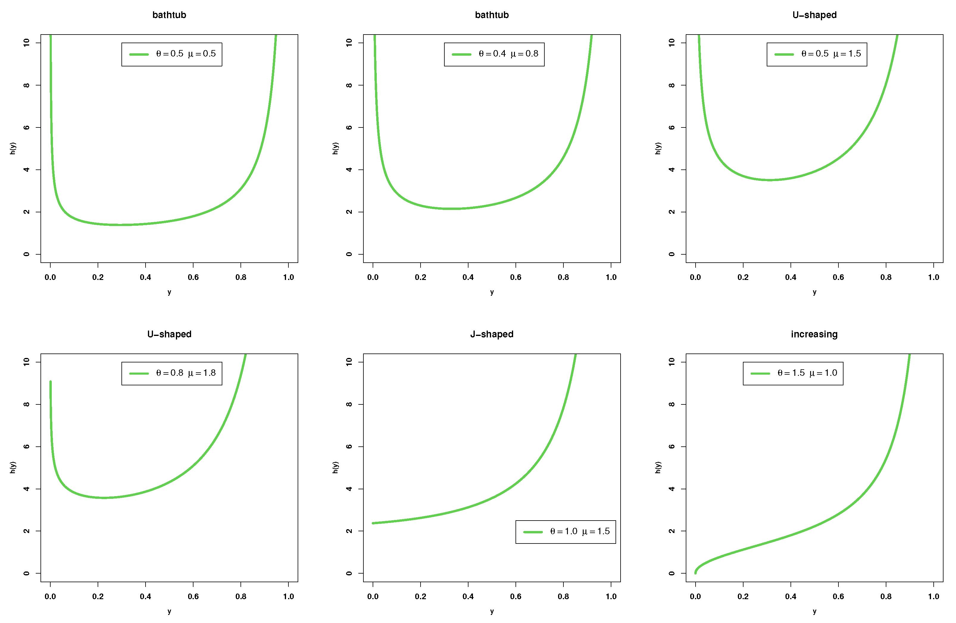
  • The curves of the pdf for the KMKu model are similar to the Ku model, and it can be asymmetric, such as (i) bathtub when  θ μ < 1 , (ii) decreasing when  θ 1 μ > 1 , (iii) increasing when  θ > 1 μ < 1 , (iv) unimodal when  θ > 1 , μ 1 .
  • The KMKu model has a closed form for the quantile function, making it simple to generate random numbers from the KMKu proposed model.
  • Several general statistical features of the KMku model were investigated.
  • The maximum likelihood estimation technique was employed to calculate the parameters of the KMKu model, employing simple and ranked set sampling.
  • The KMKu model gives more fit than the Ku model and numerous other well-known models for modeling real-world data sets in different fields, and we recommended that in the application section.
This paper is organized as follows. In Section 2, the construction of the KMKu model is provided by combining the Ku model and the KM transformation. In Section 3, we derive and investigate some important expansions, which we use to calculate the statistical properties of the KMKu model. In Section 4, some general statistical features of the KMKu model are derived. In Section 5, some different measures of entropy are computed. In Section 6, ranked set sampling is discussed. In Section 7, estimations of the unknown parameters using the maximum likelihood methodology under simple and ranked set sampling are studied. In Section 8, simulation outcomes are discussed. In Section 9, the importance and flexibility of the KMKu model are proved by employing three real data sets. Finally, the paper ended with concluding remarks.

2. The Construction of The Suggested Model

In this section, we create a new flexible statistical model defined as the Kavya–Manoharan transformation Kumaraswamy (KMKu) model by introducing (1) into (3) to obtain
F C D F F ( y ; θ , μ ) = e e 1 1 e 1 e 1 y θ μ ; 0 < y < 1 , θ , μ > 0 ,
and the corresponding pdf is
f ( y ; θ , μ ) = 1 e 1 θ μ y θ 1 1 y θ μ 1 e 1 y θ μ ; 0 < y < 1 , θ , μ > 0 .
The survival function, hrf and reversed hrf for the KMKu model are
R ( y ; θ , μ ) = 1 F ( y ; θ , μ ) = 1 e e 1 1 e 1 e 1 y θ μ ; 0 < y < 1 , θ , μ > 0 ,
h ( y ; θ , μ ) = f ( y ; θ , μ ) R ( y ; θ , μ ) = θ μ y θ 1 1 y θ μ 1 1 e 1 y θ μ ,
and
τ ( y ; θ , μ ) = f ( y ; θ , μ ) F ( y ; θ , μ ) = θ μ y θ 1 1 y θ μ 1 e 1 1 y θ μ 1 .
The cumulative hrf is provided via
H ( y ; θ , μ ) = ln 1 e e 1 1 e 1 e 1 y θ μ .
The inverse of the cdf was used to generate random samples from the newly suggested model, and it has the next equation
y u = 1 1 + ln 1 u 1 e 1 1 μ 1 θ .
Figure 1 shows the forms of the KMKu pdf (6) utilizing distinct parameter combinations. According to the values of the parameter, the pdf of the KMKu model is asymmetric, and it has one of these forms: (i) bathtub when  θ μ < 1 , (ii) decreasing when  θ 1 μ > 1 , (iii) increasing when  θ > 1 μ < 1 , (iv) unimodal when  θ > 1 , μ 1 .
Figure 2 demonstrates a graphical representation of the hrf of the KMKu model utilizing distinct parameter combinations. According to the values of the parameter, the hrf of the KMKu model can be bathtub, U-shaped and increasing.

3. Useful Expansions

In this section, the expansions of the  f ( y ; θ , μ ) f ( y ; θ , μ ) λ  and  F ( y ; θ , μ ) h  for the KMKu model are derived to make the computation of the statistical features easy because we can write the pdf and cdf of the KMKu model as a linear combination of the Ku model. First, we can rewrite Equation (6) as
f ( y ; θ , μ ) = θ μ e e 1 y θ 1 1 y θ μ 1 e 1 1 y θ μ ,
Using the exponential expansion  e β y = i = 0 ( 1 ) i β i y i i !  to Equation (8), we obtain,
f ( y ; θ , μ ) = θ μ e e 1 y θ 1 i = 0 1 i i ! 1 y θ μ 1 1 1 y θ i .
Using the binomial expansion
( 1 y ) β 1 = j = 0 ( 1 ) j β 1 j y j , y < 1 ,
by inserting Equation (10) in Equation (9), we obtain
f ( y ; θ , μ ) = y θ 1 i , j = 0 ς i , j 1 y θ μ + j 1 ,
where  ς i , j = θ μ e e 1 1 i + j i ! i j .
To obtain the expansion of  f ( y ; θ , μ ) λ , then
f ( y ; θ , μ ) λ = θ μ e e 1 λ y λ ( θ 1 ) 1 y θ λ ( μ 1 ) e λ 1 1 y θ μ ,
by applying the exponential expansion to the above equation, we obtain,
f ( y ; θ , μ ) λ = θ μ e e 1 λ y λ ( θ 1 ) i = 0 1 i λ i i 1 y θ λ ( μ 1 ) 1 1 y θ μ i ,
by applying the binomial expansion (10) in Equation (12), we obtain
f ( y ; θ , μ ) λ = y λ ( θ 1 ) i , j = 0 ϖ i , j 1 y θ λ ( μ 1 ) + j ,
where  ϖ i , j = θ μ e e 1 λ 1 i + j λ i i i j . To obtain the expansion of  F ( y ; θ , μ ) h , then
F ( y ; θ , μ ) h = e e 1 h 1 e 1 1 y θ μ h ,
by employing the binomial expansion  ( 1 y ) β 1 = k = 0 β 1 ( 1 ) k β 1 k y k , to the above equation, we obtain
F ( y ; θ , μ ) h = e e 1 h k = 0 h ( 1 ) k h k e k 1 1 y θ μ ,
again by employing the exponential expansion to the above equation, we obtain
F ( y ; θ , μ ) h = e e 1 h k = 0 h m = 0 ( 1 ) k + m k m m ! h k 1 1 y θ μ m ,
again by using the binomial expansion (10) to the above equation, we obtain
F ( y ; θ , μ ) h = k = 0 h m , s = 0 Ω k , m , s 1 y θ μ s ,
where  Ω k , m , s = e e 1 h ( 1 ) k + m + s k m m ! h k m s .

4. General Statistical Properties

The section discusses various essential characteristics of the KMku model, such as the quantile function (qf), raw and incomplete moments, probability-weighted moments, and order statistics.

4.1. Quantile Function

Quantile function (qf) is an important measure and is used to generate a random variate. Let  Y K M K u ( θ , μ )  for  Y > 0  and  θ , μ > 0 , then its qf, say Q(u), is given by in Equation (15)
Q u = 1 1 + ln 1 u 1 e 1 1 μ 1 θ ,
where u is a uniform distribution. The median (M) of the KMKu model may be calculated by entering u = 0.5 in Equation (15) as
M = 1 1 + ln 1 0.5 1 e 1 1 μ 1 θ .

4.2. Moments and Incomplete Moments

The wth moment of Y can be computed by using the next formula
μ w = 0 1 y w f ( y ; θ , μ ) d y .
We acquire Equation (11) by entering it into Equation (16)
μ w = i , j = 0 ς i , j 0 1 y w + θ 1 1 y θ μ + j 1 d y ,
Let  v = y θ , then we can write the previous equation as
μ w = 1 θ i , j = 0 ς i , j 0 1 v w θ 1 v μ + j 1 d v ,
then, the wth moment of the KMKu model is provided via
μ w = 1 θ i , j = 0 ς i , j B w θ + 1 , μ + j ,
where  B ( . , . )  is the B function. By putting  w = 1 , 2 , 3 , 4  in (17), we obtain the first four moments for Y as
μ 1 = 1 θ i , j = 0 ς i , j B 1 θ + 1 , μ + j ,
μ 2 = 1 θ i , j = 0 ς i , j B w θ + 1 , μ + j ,
μ 3 = 1 θ i , j = 0 ς i , j B 3 θ + 1 , μ + j ,
and
μ 4 = 1 θ i , j = 0 1 i ! B 4 θ + 1 , μ + j .
The mean and variance (var) of the KMKu model are computed as
m e a n = 1 θ i , j = 0 ς i , j B 1 θ + 1 , μ + j ,
and
V a r ( y ) = 1 θ i , j = 0 ς i , j B 2 θ + 1 , μ ( i + 1 ) 1 θ i , j = 0 ς i , j B 1 θ + 1 , μ + j 2 .
The skewness ( γ 1 ), kurtosis ( γ 2 ) are  γ 1 = μ 3 2 μ 2 3  and  γ 2 = μ 4 μ 2 2  where  μ 2 = μ 2 μ 1 2 μ 3 = μ 3 3 μ 1 μ 2 + 2 μ 1 3  and  μ 4 = μ 4 4 μ 3 μ 1 + 6 μ 2 μ 1 2 3 μ 1 4 .
By using Equation (12), Table 1 shows some numerical values of the first four moments  μ 1 μ 2 μ 3 μ 4 , the var,  γ 1 γ 2  and coefficient of variation ( C V = v a r μ ).
The pth incomplete moments for the KMKu model can be computed as
η p ( t ) = i , j = 0 ς i , j 0 t y p + θ 1 1 y θ μ + j 1 d y .
Let  v = y θ , then the pth incomplete moments for the KMKu model are
η p ( t ) = 1 θ i , j = 0 ς i , j B t θ p θ + 1 , μ + j ,
where  B y ( . , . )  is the incomplete B function.

4.3. Probability Weighted Moments

The  ( n , h ) th probability weighted moments (PWMs) of Y following the KMKu model, symbolized as  τ n , h , are formally computed from the next formula
τ n , h = 0 1 y n f ( y ; θ , μ ) F y ; θ , μ h d y .
By inserting the two Equations (11) and (14) into (22), then we obtain
τ n , h = i , j = 0 k = 0 h m , s = 0 Ω k , m , s ς i , j 0 1 y n + θ 1 1 y θ μ ( s + 1 ) + j 1 d y .
Let  v = y θ , then the PWMs of the KMKu model are
τ n , h = 1 θ i , j = 0 k = 0 h m , s = 0 Ω k , m , s ς i , j B n θ + 1 , μ ( s + 1 ) + j .

4.4. Order Statistics

A sample of size n is taken from the KMKu model and, by the following definition, yielded the pdf of ith order statistics for the KMKu model
f i : n ( y ; θ , μ ) = 1 B ( i , n i + 1 ) f ( y ; θ , μ ) l = 0 n i ( 1 ) l n i l F ( y ; θ , μ ) i + l 1 .
By employing (11) and (14) into (24) and replacing h with  i + l 1 , then
f i : n ( y ; θ , μ ) = l = 0 n i i , j = 0 k = 0 i + l 1 m , s = 0 Ω l , i , j , k , m , s y θ 1 1 y θ μ ( s + 1 ) + j 1 ,
where  Ω l , i , j , k , m , s = ( 1 ) l B i , n i + 1 n i l Ω k , m , s ς i , j .  For more information see [20,21].

5. Different Types of Entropy

Entropy measurements are significant in investigations of dependability and risk. It has been employed in a variety of biological, medicinal, and physical applications.

5.1. Rényi Entropy

The essential shape of the distribution is measured using Rényi entropy (RE) [22], and it is provided by
R λ = 1 1 λ log 0 1 ( f ( y ; θ , μ ) ) λ d y , λ > 0 , λ 1 .
By employing (13) into (25), then
R λ = 1 1 λ log i , j = 0 ϖ i , j 0 1 y λ ( θ 1 ) 1 y θ λ μ 1 + j d y .
Let  v = y θ , then
R λ = 1 1 λ log 1 θ i , j = 0 ϖ i , j 0 1 v λ λ + 1 θ 1 1 v λ μ 1 + j d v .
The RE of the KMKu model is
R λ = 1 1 λ log 1 θ i , j = 0 ϖ i , j B λ λ + 1 θ , λ μ 1 + j + 1 .

5.2. Havrda and Charvat Entropy

The Havrda and Charvat entropy (HCE) [23] measure is provided via
H C λ = 1 2 1 λ 1 0 1 ( f ( y ; θ , μ ) ) λ d y 1 λ 1 , λ > 0 , λ 1 .
By employing (13) into (26), then
H C λ = 1 2 1 λ 1 1 θ i , j = 0 ϖ i , j 0 1 y λ ( θ 1 ) 1 y θ λ μ 1 + j d y 1 λ 1 .
After some computational, then the HCE of the KMKu model is
H C λ = 1 2 1 λ 1 1 θ i , j = 0 ϖ i , j B λ λ + 1 θ , λ μ 1 + j + 1 .

5.3. Tsallis Entropy

The Tsallis entropy (TE) [24] measure is provided by
T λ = 1 λ 1 1 0 1 ( f ( y ; θ , μ ) ) λ d y , λ > 0 , λ 1 .
By employing (13) into (27), then
T λ = 1 λ 1 1 1 θ i , j = 0 ϖ i , j 0 1 y λ ( θ 1 ) 1 y θ λ μ 1 + j d y .
After some computational, then the TE of the KMKu model is
T λ = 1 λ 1 1 1 θ i , j = 0 ϖ i , j B λ λ + 1 θ , λ μ 1 + j + 1 .

5.4. Arimoto Entropy

The Arimoto entropy (AE) [25] measure is provided by
A λ = λ 1 λ 0 1 ( f ( y ; θ , μ ) ) λ d y 1 λ 1 , λ > 0 , λ 1 .
By employing (13) into (28), then
A λ = λ 1 λ 1 θ i , j = 0 ϖ i , j 0 1 y λ ( θ 1 ) 1 y θ λ μ 1 + j d y 1 λ 1 .
After some computational, then the AE of the KMKu model is
A λ = λ 1 λ 1 θ i , j = 0 ϖ i , j B λ λ + 1 θ , λ μ 1 + j + 1 1 λ 1 .
Table 2 shows some numerical values of the different types of entropy.

6. Sampling Techniques

The most popular sampling methods are simple random sampling (SRS) and ranked set sampling (RSS). SRS is the most common method of data collection. In many applications (such as fisheries and medical research), where actual measurement of the variable of interest would be either time-consuming or expensive, ranking a number of sampling units without actually measuring them can be performed reasonably simply and affordably. To obtain more representative samples from the underlying population and boost the effectiveness of the statistical inference under these circumstances, rank-based sampling strategies may be used. McIntyre’s initial suggestion of RSS is cited in references [26,27]. Numerous studies have shown that RSS-based statistical procedures are superior to their SRS scheme analogs, either numerically or theoretically. The initial ranking of n samples of size n for the one-cycle RSS looks like this:
1 . Y 1 ( 1 : n ) s ̲ Y 1 ( 2 : n ) s , Y 1 ( n : n ) s Z 1 s = Y 1 ( 1 : n ) s 2 . Y 2 ( 1 : n ) s Y 2 ( 2 : n ) s ̲ Y 2 ( n : n ) s Z 2 s = Y 2 ( 2 : n ) s n . Y n ( 1 : n ) s Y n ( 2 : n ) s Y n ( n : n ) s ̲ Z n s = Y n ( n : n ) s
where s cycles to produce a sample of size  N = n s , and  Y j ( i : n ) s  denotes the ith order statistic from the jth SRS of size N. The resulting sample is called a one-cycle RSS and has the size  n = N . It is represented by the symbol  Z ̲ = ( Z 11 , Z 21 , , Z n 1 ) Z i 1 . Under the premise of perfect judgement ranking,  Z i 1  has the same distribution as  Y i ( i : n ) s , the ith order statistic in a set of size n generated from the ith sample with pdf, see [28].
g ( i ) ( z ) = n ! ( i 1 ) ! ( n i ) ! [ F ( z ) ] i 1 [ 1 F ( z ) ] n i f ( z ) , < z < .
The cycle can be repeated s times until  N = s n  units are quantified.
Following that, several extensions to the original RSS were proposed. Assessing the performance of some ranked set of sampling designs using a hybrid approach has been discussed by [29]; RSS with the application of modified Kies exponential distribution has been obtained by [30]; some properties and estimations under RSS of the generalized Bilal distribution has been introduced by [31]; an estimation of the exponential parameters of the Pareto distribution under ranked- and double-RSS designs has been obtained [32]; and Bayesian estimation using an MCMC method of system reliability for inverted Topp–Leone distribution based on RSS has been introduced by [33]. Contrarily, median RSS and MRSS [34] only consider the units that rank as the median for each set. While paired RSS [35] is a less expensive alternative that ranks fewer units, double RSS [36] is a more effective but also more expensive version of RSS that rates a higher number of sets in two ordering stages. For other probability distributions, see the recently proposed sampling technique in [37,38,39,40,41,42,43,44].

7. Maximum Likelihood Estimation

In this section, we obtain the parameter estimator of  θ  and  μ  based on SRS and RSS.

7.1. MLE Based on SRS

Here, using SRS, we first need to obtain the MLE of  θ  and  μ . Let  Y i i = ( 1 , , N )  be an independent SRS drawn from  Y K M K u ( θ , μ ) . The likelihood function based on SRS is:
L ( θ , μ ) = i = 1 N f Y ( y i ) = 1 e 1 N θ N μ N e i = 1 N 1 y i θ μ i = 1 N y i θ 1 1 y i θ μ 1 .
The ln-likelihood function of the observed samples is
( θ , μ ) = N ln 1 e 1 + ln ( θ ) + ln ( μ ) + i = 1 N 1 y i θ μ + ( θ 1 ) i = 1 N ln ( y i ) + ( μ 1 ) i = 1 N ln 1 y i θ .
The partial derivatives of (31) with respect to  θ  and  μ  to obtain the ln-likelihood equations are
( θ , μ ) θ = N θ μ i = 1 N y i θ ln ( y i ) 1 y i θ μ 1 + i = 1 N ln ( y i ) ( μ 1 ) i = 1 N y i θ ln ( y i ) 1 y i θ ,
( θ , μ ) μ = N μ + i = 1 N 1 y i θ μ ln 1 y i θ + i = 1 N ln ( 1 y i θ ) .
Two non-linear systems of equations that are differentiating (32) and (33) with respect to  θ  and  μ , respectively, and equating each solution to zero must be solved concurrently in order to create MLE for SRS. One can use the R statistical programming language software to compute the desired MLEs  θ  and  μ  for any given data set by utilizing the “optim” function of the “stats” package, which employs the Nelder–Mead (NM) approach of maximization in the maximum likelihood computations.

7.2. MLE Based on RSS

Let  Y i ( i : n s ) , i = 1 , , n s , s = 1 , , p  be an s-cycle of RSS from the KMKu( θ , μ ). We denote  Y i ( i : n ) s  by  Y i s  to simplify the notation. The function based on RSS by using Equation (29) is:
g i : n s ( z i s ; θ , μ ) = C i : n s F ( z i s ; θ , μ ) i 1 1 F ( z i s ; θ , μ ) n s i f ( z i s ; θ , μ ) ,
where  C i : n s = n s ! ( i 1 ) ! ( n s i ) ! . In view of (29), the likelihood function can be written as
L ( θ , λ ; z i s ) = s = 1 p i = 1 n s g i ( z i s ; θ , μ ) = s = 1 p i = 1 n s C i : n s e e 1 i 1 1 e 1 e 1 z i s θ μ i 1 1 e e 1 1 e 1 e 1 z i s θ μ n s i × s = 1 p i = 1 n s 1 e 1 θ μ z i s θ 1 1 z i s θ μ 1 e 1 z i s θ μ .
where  N = s = 1 p n s  In this setting, the log-likelihood function of the KMKu distribution is given by
( θ , μ ; z i s ) = s = 1 p i = 1 n s ln ( C i : n s ) + s = 1 p i = 1 n s ( i 1 ) ln e e 1 + s = 1 p i = 1 n s ( i 1 ) ln 1 e 1 e 1 z i s θ μ + s = 1 p i = 1 n s ( n s i ) ln 1 e e 1 1 e 1 e 1 z i s θ μ + N ln 1 e 1 + l o g ( θ ) + ln ( μ ) + ( θ 1 ) s = 1 p i = 1 n s ln ( z i s ) + ( μ 1 ) s = 1 p i = 1 n s ln 1 z i s θ + s = 1 p i = 1 n s 1 z i s θ μ
The partial derivatives of  ( θ , μ ; z i s )  associated with unknown parameters can be expressed as
( θ , μ ; z i s ) θ = μ s = 1 p i = 1 n s ( i 1 ) ln ( z i s ) z i s θ 1 z i s θ μ 1 e 1 e 1 z i s θ μ 1 e 1 e 1 z i s θ μ + N θ + s = 1 p i = 1 n s ln ( z i s ) e e 1 μ s = 1 p i = 1 n s ( n s i ) ln ( z i s ) z i s θ 1 z i s θ μ 1 e 1 e 1 z i s θ μ 1 e e 1 1 e 1 e 1 z i s θ μ ( μ 1 ) s = 1 p i = 1 n s ln ( z i s ) z i s θ 1 z i s θ μ s = 1 p i = 1 n s ln ( z i s ) z i s θ 1 z i s θ μ 1
and
l ( θ , μ ; x ( i i ) j ) μ = e 1 s = 1 p i = 1 n s ( i 1 ) ln 1 z i s θ 1 z i s θ μ e 1 z i s θ μ 1 e 1 e 1 z i s θ μ + N μ + s = 1 p i = 1 n s ln 1 z i s θ + 1 e 1 s = 1 p i = 1 n s ( n s i ) ln 1 z i s θ 1 z i s θ μ e 1 z i s θ μ 1 e e 1 1 e 1 e 1 z i s θ μ + s = 1 p i = 1 n s ln 1 z i s θ 1 z i s θ μ .
By numerically solving the nonlinear equations  ( θ , μ ; z i s ) θ = 0  and  ( θ , μ ; z i s ) μ = 0  with respect to  θ  and  μ , the MLEs can be obtained.

7.3. Asymptotic Confidence Interval

The Hessian matrix by the “optim” function yields the Fisher information matrix I of parameters  θ  and  μ , which are the negative expectation of the last-second derivative of the log-likelihood function and  θ  and  μ , respectively. The inverse Fisher information matrix describes the variance-covariance matrix. The asymptotic distribution of the MLE  ( θ ^ , μ ^ )  is also given as  n  increases:
θ ^ μ ^ N θ μ , V ^ 11 V ^ 12 V ^ 21 V ^ 22
.
By inverting the Hessian matrix, the estimates  θ ^  and  μ ^  of theasymptotic variance-covariance matrix V are produced. The following equations provide two-sided  100 ( 1 α ) %  confidence intervals (CI) for  θ  and  μ :
L o w e r ( θ ) = θ ^ Z α 2 V ^ 11 , U p p e r ( θ ) = θ ^ + Z α 2 V ^ 11 ,
and
L o w e r ( μ ) = μ ^ Z α 2 V ^ 22 , U p p e r ( μ ) = μ ^ + Z α 2 V ^ 22 ,
respectively, where  Z α 2  is the  α 2  percentile of the standard normal distribution.

8. Simulation

Some calculations are made in accordance with Monte Carlo simulation experiments using R packages with various combinations of sample sizes n and cycle size s as part of our rigorous effort to assess the effectiveness of the inference methods suggested in this paper. We generate a KMKu sample with the parameters ( θ , μ ): (0.2, 0.75), (0.2, 1.5), (0.2, 3), (0.5, 0.75), (0.5, 1.5), and (0.5, 3). It has been determined how well the resulting  θ , and  μ  estimators perform in terms of their bias, corresponding mean squared error (MSE), relative efficiencies (REs) and coverage probability (CP) as follows:
B i a s ( θ ) = 1 N I i = 1 N I θ ^ θ , M S E ( μ ) = 1 N I i = 1 N I μ ^ μ ,
M S E ( θ ) = 1 N I i = 1 N I θ ^ θ 2 , M S E ( μ ) = 1 N I i = 1 N I μ ^ μ 2 ,
R E 1 ( θ ) = M S E S R S ( θ ) M S E R S S s = 1 ( θ ) , R E 2 ( θ ) = M S E S R S ( θ ) M S E R S S s = 3 ( θ ) , R E 3 ( θ ) = M S E R S S s = 1 ( θ ) M S E R S S s = 3 ( θ ) ,
R E 1 ( μ ) = M S E S R S ( μ ) M S E R S S s = 1 ( μ ) , R E 2 ( μ ) = M S E S R S ( μ ) M S E R S S s = 3 ( μ ) , R E 3 ( μ ) = M S E R S S s = 1 ( μ ) M S E R S S s = 3 ( μ ) .
C P ( μ ) = M e a n 1 if L o w e r ( μ ) μ ^ U p p e r ( μ ) 0 otherwise ,
and
C P ( θ ) = M e a n 1 if L o w e r ( θ ) θ ^ U p p e r ( θ ) 0 otherwise .
Using a Monte Carlo simulation in R software (we used function “optim” in R-package “stats”) with  N = 10,000 repeats for various set sizes, the number of cycles, and chosen parameter values, the performance of the estimations is compared. To generate a sample of RSS, we used function “rss” in R-package “RSSampling”, which the “rss” function samples from a target population by using a ranked set sampling method.
Table 3 and Table 4 present the results of the simulation investigation. As sample size increases, bias and MSE decrease. We see that bias and MSE values based on RSS are always less than those based on SRS. Additionally, as sample sizes are increased for all parameters, the MSE values based on the SRS and RSS techniques become lower. Figure 3 shows the MSE values of parameters based on SRS with different sample sizes and different parameter values, and this indicates that the MSE decreases when sample size increases. 
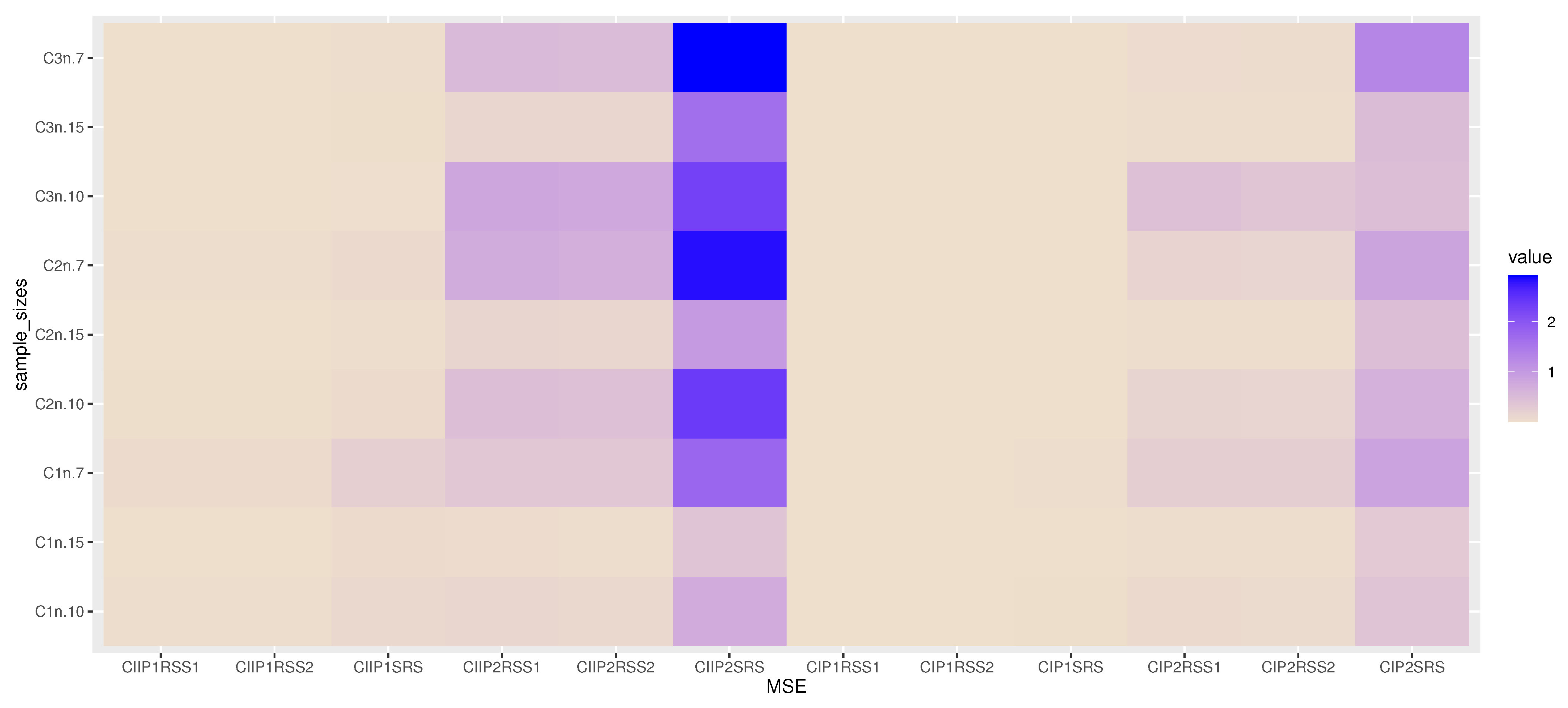
Figure 4 shows the heat map for MSE values of parameters based on RSS with different fixed values of sample sizes and parameters, and  μ  increases, the MSE for  θ  decreases, while the MSE for  μ  increases. In Figure 4, the X label is MSE for different methods of each parameter: CIP1SRS is MSE of SRS for  θ  when  θ = 0.2 , CIP2SRS is MSE of SRS for  μ  when  θ = 0.2 , etc., while the Y label is MSE with different sample sizes, where C1n7 is MSE when  μ = 0.75  and n = 7, C2n7 is MSE when  μ = 1.5  and n = 7, etc. The results of the simulation show that the RSS scheme performs better than the SRS method. We can also infer that the RSS technique is more effective than the SRS scheme for estimating the unknown parameters of the KMKu distribution. The results of RSS in simulation tables show that the RSS with a greater cycle, s = 3, is superior to the RSS with a single cycle.

9. Application

This section compares the KMKu distribution with well-known unit distributions in the literature by analyzing three data sets, one of which is connected to coronavirus data and the others to burr measurements on iron sheets. These models for comparison are (together with their pdfs for  ( 0 y 1 ) ): unit Weibull (UW), which was discussed by [45], Ku, B; Marshall–Olkin Ku (MOKu), which introduced by [8]; unit-Gompertz (UG), which was obtained by [46]; Marshall–Olkin-extended Topp–Leone (MOTL), which was discussed by [47]; and unit-exponentiated half logistic (UEHL), which was introduced by [48].
For all statistical models, we also calculate the goodness-of-fit statistics for the estimated different measures such as “Akaike Information Criteria (AIC), corrected AIC (CAIC), Bayesian information criterion (BIC), Hannan–Quinn information criterion (HQIC), Kolmogorov–Smirnov distance (KSS), p-value (PVKS), Cramer-von-Mises (WS), and Anderson–Darling (AS)”. The model with the smaller AIC, CAIC, BIC, HQIC, KSS, WS, and AS statistics and the higher PVKS of the goodness-of-fit statistics is typically considered to be the best one. It should be noted that the MLE approach was used to achieve all results.
We used SRS and RSS techniques with various set sizes and cycle counts to observe random samples of various sizes for analysis. We then computed MLEs of the parameters for the observed SRS and RSS with various cycle counts, and we compared the performance of the estimates.
Firstly: The COVID-19 data in question are mortality rates from the United Kingdom and span 82 days, from May 1 to July 16, 2021, as follows: 0.0023, 0.0023, 0.0023, 0.0046, 0.0065, 0.0067, 0.0069, 0.0069, 0.0091, 0.0093, 0.0093, 0.0093, 0.0111, 0.0115, 0.0116, 0.0116, 0.0119, 0.0133, 0.0136, 0.0138, 0.0138, 0.0159, 0.0161, 0.0162, 0.0162, 0.0162, 0.0163, 0.0180, 0.0187, 0.0202, 0.0207, 0.0208, 0.0225, 0.0230, 0.0230, 0.0239, 0.0245, 0.0251, 0.0255, 0.0255, 0.0271, 0.0275, 0.0295, 0.0297, 0.0300, 0.0302, 0.0312, 0.0314, 0.0326, 0.0346, 0.0349, 0.0350, 0.0355, 0.0379, 0.0384, 0.0394, 0.0394, 0.0412, 0.0419, 0.0425, 0.0461, 0.0464, 0.0468, 0.0471, 0.0495, 0.0501, 0.0521, 0.0571, 0.0588, 0.0597, 0.0628, 0.0679, 0.0685, 0.0715, 0.0766, 0.0780, 0.0942, 0.0960, 0.0988, 0.1223, 0.1343, 0.1781. This data have been cited in https://covid19.who.int/ (accessed on 1 February 2023). Table 5 discusses the MLE for different models with different measures of goodness-of-fit for COVID-19 data of the United Kingdom. Figure 5 shows estimated cdf with empirical cdf, estimated pdf with histogram probability of COVID-19 data of the United Kingdom and a P-P plot for KMKu. 
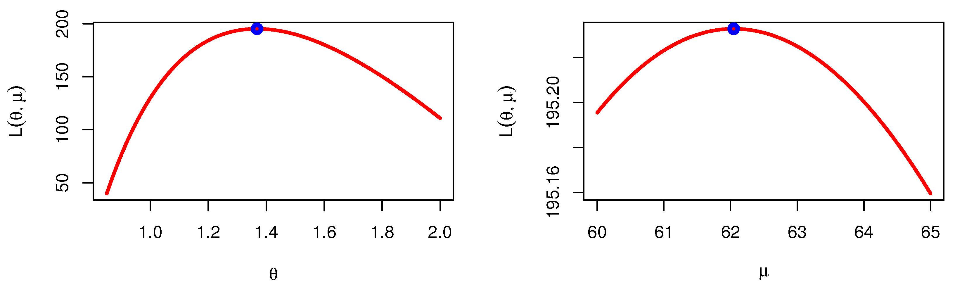
Figure 6 was obtained to check whether the estimators are maximum or not for parameters of the KMKu distribution based on COVID-19 data of the United Kingdom.
In the first set of data, we obtained the RSS data for when N = 50 with one cycle, as shown in Table 6, and we obtained the RSS data for when the size was n = 5, and the cycle was  s = 10 , as shown in Table 7. According to these data, the MLE based on SRS and RSS with the different cycles for COVID-19 data of the United Kingdom when n = 50 is shown in Table 8.
The second data set relates to the newly discovered coronavirus epidemic in Turkey. This dataset has been cited in https://covid19.who.int/ (accessed on 1 February 2023). A total of 25 observations make up this data set, which covers the period from 27 March to 20 April and was calculated as the daily ratio of recoveries to confirm cases in Turkey. This indicates the daily proportion of people making a full recovery in all circumstances. The information was provided in data set II as follows: 0.0074 0.0095 0.0113 0.0150 0.0180 0.0212 0.0229 0.0231 0.0328 0.0385 0.0439 0.0464 0.0483 0.0507 0.0515 0.0568 0.0605 0.0648 0.0737 0.0818 0.0955 0.1099 0.1270 0.1388 0.1476. Table 9 presents the MLE for different models with different measures of goodness-of-fit for the COVID-19 data of Turkey. Figure 7 shows the estimated cdf with empirical cdf, the estimated pdf with histogram probability of COVID-19 data of Turkey, and the P–P plot for KMKu. 
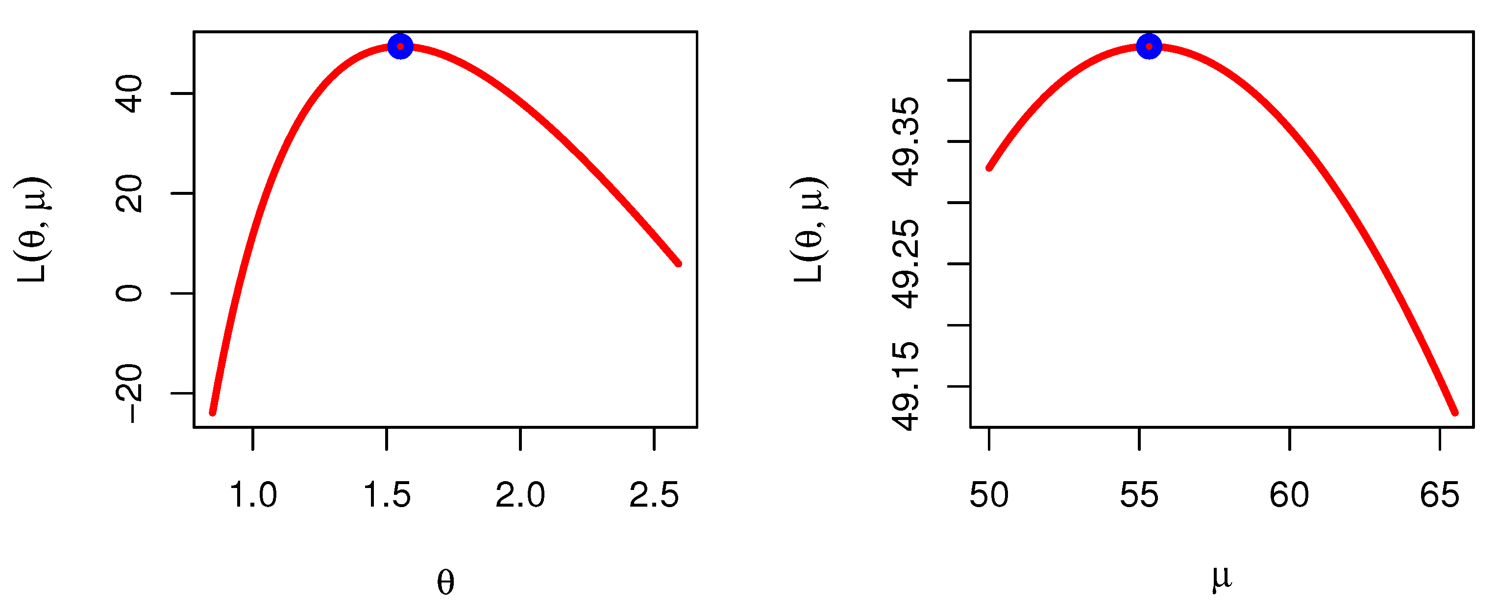
Figure 8 was produced to check whether the estimators are maximums or not for the parameters of KMKu distribution based on COVID-19 data of Turkey.
In the second data set, we obtained the RSS data for when N = 15 with one cycle, as shown in Table 6, and we obtained the RSS data for when the size is n = 5 and the cycle is  s = 3 , as shown in Table 7. According to these data, the MLE based on SRS and RSS with the different cycles for COVID-19 data of Turkey when n = 15 is shown in Table 10.
The third data set included 30 measurements of polyester fibers’ tensile strength, which has been discussed by [46]. The information is provided in data set III as follows: “0.023, 0.032, 0.054, 0.069, 0.081, 0.094, 0.105, 0.127, 0.148, 0.169, 0.188, 0.216, 0.255, 0.277, 0.311, 0.361, 0.376, 0.395, 0.432, 0.463, 0.481, 0.519, 0.529, 0.567, 0.642, 0.674, 0.752, 0.823, 0.887, 0.926”. Table 11 discusses MLE for different models with different measures of goodness-of-fit for data on the strength of polyester fibers. Figure 9 shows estimates cdf with empirical cdf, the pdf with histogram probability of data on the strength of polyester fibers, and the P–P plot for KMKu. Figure 10 was produced to check whether the estimators are maximums or not for parameters of KMKu distribution based on data on the strength of polyester fibers.
In the third data set, we obtained the RSS data for when N = 15 with one cycle, as shown in Table 6, and we obtained the RSS data for when the size is n = 5 and the cycle is  s = 3 , as shown in Table 7. By these data, the MLE based on SRS and RSS with the different cycles for data on the strength of polyester fibers when n = 15 is shown in Table 12.
By delivering the lowest AIC, BIC, CAIC, HQIC WS, and AS values in Table 5, Table 9 and Table 11, the model fitted to KMKu is clearly outperforming other competitive models, such as UW, UG, Ku, B, UEHL, MOETL, and MOKu. This indicates that KMKu-based models provide more accurate and fitting information about these three real data sets. Figure 6, Figure 8 and Figure 10 show the parameters of the KMKu model have a maximum log-likelihood with the other parameters fixed. Table 8, Table 10 and Table 12 make it evident that the model fitted using the RSS design is outperforming the other competing models by offering the lowest SE, indicating that RSS-based models are more accurate at representing the real model utilized in these numerical examples.

10. Concluding Remarks

In this article, we proposed and studied a new extension of the Ku model, which is called the KMKu model. The shape forms of the pdf for the new KMKu model for various values of parameters are is similar to the Ku model in that it is asymmetric. Some general statistical and computational features of the KMKu model, such as the qf, raw and incomplete moments, probability-weighted moments, and order statistics, were calculated. Four different measures of entropy were discussed. The maximum likelihood approach was employed to estimate the parameters for the KMKu model under simple and ranked set sampling. A simulation experiment is conducted to show that ranked set sampling is more efficient than simple random sampling. The KMKu has more flexibility than the Ku model and other well-known models, such as the UW model, Ku model, B model, MOKu model, UG model, MOTL model, and UEHL model. The KMKu model gives the best fit for the three real-world data sets.

Author Contributions

Conceptualization, I.E.; Methodology, N.A., M.S., A.S.A.-M., M.E., E.M.A. and I.E.; Software, N.A., M.S., A.S.A.-M., M.E., E.M.A. and I.E.; Formal analysis, N.A., M.S., A.S.A.-M., M.E., E.M.A. and I.E.; Data curation, N.A., M.S., A.S.A.-M., M.E., E.M.A. and I.E.; Writing—original draft, N.A., M.S., A.S.A.-M., M.E., E.M.A. and I.E.; Supervision, N.A., M.S., A.S.A.-M., M.E., E.M.A. and I.E. All authors have read and agreed to the published version of the manuscript.

Funding

The authors extend their appreciation to the Deanship of Scientific Research at Imam Mohammad Ibn Saud Islamic University for funding this work through Research Grant No. (221412039).

Data Availability Statement

Data sets are available in the application section.

Acknowledgments

The authors extend their appreciation to the Deanship of Scientific Research, Imam Mohammad Ibn Saud Islamic University (IMSIU), Saudi Arabia, for funding this research work through Grant No. (221412039).

Conflicts of Interest

The authors declare no conflict of interest.

References

  1. Gupta, P.L.; Gupta, R.C. The monotonicity of the reliability measures of the beta distribution. Appl. Math. Lett. 2000, 13, 5–9. [Google Scholar] [CrossRef] [Green Version]
  2. Ghitany, M.E. The monotonicity of the reliability measures of the beta distribution. Appl. Math. Lett. 2004, 17, 1277–1283. [Google Scholar] [CrossRef]
  3. Kumaraswamy, P. A generalized probability density function for double-bounded random processes. J. Hydrol. 1980, 46, 79–88. [Google Scholar] [CrossRef]
  4. Lemonte, A.J.; Souzaa, W.B.; Cordeiro, G.M. The exponentiated Kumaraswamy distribution and its log-transform. Braz. J. Probab. Stat. 2013, 27, 31–53. [Google Scholar] [CrossRef]
  5. El-Sherpieny, E.-S.; Ahmed, M.A. On the Kumaraswamy Kumaraswamy distribution. Int. J. Basic Appl. Sci. 2014, 3, 372–381. [Google Scholar] [CrossRef] [Green Version]
  6. Khan, M.S.; King, R.; Hudson, I.L. Transmuted Kumaraswamy distribution. Stat. Transit. New Ser. 2016, 17, 183–210. [Google Scholar] [CrossRef] [Green Version]
  7. Sharma, D.; Chakrabarty, T.K. On size biased Kumaraswamy distribution. Stat. Optim. Inf. Comput. 2016, 4, 252–264. [Google Scholar] [CrossRef] [Green Version]
  8. George, R.; Thobias, S. Marshall-Olkin Kumaraswamy distribution. Int. Math. Forum 2017, 12, 47–69. [Google Scholar] [CrossRef]
  9. Elgarhy, M.; ul Haq, M.A.; ul Ain, Q. Exponentiated Generalized Kumaraswamy Distribution with Applications. Ann. Data. Sci. 2018, 5, 273–292. [Google Scholar] [CrossRef]
  10. Bantan, R.A.R.; Chesneau, C.; Jamal, F.; Elgarhy, M.; Almutiry, W.; Alahmadi, A.A. Study of a Modified Kumaraswamy Distribution. Mathematics 2021, 9, 2836. [Google Scholar] [CrossRef]
  11. ZeinEldin, R.A.; Haq, M.A.; Hashmi, S.; Elsehety, M.; Elgarhy, M. Type II Half Logistic Kumaraswamy Distribution with Applications. J. Funct. Spaces 2020, 2020, 1343596. [Google Scholar] [CrossRef]
  12. Ulubekova, F.; Ozel, G. Alpha power-kumaraswamy distribution with an application on survival times of cancer patients. J. Comput. Sci. Res. 2020, 2, 30–36. [Google Scholar] [CrossRef]
  13. Ghosh, I. Bivariate and multivariate weighted Kumaraswamy distributions: Theory and applications. J. Stat. Theory Appl. 2019, 18, 198–211. [Google Scholar] [CrossRef] [Green Version]
  14. Alyami, S.A.; Babu, M.G.; Elbatal, I.; Alotaibi, N.; Elgarhy, M. Type II Half-Logistic Odd Fréchet Class of Distributions: Statistical Theory and Applications. Symmetry 2022, 14, 1222. [Google Scholar] [CrossRef]
  15. Elbatal, I.; Alotaibi, N.; Almetwally, E.M.; Alyami, S.A.; Elgarhy, M. On Odd Perks-G Class of Distributions: Properties, Regression Model, Discretization, Bayesian and Non-Bayesian Estimation, and Applications. Symmetry 2022, 14, 883. [Google Scholar] [CrossRef]
  16. Bantan, R.A.R.; Jamal, F.; Chesneau, C.; Elgarhy, M. Type II Power Topp-Leone Generated Family of Distributions with Statistical Inference and Applications. Symmetry 2020, 12, 75. [Google Scholar] [CrossRef] [Green Version]
  17. Hamdy, A.; Almetwally, E.M. Bayesian and Non-Bayesian Inference for The Generalized Power Akshaya Distribution with Application in Medical. Comput. J. Math. Stat. Sci. 2023, 2, 31–51. [Google Scholar] [CrossRef]
  18. Souza, L.; de Oliveira, W.R.; de Brito, C.C.R.; Chesneau, C.; Fernandes, R.; Ferreira, T.A.E. Sec-G Class of Distributions: Properties and Applications. Symmetry 2022, 14, 299. [Google Scholar] [CrossRef]
  19. Kavya, P.; Manoharan, M. Some parsimonious models for lifetimes and applications. J. Statist. Comput. Simul. 2021, 91, 3693–3708. [Google Scholar] [CrossRef]
  20. Mustafa, G.; Ijaz, M.; Jamal, F. Order Statistics of Inverse Pareto Distribution. Comput. J. Math. Stat. Sci. 2022, 1, 51–62. [Google Scholar] [CrossRef]
  21. Sobhi, A.L.; Mashail, M. Moments of Dual Generalized Order Statistics and Characterization for Transmuted Exponential Model. Comput. J. Math. Stat. Sci. 2022, 1, 42–50. [Google Scholar] [CrossRef]
  22. Rényi, A. On measures of entropy and information. In Proceedings of the 4th Fourth Berkeley Symposium on Mathematical Statistics and Probability, Berkeley, CA, USA, 30 June–30 July 1960; pp. 547–561. [Google Scholar]
  23. Havrda, J.; Charvat, F. Quantification method of classification processes, Concept of Structural -Entropy. Kybernetika 1967, 3, 30–35. [Google Scholar]
  24. Tsallis, C. The role of constraints within generalized non-extensive statistics. Physica 1998, 261, 547–561. [Google Scholar]
  25. Arimoto, S. Information-theoretical considerations on estimation problems. Inf. Control. 1971, 19, 181–194. [Google Scholar] [CrossRef] [Green Version]
  26. McIntyre, G.A. A method for unbiased selective sampling, using ranked sets. Aust. J. Agric. Res. 1952, 3, 385–390. [Google Scholar] [CrossRef]
  27. Hassan, O.H.M.; Elbatal, I.; Al-Nefaie, A.H.; Elgarhy, M. On the Kavya-Manoharan-Burr X Model: Estimations under ranked set sampling and applications. Risk Financ. Manag. 2023, 16, 19. [Google Scholar] [CrossRef]
  28. Takahasi, K.; Wakimoto, K. On unbiased estimates of the population mean based on the sample stratified by means of ordering. Ann. Inst. Stat. Math. 1968, 20, 1–31. [Google Scholar] [CrossRef]
  29. Sabry, M.A.; Almetwally, E.M.; Almongy, H.M.; Ibrahim, G.M. Assessing the performance of some ranked set sampling designs using hybrid approach. Comput. Mater. Contin. 2021, 68, 3737–3753. [Google Scholar]
  30. Aljohani, H.M.; Almetwally, E.M.; Alghamdi, A.S.; Hafez, E.H. Ranked set sampling with application of modified kies exponential distribution. Alex. Eng. J. 2021, 60, 4041–4046. [Google Scholar] [CrossRef]
  31. Akhter, Z.; Almetwally, E.M.; Chesneau, C. On the Generalized Bilal Distribution: Some Properties and Estimation under Ranked Set Sampling. Axioms 2022, 11, 173. [Google Scholar] [CrossRef]
  32. Sabry, M.H.; Almetwally, E.M. Estimation of the exponential pareto distribution’s parameters under ranked and double ranked set sampling designs. Pak. J. Stat. Oper. Res. 2021, 17, 169–184. [Google Scholar] [CrossRef]
  33. Yousef, M.M.; Hassan, A.S.; Al-Nefaie, A.H.; Almetwally, E.M.; Almongy, H.M. Bayesian estimation using MCMC method of system reliability for inverted Topp–Leone distribution based on ranked set sampling. Mathematics 2022, 10, 3122. [Google Scholar] [CrossRef]
  34. Muttlak, H. Median ranked set sampling with concomitant variables and a comparison with ranked set sampling and regression estimators. Environmetrics 1998, 9, 255–267. [Google Scholar] [CrossRef]
  35. Hossain, S.; Muttlak, H. Paired ranked set sampling: A more efficient procedure. Environmetrics 1999, 10, 195–212. [Google Scholar] [CrossRef]
  36. Al-Saleh, M.F.; Al-Kadiri, M.A. Double-ranked set sampling. Stat. Probab. Lett. 2000, 48, 205–212. [Google Scholar] [CrossRef]
  37. Al-Omari, A.I.; Haq, A. Novel entropy estimators of a continuous random variable. Int. J. Model. Simul. Sci. Comput. 2019, 10, 195004. [Google Scholar] [CrossRef]
  38. Bouza-Herrera, C.N.; Al-Omari, A.I.F. Ranked Set Sampling: 65 Years Improving the Accuracy in Data Gathering; Academic Press: London, UK, 2018. [Google Scholar]
  39. Khan, Z.; Ismail, M.; Samawi, H. Mixture ranked set sampling for estimation of population mean and median. J. Stat. Comput. Simul. 2020, 90, 573–585. [Google Scholar] [CrossRef]
  40. Pedroso, V.C.; Taconeli, C.A.; Giolo, S.R. Estimation based on ranked set sampling for the twoparameter birnbaum–saunders distribution. J. Stat. Comput. Simul. 2021, 91, 316–333. [Google Scholar] [CrossRef]
  41. Qian, W.; Chen, W.; He, X. Parameter estimation for the Pareto distribution based on ranked set sampling. Stat. Pap. 2019, 62, 395–417. [Google Scholar] [CrossRef]
  42. Taconeli, C.A.; Bonat, W.H. On the performance of estimation methods under ranked set sampling. Comput. Stat. 2020, 35, 1805–1822. [Google Scholar] [CrossRef]
  43. Zamanzade, E. EDF-based tests of exponentiality in pair ranked set sampling. Stat. Pap. 2019, 60, 2141–2159. [Google Scholar] [CrossRef]
  44. Taconeli, C.A.; de Lara, I.A.R. Discrete Weibull distribution: Different estimation methods under ranked set sampling and simple random sampling. J. Stat. Comput. Simul. 2022, 92, 1740–1762. [Google Scholar] [CrossRef]
  45. Mazucheli, J.; Menezes, A.F.B.; Ghitany, M.E. The unit-Weibull distribution and associated inference. J. Appl. Probab. Stat. 2018, 13, 1–22. [Google Scholar]
  46. Mazucheli, J.; Menezes, A.F.; Dey, S. Unit-Gompertz distribution with applications. Statistica 2019, 79, 25–43. [Google Scholar]
  47. Opone, F.C.; Osemwenkhae, J.E. The Transmuted Marshall-Olkin Extended Topp-Leone Distribution. Earthline J. Math. Sci. 2022, 9, 179–199. [Google Scholar] [CrossRef]
  48. Hassan, A.S.; Fayomi, A.; Algarni, A.; Almetwally, E.M. Bayesian and Non-Bayesian Inference for Unit-Exponentiated Half-Logistic Distribution with Data Analysis. Appl. Sci. 2022, 12, 11253. [Google Scholar] [CrossRef]
Figure 1. Plots of pdf for the KMKu model.
Symmetry 15 00587 g001
Figure 2. Plots of hrf for the KMKu model.
Symmetry 15 00587 g002aSymmetry 15 00587 g002b
Figure 3. MSE of parameters based on SRS with different sample sizes.
Symmetry 15 00587 g003
Figure 4. Heat-map of MSE for parameters based on RSS with different sample sizes.
Symmetry 15 00587 g004
Figure 5. Estimated cdf, pdf and P-P plot for KMKu: COVID-19 data of the United Kingdom.
Symmetry 15 00587 g005
Figure 6. Profile MLE for KMKu parameters: COVID-19 data of the United Kingdom.
Symmetry 15 00587 g006
Figure 7. Estimated cdf, pdf and P-P plot for KMKu: COVID-19 data of Turkey.
Symmetry 15 00587 g007
Figure 8. Profile MLE for KMKu parameters: COVID-19 data of Turkey.
Symmetry 15 00587 g008
Figure 9. Estimated cdf, pdf and P–P plot for KMKu: data III.
Symmetry 15 00587 g009
Figure 10. Profile MLE for KMKu parameters: data III.
Symmetry 15 00587 g010
Table 1. Some numerical values of moments for different values of  μ  and  θ .
μ θ μ 1 μ 2 μ 3 μ 4 var γ 1 γ 2 CV
0.60.60.42300.28700.22400.18700.10800.31801.71300.7760
0.80.34800.21400.15600.12400.09200.62102.10500.8730
1.00.29300.16400.11300.08600.07800.86502.59500.9540
1.20.25100.12900.08400.06100.06601.07203.13701.0220
1.40.21800.10300.06300.04400.05601.25203.71101.0810
1.60.19200.08400.04900.03300.04701.41404.30401.1330
1.80.17000.06900.03800.02400.04001.56004.90801.1790
2.00.15200.05800.03000.01900.03501.69305.52001.2210
0.80.60.48800.34000.26800.22400.10200.08301.66600.6540
0.80.41600.26400.19600.15600.09100.35301.86300.7270
1.00.36100.21100.14700.11300.08100.56302.14900.7860
1.20.31900.17200.11400.08400.07100.73502.47300.8350
1.40.28400.14300.09000.06300.06200.88202.81400.8770
1.60.25700.12100.07200.04900.05501.00903.16200.9130
1.80.23300.10300.05900.03800.04801.12103.51000.9440
2.00.21300.08900.04800.03000.04301.22103.85500.9710
10.60.53900.38400.30600.25700.0940−0.09601.72400.5680
0.80.47100.30900.23100.18600.08700.15501.79900.6270
1.00.41800.25400.18000.13900.07900.34501.96500.6740
1.20.37600.21300.14400.10600.07200.49702.17000.7120
1.40.34200.18200.11700.08300.06500.62402.39100.7430
1.60.31400.15700.09600.06600.05800.73202.61700.7700
1.80.29000.13700.08000.05300.05300.82602.84300.7930
2.00.26900.12000.06800.04300.04800.90903.06400.8140
1.20.60.58100.42300.34000.28700.0860−0.23901.83100.5040
0.80.51600.34800.26400.21400.0820−0.00121.81900.5530
1.00.46600.29300.21100.16400.07600.17601.90600.5920
1.20.42500.25100.17200.12900.07000.31502.03600.6230
1.40.39200.21800.14300.10300.06500.43002.18400.6480
1.60.36400.19200.12100.08400.05900.52602.33900.6690
1.80.34000.17000.10300.06900.05500.60902.49400.6880
2.00.31900.15200.08900.05800.05000.68102.64700.7030
1.40.60.61600.45800.37000.31500.0780−0.35901.96400.4540
0.80.55500.38400.29400.24000.0760−0.12901.88400.4960
1.00.50700.32900.24000.18800.07200.03901.91400.5290
1.20.46800.28600.20000.15100.06700.17001.99100.5550
1.40.43500.25200.16900.12300.06300.27602.09000.5760
1.60.40800.22500.14500.10200.05900.36402.19800.5940
1.80.38400.20200.12600.08600.05500.43902.30800.6090
2.00.36400.18300.11000.07300.05100.50402.41800.6220
Table 2. Some numerical values of entropy at  λ = 0.5  and  λ = 0.8 .
μ θ λ = 0.5 λ = 0.8
REHCETEAEREHCETEAE
0.60.6−0.0260−0.1400−0.0590−0.0580−0.0470−0.1780−0.1060−0.1060
0.8−0.0420−0.2240−0.0950−0.0930−0.0760−0.2870−0.1720−0.1710
1.0−0.0690−0.3540−0.1530−0.1470−0.1210−0.4510−0.2700−0.2680
1.2−0.1000−0.4960−0.2170−0.2050−0.1700−0.6290−0.3780−0.3740
1.4−0.1330−0.6350−0.2830−0.2630−0.2210−0.8030−0.4840−0.4780
1.6−0.1660−0.7650−0.3470−0.3170−0.2700−0.9690−0.5850−0.5770
1.8−0.1980−0.8850−0.4080−0.3670−0.3180−1.1250−0.6810−0.6690
2.0−0.2310−0.9950−0.4660−0.4120−0.3630−1.2700−0.7710−0.7550
0.80.6−0.0091−0.0500−0.0210−0.0210−0.0160−0.0620−0.0370−0.0370
0.8−0.0130−0.0690−0.0290−0.0290−0.0210−0.0810−0.0480−0.0480
1.0−0.0270−0.1480−0.0620−0.0610−0.0450−0.1730−0.1030−0.1030
1.2−0.0470−0.2500−0.1060−0.1040−0.0760−0.2890−0.1730−0.1720
1.4−0.0700−0.3590−0.1550−0.1490−0.1100−0.4130−0.2470−0.2450
1.6−0.0930−0.4670−0.2040−0.1930−0.1440−0.5350−0.3210−0.3180
1.8−0.1170−0.5710−0.2520−0.2360−0.1770−0.6520−0.3920−0.3880
2.0−0.1410−0.6680−0.2990−0.2770−0.2100−0.7640−0.4600−0.4550
10.6−0.0071−0.0390−0.0160−0.0160−0.0130−0.0500−0.0300−0.0300
0.8−0.0020−0.0110−0.0045−0.0045−0.0032−0.0120−0.0073−0.0073
1.0−0.0089−0.0490−0.0200−0.0200−0.0140−0.0550−0.0330−0.0330
1.2−0.0220−0.1180−0.0490−0.0490−0.0340−0.1290−0.0770−0.0770
1.4−0.0370−0.1990−0.0840−0.0830−0.0570−0.2160−0.1290−0.1290
1.6−0.0550−0.2850−0.1220−0.1180−0.0810−0.3070−0.1830−0.1830
1.8−0.0720−0.3710−0.1600−0.1530−0.1060−0.3970−0.2380−0.2360
2.0−0.0900−0.4530−0.1980−0.1880−0.1300−0.4850−0.2900−0.2880
1.20.6−0.0130−0.0710−0.0300−0.0290−0.0220−0.0860−0.0520−0.0510
0.8−0.0016−0.0087−0.0036−0.0036−0.0025−0.0097−0.0058−0.0058
1.0−0.0029−0.0160−0.0066−0.0066−0.0045−0.0180−0.0100−0.0100
1.2−0.0100−0.0580−0.0240−0.0240−0.0160−0.0620−0.0370−0.0370
1.4−0.0210−0.1160−0.0490−0.0480−0.0320−0.1230−0.0730−0.0730
1.6−0.0340−0.1820−0.0770−0.0750−0.0500−0.1900−0.1140−0.1130
1.8−0.0480−0.2510−0.1070−0.1040−0.0680−0.2600−0.1550−0.1550
2.0−0.0620−0.3200−0.1370−0.1320−0.0870−0.3290−0.1970−0.1960
1.40.6−0.0230−0.1250−0.0530−0.0520−0.0380−0.1460−0.0870−0.0870
0.8−0.0071−0.0390−0.0160−0.0160−0.0110−0.0410−0.0250−0.0250
1.0−0.0041−0.0230−0.0095−0.0094−0.0062−0.0240−0.0140−0.0140
1.2−0.0078−0.0430−0.0180−0.0180−0.0120−0.0460−0.0270−0.0270
1.4−0.0150−0.0830−0.0350−0.0340−0.0230−0.0870−0.0520−0.0520
1.6−0.0250−0.1330−0.0560−0.0550−0.0360−0.1370−0.0820−0.0820
1.8−0.0350−0.1870−0.0790−0.0770−0.0500−0.1910−0.1140−0.1140
2.0−0.0460−0.2430−0.1030−0.1010−0.0650−0.2460−0.1470−0.1460
Table 3. Bias, MSE and REs for parameters of KMKu with different cycles:  θ =  0.2 and 0.5.
SRSRSS r = 1RSS r = 3
θ , μ m BiasMSEBiasMSEBiasMSERE1RE2RE3
0.2, 0.754 θ 0.16510.14740.08900.03460.08130.0296426%499%117%
μ 0.90473.12930.57871.34010.48151.0431234%300%128%
7 θ 0.07170.03490.03660.00870.03090.0084403%416%103%
μ 0.40080.87980.20210.24570.19740.2407358%366%102%
10 θ 0.05190.01470.01900.00360.01720.0033408%445%109%
μ 0.27750.39290.11200.08470.09620.0743464%529%114%
15 θ 0.03860.00930.00780.00150.00760.0013634%686%108%
μ 0.23310.31790.05120.03390.05110.0316938%1005%107%
0.2, 1.54 θ 0.07120.03280.03400.00840.03050.0076391%432%110%
μ 0.83203.74200.62907.17650.35950.703752%532%1020%
7 θ 0.03180.00930.00950.00230.00550.0021408%442%109%
μ 0.38850.86330.09960.17450.09000.1672495%516%104%
10 θ 0.02730.00600.00610.00130.00580.0011474%527%111%
μ 0.33590.67550.11350.18030.09400.1531375%441%118%
15 θ 0.01880.00400.00030.00040.00020.00031071%1148%107%
μ 0.25670.46040.01750.02890.01310.02411595%1910%120%
0.2, 34 θ 0.02210.00770.00720.00220.00680.0020354%380%107%
μ 0.26390.83070.20240.81270.09400.3292102%252%247%
7 θ 0.01020.00280.00300.00060.00100.0006469%466%99%
μ 0.20961.30860.03260.06490.02690.05052016%2591%129%
10 θ 0.00810.00190.00160.00050.00390.0005393%387%99%
μ 0.08950.48160.08510.45190.08180.3829107%126%118%
15 θ 0.00600.0014−0.00030.0001−0.00020.00011051%1227%117%
μ 0.13320.50840.01390.03260.00770.02911558%1746%112%
0.5, 0.754 θ 0.45000.97500.25690.26330.24100.2403370%406%110%
μ 1.31336.34100.81402.72930.78872.6856232%236%102%
7 θ 0.19360.23320.09820.06000.08450.0587389%397%102%
μ 0.53681.77740.23450.35020.23270.3494507%509%100%
10 θ 0.13800.09890.05330.02640.05760.0261375%379%101%
μ 0.34330.75970.13240.12370.11110.0991614%767%125%
15 θ 0.09960.06040.01990.00940.02150.0090644%668%104%
μ 0.25260.38910.05270.03640.05230.03281067%1185%111%
0.5, 1.54 θ 0.23940.27250.14150.08920.13330.0847306%322%105%
μ 1.60747.51571.13254.42340.96993.9644170%190%112%
7 θ 0.11700.08340.05640.02610.04400.0244319%341%107%
μ 0.82102.85120.36550.75100.33590.6951380%410%108%
10 θ 0.09800.05320.03560.01450.03410.0142367%375%102%
μ 0.68812.40320.27090.48350.24780.4554497%528%106%
15 θ 0.07330.03600.01140.00560.01190.0056643%642%100%
μ 0.58253.00700.09780.14780.09370.13482034%2231%110%
0.5, 34 θ 0.09230.07550.04200.02310.04240.0224327%337%103%
μ 1.13445.22440.78684.89750.62872.6572107%197%184%
7 θ 0.04780.02900.01010.00690.00340.0067419%432%103%
μ 0.71662.92330.14080.54470.12520.5316537%550%102%
10 θ 0.04610.02160.01080.00510.01060.0051422%425%101%
μ 0.75573.30010.24610.83210.23750.7869877%928%106%
15 θ 0.02550.0142−0.00670.00130.00100.00121102%1153%105%
μ 0.52032.65140.03830.12760.03450.123711482%11847%103%
Table 4. Confidence intervals and CP:  θ =  0.2 and 0.5.
SRSRSS r = 1RSS r = 3
θ , μ m LowerUpperCVLowerUpperCVLowerUpperCV
0.2, 0.754 θ 0.0020.77297.0%0.0260.48796.3%0.0140.50495.0%
μ 0.1063.38893.3%0.1912.38894.7%0.2332.62694.3%
7 θ 0.0120.56895.0%0.0770.39696.0%0.0580.38996.0%
μ 0.1653.12697.0%0.0291.92097.0%3.0291.87095.3%
10 θ 0.0300.47495.7%0.1080.33493.3%0.1130.32797.3%
μ 0.0302.09395.3%0.3621.37594.3%0.3501.37295.0%
15 θ 0.0820.39296.7%0.1340.28696.0%0.1350.27995.7%
μ 0.1261.76896.3%0.4681.14495.7%0.4721.11994.7%
0.2, 1.54 θ 0.0280.55796.0%0.0700.39796.0%0.0660.39594.0%
μ 0.3394.06295.3%0.3774.05098.3%0.3053.20396.3%
7 θ 0.0450.45095.7%0.1140.31694.7%0.0970.31695.0%
μ 0.0023.38797.7%0.4832.24896.7%0.4692.13196.7%
10 θ 0.0670.40796.0%0.1280.29693.7%0.1330.28895.7%
μ 0.0463.15994.7%0.6392.03995.7%0.6591.98397.0%
15 θ 0.0990.35696.3%0.1510.25795.7%0.1500.25495.3%
μ 0.3382.62394.7%0.8671.61995.3%0.8351.63696.0%
0.2, 34 θ 0.0840.34495.7%0.1270.28294.7%0.1240.28195.0%
μ 1.6134.81595.0%1.6324.56095.7%1.7183.39999.0%
7 θ 0.1120.31295.3%0.1580.24694.7%0.1530.24895.7%
μ 1.3954.20995.7%2.5813.47795.3%2.4863.50896.0%
10 θ 0.1270.28996.3%0.1620.24095.0%0.1620.24496.7%
μ 1.7684.04994.3%2.4083.47094.7%2.1063.12295.3%
15 θ 0.1370.27795.0%0.1730.22896.7%0.1740.22796.7%
μ 2.2323.96495.0%2.5533.25097.0%2.5523.05396.0%
0.5, 0.754 θ 0.03951.97250.93990.03101.28980.95330.02191.30720.9400
μ 0.27524.47340.93330.17023.14230.95000.29633.13550.9433
7 θ 0.05201.47570.95000.18981.00520.96000.12611.01170.9600
μ 0.29073.95060.95670.05362.05740.96330.32162.27050.9700
10 θ 0.06811.20800.94670.24460.87590.94000.27510.83470.9600
μ 0.05342.50920.96670.24121.54810.95670.27901.47470.9567
15 θ 0.20560.98320.96330.33390.71750.96000.33650.69880.9567
μ 0.12561.78180.95670.45211.16620.96330.46911.12430.9467
0.5, 1.54 θ 0.01051.35140.96000.18521.00260.96000.16751.02490.9567
μ 0.36296.55290.96000.43154.90200.94000.21645.29040.9500
7 θ 0.15321.10110.95000.27810.83570.95330.24070.82160.9667
μ 0.37605.24290.95670.25143.58010.96670.20063.38640.9533
10 θ 0.18001.01810.96000.30950.77110.93670.32120.75570.9633
μ 0.42514.87800.94000.51503.07440.94000.55522.98370.9633
15 θ 0.25950.88250.96670.36610.66510.95000.36950.64790.9567
μ 0.19533.73850.95330.89802.32240.95670.92432.23290.9633
0.5, 34 θ 0.16420.96940.95000.28600.75550.94330.27670.75500.9367
μ 0.60248.70440.97331.13645.51580.96000.75555.86150.9867
7 θ 0.24840.85950.95670.35470.66130.94670.32800.66230.9433
μ 0.70347.05430.97331.64824.67780.95001.45624.63310.9600
10 θ 0.27610.81440.96000.37730.65530.95670.37760.65050.9500
μ 1.29686.01410.99001.64914.09890.94001.64834.87470.9467
15 θ 0.30680.74800.95330.42530.57840.95330.42560.57360.9467
μ 0.62905.13540.98672.38253.71320.96002.35233.71150.9633
Table 5. MLE with different measures of goodness-of-fit: COVID-19 data of the United Kingdom.
Models EstimatesSEKSSPVKSAICBICCAICHQICWSAS
KMKu θ 1.36800.11230.05310.9749−386.4656−381.6522−386.3137−384.53310.03850.2875
μ 62.047122.1058
UW α 0.00240.00030.07370.7639−381.6038−376.7903−381.4519−379.67130.09880.7080
θ 4.31580.1099
Ku α 1.23990.10550.05970.9322−384.6698−379.8564−384.5179−382.73730.06010.4228
θ 55.747618.3042
UG α 0.01810.00710.10820.2924−363.6988−358.8853−363.5469−361.76620.29411.9827
θ 0.97590.0803
UEHL α 1.25150.10300.05740.9496−385.0542−380.2408−384.9023−383.12170.05550.3931
θ 29.38389.3197
Table 6. RSS data with one cycle: three data sets.
DataObservation
1i = 1i = 2i = 3i = 4i = 5i = 6i = 7i = 8i = 9i = 10
0.00230.00650.00690.00670.00690.00930.01620.00930.01160.0116
i = 11i = 12i = 13i = 14i = 15i = 16i = 17i = 18i = 19i = 20
0.01590.01620.01610.01150.01620.01610.01870.01620.02390.023
i = 21i = 22i = 23i = 24i = 25i = 26i = 27i = 28i = 29i = 30
0.02070.01380.03120.030.030.02550.0230.03460.02970.0314
i = 31i = 32i = 33i = 34i = 35i = 36i = 37i = 38i = 39i = 40
0.03460.03120.03940.03790.05880.04680.04680.04190.03790.0521
i = 41i = 42i = 43i = 44i = 45i = 46i = 47i = 48i = 49i = 50
0.04250.04710.05880.07150.06790.09420.06280.07660.13430.1343
2i = 1i = 2i = 3i = 4i = 5i = 6i = 7i = 8i = 9i = 10
0.011330.017960.022880.048290.022880.03850.04390.05070.06050.0605
i = 11i = 12i = 13i = 14i = 15
0.09550.08180.14760.10990.1476
3i = 1i = 2i = 3i = 4i = 5i = 6i = 7i = 8i = 9i = 10
0.0320.0230.0320.1880.1690.1050.2160.3610.3610.463
i = 11i = 12i = 13i = 14i = 15
0.6420.6740.8230.8230.926
Table 7. RSS data with different cycles: three data sets.
DataCycleObservation
i = 1i = 2i = 3i = 4i = 5
1s = 10.00930.00930.04640.03840.096
s = 20.00650.02020.02250.07150.1223
s = 20.00930.00930.03550.02550.096
s = 30.01150.01870.01160.04640.1781
s = 30.01150.03840.01870.07150.0942
s = 40.01160.01150.02550.03140.1781
s = 40.01150.03140.02020.05010.0942
s = 50.00930.01610.02550.03840.0715
s = 50.01610.03550.02550.01150.0501
s = 60.00650.01150.02550.05010.1223
2 i = 1i = 2i = 3i = 4i = 5
s = 10.01800.03850.00950.02310.1099
s = 20.00740.01800.01800.05150.1099
s = 30.00740.02120.02120.03850.1388
3 i = 1i = 2i = 3i = 4i = 5
s = 10.0320.1050.4630.1690.752
s = 20.0230.3950.1690.3110.823
s = 30.0230.0320.1270.2550.823
Table 8. SRS and RSS with different cycles for COVID-19 data of the United Kingdom when n = 50.
EstimatesSELowerUpper
SRS θ 1.37510.02011.33571.4146
μ 56.236527.54372.2509110.2221
RSS s = 1 θ 1.46760.00291.46191.4733
μ 91.301813.275365.2823117.3213
RSS s = 10 θ 1.29030.01001.27061.3100
μ 43.71229.515525.061862.3627
Table 9. MLE with different measures of goodness of fit: COVID-19 data of Turkey.
Models EstimatesSEKSSPVKSAICBICCAICHQICWSAS
KMKu θ 1.55170.24520.10250.9315−94.8552−92.4174−94.3097−94.17910.02610.1989
μ 55.323237.2191
UW α 0.00540.00310.13620.6923−93.1603−90.7226−92.6149−92.48420.06520.3860
θ 4.15970.4182
Ku α 1.41640.23030.10220.9329−94.6877−92.2499−94.1422−94.01150.02780.2151
θ 50.940631.3225
B α 1.74850.45530.10310.9284−94.8924−92.4547−94.3470−94.21630.02580.1944
β 29.56058.8186
MOKu α 0.45360.62460.10470.9205−92.9571−89.3005−91.8143−91.94290.02620.1994
β 1.68140.4880
θ 66.113851.4394
UG α 0.01670.01250.16010.4936−89.1731−86.7354−88.6277−88.49700.12410.7255
β 1.14460.1796
MOETL α 0.00620.00460.10580.9147−92.2698−89.8320−91.7243−91.59360.05590.3477
β 2.06600.2976
UEHL α 1.43060.22500.10260.9311−94.6713−92.2336−94.1259−93.99520.02740.2127
β 26.882215.9639
Table 10. SRS and RSS with different cycles for COVID-19 data of Turkey.
EstimatesSELowerUpper
SRS θ 1.64970.10061.45251.8468
μ 111.363047.075319.0954203.6306
RSS s = 1 θ 1.66520.03221.60221.7282
μ 59.883521.371217.9959101.7711
RSS s = 3 θ 1.25370.03131.18981.3176
μ 39.723019.70961.092278.3539
Table 11. MLE with different measures of goodness-of-fit: data III.
Models EstimatesSEKSSPVKSAICBICCAICHQICWSAS
KMKu θ 1.08260.21380.05690.9999−3.0417−0.2393−2.5973−2.14520.01510.1215
μ 1.37970.3935
Ku α 0.96270.20170.06500.9987−2.62210.1803−2.1776−1.72560.01830.1551
θ 1.60840.4137
B α 0.96670.22380.06690.9979−2.61010.1923−2.1657−1.71360.01840.1559
β 1.62050.4107
MOKu α 0.43650.47320.06280.9992−1.20872.9949−0.28560.13610.01520.1224
β 1.18720.3472
θ 1.25850.6458
MOETL α 1.09290.70210.06720.9978−1.82720.9752−1.3828−0.93070.02030.1710
β 1.06280.3883
Table 12. SRS and RSS with different cycles for data set III.
EstimatesSELowerUpper
SRS θ 0.81110.05520.70300.9192
μ 1.15500.20760.74811.5619
RSS s = 1 θ 1.14440.02791.08971.1992
μ 1.67530.15061.38011.9705
RSS s = 2 θ 0.81790.02880.76140.8744
μ 1.40210.14881.03331.7709
Disclaimer/Publisher’s Note: The statements, opinions and data contained in all publications are solely those of the individual author(s) and contributor(s) and not of MDPI and/or the editor(s). MDPI and/or the editor(s) disclaim responsibility for any injury to people or property resulting from any ideas, methods, instructions or products referred to in the content.

