
On Statistical Modeling Using a New Version of the Flexible Weibull Model: Bayesian, Maximum Likelihood Estimates, and Distributional Properties with Applications in the Actuarial and Engineering Fields

Abstract
:1. Introduction
- (i)
- improve the flexibility and distribution properties of Weibull model.
- (ii)
- the evolution has added only one parameter to the Weibull distribution in this way, although the family was originally built from two parameters. As the number of parameters increases, many difficulties arise, from which, sequences of estimation problems arise, and more computational effort is required to obtain the basic mathematical properties, etc.
- (iii)
- a convenient and very simple way to mutate the Weibull model-only one parameter addition.
- (iv)
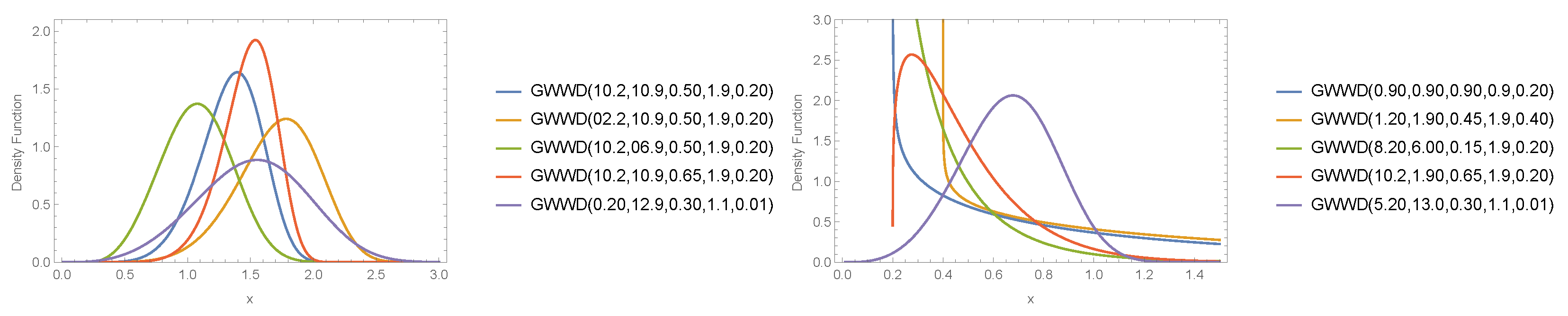
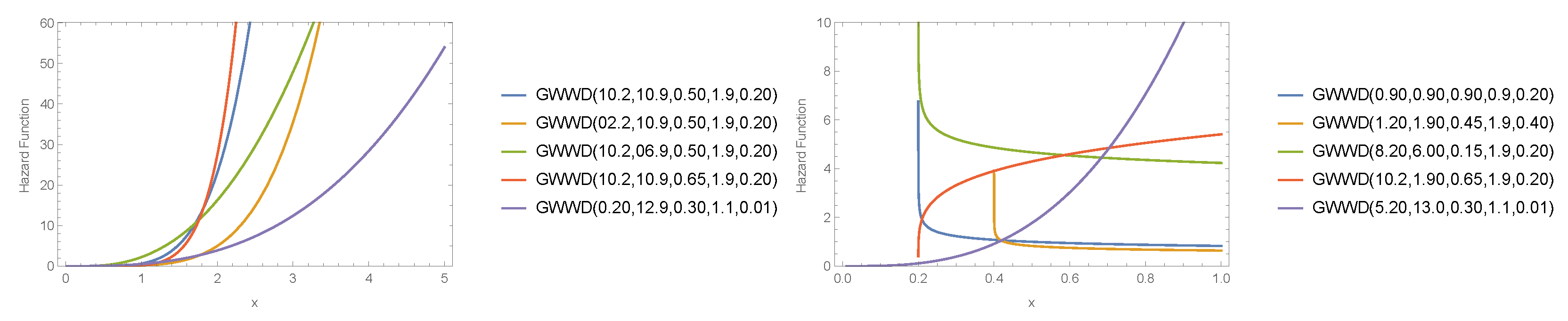
- can take several forms: a right-skewed form, a left-skewed form, a decreasing form, a curved form, and a symmetric form. The failure rate function also can take a variety of forms, so it has important standing in reliability analysis.
- (v)
- the model functions have simple and closed forms.
2. The
3. Properties of the
3.1. Quantile Function
3.2. Moments
3.3. The Information Generating Function
3.4. The Shannon Entropy (H)
3.5. The Informational Energy (IE)
4. Maximum Likelihood Estimation (MLE)
- 1.
- Generate sample from the GWWD of size n and estimate a .
- 2.
- Generate another sample of size n using . Then estimate .
- 3.
- Repeat step 2 B times.
- 4.
- Via , that is, the CDF of , the C.I. of is given bywhere and x is prefixed.
5. Bayesian Estimation
MCMC Method
- 1.
- Set start values and . Then, simulate sample of size n from GWWD , next set .
- 2.
- Simulate and . using the proposal distributions , , and .
- 3.
- Calculate r = min.
- 4.
- Simulate U from Uniform (0, 1).
- 5.
- If , then .If , then .
- 6.
- Set .
- 7.
- Iterate Steps 2–6, M repetitions, and get and for ….
- 1.
- Arrange and in rising values.
- 2.
- The lower bounds of and is in the rank .
- 3.
- The Upper bounds of and is in the rank .
- 4.
- Iterate the previous steps M times. Get the average value of the lower and upper bounds of and .
6. Simulation Study
- We generate sample of sizes n = 25, 50, 100, 200, 400, and 600 from the via initial parameter values are and .
- Again use each of the cases in step (1) for calculating the Bayesian estimates for both cases of GE, LINEX and SE loss functions. The parameter in LINEX is chosen as −3 and 7. The parameter in general entropy is chosen as 0.5.
- For the Bayesian analysis, we take small values for the hyper-parameters as .
- The steeps (1)–(3) are repeated M= 3000 times, then the estimate, bias and estimated risk (ER) in each cases are calculated in Table 2. Obtain the point estimation of the parameter using MLE and MCMC methods (with 10,000 repetitions and 200 burns).
- The and approximate confidence, bootstrap HPD credible intervals with their width are calculated.
- The biases and ERs are given, respectively, byand
- Coverage probabilities (CPs) are also calculated at the 95% and 90% HPD credible intervals. The simulation results are presented in Table 2 for the parameters and , respectively.
- In most cases, the Bayesian estimates of are overestimated, while the MLE estimates is underestimated.
- In most cases, the estimates of are overestimated.
- In most cases, the Bayesian estimates of and are underestimated, while the MLE estimates is overestimated.
- In most cases, the Bayesian estimates of is overestimated, while the MLE estimates is underestimated.
- The results shows that the Bayesian estimate based Linex with negative approach gives better estimates other Bayesian estimators.
- The performance of MLE was also good even when the small sample sizes.
- At the level of confidence intervals, there is a significant superiority the Bayesian approach.
7. Application of the
8. Discussion and Future Works
9. Concluding Remarks
Funding
Data Availability Statement
Conflicts of Interest
References
- Specht, M. Consistency of the empirical distributions of navigation positioning system errors with theoretical distributions: Comparative analysis of the DGPS and EGNOS systems in the years 2006 and 2014. Sensors 2021, 21, 31. [Google Scholar] [CrossRef] [PubMed]
- Roos, A.L.; Goetz, T.; Voracek, M.; Krannich, M.; Bieg, M.; Jarrell, A.; Pekrun, R. Test anxiety and physiological arousal: A systematic review and meta-analysis. Educ. Psychol. 2021, 33, 579–618. [Google Scholar] [CrossRef]
- Du, M.; Yuan, X. A survey of competitive sports data visualization and visual analysis. J. Vis. 2021, 24, 47–67. [Google Scholar] [CrossRef]
- Nejad, R.M.; Liu, Z.; Ma, W.; Berto, F. Reliability analysis of fatigue crack growth for rail steel under variable amplitude service loading conditions and wear. Int. J. Fatigue 2021, 152, 106450. [Google Scholar] [CrossRef]
- Bergwerk, M.; Gonen, T.; Lustig, Y.; Amit, S.; Lipsitch, M.; Cohen, C.; Regev-Yochay, G. COVID-19 breakthrough infections in vaccinated health care workers. N. Engl. J. Med. 2021, 385, 1474–1484. [Google Scholar] [CrossRef]
- Mansournia, M.A.; Nazemipour, M.; Naimi, A.I.; Collins, G.S.; Campbell, M.J. Reflection on modern methods: Demystifying robust standard errors for epidemiologists. Int. J. Epidemiol. 2021, 50, 346–351. [Google Scholar] [CrossRef] [PubMed]
- Misuraca, M.; Scepi, G.; Spano, M. Using Opinion Mining as an educational analytic: An integrated strategy for the analysis of students’ feedback. Stud. Educ. Eval. 2021, 68, 100979. [Google Scholar] [CrossRef]
- Liao, D.; Zhu, S.P.; Keshtegar, B.; Qian, G.; Wang, Q. Probabilistic framework for fatigue life assessment of notched components under size effects. Int. J. Mech. Sci. 2020, 181, 105685. [Google Scholar] [CrossRef]
- Cong, J.; Ahmad, Z.; Alsaedi, B.S.; Alamri, O.A.; Alkhairy, I.; Alsuhabi, H. The Role of Twitter Medium in Business with Regression Analysis and Statistical Modelling. Comput. Intell. Neurosci. 2021, 2021, 1–12. [Google Scholar] [CrossRef]
- Zheng, H.; Kong, X.; Xu, H.; Yang, J. Reliability analysis of products based on proportional hazard model with degradation trend and environmental factor. Reliab. Eng. Syst. Saf. 2021, 216, 107964. [Google Scholar] [CrossRef]
- Ahmad, Z.; Mahmoudi, E.; Alizadeh, M.; Roozegar, R.; Afify, A.Z. The Exponential TX Family of Distributions: Properties and an Application to Insurance Data. J. Math. 2021, 2021, 1–18. [Google Scholar]
- Almalki, S.J.; Nadarajah, S. Modifications of the Weibull distribution: A review. Reliab. Eng. Syst. 2014, 124, 32–55. [Google Scholar] [CrossRef]
- Emam, W.; Tashkandy, Y. The Weibull Claim Model: Bivariate Extension, Bayesian, and Maximum Likelihood Estimations. Math. Probl. Eng. 2022, 2022, 1–10. [Google Scholar] [CrossRef]
- Emam, W.; Tashkandy, Y. A New Generalized Modified Weibull Model: Simulating and Modeling the Dynamics of the COVID-19 Pandemic in Saudi Arabia and Egypt. Math. Probl. Eng. 2022, 2022, 1–9. [Google Scholar] [CrossRef]
- Emam, W.; Tashkandy, Y. The Arcsine Kumaraswamy-Generalized Family: Bayesian and Classical Estimates and Application. Symmetry 2022, 14, 2311. [Google Scholar] [CrossRef]
- Yousof, H.M.; Tashkandy, Y.; Emam, W.; Ali, M.M.; Ibrahim, M. A New Reciprocal Weibull Extension for Modeling Extreme Values with Risk Analysis under Insurance Data. Mathematics 2023, 11, 966. [Google Scholar] [CrossRef]
- Emam, W.; Tashkandy, Y.; Emam, W.; Goual, H.; Hamida, T.; Masoom, A.H.; Yousof, H.; Ibrahim, M. A New One-Parameter Distribution for Right Censored Bayesian and Non-Bayesian Distributional Validation under Various Estimation Methods. Mathematics 2023, 11, 897. [Google Scholar] [CrossRef]
- Emam, W.; Tashkandy, Y. Modeling the Amount of Carbon Dioxide Emissions Application: New Modified Alpha Power Weibull-X Family of Distributions. Symmetry 2023, 15, 366. [Google Scholar] [CrossRef]
- Emam, W.; Tashkandy, Y. Khalil New Generalized Weibull Distribution Based on Ranked Samples: Estimation, Mathematical Properties, and Application to COVID-19 Data. Symmetry 2022, 14, 853. [Google Scholar] [CrossRef]
- Klugman, S.A.; Panjer, H.H.; Willmot, G.E. Loss Models: From Data to Decisions, 4td ed.; Wiley Series in Probability and Statistics; John Wiley and Sons, Inc.: Hoboken, NJ, USA, 2012. [Google Scholar]
- Lane, M.N. Pricing risk transfer transactions 1. Astin Bull. 2000, 30, 259–293. [Google Scholar] [CrossRef] [Green Version]
- Cooray, K.; Ananda, M.M. Modeling actuarial data with a composite lognormal-Pareto model. Scand Actuar. J. 2005, 5, 321–334. [Google Scholar] [CrossRef]
- Ibragimov, R.; Prokhorov, A. Heavy tails and copulas: Topics in dependence modelling in economics and finance. World Sci. Connect. Great Mind 2017. [Google Scholar] [CrossRef] [Green Version]
- Bernardi, M.; Maruotti, A.; Petrella, L. Skew mixture models for loss distributions: A Bayesian approach. Insur. Math. Econ. 2012, 51, 617–623. [Google Scholar] [CrossRef] [Green Version]
- Adcock, C.; Eling, M.; Loperfido, N. Skewed distributions in finance and actuarial science: A review. Eur. J. Finan. 2015, 21, 1253–1281. [Google Scholar] [CrossRef]
- Bhati, D.; Ravi, S. On generalized log-Moyal distribution: A new heavy tailed size distribution. Insur. Math. Econ. 2018, 79, 247–259. [Google Scholar] [CrossRef]
- Cordeiro, G.M.; Ortega, E.M.M.; Ramires, T.G. A new generalized Weibull family of distributions: Mathematical properties and applications. J. Stat. Distrib. Appl. 2015, 2, 1–25. [Google Scholar] [CrossRef] [Green Version]
- Bowley, A.L. Elements of Statistics, 4th ed.; Charles Scribner’s Sons: New York, NY, USA, 1920. [Google Scholar]
- Moors, J.J.A. The meaning of kurtosis: Darlington re-examined. Am. Stat. 1986, 40, 283–284. [Google Scholar]
- Golomb, S. The IGF of a probability distribution (corresp.). IEEE Trans. Inf. Theory 1966, 12, 75–77. [Google Scholar] [CrossRef]
- López-Ruiz, R.; Mancini, H.L.; Calbet, X. A statistical measure of complexity. Phys. Lett. A 1995, 209, 321–326. [Google Scholar]
- Shannon, C. A Mathematical Theory of Communication. Bell Syst. Tech. J. 1984, 27, 623–656. [Google Scholar] [CrossRef]
- Cataron, A.; Andonie, R. How to infer the informational energy from small datasets. In Proceedings of the 2012 13th International Conference on Optimization of Electrical and Electronic Equipment (OPTIM), Brasov, Romania, 24–26 May 2012; pp. 1065–1070. [Google Scholar]
- Kundu, D.; Joarder, A. Analysis of Type-II progressively hybrid censored data. Comput. Stat. Data Anal. 2006, 50, 2509–2528. [Google Scholar] [CrossRef]
- Singpurwalla, N.D. Reliability and Risk A Bayesian Perspective; John Wiley & Sons Ltd.: Chichester, UK, 2006. [Google Scholar]
- Wong, A. Approximate studentization for Pareto distribution with application to censored data. Stat. Pap. 1998, 39, 189–201. [Google Scholar] [CrossRef]


| K | |||
|---|---|---|---|
| 0.05 | 1.1001 | 0.999998 | 3325.26 |
| 0.2 | 1.20034 | 0.938246 | 7.42379 |
| 0.4 | 1.41835 | 0.679392 | 2.44666 |
| 0.6 | 1.56778 | 0.477511 | 1.66985 |
| 0.8 | 1.66704 | 0.347893 | 1.41426 |
| 1 | 1.73644 | 0.26186 | 1.30627 |
| 3.288 | 1.97765 | 1.12 × 10 | 1.21002 |
| 3.285 | 1.97765 | 0 | 1.21002 |
| 3.289 | 1.97769 | −2.4 × 10 | 1.21003 |
| 7 | 2.04552 | −0.0628706 | 1.23677 |
| 20 | 2.08695 | −0.099024 | 1.26168 |
| 40 | 2.09841 | −0.108735 | 1.26962 |
| 60 | 2.10226 | −0.111969 | 1.27239 |
| 80 | 2.10419 | −0.113586 | 1.2738 |
| Par. | ||||||||||||
|---|---|---|---|---|---|---|---|---|---|---|---|---|
| n = 25 | 6.3181 | 10.3431 | 10.3719 | 10.2251 | 10.3209 | 4.8457 7.7905 | 4.074 12.802 | 6.084 13.773 | 6.1198 13.7789 | 5.9828 13.7537 | 6.0457 13.7704 | |
| −3.7073 | 0.3177 | 0.3465 | 0.1997 | 0.2955 | 2.9448 | 8.728 | 7.689 | 7.6591 | 7.7709 | 7.7247 | ||
| 0.5643 | 3.3109 | 3.3618 | 3.0911 | 3.2849 | 5.0785 7.5576 | 4.105 11.067 | 7.4 13.714 | 7.4354 13.7226 | 7.2949 13.5131 | 7.3673 13.6937 | ||
| 2.4791 | 6.962 | 6.314 | 6.2872 | 6.2183 | 6.3264 | |||||||
| 1.0574 | 0.7607 | 0.763 | 0.7508 | 0.7334 | 0.7306 1.3843 | 0.028 3.857 | 0.248 1.416 | 0.2481 1.4163 | 0.2481 1.3778 | 0.248 1.3543 | ||
| 1.03 | 0.7333 | 0.7355 | 0.7234 | 0.706 | 0.6537 | 3.829 | 1.168 | 1.1682 | 1.1297 | 1.1063 | ||
| 0.0278 | 0.6421 | 0.6469 | 0.6215 | 0.5927 | 0.7823 1.3326 | 0.07 2.864 | 0.331 1.356 | 0.3319 1.3622 | 0.3294 1.3177 | 0.319 1.2817 | ||
| 0.5503 | 2.794 | 1.025 | 1.0303 | 0.9883 | 0.9627 | |||||||
| 0.8828 | 0.5237 | 0.5238 | 0.5234 | 0.5224 | 0.8025 0.9631 | 0.268 2.03 | 0.371 0.632 | 0.3714 0.6324 | 0.3712 0.6321 | 0.3708 0.6319 | ||
| 0.3611 | 0.002 | 0.0021 | 0.0017 | 0.0007 | 0.1606 | 1.762 | 0.261 | 0.2611 | 0.2608 | 0.2611 | ||
| 0.0017 | 0.0049 | 0.0049 | 0.0049 | 0.0049 | 0.8152 0.9504 | 0.331 1.705 | 0.412 0.631 | 0.4116 0.6309 | 0.4114 0.6309 | 0.4108 0.6303 | ||
| 0.1352 | 1.374 | 0.219 | 0.2194 | 0.2195 | 0.2195 | |||||||
| 4.371 | 0.1072 | 0.1132 | 0.089 | 0.0312 | 3.3328 5.4092 | 0.736 7.05 | 0.004 0.442 | 0.0044 0.4616 | 0.0044 0.3357 | 0.0015 0.1187 | ||
| 3.2126 | −1.0512 | −1.0452 | −1.0694 | −1.1272 | 2.0764 | 6.314 | 0.438 | 0.4572 | 0.3314 | 0.1172 | ||
| 0.2806 | 1.1208 | 1.1116 | 1.1515 | 1.2715 | 3.497 5.245 | 1.081 6.924 | 0.009 0.366 | 0.009 0.4048 | 0.009 0.2666 | 0.0026 0.0923 | ||
| 1.748 | 5.843 | 0.357 | 0.3958 | 0.2576 | 0.0897 | |||||||
| n = 50 | 6.4887 | 10.1651 | 10.1893 | 10.0699 | 10.1456 | 5.4776 7.4997 | 4.08 13.449 | 7.103 12.454 | 7.1026 12.5488 | 7.1026 12.1554 | 7.1026 12.3822 | |
| −3.5368 | 0.1397 | 0.1639 | 0.0445 | 0.1202 | 2.0221 | 9.369 | 5.351 | 5.4462 | 5.0528 | 5.2795 | ||
| 0.2661 | 1.6401 | 1.656 | 1.5826 | 1.6381 | 5.6375 7.3398 | 4.134 11.872 | 8.057 12.057 | 8.198 12.1842 | 7.9144 11.9608 | 7.9333 12.0548 | ||
| 1.7023 | 7.738 | 4 | 3.9862 | 4.0464 | 4.1215 | |||||||
| 1.306 | 0.7934 | 0.7956 | 0.7836 | 0.7683 | 1.0508 1.5612 | 0.045 4.306 | 0.255 1.503 | 0.2555 1.507 | 0.2509 1.4554 | 0.2414 1.396 | ||
| 1.2785 | 0.766 | 0.7682 | 0.7561 | 0.7408 | 0.5103 | 4.261 | 1.248 | 1.2516 | 1.2044 | 1.1546 | ||
| 0.0169 | 0.6945 | 0.6991 | 0.6741 | 0.649 | 1.0912 1.5208 | 0.102 3.469 | 0.317 1.308 | 0.3177 1.3087 | 0.3161 1.304 | 0.3042 1.3018 | ||
| 0.4296 | 3.367 | 0.991 | 0.9909 | 0.988 | 0.9976 | |||||||
| 0.9169 | 0.518 | 0.5181 | 0.5178 | 0.5171 | 0.8625 0.9712 | 0.252 2.228 | 0.366 0.653 | 0.3665 0.6536 | 0.3661 0.6531 | 0.365 0.6523 | ||
| 0.3952 | −0.0038 | −0.0037 | −0.004 | −0.0047 | 0.1087 | 1.976 | 0.287 | 0.2871 | 0.287 | 0.2874 | ||
| 0.0008 | 0.0044 | 0.0044 | 0.0044 | 0.0045 | 0.8711 0.9626 | 0.325 1.885 | 0.404 0.628 | 0.4043 0.629 | 0.4041 0.6261 | 0.4035 0.6205 | ||
| 0.0915 | 1.56 | 0.224 | 0.2247 | 0.222 | 0.217 | |||||||
| 4.3197 | 0.1427 | 0.1506 | 0.1163 | 0.0276 | 3.6536 4.9858 | 0.55 7.035 | 0.003 0.789 | 0.0026 0.8551 | 0.0026 0.5736 | 0.0019 0.1317 | ||
| 3.1613 | −1.0156 | −1.0078 | −1.0421 | −1.1308 | 1.3322 | 6.485 | 0.786 | 0.8525 | 0.571 | 0.1298 | ||
| 0.1155 | 1.0707 | 1.0605 | 1.1081 | 1.2799 | 3.7589 4.8804 | 0.99 6.941 | 0.006 0.513 | 0.006 0.5699 | 0.006 0.3466 | 0.0023 0.1133 | ||
| 1.1215 | 5.951 | 0.507 | 0.5639 | 0.3406 | 0.111 | |||||||
| n = 100 | 6.6441 | 10.2021 | 10.2187 | 10.1356 | 10.1887 | 5.968 7.3202 | 4.063 14.199 | 6.799 12.282 | 6.8126 12.3097 | 6.7487 12.147 | 6.7835 12.2636 | |
| −3.3813 | 0.1767 | 0.1933 | 0.1102 | 0.1633 | 1.3522 | 10.136 | 5.483 | 5.4971 | 5.3983 | 5.4801 | ||
| 0.119 | 1.2782 | 1.2829 | 1.2505 | 1.2797 | 6.075 7.2133 | 4.123 12.487 | 8.245 11.876 | 8.2567 11.9168 | 8.1858 11.7579 | 8.2297 11.8457 | ||
| 1.1383 | 8.364 | 3.631 | 3.6601 | 3.5722 | 3.6159 | |||||||
| 1.6427 | 0.7726 | 0.7748 | 0.7632 | 0.7467 | 1.4372 1.8482 | 0.055 4.769 | 0.313 1.293 | 0.3128 1.2965 | 0.3127 1.2798 | 0.3125 1.1974 | ||
| 1.6152 | 0.7451 | 0.7474 | 0.7358 | 0.7193 | 0.411 | 4.714 | 0.98 | 0.9837 | 0.9671 | 0.8849 | ||
| 0.011 | 0.6226 | 0.6268 | 0.6051 | 0.5783 | 1.4697 1.8157 | 0.104 4.138 | 0.366 1.203 | 0.3686 1.2057 | 0.3616 1.1889 | 0.3514 1.1748 | ||
| 0.346 | 4.034 | 0.837 | 0.8371 | 0.8273 | 0.8234 | |||||||
| 0.9418 | 0.5157 | 0.5158 | 0.5155 | 0.5149 | 0.9056 0.978 | 0.275 2.37 | 0.426 0.61 | 0.4262 0.61 | 0.4261 0.6098 | 0.4259 0.6096 | ||
| 0.4201 | −0.006 | −0.006 | −0.0062 | −0.0068 | 0.0724 | 2.095 | 0.184 | 0.1838 | 0.1837 | 0.1837 | ||
| 0.0003 | 0.0028 | 0.0028 | 0.0028 | 0.0028 | 0.9114 0.9723 | 0.348 1.893 | 0.431 0.601 | 0.4313 0.6008 | 0.431 0.6007 | 0.4295 0.6004 | ||
| 0.0609 | 1.545 | 0.17 | 0.1695 | 0.1696 | 0.1709 | |||||||
| 4.384 | 0.232 | 0.2442 | 0.19 | 0.0368 | 3.9463 4.8216 | 0.732 7.062 | 0.009 0.785 | 0.009 0.8254 | 0.0082 0.6529 | 0.0003 0.2209 | ||
| 3.2256 | −0.9264 | −0.9142 | −0.9684 | −1.1216 | 0.8753 | 6.33 | 0.776 | 0.8164 | 0.6447 | 0.2206 | ||
| 0.0499 | 0.906 | 0.8896 | 0.968 | 1.2624 | 4.0156 4.7524 | 1.159 6.969 | 0.014 0.71 | 0.014 0.7237 | 0.0139 0.5954 | 0.0007 0.1041 | ||
| 0.7369 | 5.81 | 0.696 | 0.7097 | 0.5815 | 0.1034 | |||||||
| n = 200 | 6.7887 | 10.2314 | 10.2422 | 10.1876 | 10.2227 | 6.3275 7.2499 | 4.075 14.026 | 8.125 12.06 | 8.1681 12.0764 | 7.9705 11.9846 | 8.0848 12.0483 | |
| −3.2367 | 0.206 | 0.2168 | 0.1621 | 0.1973 | 0.9224 | 9.951 | 3.935 | 3.9083 | 4.014 | 3.9636 | ||
| 0.0554 | 0.7143 | 0.7158 | 0.704 | 0.7145 | 6.4004 7.1769 | 4.129 12.796 | 8.995 11.776 | 9.0071 11.7941 | 8.9532 11.6652 | 8.9856 11.7619 | ||
| 0.7765 | 8.667 | 2.781 | 2.787 | 2.7121 | 2.7764 | |||||||
| 1.8115 | 0.6668 | 0.6696 | 0.655 | 0.6279 | 1.6635 1.9594 | 0.05 5.23 | 0.264 1.158 | 0.2646 1.1606 | 0.2625 1.1272 | 0.2527 1.0693 | ||
| 1.784 | 0.6394 | 0.6422 | 0.6276 | 0.6004 | 0.2959 | 5.18 | 0.894 | 0.896 | 0.8647 | 0.8166 | ||
| 0.0057 | 0.4555 | 0.4599 | 0.4372 | 0.4015 | 1.6869 1.936 | 0.091 4.817 | 0.331 1.108 | 0.3311 1.1208 | 0.3293 1.0721 | 0.3208 1.0233 | ||
| 0.2491 | 4.726 | 0.777 | 0.7897 | 0.7428 | 0.7025 | |||||||
| 0.9484 | 0.5123 | 0.5123 | 0.5121 | 0.5119 | 0.9246 0.9723 | 0.261 2.43 | 0.421 0.595 | 0.4207 0.5951 | 0.4206 0.595 | 0.4203 0.5948 | ||
| 0.4267 | −0.0095 | −0.0094 | −0.0096 | −0.0099 | 0.0477 | 2.169 | 0.174 | 0.1744 | 0.1744 | 0.1744 | ||
| 0.0001 | 0.0017 | 0.0017 | 0.0017 | 0.0017 | 0.9284 0.9685 | 0.331 1.968 | 0.453 0.583 | 0.453 0.5831 | 0.4525 0.5829 | 0.4511 0.5825 | ||
| 0.0402 | 1.637 | 0.13 | 0.13 | 0.1304 | 0.1315 | |||||||
| 4.1174 | 0.3197 | 0.3323 | 0.2738 | 0.067 | 3.8483 4.3864 | 0.403 7.037 | 0.024 0.96 | 0.0248 0.9792 | 0.0225 0.8627 | 0.0012 0.5413 | ||
| 2.959 | −0.8387 | −0.8261 | −0.8846 | −1.0914 | 0.5381 | 6.634 | 0.936 | 0.9544 | 0.8402 | 0.5401 | ||
| 0.0188 | 0.7605 | 0.7429 | 0.8281 | 1.214 | 3.8909 4.3439 | 0.664 6.906 | 0.041 0.84 | 0.0415 0.8843 | 0.0391 0.7398 | 0.0015 0.1768 | ||
| 0.453 | 6.242 | 0.799 | 0.8427 | 0.7007 | 0.1754 | |||||||
| n = 400 | 6.9837 | 10.1202 | 10.1299 | 10.0817 | 10.1126 | 6.6582 7.3092 | 4.095 14.269 | 9.117 11.188 | 9.126 11.1972 | 9.0864 11.1518 | 9.1103 11.1814 | |
| -3.0417 | 0.0948 | 0.1045 | 0.0563 | 0.0872 | 0.651 | 10.174 | 2.071 | 2.0712 | 2.0653 | 2.0711 | ||
| 0.0276 | 0.3253 | 0.3287 | 0.3134 | 0.3233 | 6.7097 7.2577 | 4.151 13.153 | 9.229 11.057 | 9.2409 11.06 | 9.1831 11.0046 | 9.2188 11.0555 | ||
| 0.548 | 9.002 | 1.828 | 1.819 | 1.8216 | 1.8366 | |||||||
| 1.9108 | 0.5999 | 0.6029 | 0.5873 | 0.5508 | 1.8052 2.0165 | 0.029 5.514 | 0.297 0.97 | 0.297 0.9733 | 0.2951 0.9582 | 0.2851 0.9249 | ||
| 1.8834 | 0.5724 | 0.5755 | 0.5599 | 0.5234 | 0.2113 | 5.485 | 0.673 | 0.6762 | 0.6632 | 0.6398 | ||
| 0.0029 | 0.355 | 0.359 | 0.3387 | 0.2978 | 1.8219 1.9998 | 0.074 4.987 | 0.354 0.913 | 0.3542 0.9171 | 0.353 0.8986 | 0.341 0.8709 | ||
| 0.1779 | 4.913 | 0.559 | 0.5628 | 0.5456 | 0.5299 | |||||||
| 0.9527 | 0.513 | 0.5131 | 0.513 | 0.5127 | 0.9363 0.9692 | 0.282 2.319 | 0.444 0.557 | 0.4441 0.5575 | 0.4441 0.5572 | 0.4441 0.5567 | ||
| 0.431 | −0.0087 | −0.0087 | −0.0088 | −0.009 | 0.033 | 2.037 | 0.113 | 0.1134 | 0.1131 | 0.1127 | ||
| 0.0001 | 0.0009 | 0.0009 | 0.0009 | 0.0009 | 0.9389 0.9666 | 0.35 2.014 | 0.46 0.555 | 0.46 0.5552 | 0.4595 0.5552 | 0.4581 0.5552 | ||
| 0.0278 | 1.664 | 0.095 | 0.0952 | 0.0957 | 0.0971 | |||||||
| 4.103 | 0.5107 | 0.5225 | 0.4656 | 0.2524 | 3.9184 4.2876 | 0.388 7.018 | 0.06 1.25 | 0.0602 1.2675 | 0.0584 1.2317 | 0.0043 1.2211 | ||
| 2.9446 | −0.6477 | −0.6359 | −0.6928 | -0.906 | 0.3692 | 6.63 | 1.19 | 1.2073 | 1.1733 | 1.2168 | ||
| 0.0089 | 0.5143 | 0.4997 | 0.5724 | 0.953 | 3.9476 4.2584 | 0.764 6.867 | 0.097 1.146 | 0.0995 1.148 | 0.0867 1.1402 | 0.0054 1.0922 | ||
| 0.3108 | 6.103 | 1.049 | 1.0486 | 1.0535 | 1.0868 | |||||||
| n = 600 | 7.058 | 10.1735 | 10.1822 | 10.1382 | 10.1667 | 6.7917 7.3242 | 4.064 14.518 | 9.206 11.574 | 9.2141 11.6015 | 9.1754 11.3311 | 9.1988 11.5544 | |
| −2.9674 | 0.1481 | 0.1568 | 0.1128 | 0.1413 | 0.5324 | 10.454 | 2.368 | 2.3874 | 2.1557 | 2.3556 | ||
| 0.0184 | 0.3736 | 0.382 | 0.342 | 0.3681 | 6.8339 7.2821 | 4.125 13.313 | 9.296 11.245 | 9.2976 11.2547 | 9.2714 11.2005 | 9.2924 11.2372 | ||
| 0.4482 | 9.188 | 1.949 | 1.957 | 1.9291 | 1.9448 | |||||||
| 1.8777 | 0.5827 | 0.5865 | 0.5669 | 0.5185 | 1.7953 1.9601 | 0.025 5.605 | 0.317 0.834 | 0.3181 0.8409 | 0.3126 0.8068 | 0.2643 0.7471 | ||
| 1.8503 | 0.5552 | 0.5591 | 0.5395 | 0.491 | 0.1648 | 5.58 | 0.517 | 0.5228 | 0.4942 | 0.4828 | ||
| 0.0018 | 0.3266 | 0.3314 | 0.3076 | 0.2572 | 1.8083 1.9471 | 0.06 4.97 | 0.356 0.827 | 0.3567 0.8342 | 0.354 0.7973 | 0.3023 0.7436 | ||
| 0.1388 | 4.91 | 0.471 | 0.4775 | 0.4433 | 0.4413 | |||||||
| 0.9365 | 0.5151 | 0.5151 | 0.515 | 0.5149 | 0.9237 0.9494 | 0.247 2.501 | 0.469 0.558 | 0.4694 0.5577 | 0.4691 0.5576 | 0.4686 0.5572 | ||
| 0.4148 | −0.0066 | −0.0066 | −0.0067 | −0.0068 | 0.0257 | 2.254 | 0.089 | 0.0884 | 0.0884 | 0.0886 | ||
| 0 | 0.0005 | 0.0005 | 0.0005 | 0.0005 | 0.9257 0.9474 | 0.323 1.894 | 0.483 0.548 | 0.4826 0.5482 | 0.4824 0.548 | 0.4817 0.5477 | ||
| 0.0217 | 1.571 | 0.065 | 0.0656 | 0.0657 | 0.066 | |||||||
| 3.8824 | 0.7874 | 0.7952 | 0.7561 | 0.626 | 3.7438 4.021 | 0.345 6.939 | 0.202 1.215 | 0.2073 1.22 | 0.182 1.1943 | 0.0051 1.1814 | ||
| 2.724 | −0.371 | −0.3632 | −0.4023 | −0.5324 | 0.2772 | 6.594 | 1.013 | 1.0127 | 1.0123 | 1.1764 | ||
| 0.005 | 0.2101 | 0.203 | 0.2401 | 0.433 | 3.7657 3.9991 | 0.658 6.754 | 0.357 1.168 | 0.3735 1.1817 | 0.2946 1.1593 | 0.0135 1.1406 | ||
| 0.2333 | 6.096 | 0.811 | 0.8082 | 0.8647 | 1.127 | |||||||
| Par. | a | b | |||||
|---|---|---|---|---|---|---|---|
| 0.578219 | 0.74522 | 0.0108 | 0.1947 | 0.1953 | 0.1923 | 0.158 | |
| −3.2434 | −3.0594 | −3.0588 | −3.0618 | −3.0962 | |||
| 0.0027 | 9.3677 | 9.3641 | 9.3822 | 9.5934 | |||
| 0.774842 | 0.22833 | 0.0154 | 2.626 | 2.6799 | 2.399 | 2.4024 | |
| −0.4222 | 2.1883 | 2.2422 | 1.9613 | 1.9648 | |||
| 0.1582 | 5.1654 | 5.4436 | 4.1231 | 4.2406 | |||
| 0.866376 | 0.039942 | 0.5483 | 0.5499 | 0.5499 | 0.5499 | 0.5499 | |
| −1.9734 | −1.9718 | −1.9718 | −1.9718 | −1.9718 | |||
| 0.001 | 3.8882 | 3.8881 | 3.8882 | 3.8884 | |||
| 0.536458 | 0.645524 | 0.0046 | 0.0034 | 0.0034 | 0.0034 | 0.0025 | |
| −1.8343 | −1.8355 | −1.8355 | −1.8355 | −1.8364 | |||
| 0.001 | 3.369 | 3.3689 | 3.3689 | 3.3724 | |||
| Par. | a | b | |||||
|---|---|---|---|---|---|---|---|
| 0.578219 | 0.74522 | 0.001 0.1123 | 0.051 0.348 | 0.0515 0.3487 | 0.0507 0.3439 | 0.019 0.3077 | |
| 0.1113 | 0.297 | 0.2972 | 0.2932 | 0.2887 | |||
| 0.001 0.0962 | 0.06 0.331 | 0.0607 0.3314 | 0.0595 0.3272 | 0.0328 0.3004 | |||
| 0.0952 | 0.271 | 0.2707 | 0.2677 | 0.2676 | |||
| 0.774842 | 0.22833 | 0.001 0.795 | 1.568 3.846 | 1.5815 4.0513 | 1.4289 3.443 | 1.2721 3.5939 | |
| 0.794 | 2.278 | 2.4698 | 2.0141 | 2.3218 | |||
| 0.001 0.6717 | 1.719 3.787 | 1.7276 3.8726 | 1.6032 3.3122 | 1.3592 3.4139 | |||
| 0.6707 | 2.068 | 2.145 | 1.709 | 2.0546 | |||
| 0.866376 | 0.039942 | 0.5377 0.5589 | 0.515 0.58 | 0.5148 0.5802 | 0.5148 0.5802 | 0.5147 0.5802 | |
| 0.0213 | 0.065 | 0.0654 | 0.0654 | 0.0655 | |||
| 0.5393 0.5572 | 0.525 0.575 | 0.5249 0.5752 | 0.5249 0.5751 | 0.5248 0.5749 | |||
| 0.0179 | 0.05 | 0.0503 | 0.0502 | 0.0501 | |||
| 0.536458 | 0.645524 | 0.0017 0.0074 | 0.001 0.01 | 0.0002 0.0104 | 0.0002 0.0104 | 0.001 0.0102 | |
| 0.0057 | 0.009 | 0.0102 | 0.0102 | 0.0092 | |||
| 0.0022 0.007 | 0.001 0.01 | 0.0002 0.0099 | 0.0002 0.0099 | 0.001 0.0097 | |||
| 0.0048 | 0.009 | 0.0097 | 0.0097 | 0.0087 | |||
| Model | KS | p-Value |
|---|---|---|
| 0.15252 | 0.9476 | |
| GW-OWD | 0.21753 | 0.6559 |
| EXP-CD | 0.22573 | 0.6116 |
| TW-D | 0.26447 | 0.4142 |
| Par. | a | b | |||||
|---|---|---|---|---|---|---|---|
| 0.241816 | 0.521228 | 0.4401 | 0.1312 | 0.1318 | 0.1292 | 0.1068 | |
| −2.814 | −3.1229 | −3.1223 | −3.125 | −3.1473 | |||
| 0.3444 | 9.7559 | 9.7525 | 9.7687 | 9.9083 | |||
| 0.104293 | 0.476433 | 0.1949 | 0.4171 | 0.4181 | 0.4135 | 0.4034 | |
| 1.4649 | 0.9716 | 0.9684 | 0.9837 | 0.9958 | |||
| 0.0001 | 1.2135 | 1.2084 | 1.233 | 1.2613 | |||
| 0.020871 | 0.796755 | 1.61 | 1.4092 | 1.5439 | 1.0328 | 0.7481 | |
| 1.1723 | 0.9715 | 1.1062 | 0.5952 | 0.3105 | |||
| 2169.2 | 1.4276 | 1.7777 | 0.648 | 0.4358 | |||
| 0.764295 | 0.747721 | 0.5833 | 0.8495 | 0.8565 | 0.8213 | 0.7738 | |
| −1.2555 | −0.9894 | −0.9824 | −1.0176 | −1.065 | |||
| 0.0853 | 1.2636 | 1.2578 | 1.2885 | 1.4146 | |||
| Par. | a | b | |||||
|---|---|---|---|---|---|---|---|
| 0.241816 | 0.521228 | −0.7101 1.5903 | 0.039 0.268 | 0.0386 0.2701 | 0.0383 0.2571 | 0.0237 0.2036 | |
| 2.3003 | 0.229 | 0.2315 | 0.2188 | 0.1798 | |||
| −0.5282 1.4084 | 0.043 0.241 | 0.0433 0.2424 | 0.0433 0.2344 | 0.031 0.1875 | |||
| 1.9365 | 0.198 | 0.1991 | 0.1911 | 0.1565 | |||
| 0.104293 | 0.476433 | 0.0568 0.3928 | 0.1497 0.8421 | 0.1503 0.8439 | 0.1495 0.8371 | 0.1468 0.8244 | |
| 0.3359 | 0.6924 | 0.6935 | 0.6876 | 0.6775 | |||
| 0.0747 0.3576 | 0.1800 0.8080 | 0.1798 0.8112 | 0.1792 0.7962 | 0.1748 0.7854 | |||
| 0.2828 | 0.6279 | 0.6313 | 0.6169 | 0.6106 | |||
| 0.020871 | 0.796755 | -89.67 92.89 | 0.016 2.582 | 0.0159 2.8682 | 0.0159 2.1998 | 0.0134 2.103 | |
| 182.574 | 2.566 | 2.8523 | 2.1839 | 2.0896 | |||
| −75.2386 78.45 | 0.369 2.504 | 0.418 2.6762 | 0.2734 1.92 | 0.0386 1.8855 | |||
| 153.697 | 2.135 | 2.2583 | 1.6467 | 1.8469 | |||
| 0.764295 | 0.747721 | 0.011 1.1556 | 0.188 1.976 | 0.1964 1.9812 | 0.1638 1.9556 | 0.0951 1.9545 | |
| 1.1446 | 1.788 | 1.7848 | 1.7918 | 1.8594 | |||
| 0.1015 1.0651 | 0.276 1.703 | 0.2779 1.7123 | 0.2657 1.6623 | 0.1272 1.6482 | |||
| 0.9636 | 1.427 | 1.4345 | 1.3966 | 1.5209 | |||
| Model | KS | p-Value |
|---|---|---|
| 0.52541 | 0.0001215 | |
| GW-OWD | 0.57143 | 1.797 × 10 |
| EXP-WD | 0.85718 | 6.106 × 10 |
| TW-D | 0.53245 | 9.201 × 10 |
Disclaimer/Publisher’s Note: The statements, opinions and data contained in all publications are solely those of the individual author(s) and contributor(s) and not of MDPI and/or the editor(s). MDPI and/or the editor(s) disclaim responsibility for any injury to people or property resulting from any ideas, methods, instructions or products referred to in the content. |
© 2023 by the author. Licensee MDPI, Basel, Switzerland. This article is an open access article distributed under the terms and conditions of the Creative Commons Attribution (CC BY) license (https://creativecommons.org/licenses/by/4.0/).
Share and Cite
Emam, W. On Statistical Modeling Using a New Version of the Flexible Weibull Model: Bayesian, Maximum Likelihood Estimates, and Distributional Properties with Applications in the Actuarial and Engineering Fields. Symmetry 2023, 15, 560. https://doi.org/10.3390/sym15020560
Emam W. On Statistical Modeling Using a New Version of the Flexible Weibull Model: Bayesian, Maximum Likelihood Estimates, and Distributional Properties with Applications in the Actuarial and Engineering Fields. Symmetry. 2023; 15(2):560. https://doi.org/10.3390/sym15020560
Chicago/Turabian StyleEmam, Walid. 2023. "On Statistical Modeling Using a New Version of the Flexible Weibull Model: Bayesian, Maximum Likelihood Estimates, and Distributional Properties with Applications in the Actuarial and Engineering Fields" Symmetry 15, no. 2: 560. https://doi.org/10.3390/sym15020560