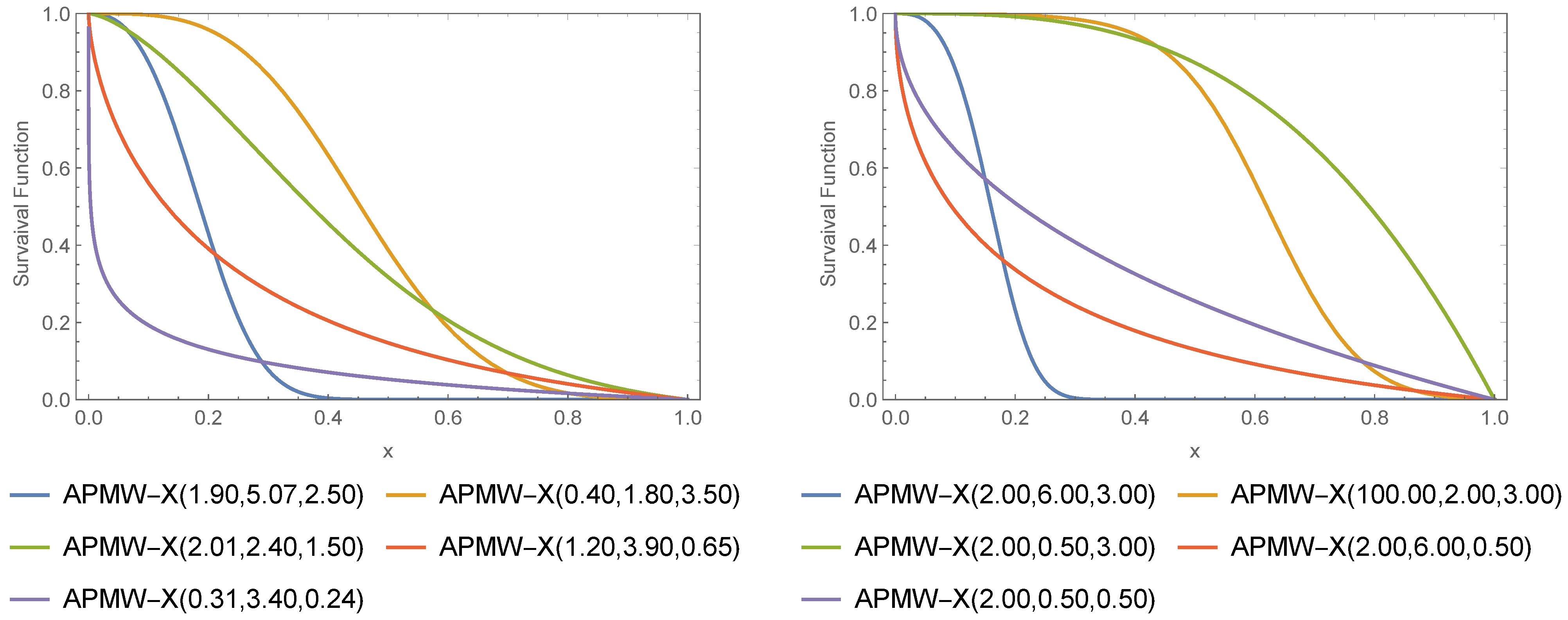
Figure 1.
Different SF for the APMW-X .
Figure 1.
Different SF for the APMW-X .
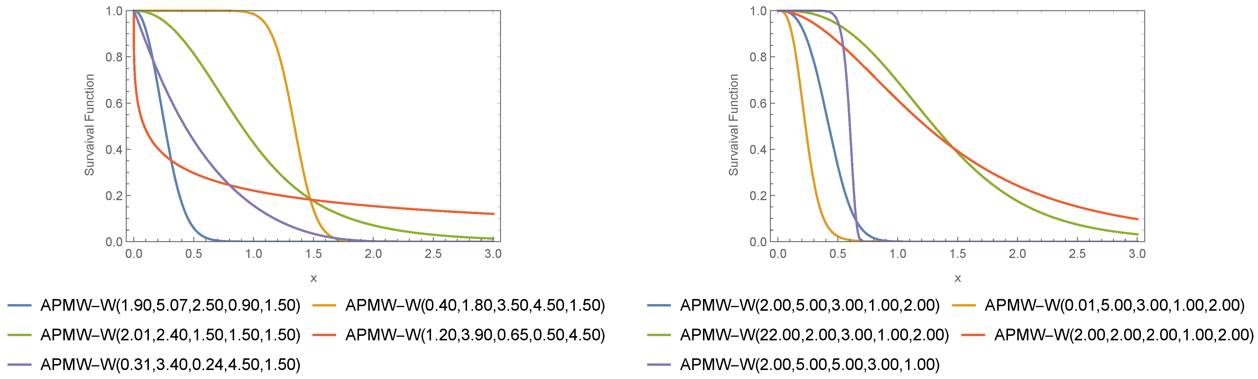
Figure 2.
Different SF for the APMW-X .
Figure 2.
Different SF for the APMW-X .
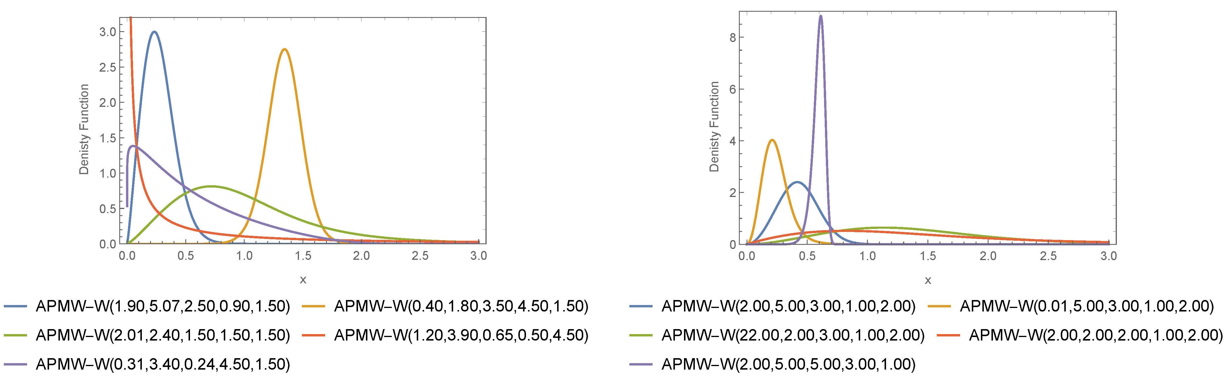
Figure 3.
Different PDF for the APMW-X .
Figure 3.
Different PDF for the APMW-X .
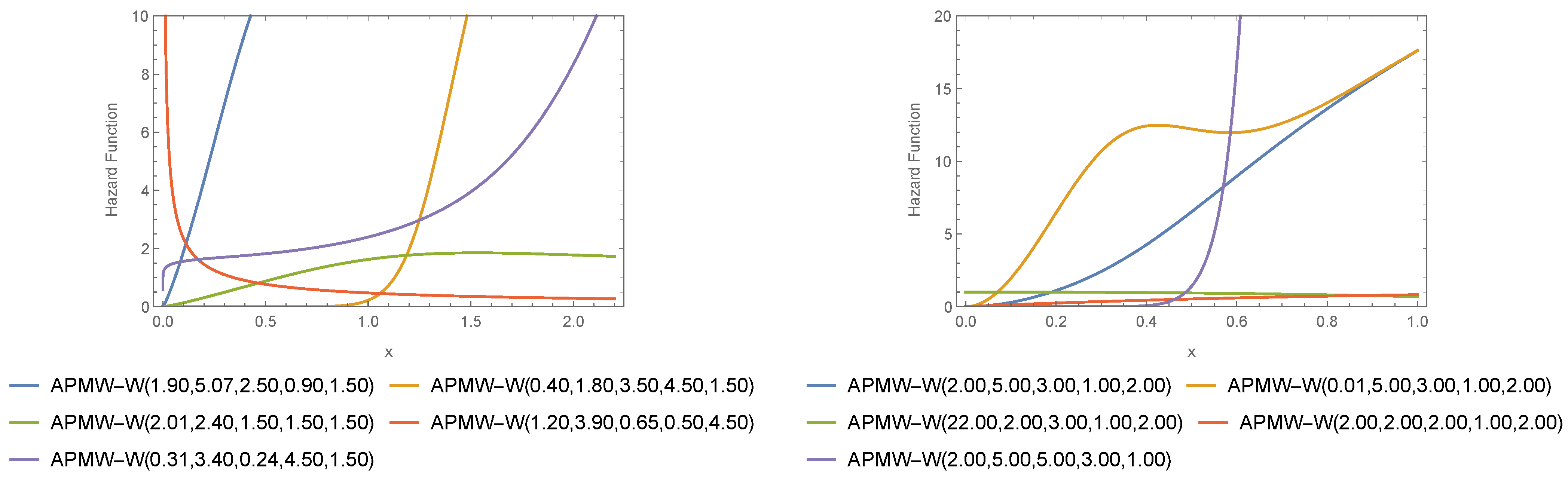
Figure 4.
Different HRF for the APMW-X .
Figure 4.
Different HRF for the APMW-X .
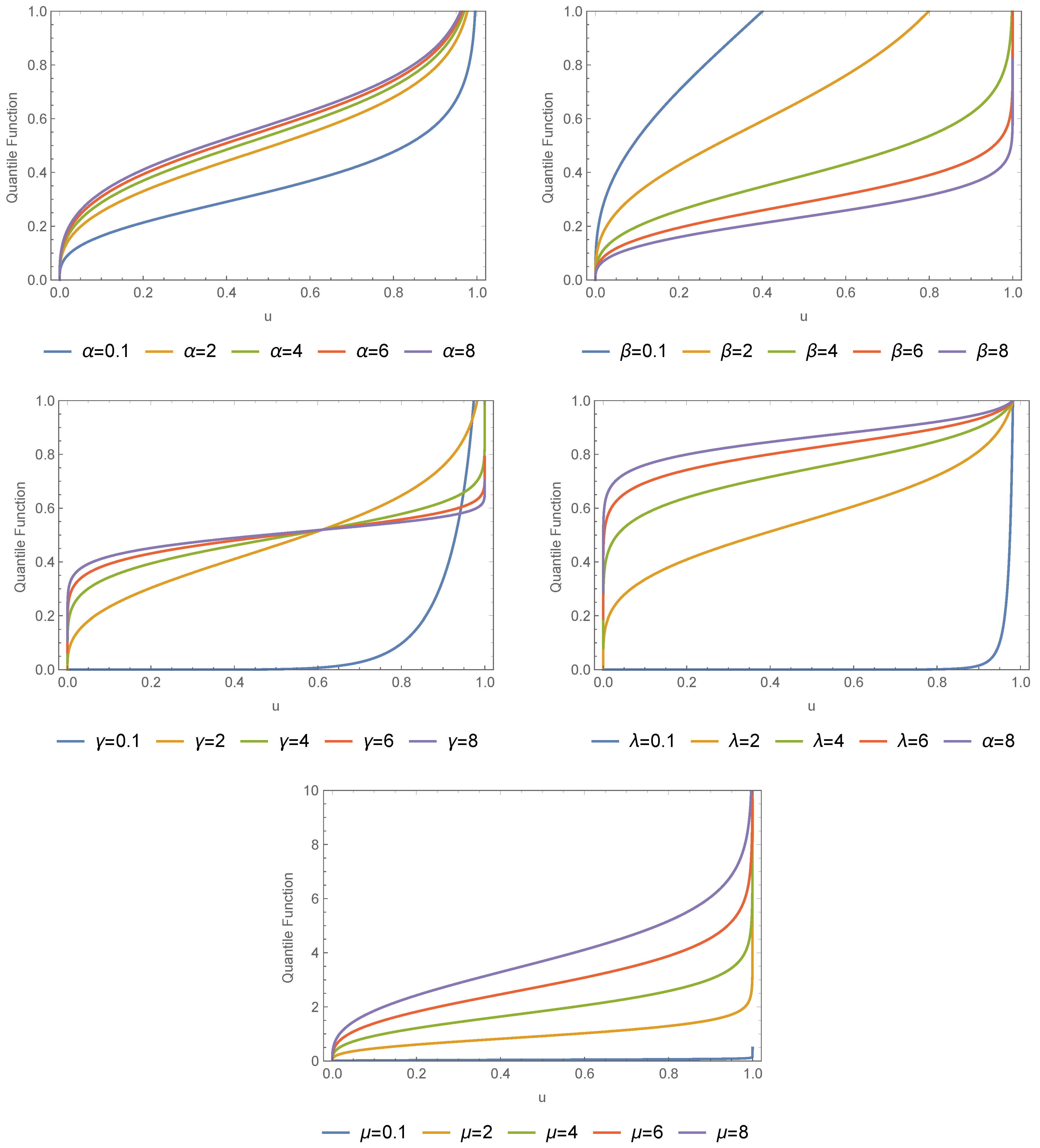
Figure 5.
Different quantile functions for the APMW-X .
Figure 5.
Different quantile functions for the APMW-X .
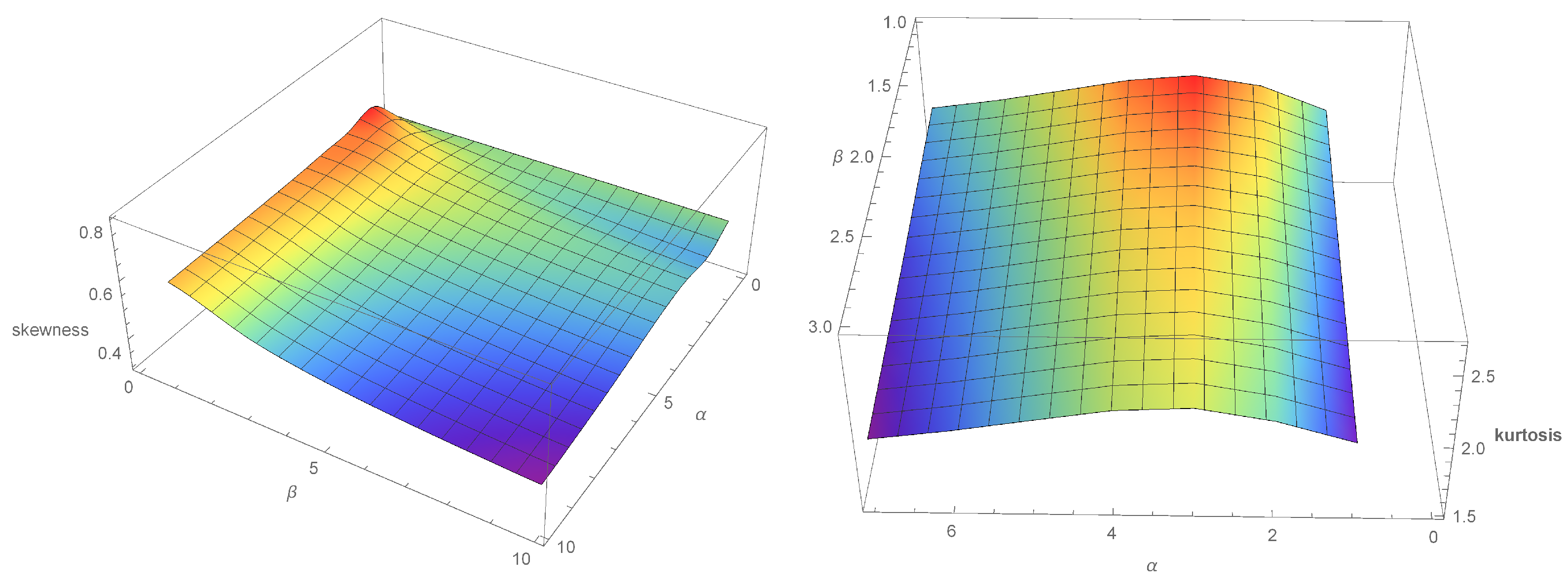
Figure 6.
Plots for the and .
Figure 6.
Plots for the and .
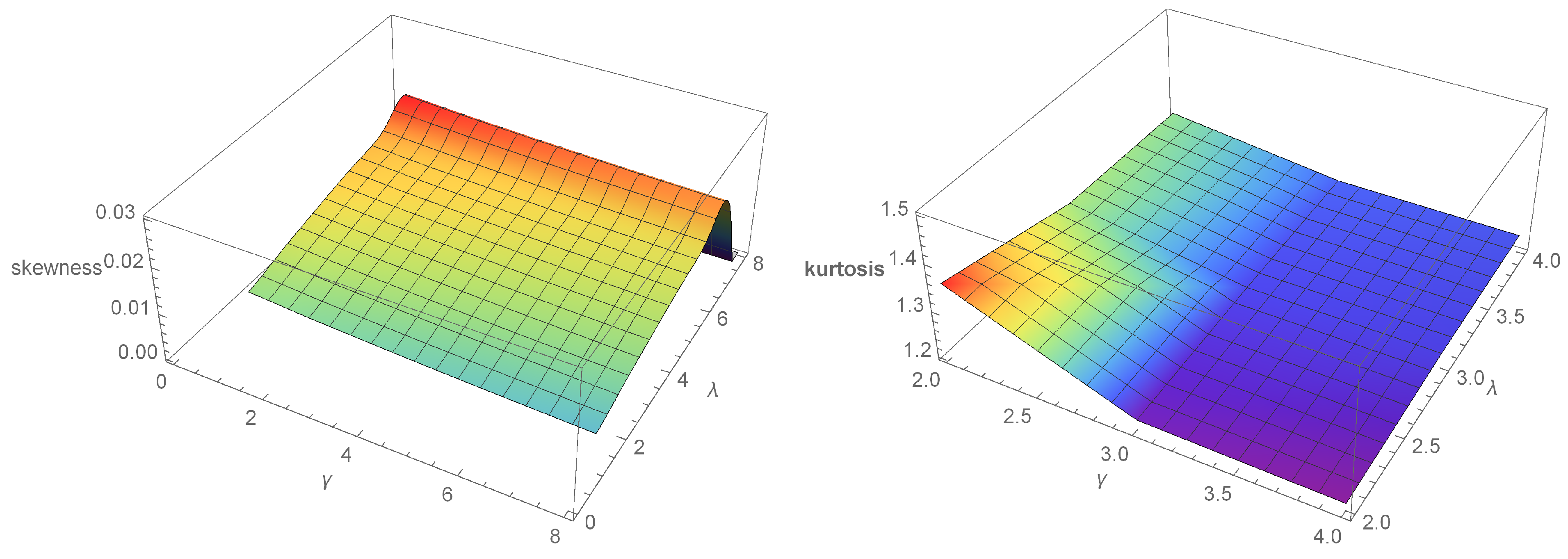
Figure 7.
Plots for the and .
Figure 7.
Plots for the and .
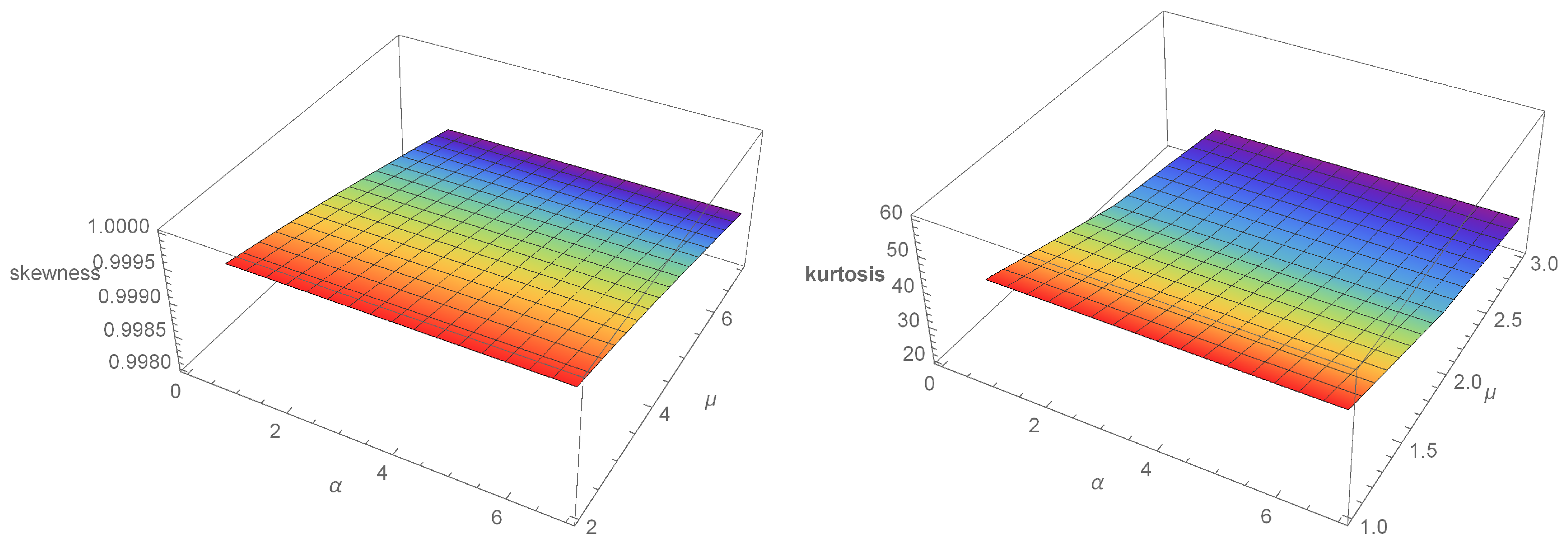
Figure 8.
Plots for the and .
Figure 8.
Plots for the and .
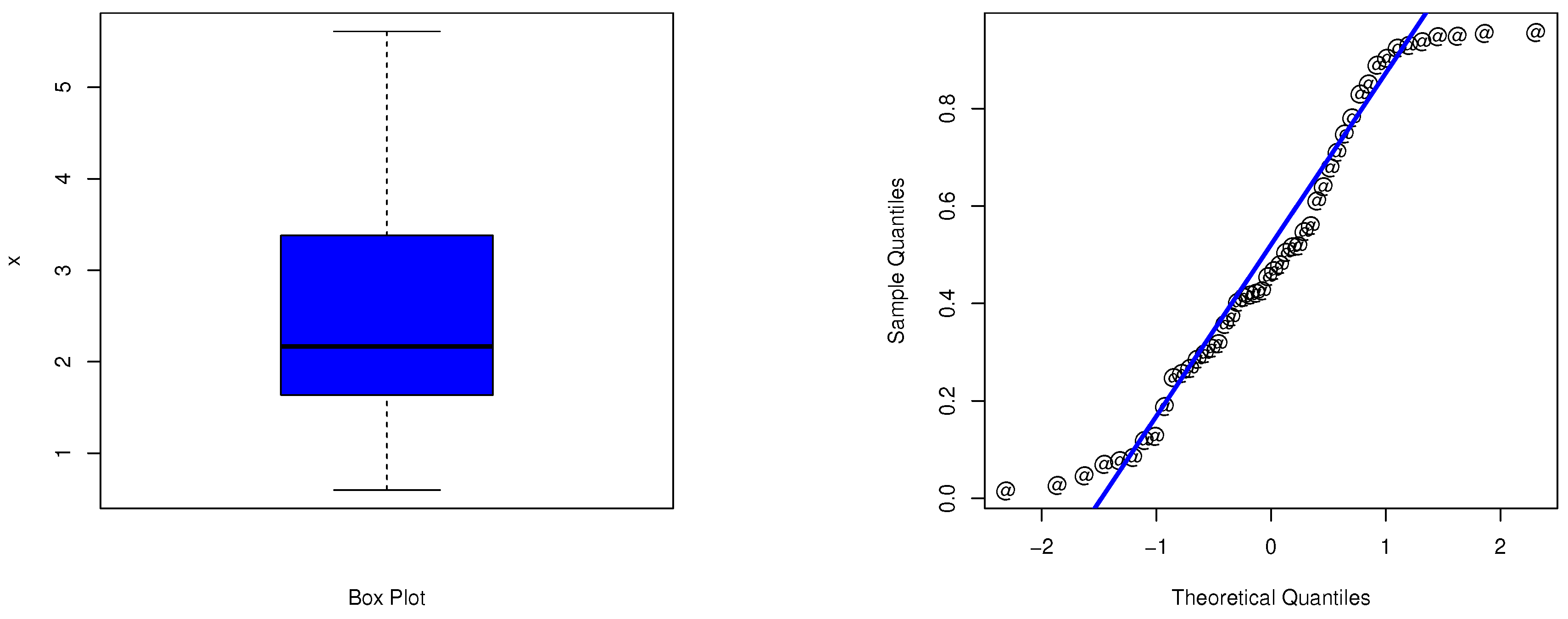
Figure 9.
The boxplot and Q-Q plot of the carbon dioxide emissions data.
Figure 9.
The boxplot and Q-Q plot of the carbon dioxide emissions data.
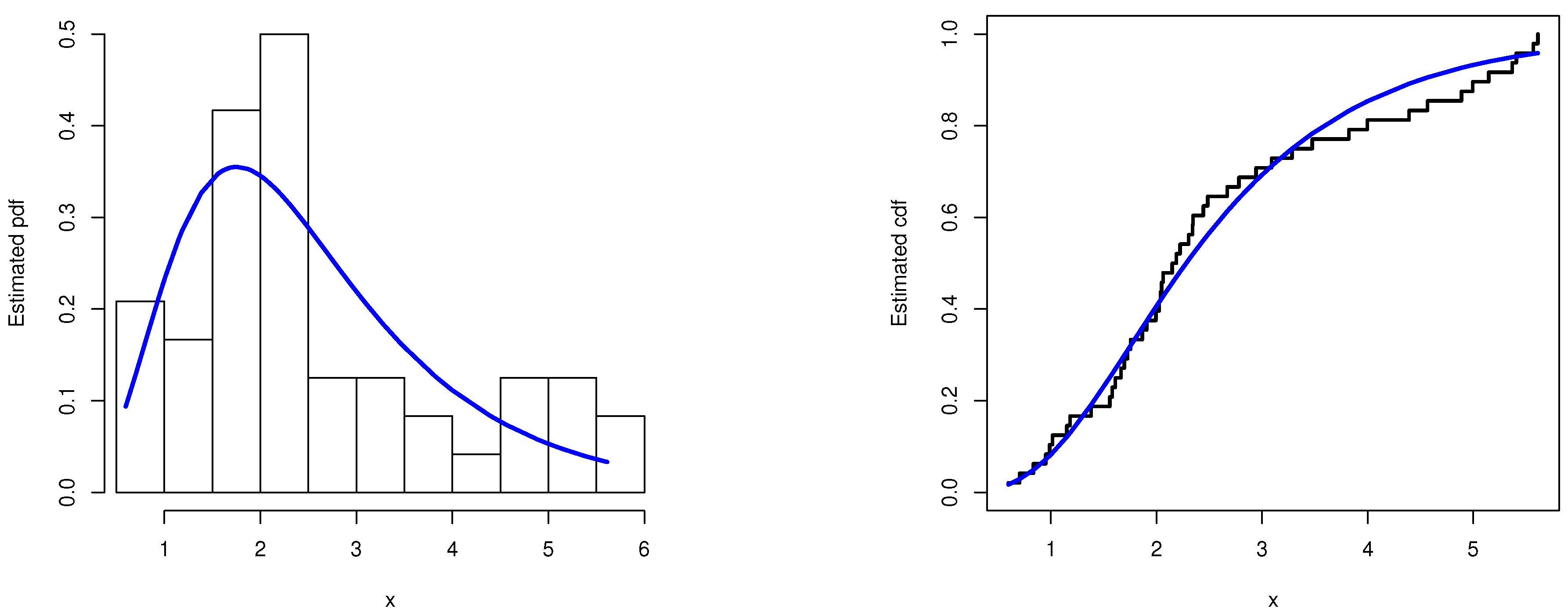
Figure 10.
The fitted PDF and CDF of the APMW-W distribution.
Figure 10.
The fitted PDF and CDF of the APMW-W distribution.
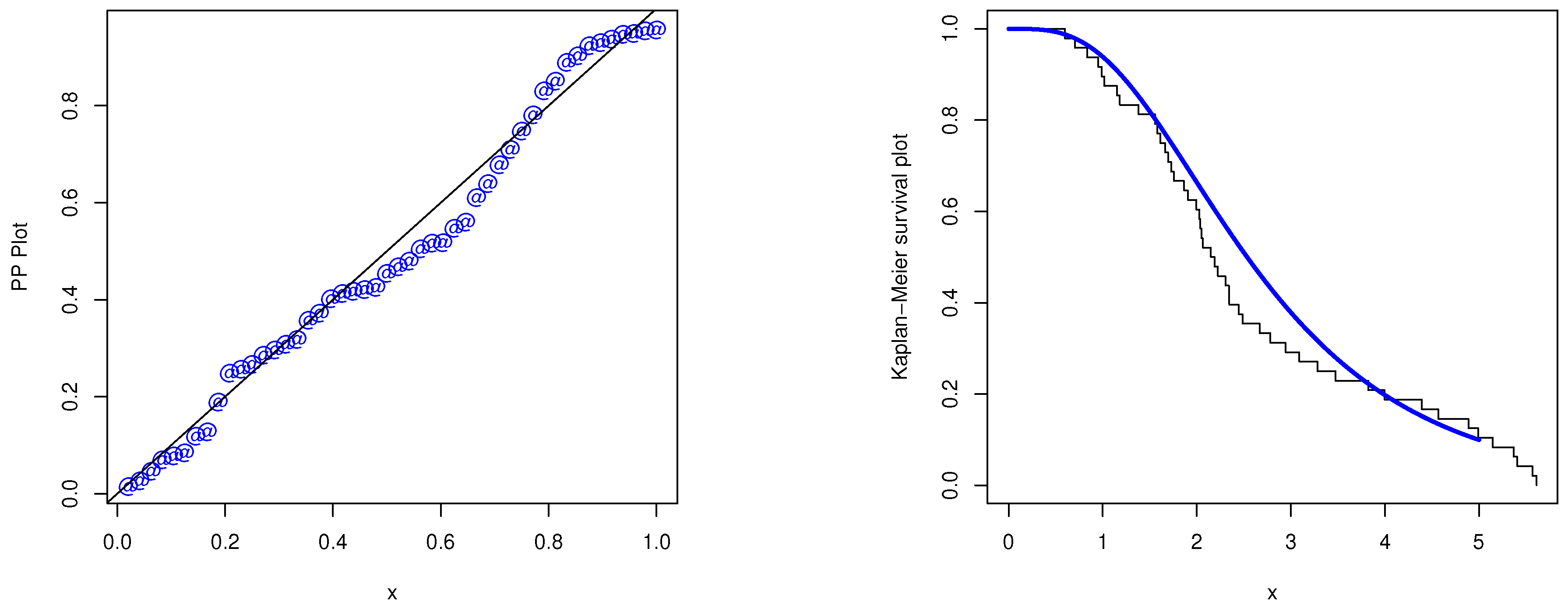
Figure 11.
The PP plot and the Kaplan–Meier survival function of the APMW-W distribution.
Figure 11.
The PP plot and the Kaplan–Meier survival function of the APMW-W distribution.
Table 1.
Some quantile values for and .
Table 1.
Some quantile values for and .
| x | Q(x) |
|---|
| 0.1 | 0.0051 |
| 0.2 | 0.0223 |
| 0.3 | 0.0557 |
| 0.4 | 0.1125 |
| 0.5 | 0.2062 |
| 0.6 | 0.3630 |
| 0.7 | 0.6420 |
| 0.8 | 1.2066 |
| 0.9 | 2.7380 |
Table 2.
Point estimation of the APMW-W parameters.
Table 2.
Point estimation of the APMW-W parameters.
| | | Point |
|---|
| n | Par. | | | | | |
|---|
| 25 | | 0.9692 | 0.7506 | 0.7686 | 0.6826 | 0.5059 |
| −0.0562 | −0.2748 | −0.2568 | −0.3428 | −0.5196 |
| 0.2838 | 0.3768 | 0.3755 | 0.392 | 0.5872 |
| 1.5303 | 1.7643 | 1.7764 | 1.7169 | 1.6556 |
| −0.4718 | −0.2378 | −0.2257 | −0.2852 | −0.3465 |
| 0.0798 | 0.3055 | 0.2913 | 0.3632 | 0.524 |
| 1.5155 | 3.2514 | 3.2528 | 3.2459 | 3.248 |
| −1.7589 | −0.023 | −0.0216 | −0.0284 | −0.0264 |
| 0.0196 | 0.0454 | 0.0453 | 0.046 | 0.046 |
| 1.7276 | 0.5805 | 0.5813 | 0.5775 | 0.5704 |
| 1.2059 | 0.0588 | 0.0596 | 0.0558 | 0.0487 |
| 0.0168 | 0.008 | 0.0082 | 0.0076 | 0.0068 |
| 1.118 | 1.1596 | 1.1682 | 1.1257 | 1.0898 |
| −0.0404 | 0.0012 | 0.0098 | −0.0327 | −0.0686 |
| | 0.0613 | 0.3122 | 0.3145 | 0.3041 | 0.3352 |
| 50 | | 1.0283 | 0.7431 | 0.7716 | 0.6462 | 0.5068 |
| 0.0029 | −0.2823 | −0.2538 | −0.3792 | −0.5186 |
| 0.1359 | 0.5382 | 0.5651 | 0.4816 | 0.6411 |
| 1.6051 | 2.0279 | 2.0325 | 2.0095 | 2.0089 |
| −0.3969 | 0.0258 | 0.0305 | 0.0075 | 0.0069 |
| 0.1304 | 0.1104 | 0.1109 | 0.1093 | 0.1118 |
| 1.4153 | 3.1505 | 3.1572 | 3.1235 | 3.1312 |
| −1.8591 | −0.1238 | −0.1171 | −0.1508 | −0.1431 |
| 0.0069 | 0.2989 | 0.2947 | 0.317 | 0.316 |
| 1.5491 | 0.6118 | 0.6124 | 0.6091 | 0.6038 |
| 1.0274 | 0.09 | 0.0907 | 0.0874 | 0.0821 |
| 0.0276 | 0.0225 | 0.0227 | 0.0215 | 0.0202 |
| 1.1025 | 1.1948 | 1.2022 | 1.165 | 1.1439 |
| −0.0559 | 0.0365 | 0.0438 | 0.0066 | −0.0145 |
| | 0.0438 | 0.2613 | 0.2658 | 0.2447 | 0.253 |
| 100 | | 0.8942 | 0.646 | 0.6587 | 0.5986 | 0.4777 |
| −0.1312 | −0.3794 | −0.3667 | −0.4268 | −0.5477 |
| 0.0881 | 0.3193 | 0.3151 | 0.3385 | 0.4707 |
| 1.6546 | 1.9359 | 1.9392 | 1.9228 | 1.9196 |
| −0.3475 | −0.0661 | −0.0628 | −0.0792 | −0.0824 |
| 0.0149 | 0.0943 | 0.093 | 0.0992 | 0.1072 |
| 1.4817 | 3.3443 | 3.3474 | 3.3322 | 3.337 |
| −1.7926 | 0.07 | 0.073 | 0.0578 | 0.0627 |
| 0.0136 | 0.1198 | 0.1205 | 0.1172 | 0.1188 |
| 1.3493 | 0.5699 | 0.5702 | 0.569 | 0.5667 |
| 0.8276 | 0.0482 | 0.0485 | 0.0473 | 0.045 |
| 0.006 | 0.0065 | 0.0065 | 0.0063 | 0.0061 |
| 1.1181 | 1.2964 | 1.3043 | 1.2657 | 1.2507 |
| −0.0402 | 0.138 | 0.1459 | 0.1073 | 0.0924 |
| | 0.0268 | 0.2139 | 0.2207 | 0.1898 | 0.1938 |
| 200 | | 1.0492 | 1.0878 | 1.0996 | 1.0403 | 0.9805 |
| 0.0238 | 0.0624 | 0.0742 | 0.0149 | −0.0449 |
| 0.0627 | 0.3592 | 0.3685 | 0.3249 | 0.3654 |
| 1.7663 | 1.9187 | 1.9211 | 1.9093 | 1.9087 |
| −0.2357 | −0.0833 | −0.0809 | −0.0928 | −0.0933 |
| 0.0309 | 0.0456 | 0.0454 | 0.0466 | 0.0474 |
| 1.4698 | 3.1943 | 3.1971 | 3.1834 | 3.1869 |
| −1.8046 | −0.0801 | −0.0773 | −0.091 | −0.0875 |
| 0.0091 | 0.0838 | 0.0823 | 0.0896 | 0.0883 |
| 1.2558 | 0.5741 | 0.5743 | 0.5734 | 0.5717 |
| 0.7341 | 0.0524 | 0.0526 | 0.0517 | 0.05 |
| 0.0026 | 0.0058 | 0.0059 | 0.0057 | 0.0054 |
| 1.1357 | 1.0035 | 1.0071 | 0.9898 | 0.9744 |
| −0.0227 | −0.1548 | −0.1513 | −0.1686 | −0.184 |
| 0.0222 | 0.116 | 0.1154 | 0.1189 | 0.1284 |
| 400 | | 0.9448 | 1.0808 | 1.0865 | 1.0583 | 1.0335 |
| −0.0806 | 0.0554 | 0.0611 | 0.0329 | 0.0081 |
| 0.0299 | 0.1758 | 0.1776 | 0.1693 | 0.1815 |
| 1.7559 | 2.0258 | 2.0268 | 2.0217 | 2.0218 |
| −0.2462 | 0.0237 | 0.0247 | 0.0196 | 0.0197 |
| 0.0163 | 0.0276 | 0.0277 | 0.0271 | 0.0272 |
| 1.4501 | 3.2464 | 3.2479 | 3.2406 | 3.2427 |
| −1.8243 | −0.0279 | −0.0265 | −0.0338 | −0.0317 |
| 0.0059 | 0.0413 | 0.041 | 0.0424 | 0.0421 |
| 1.2178 | 0.5707 | 0.5708 | 0.5704 | 0.5697 |
| 0.6961 | 0.049 | 0.0491 | 0.0487 | 0.048 |
| 0.0015 | 0.0037 | 0.0037 | 0.0036 | 0.0035 |
| 1.181 | 1.1492 | 1.1515 | 1.1403 | 1.1341 |
| 0.0227 | −0.0092 | −0.0069 | −0.0181 | −0.0243 |
| 0.0136 | 0.0602 | 0.0606 | 0.0587 | 0.0593 |
Table 3.
Interval estimation of the APMW-W parameters.
Table 3.
Interval estimation of the APMW-W parameters.
| n | Par. | | | | | | |
|---|
| 25 | | −0.075 2.0134 | 0.001 4.981 | 0.112 2.01 | 0.1122 2.029 | 0.1116 1.9409 | 0.0054 1.9402 |
| | 2.0883 | 4.98 | 1.898 | 1.9168 | 1.8293 | 1.9348 |
| | 0.0902 1.8482 | 0.003 3.944 | 0.144 1.829 | 0.1476 1.8549 | 0.1269 1.8164 | 0.0233 1.8152 |
| | 1.758 | 3.941 | 1.685 | 1.7074 | 1.6895 | 1.7919 |
| 0.9767 2.0839 | 0.0001 6.283 | 0.549 2.476 | 0.5829 2.4887 | 0.4167 2.4214 | 0.0444 2.4298 |
| | 1.1072 | 6.283 | 1.927 | 1.9058 | 2.0047 | 2.3854 |
| | 1.0642 1.9963 | 0.001 5.132 | 0.738 2.398 | 0.7632 2.4072 | 0.5393 2.3557 | 0.2286 2.3607 |
| | 0.9321 | 5.131 | 1.66 | 1.644 | 1.8165 | 2.1321 |
| 1.241 1.79 | 0.177 5.782 | 2.762 3.64 | 2.7673 3.6448 | 2.7296 3.6203 | 2.7399 3.6292 |
| | 0.5491 | 5.605 | 0.878 | 0.8775 | 0.8907 | 0.8893 |
| | 1.2844 1.7466 | 0.227 5.046 | 2.846 3.579 | 2.8469 3.5793 | 2.8438 3.5778 | 2.8445 3.5783 |
| | 0.4622 | 4.819 | 0.733 | 0.7325 | 0.734 | 0.7338 |
| 1.4735 1.9818 | 0.491 5.199 | 0.46 0.727 | 0.4607 0.728 | 0.4591 1.589509978 | 0.4549 0.7174 |
| | 0.5083 | 4.708 | 0.267 | 0.2673 | 0.2646 | 0.2625 |
| | 1.5137 1.9416 | 0.529 4.334 | 0.475 0.706 | 0.4751 1.528610804 | 0.4744 0.6963 | 0.4721 0.6919 |
| | 0.4279 | 3.805 | 0.231 | 0.2336 | 0.2219 | 0.2199 |
| 0.6329 1.6031 | 0.101 3.798 | 0.237 2.297 | 0.2379 2.3119 | 0.2321 2.2352 | 0.2029 2.2408 |
| | 0.9702 | 3.697 | 2.06 | 2.074 | 2.0031 | 2.0378 |
| | 0.7096 1.5264 | 0.136 2.878 | 0.306 2.096 | 0.3085 2.1078 | 0.302 2.0362 | 0.2356 2.0282 |
| | 0.8168 | 2.742 | 1.79 | 1.7993 | 1.7342 | 1.7926 |
| 50 | | 0.3058 1.7508 | 0.001 5.405 | 0.1 2.56 | 0.1023 2.5789 | 0.0943 2.3645 | 0.0226 2.3963 |
| | 1.4451 | 5.404 | 2.46 | 2.4766 | 2.2702 | 2.3737 |
| | 0.42 1.6365 | 0.003 3.954 | 0.123 2.331 | 0.1247 2.4212 | 0.108 1.8894 | 0.0336 1.8826 |
| | 1.2165 | 3.951 | 2.208 | 2.2965 | 1.7814 | 1.849 |
| 0.8974 2.3128 | 0.0001 6.366 | 1.34 2.698 | 1.3499 2.7034 | 1.298 2.678 | 1.273 2.6831 |
| | 1.4154 | 6.366 | 1.358 | 1.3535 | 1.38 | 1.4101 |
| | 1.0094 2.2009 | 0.0001 5.406 | 1.511 2.587 | 1.5126 2.5902 | 1.5067 2.5746 | 1.4919 2.5774 |
| | 1.1915 | 5.406 | 1.076 | 1.0776 | 1.0679 | 1.0855 |
| 1.2528 1.5778 | 0.221 5.029 | 1.838 4.152 | 1.8567 4.1621 | 1.7721 4.1135 | 1.7663 4.1333 |
| | 0.325 | 4.808 | 2.314 | 2.3054 | 2.3414 | 2.367 |
| | 1.2785 1.5521 | 0.306 4.223 | 2.217 4.012 | 2.2498 4.0178 | 2.0887 3.9847 | 2.0971 3.9982 |
| | 0.2736 | 3.917 | 1.795 | 1.768 | 1.8959 | 1.9011 |
| 1.2233 1.875 | 0.514 4.091 | 0.385 0.899 | 0.3856 0.9023 | 0.3829 1.9693 | 0.3742 0.865 |
| | 0.6517 | 3.577 | 0.514 | 0.5167 | 0.5015 | 0.4908 |
| | 1.2748 1.8235 | 0.559 3.585 | 0.457 0.83 | 0.4567 1.7817 | 0.4566 0.8244 | 0.454 0.8156 |
| | 0.5486 | 3.026 | 0.373 | 0.3751 | 0.3678 | 0.3617 |
| 0.6922 1.5127 | 0.121 3.224 | 0.46 2.384 | 0.4603 2.3954 | 0.4584 2.3346 | 0.4376 2.3406 |
| | 0.8206 | 3.103 | 1.924 | 1.935 | 1.8762 | 1.903 |
| | 0.7571 1.4478 | 0.164 2.645 | 0.487 2.122 | 0.4891 2.131 | 0.4815 2.081 | 0.4666 2.082 |
| | 0.6908 | 2.481 | 1.635 | 1.6423 | 1.6002 | 1.6154 |
| 100 | | 0.3124 1.4761 | 0.001 4.514 | 0.05 1.625 | 0.0517 1.6323 | 0.0448 1.591 | 0.0064 1.4982 |
| | 1.1637 | 4.513 | 1.575 | 1.5806 | 1.5462 | 1.4918 |
| | 0.4044 1.384 | 0.003 3.482 | 0.118 1.538 | 0.1203 1.588 | 0.1119 1.5004 | 0.0404 1.4756 |
| | 0.9796 | 3.479 | 1.42 | 1.4677 | 1.3885 | 1.4351 |
| 1.415 1.8942 | 0.0001 6.32 | 0.921 2.385 | 0.9269 2.388 | 0.8982 2.3728 | 0.8775 2.3747 |
| | 0.4792 | 6.32 | 1.464 | 1.4611 | 1.4746 | 1.4971 |
| | 1.4529 1.8563 | 0.005 5.087 | 1.4 2.326 | 1.4074 2.3264 | 1.3685 2.3095 | 1.3358 2.312 |
| | 0.4034 | 5.082 | 0.926 | 0.919 | 0.941 | 0.9762 |
| 1.2533 1.7101 | 0.333 4.576 | 2.575 3.982 | 2.5849 3.9916 | 2.5329 3.9412 | 2.5413 3.9615 |
| | 0.4568 | 4.243 | 1.407 | 1.4067 | 1.4083 | 1.4202 |
| | 1.2894 1.674 | 0.457 3.888 | 2.792 3.958 | 2.8012 3.9674 | 2.7596 3.919 | 2.7688 3.938 |
| | 0.3846 | 3.431 | 1.166 | 1.1662 | 1.1594 | 1.1692 |
| 1.1975 1.5012 | 0.516 3.184 | 0.442 0.701 | 0.4425 0.7008 | 0.4421 1.577 | 0.441 0.6994 |
| | 0.3037 | 2.668 | 0.259 | 0.2582 | 0.2581 | 0.2584 |
| | 1.2215 1.4772 | 0.58 2.709 | 0.472 0.669 | 0.4723 1.451 | 0.4713 0.6665 | 0.4677 0.6615 |
| | 0.2557 | 2.129 | 0.197 | 0.1973 | 0.1951 | 0.1939 |
| 0.7975 1.4388 | 0.137 3.579 | 0.401 2.094 | 0.4032 2.0985 | 0.3908 2.0781 | 0.3474 2.0788 |
| | 0.6414 | 3.442 | 1.693 | 1.6953 | 1.6873 | 1.7314 |
| | 0.8482 1.3881 | 0.175 2.59 | 0.664 1.975 | 0.6647 1.9855 | 0.6592 1.928 | 0.6513 1.9226 |
| | 0.5399 | 2.415 | 1.311 | 1.3209 | 1.2688 | 1.2713 |
| 200 | | 0.5583 1.5401 | 0.0001 5.407 | 0.249 2.394 | 0.2504 2.4039 | 0.2411 2.3544 | 0.0914 2.36 |
| | 0.9818 | 5.407 | 2.145 | 2.1535 | 2.1133 | 2.2686 |
| | 0.636 1.4625 | 0.003 4.435 | 0.309 2.22 | 0.3154 2.2537 | 0.2854 2.1507 | 0.2 2.1515 |
| | 0.8265 | 4.432 | 1.911 | 1.9383 | 1.8653 | 1.9515 |
| 1.4217 2.111 | 0.001 6.511 | 1.5 2.306 | 1.5017 2.3071 | 1.4917 2.3038 | 1.4881 2.3041 |
| | 0.6894 | 6.51 | 0.806 | 0.8054 | 0.8121 | 0.8161 |
| | 1.4762 2.0565 | 0.003 5.447 | 1.622 2.235 | 1.6248 2.2363 | 1.6093 2.2312 | 1.606 2.2315 |
| | 0.5803 | 5.444 | 0.613 | 0.6115 | 0.6219 | 0.6255 |
| 1.2828 1.6569 | 0.316 3.889 | 2.518 3.653 | 2.5368 3.6544 | 2.4471 3.6491 | 2.4608 3.651 |
| | 0.3741 | 3.573 | 1.135 | 1.1176 | 1.2021 | 1.1902 |
| | 1.3124 1.6273 | 0.461 3.409 | 2.648 3.626 | 2.6622 3.6282 | 2.6182 3.6184 | 2.6227 3.6219 |
| | 0.3149 | 2.948 | 0.978 | 0.966 | 1.0002 | 0.9992 |
| 1.155 1.3566 | 0.526 2.991 | 0.471 0.685 | 0.4715 0.6865 | 0.4712 1.476 | 0.4707 0.6708 |
| | 0.2015 | 2.465 | 0.214 | 0.215 | 0.2088 | 0.2001 |
| | 1.171 1.3406 | 0.593 2.692 | 0.5 0.664 | 0.4997 1.375 | 0.4995 0.6635 | 0.4989 0.6603 |
| | 0.1697 | 2.099 | 0.164 | 0.1641 | 0.1641 | 0.1614 |
| 0.8439 1.4274 | 0.151 3.492 | 0.521 1.62 | 0.5312 1.6239 | 0.4891 1.6031 | 0.4738 1.5991 |
| | 0.5835 | 3.341 | 1.099 | 1.0927 | 1.114 | 1.1253 |
| | 0.89 1.3813 | 0.196 2.567 | 0.58 1.508 | 0.5814 1.5275 | 0.5725 1.482 | 0.5499 1.4801 |
| | 0.4912 | 2.371 | 0.928 | 0.9461 | 0.9095 | 0.9302 |
| 400 | | 0.6056 1.2839 | 0.001 5.097 | 0.258 1.937 | 0.263 1.9401 | 0.2417 1.9231 | 0.1578 1.9229 |
| | 0.6783 | 5.096 | 1.679 | 1.6771 | 1.6815 | 1.7651 |
| | 0.6593 1.2303 | 0.003 3.662 | 0.427 1.841 | 0.4336 1.8505 | 0.415 1.8048 | 0.3641 1.8016 |
| | 0.571 | 3.659 | 1.414 | 1.417 | 1.3898 | 1.4374 |
| 1.506 2.0058 | 0.001 6.254 | 1.691 2.336 | 1.6921 2.3394 | 1.6886 2.3239 | 1.6881 2.3257 |
| | 0.4998 | 6.253 | 0.645 | 0.6473 | 0.6353 | 0.6376 |
| | 1.5455 1.9663 | 0.003 5.051 | 1.792 2.271 | 1.7921 2.2718 | 1.7908 2.269 | 1.7906 2.2693 |
| | 0.4208 | 5.048 | 0.479 | 0.4797 | 0.4783 | 0.4786 |
| 1.2996 1.6005 | 0.312 3.648 | 2.888 3.586 | 2.8926 3.5867 | 2.8679 3.5851 | 2.8738 3.5857 |
| | 0.3009 | 3.336 | 0.698 | 0.6942 | 0.7173 | 0.7119 |
| | 1.3234 1.5767 | 0.492 3 | 2.92 3.564 | 2.921 3.5648 | 2.9142 3.561 | 2.9159 3.5623 |
| | 0.2533 | 2.508 | 0.644 | 0.6438 | 0.6468 | 0.6464 |
| 1.1423 1.2934 | 0.55 2.948 | 0.505 0.655 | 0.5052 0.655 | 0.505 1.337 | 0.5047 0.6522 |
| | 0.1512 | 2.398 | 0.15 | 0.1498 | 0.149 | 0.1475 |
| | 1.1542 1.2815 | 0.635 2.225 | 0.517 0.638 | 0.5169 1.262 | 0.5167 0.6372 | 0.5162 0.6363 |
| | 0.1273 | 1.59 | 0.121 | 0.1207 | 0.1205 | 0.1201 |
| 0.9521 1.41 | 0.165 3.734 | 0.672 1.656 | 0.6736 1.6569 | 0.668 1.6337 | 0.6597 1.6229 |
| | 0.458 | 3.569 | 0.984 | 0.9833 | 0.9657 | 0.9633 |
| | 0.9883 1.3738 | 0.219 2.913 | 0.789 1.584 | 0.7912 1.5915 | 0.7815 1.5579 | 0.7691 1.5519 |
| | 0.3855 | 2.694 | 0.795 | 0.8002 | 0.7764 | 0.7827 |
Table 4.
Descriptive statistics of the carbon dioxide emissions data.
Table 4.
Descriptive statistics of the carbon dioxide emissions data.
| Min. | 1st Qu. | Median | Mean | 3rd Qu. | Max |
|---|
| 0.5981 | 1.6506 | 2.1686 | 2.6003 | 3.3314 | 5.6114 |
Table 5.
Estimated values of the APMW-W and the competing models.
Table 5.
Estimated values of the APMW-W and the competing models.
| Model | | | | | |
|---|
| APMW-W | 9.6176529 | 3.2950643 | 9.8558515 | 7.4854501 | 0.5631985 |
| APMW-E | 9.461573 | 5.948058 | 5.685677 | - | 6.868609 |
| TW-D | - | - | - | 0.01422845 | 0.29302159 |
Table 6.
Kolmogorov–Smirnov test.
Table 6.
Kolmogorov–Smirnov test.
| Model | KS | p-Value |
|---|
| APMW-W | 0.16659 | 0.903 |
| APMW-E | 0.21242 | 0.683 |
| TW-D | 0.29233 | 0.298 |


