Article

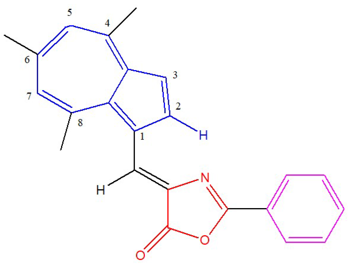
Advanced Materials Based on Azulenyl-Phenyloxazolone

by
Alina-Giorgiana Brotea
1,
Ovidiu-Teodor Matica
1,
Cornelia Musina (Borsaru)
1,
Mihaela Cristea
2,
Amalia Stefaniu
3,
Andreea-Madalina Pandele
4 and
Eleonora-Mihaela Ungureanu
1,*
1
Doctoral School of Chemical Engineering and Biotechnologies, Faculty of Chemical Engineering and Biotechnologies, University “Politehnica” of Bucharest, Gheorghe Polizu 1-7, Sector 1, 011061 Bucharest, Romania
2
Institute of Organic Chemistry “C. D. Nenitzescu” of the Romanian Academy, 71141 Bucharest, Romania
3
National Institute for Chemical-Pharmaceutical Research and Development, 112 Vitan Av., Sector 3, 031299 Bucharest, Romania
4
Advanced Polymer Materials Group, University Politehnica of Bucharest, Gh Polizu 1-7, 011061 Bucharest, Romania
*
Author to whom correspondence should be addressed.
Symmetry 2023, 15(2), 540; https://doi.org/10.3390/sym15020540
Submission received: 28 January 2023 / Revised: 10 February 2023 / Accepted: 13 February 2023 / Published: 17 February 2023
(This article belongs to the Section Chemistry: Symmetry/Asymmetry)

Abstract

:
Chemically modified electrodes (CMEs) based on 2-phenyl-4-((4,6,8-trimethylazulen-1-yl)methylene)oxazol-5(4H)-one (M) were obtained by irreversible electrooxidation of M in millimolar solutions in 0.1 M tetrabutylammonium perchlorate (TBAP) in acetonitrile. These CMEs were characterized by a ferrocene redox probe, electrochemical impedance spectroscopy (EIS), X-ray photon spectroscopy (XPS), and scanning electron microscopy (SEM). The influence of the preparation conditions (charge and potential) was examined. The CMEs were finally used for the analysis of synthetic samples of heavy metal (HM) ions. The paper highlights the importance of potential and electropolymerization charge on the film properties, with accent on recognition of HMs, in order to identify the best conditions for their detection in water. The observed findings are relevant for further design and development of advanced materials based on azulenyl-phenyloxazolone for the analysis of HMs in water.

1. Introduction

Oxazolones, also known as azlactones or oxazol-5(4H)-ones, are five-membered rings containing nitrogen and oxygen heteroatoms, demonstrated to be versatile scaffolds for various purposes in organic synthesis, due to the presence of pro-nucleophilic and electrophilic reactive sites in their structure [1] that basically consist of “masked” amino acids. Thus, oxazolones are considered important synthons for the synthesis of biologically active or peptidomimetic compounds. They can become the key monomer unit of various polymers and nanomaterials of biomedical uses [1,2,3,4] or an attractive heterocycle core of complex molecules with numerous biological or pharmaceutical applications involved in several organic transformations [5] (ring-opening reactions, cycloadditions to form new carbon–carbon and/or carbon–heteroatom bonds and to prepare various selective functionalized molecules, or conjugate additions, alkylation, allylation, arylation, acylation, etc.). For instance, in order to explore new clinical applications, new oxazolone derivatives have been reported as key scaffolds used to enhance the potential effectiveness of sulfonamides by preparing a novel series of 5(4H)-oxazolone-based-sulfonamides with antibacterial, antifungal, or anticancer activities [6]. Some oxazolone derivatives are reported as hypoglycemic agents [7], immunomodulators [8,9], and anti-inflammatory agents [10,11].
Azulene, a non-alternating aromatic hydrocarbon, exhibits low ionization energy, high electron mobility and a less symmetrical structure compared to naphthalene, its skeletal isomer. Due to its exceptional structure, with symmetrical electron distribution only with respect to the x-axis [12], azulene confers some special chemical and physical properties to the compounds in which it is inserted compared to compounds containing the naphthalene structure. Thus, azulene derivatives are used as building blocks for the generation of materials with valuable technical properties [13,14,15,16,17,18]. In particular, several organic compounds containing azulenyl group in their structure have been studied for potential medical applications [19,20].
The good electron-donating capability of azulene [21] motivated the investigation of push-pull compounds containing this moiety linked directly to an electron acceptor (Scheme 1, formula A) or via a conjugated bridge (Scheme 1, formula B) [22,23,24,25]. Thus, a great number of molecules with varying properties can be synthesized, taking into account the nature of the X=Y bridge and the wide variety of azulene donor groups and electron acceptor groups (Ac). Considering this, our main research focus was directed toward the synthesis and characterization of new molecules belonging to the entire series of compounds of the general formula B with specific properties. Recently, priority has been given to the substituted double bond (III) azulenes [26] to prepare 1-vinylazulenes with different substituents at the C=C double bond.
The presence of the azulen-1-yl moiety, which is capable of undergoing anodic polymerization, and of a functional group or system with a high affinity toward the cations determines the higher electron density for this second group. As a result, the affinity toward cations increases, i.e., the push-pull structures could be used to build modified electrodes with complexation properties. Of great research interest in the electrochemistry application field is the investigation of such organic push-pull systems due to their important technical properties, such as nonlinear optical (NLO) responses, electrochemical behavior, or coloring properties. Several polyazulenes were prepared as potential host molecules [27,28]. They were investigated by different measurements (UV-vis-NIR, EPR, SEM, CV) to find ways to enhance their special properties (conductivity, electronic switching or antioxidant character). These characteristics make them valuable for numerous applications in the technical field, as materials with NLO properties [29,30] or as potential ligands for metal ion detection [31].
Following the promising results from the newly synthesized azulenyl-phenyloxazolones [32,33] and their physicochemical analysis, we expanded our research to other compounds of the same class. This paper presents the characterization of 2-phenyl-4-85 ((4,6,8-trimethylazulen-1-yl)methylene)oxazol-5(4H)-one (M) from the class of azulen-1-ylmethylene-2-phenyloxazol-5(4H). The electrochemical properties of this compound have been determined together with polymerization attempts on the electrodes surface in order to obtain modified electrodes as metal sensors. A few other similar structures are being studied. In this paper, the electrochemical characteristics of M are initially described. The M′ structure (Figure 1) contains a part of oxazolone (in red) substituted with 2-phenyl (in magenta) and is connected to a 4,6,8-trimethylazulene moiety (in blue) through a C=C bond. The oxazolone ring is known for its HMs’ complexing properties [34]. The global structure of M corresponds to an extended conjugated system that generates an easily polymerizable monomer, whose electropolymerization has been attempted and successfully achieved.
Chemically modified electrodes based on M (M-CMEs) have been prepared by electropolymerization. They were examined by a ferrocene redox probe, EIS, XPS, and SEM using approaches similar to those recently published for other azulene derivatives [35]. Lastly, the obtained M-CMEs were tested for the detection of HM ions, and the influence of the electrochemical preparation conditions (charge and potential) has been examined in the analysis of synthetic samples of HMs.

2. Materials and Methods

M was synthesized as previously mentioned—by the condensation of azulene-1-carbaldehyde derivative with hippuric acid [32]. The main characteristics of M (characterization by elemental analysis, UV-Vis, 1H NMR, 13C-NMR, IR, and MS) are provided in the supplementary material.
Acetonitrile (CH3CN, Sigma Aldrich, electronic grade 99.999% trace metals) and tetrabutylammonium perchlorate (TBAP, Fluka, Munich, Germany, analytical purity ≥ 99.0%) were used without any other processing.
Salts containing the following metal cations: mercury (II) acetate (Fluka, Munich, Germany ≥ 98%), cadmium nitrate tetrahydrate (Fluka, Munich, Germany ≥ 98%), copper (II) acetate monohydrate (Fluka, Munich, Germany, ≥98%), and lead (II) nitrate (Fluka, Munich, Germany, ≥99.5%) were used. Firstly, 10−3 M stock solutions of HMs were prepared, followed by successive dilutions in order to obtain different concentrations of HMs.
All electrochemical determinations were carried out using an Autolab PGSTAT302N Autolab potentiostat connected to the cells with three electrodes. For electrochemical characterization and CMEs preparation, the working electrode (WE) was a glassy carbon (GC) disk (Metrohm, Herisau, Switzerland) of 3 mm diameter, the counter electrode (CE) was a platinum wire, and the reference electrode (RE) was Ag/10 mM AgNO3, 0.1 M TBAP/CH3CN. All potentials were referred to as the potential of the ferrocene/ferrocenium (Fc/Fc+) redox couple. For the electrochemical detection of HMs ions from aqueous solutions, a three-electrode cell (transfer cell) was used, these being: GC disks modified with M films for the working electrode, Ag/AgCl, 3 M KCl for the reference electrode, and the auxiliary electrode was a platinum wire. The electrochemical experiments for the characterization of M were performed under an argon atmosphere.
Cyclic voltammetry (CV) data were measured at scan rates of 0.05–0.5 V/s. The differential pulse voltammetry (DPV) data were measured at 0.01 V/s with a pulse height of 0.025 V and a step time of 0.2 s. Rotation rates between 500 and 1500 rpm were chosen to perform the rotating disk electrode voltammetry (RDE) measurements at 0.01 V/s.
Chemically modified electrodes (CMEs) were prepared from millimolar solutions of M in 0.1 M TBAP/CH3CN by scanning or controlled potential electrolysis (CPE). Then, each modified electrode (M-CME) was washed with acetonitrile and introduced in 0.1 M acetate aqueous buffer solution (pH = 4.5), where it was equilibrated and overoxidized using working procedures as previously mentioned [36,37]. The resultant electrodes were immersed under continuous stirring in synthetic solutions of HMs ions for 15 min. Then, the electrodes were withdrawn and rinsed with deionized water, then immersed in a cell containing 0.1 M acetate buffer solution (pH = 4.5). Here, they were polarized for 3 min at −1.0 V, and then their DPV data between −1.0 and +0.6 were registered.
EIS experiments were carried out using an Autolab potentiostat/galvanostat 302N (Ecochemie, Utrecht, The Netherlands) with a FRA2 impedance module on the frequency ranging from 100 kHz to 50 MHz by applying a potential with an amplitude of 10 mV over the dDC equilibrium potential (OCP). EIS measurements (star arrangement of WE, RE, and CE) were made in 0.1 M TBAP/CH3CN solution containing Fc (5 mM). Nyquist plots are employed to present the impedance data.
All electrochemical experiments were conducted at 25 °C.
SEM measurements were performed using Thermo Scientific model Apreo S equipment with a low acceleration voltage (2.5 kV and 5 kV) to avoid damaging the sample.
A Thermo Scientific K-Alpha spectrometer operating with monochromatic Al Kα X-rays (1486.6 eV) at a 90° take-off angle was used to achieve the XPS analysis. Survey and high-resolution spectra were recorded at 200 eV and 20 eV, respectively. A mixed Gaussian Lorentzian function was used for the deconvolution of core-level spectra after performing a Shirley background subtraction.

3. Results

3.1. Electrochemical Characterization of M

CV, DPV, and RDE oxidation and reduction curves were initially recorded on the freshly cleaned GC electrode in 0.1 M TBAP, CH3CN supporting electrolyte (SE). These curves have been represented by dashed lines. Then, M was added to SE, and its electrochemical behavior in millimolar solutions of decreasing concentrations was examined by CV, DPV and RDE methods. The anodic and cathodic peaks highlighted by DPV in these solutions were denoted in the order in which they appear in the DPV voltammograms starting from the equilibrium potential, and they were taken as reference. For a better comparison of anodic and cathodic current values, the cathodic currents were shown as absolute values.

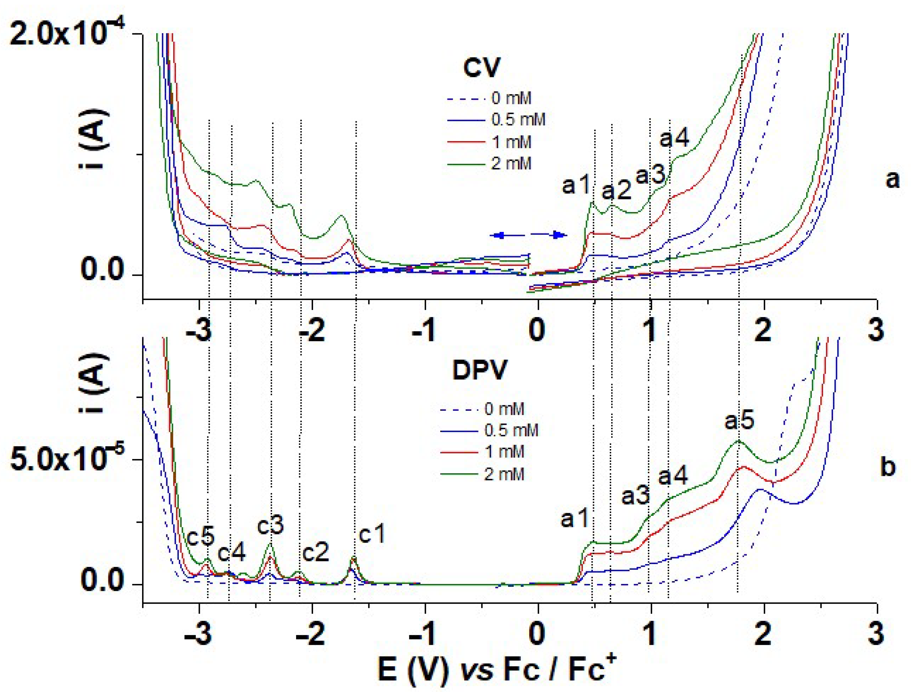
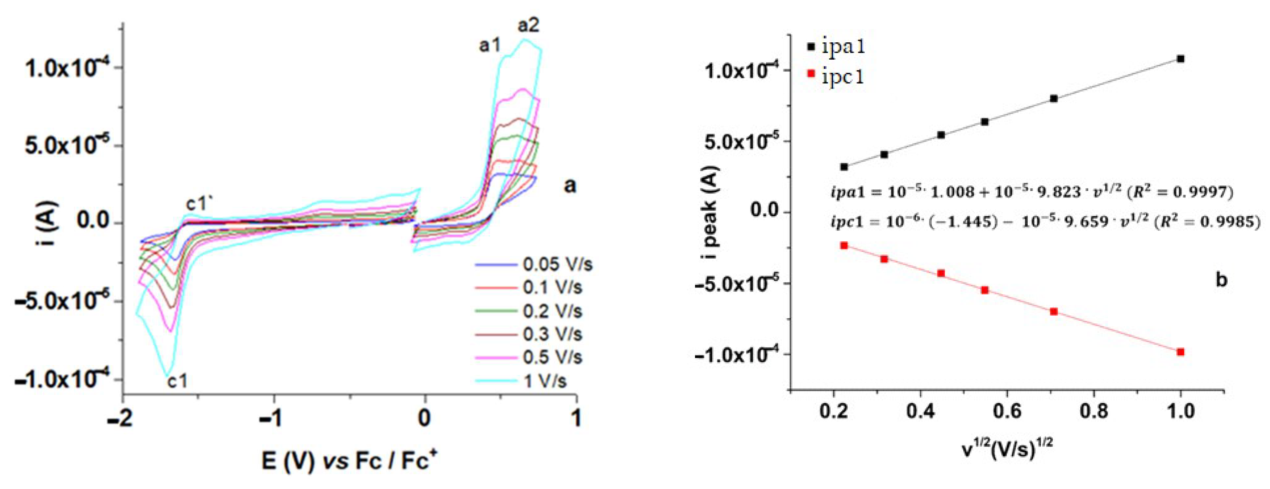
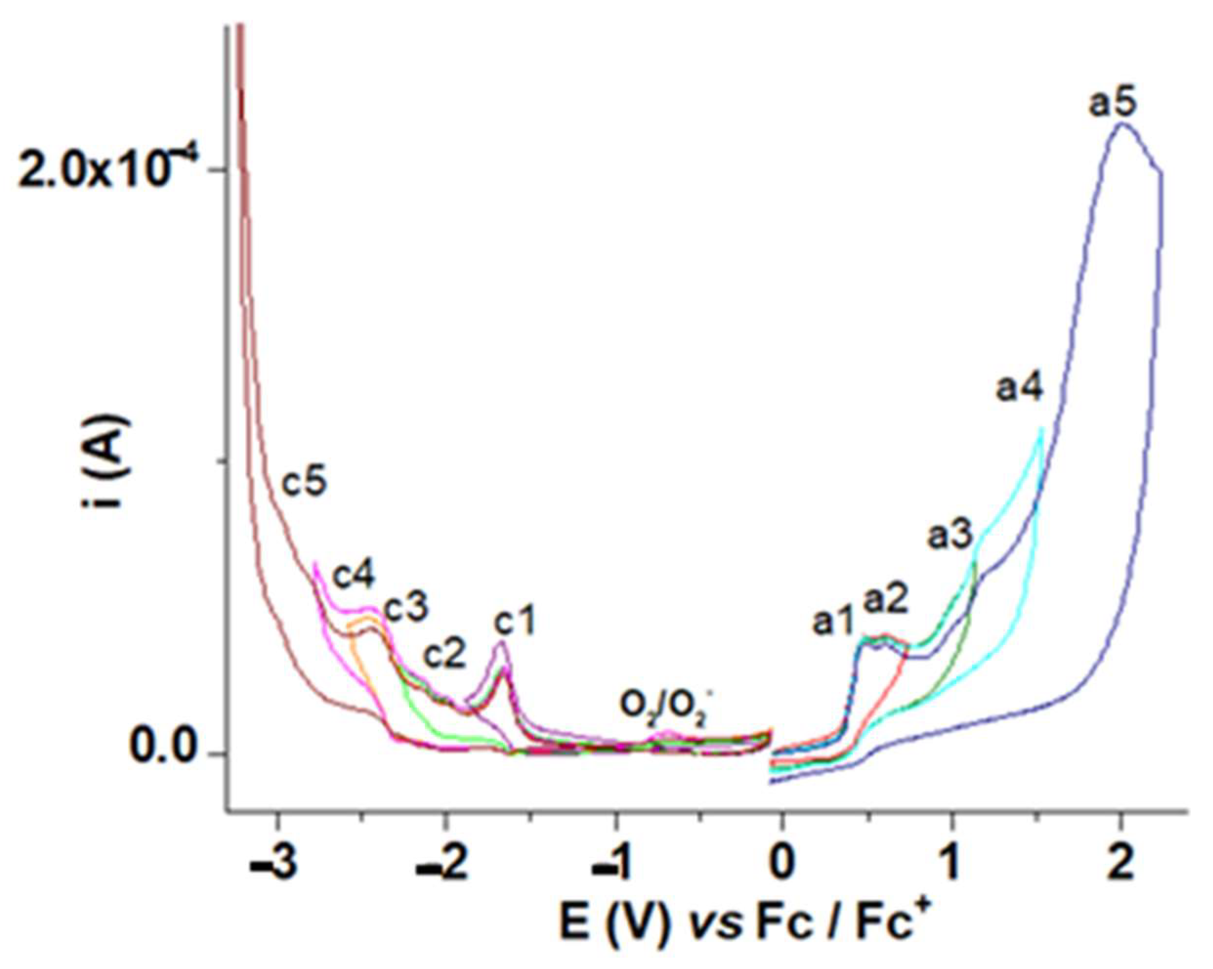
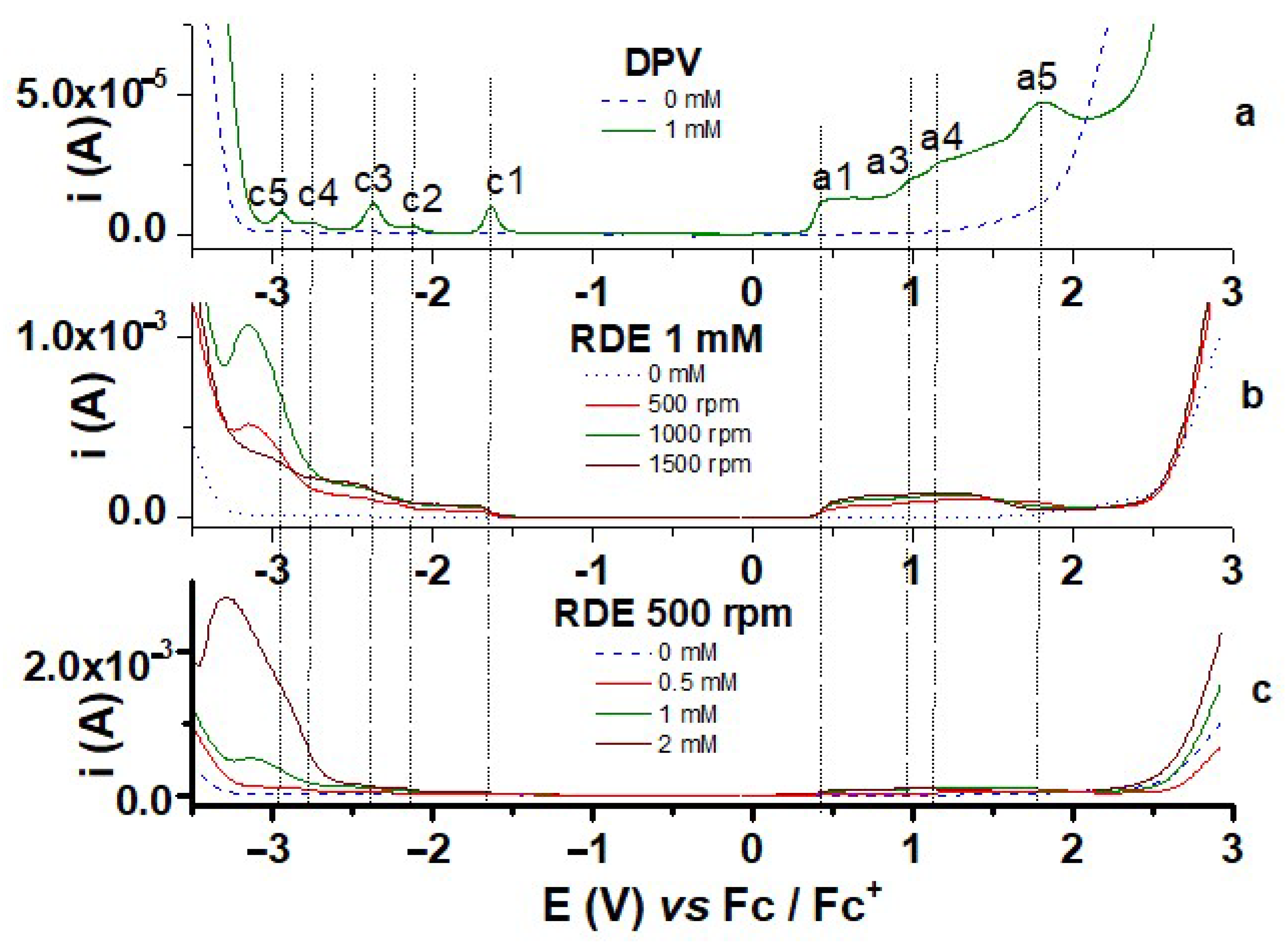
3.1.1. Characterization by CV and DPV

Characterization of M by CV at different concentrations of M (Figure 2), different scan rates (Figure 3), and scan domains (Figure 4) was performed. Five anodic (a1–a5) and five cathodic (c1–c5) peaks were evidenced in the anodic and cathodic scans, respectively, by DPV for different concentrations of M between 0 and 2 mM (Figure 2). To compare their peak potentials, which are given in Table 1, CV curves are shown in parallel with those obtained by DPV.

3.1.2. Characterization by RDE

Figure 5 illustrates in parallel the DPV (a) and RDE (b and c) curves obtained for [M] = 1 mM at different rotation rates of the rotating disk electrode (Figure 5b) and at different concentrations of M at a rotation rate of 500 rpm (Figure 5c). The half-wave RDE potential values (E1/2) that could be evaluated are summarized in Table 1.

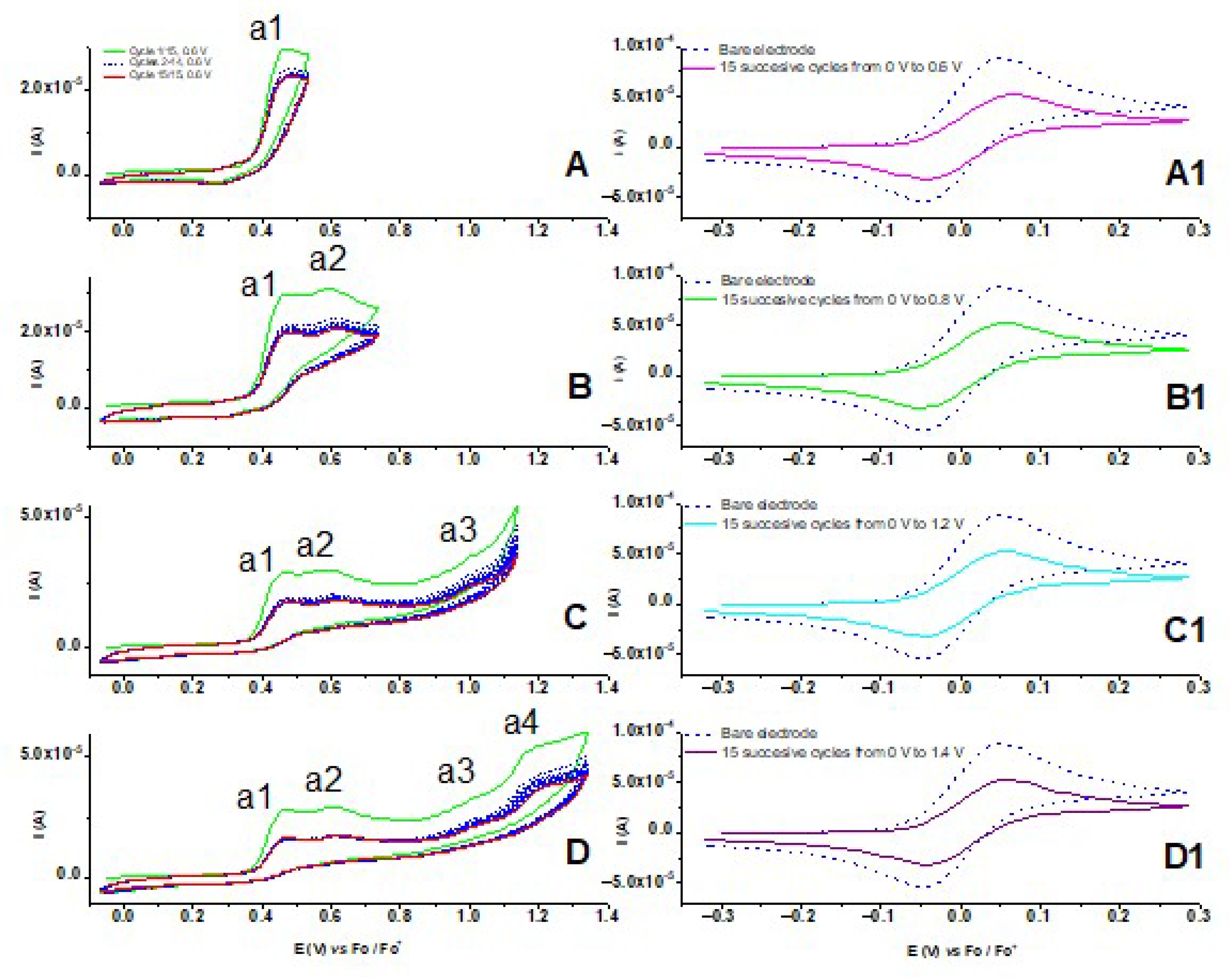
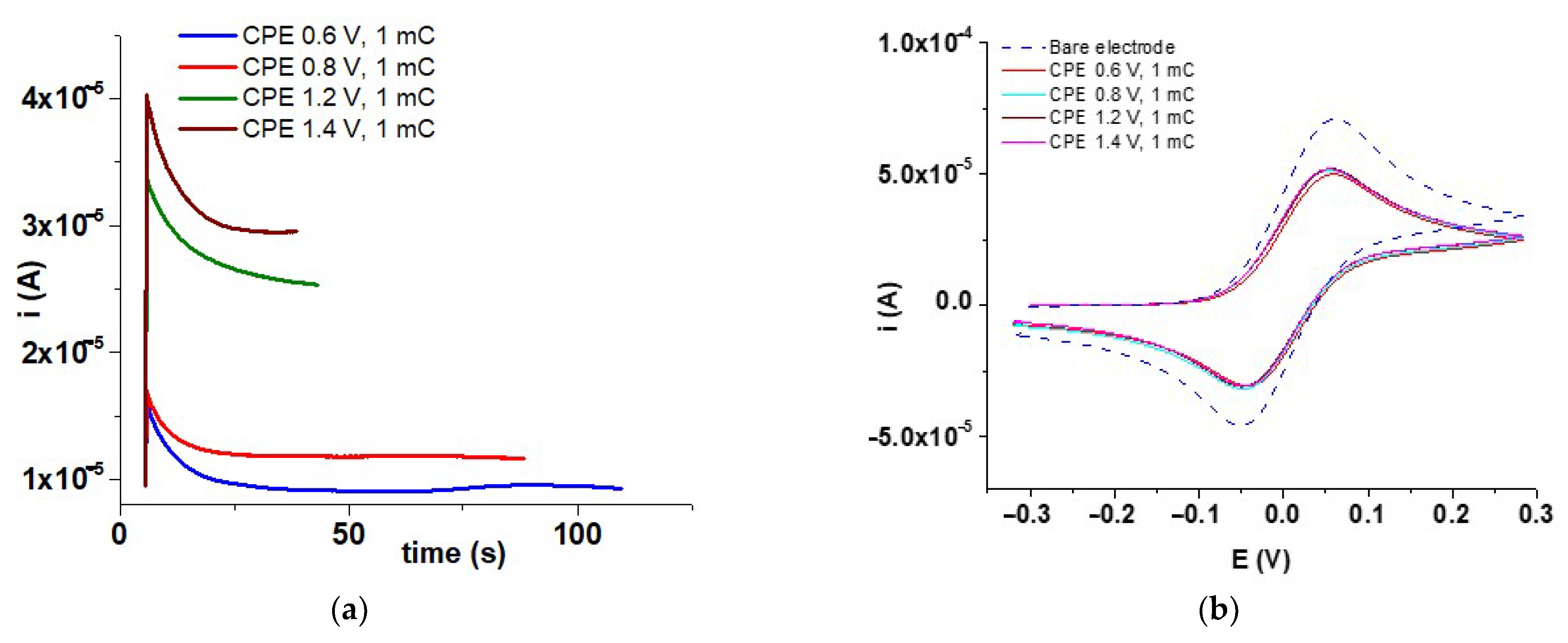
3.2. Preparation of the Modified Electrodes

Preparation of the modified electrodes was performed by electropolymerization at the potentials established by the voltammetric measurements in millimolar solutions of M in the supporting electrolyte (0.1 M TBAP/CH3CN) either by scanning or by CPE. The electrochemical immobilization of M on GC electrode was achieved at anodic potentials in the domain of (a1–a4) processes.
The different preparation conditions of M-CMEs are shown in Table 2, where the investigations are collected to evidence the films’ formation by electrochemical oxidation: Fc redox probe, chronoamperometry, EIS, SEM, XPS, analysis of HMs, and the reproducibility test for HMs analysis, which are discussed below.

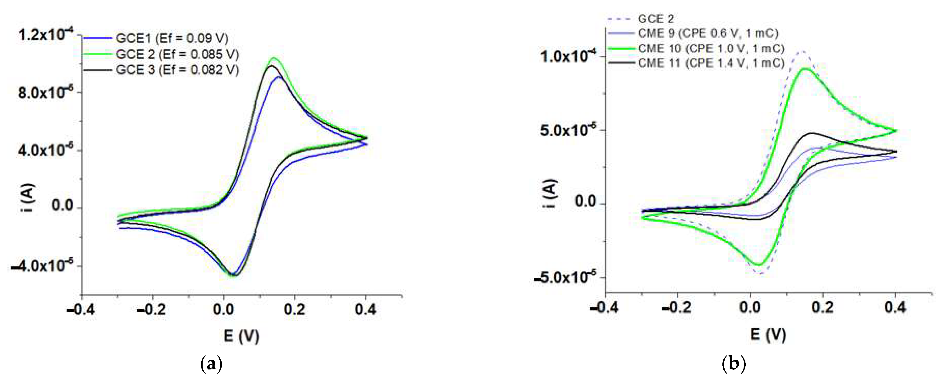
3.3. Evidence for M Films Formation by Fc Redox Probe

Evidence related to the formation of M-CMEs was obtained after transferring the modified electrodes (rinsed with acetonitrile after preparation) in ferrocene solutions in the supporting electrolyte without M. The CV curves for ferrocene obtained on M-CMEs were compared with those obtained on the bare electrode. The main characteristics (anodic and cathodic peak potentials and currents, formal potential, and potential difference between the anodic and cathodic peaks) were examined and are presented in Figure 6 and Figure 7, Table 3 and Table S1.
Figure 6 shows on the left side the evolution of the CV curves during the preparation of M films by scanning. M-CMEs were obtained in 2 mM solution of M in 0.1 M TBAP/CH3CN by scanning on different potential ranges in the domain of processes a1–a4. The right side of Figure 6 shows the corresponding CV curves after the transfer of M-CMEs in Fc solution, respectively, compared to the Fc signal on the bare electrode. The main characteristics of Fc in CV curves include the potential of Fc/Fc+ anodic (Epa) and cathodic (Epc) peak, the difference between Epa and Epc (ΔEp), and the formal potential (Ef) on M-CMEs, which are collected in Table S1.
The formation of M films on the GC electrode by CPE was also highlighted by the Fc redox probe. Currents during the film formation were recorded by chronoamperometry. In Figure 7a, several chronoamperograms obtained during CPE preparation at different potentials using the same electrical charge (1 mC) are exemplified. On the corresponding modified electrodes transferred into ferrocene solution, the CV curves of Figure 7b are obtained. Table 3 collects some characteristics of the Fc/Fc+ system resulting from CV curves for CMEs obtained at different potentials and those of the bare electrode. Figure S1 shows the CV curves at different scan rates on the modified electrodes, and the insets show the linear variations of Fc/Fc+ anodic (ipa) and cathodic (ipc) peak currents. The slopes of these lines vs. the square root of the scan rate are provided in their insets and are mentioned in the caption of Figure S1. Figure S2 shows the corresponding variations of the peak potentials (Epa and Epc) with the logarithm of the scan rate for the Fc/Fc+ redox system on the CMEs obtained at different potentials. The slopes of the obtained lines are given in each Figure and are mentioned in the caption of Figure S2.

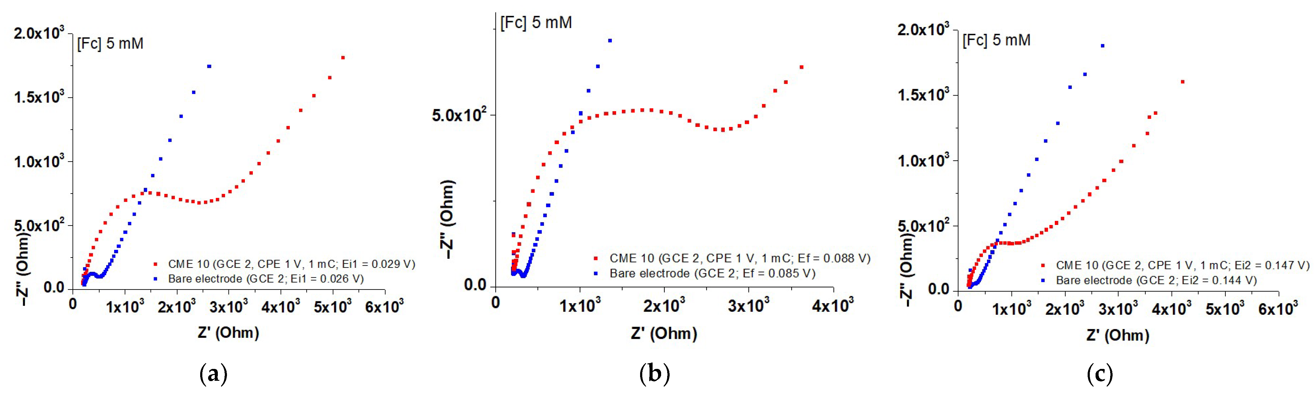
3.4. Characterization of M-CMEs by EIS

The EIS study was performed on CMEs in Fc solution (5 mM) in 0.1 M TBAP/CH3CN after their investigation by the Fc redox probe conducted in the same Fc solution.
Figure 8 shows the CV curves in Fc solution obtained on the unmodified (Figure 8a) and modified (Figure 8b) electrodes obtained at different potentials (highlighted by CV, DPV and RDE): 0.6 V (around process a1), 1 V (around peak potential a2) and at 1.4 V (after process a3). The resulting CMEs (CME 9, CME 10 and CME 11) were tested by EIS (Table 4). Impedance studies of the modified electrodes were then performed in the same Fc (5 mM) solution in 0.1 M TBAP/CH3CN. The experiments were performed at equilibrium potential (Eeq) and at the imposed potentials (Ei1, Ei2) given in Table 4. Figure 9 shows as an example of EIS curves obtained on CME 10 prepared at the potential of 1 V, and on the GC electrode on which the film was deposited. These curves show two types of variations (one hemispherical and one linear). From their intersection point, the value of the resistance to the charge transfer on the uncovered GC electrode (RGC) and on the film-modified (RMGC) electrodes were estimated (Table 5).
From the difference between RMGC and RGC (Rct = ΔR = RMGC − RGC), the charge transfer resistance through the film (Rct) was estimated for each M-CME film. The Rct values were evaluated for each potential (E) value applied in EIS (Table 5). The EIS curves on each uncovered electrode (GCE 1, GCE 2, GCE 3), and on the corresponding electrodes covered with films are shown in Figures S3 and S4.

3.5. Characterization of M-CMEs by SEM

SEM measurements were performed at different magnifications on M-CMEs prepared at potentials close to processes a1, a2 and a3 (at 0.6 V, 1 V and 1.4 V vs. RE) at constant electropolymerization charge of 14 mC/ cm2, and different electropolymerization charges (14–84 mC/cm2) at 0.6 V. The SEM images obtained under different conditions are given in Figures S5–S10.

3.6. Characterization of M-CMEs by XPS

Table 6 shows the plots of the C1s XPS core-level spectra for M-CMEs prepared at 1.4 V, 1 V, 0.6 V at 1 mC, and at different electropolymerization charges at 0.6 V. The ratio of C-C/C-O and C-C/O-C=O for these M-CMEs resulted from the variations in the surface chemistry observed in the C1s core-level spectra, as summarized in Table 7.

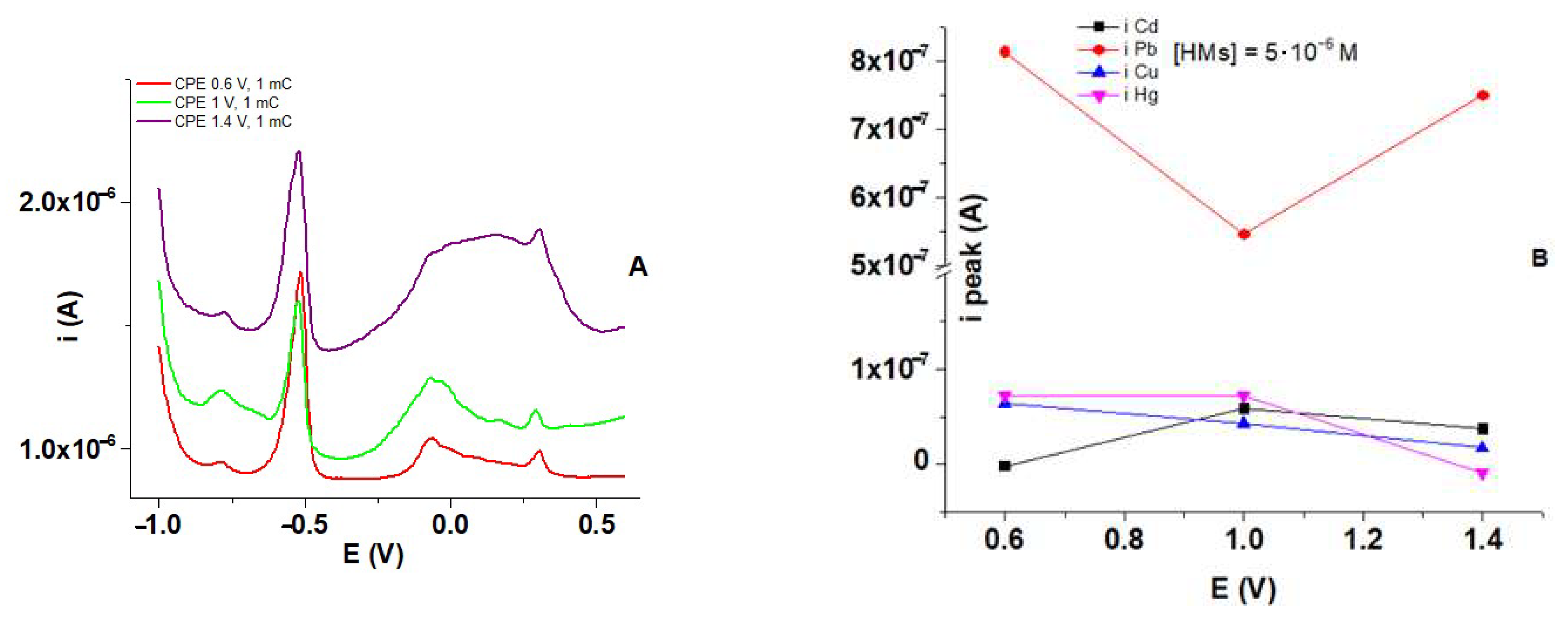
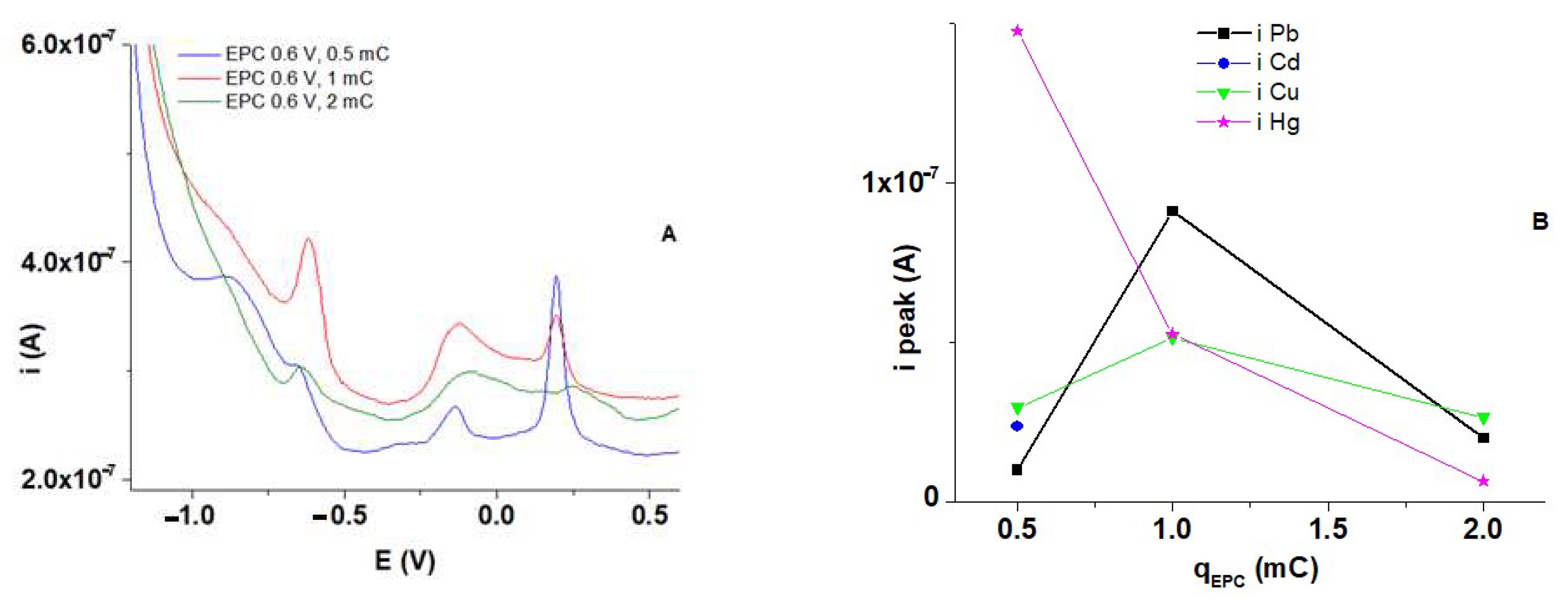
3.7. HMs Recognition Experiments Using polyM Films

For the HM ion-recognition experiments, M-CMEs were obtained by CPE at different potentials and electrical charges (Table 2). The CPE preparation method offers easy and rigorous control of potential and charge during electropolymerization. The anodic stripping method applied to the CMEs obtained by CPE at different potentials led to reproducible CMEs (Figure S11). This feature is very important in all quantitative applications, such as the analysis of HMs, especially for obtaining the calibration curve.
Then, each modified electrode (M-CME) was washed with acetonitrile and introduced in 0.1 M acetate aqueous buffer solution (pH = 4.5) where it was equilibrated (15 cycles between −0.9 V and 0.6 V) and overoxidized (15 cycles between –0.2 V and 1.85 V) using the procedures previously described [38]. They were then introduced into synthetic aqueous solutions containing a mixture of HMs ions at 5∙10−6 M HM concentrations for each ion and kept under magnetic stirring for 15 min; after that, they were placed in fresh acetate aqueous buffer solution (pH 4.5) and polarized for 3 min at –1.0 V (to reduce accumulated cations), and finally subjected to an anodic sweep using the DPV method (as in the examples shown in Figure 10A and Figure 11A).
Figure 10A shows the DPV curves obtained on CMEs prepared at different potentials. The DPV stripping peak currents were plotted against the electropolymerization potential for each investigated ion in the accumulation solution (Figure 10B), resulting in peaks for all the investigation cations at −0.8 V, −0.57 V, −0.1 V, and −0.22 V for Cd, Pb, Cu, Hg, respectively, but with different height.
From the tested potentials for CPE (0.6 V, 1 V, and 1.4 V), the value of 0.6 V corresponds to the potential of higher response for Pb (II). This potential was further considered for the synthesis of M-CMEs using different electrical charges to optimize the preparation conditions of these CMEs. At this potential, films of different thicknesses were prepared (Table 2) and tested in a solution containing a mixture of HM with concentrations of 5∙10−6 M for each of the investigated cations. Several stripping curves obtained are shown in Figure 11A. Figure 11B shows the plots of the peak currents for each cation as a function of the thickness of the prepared film.

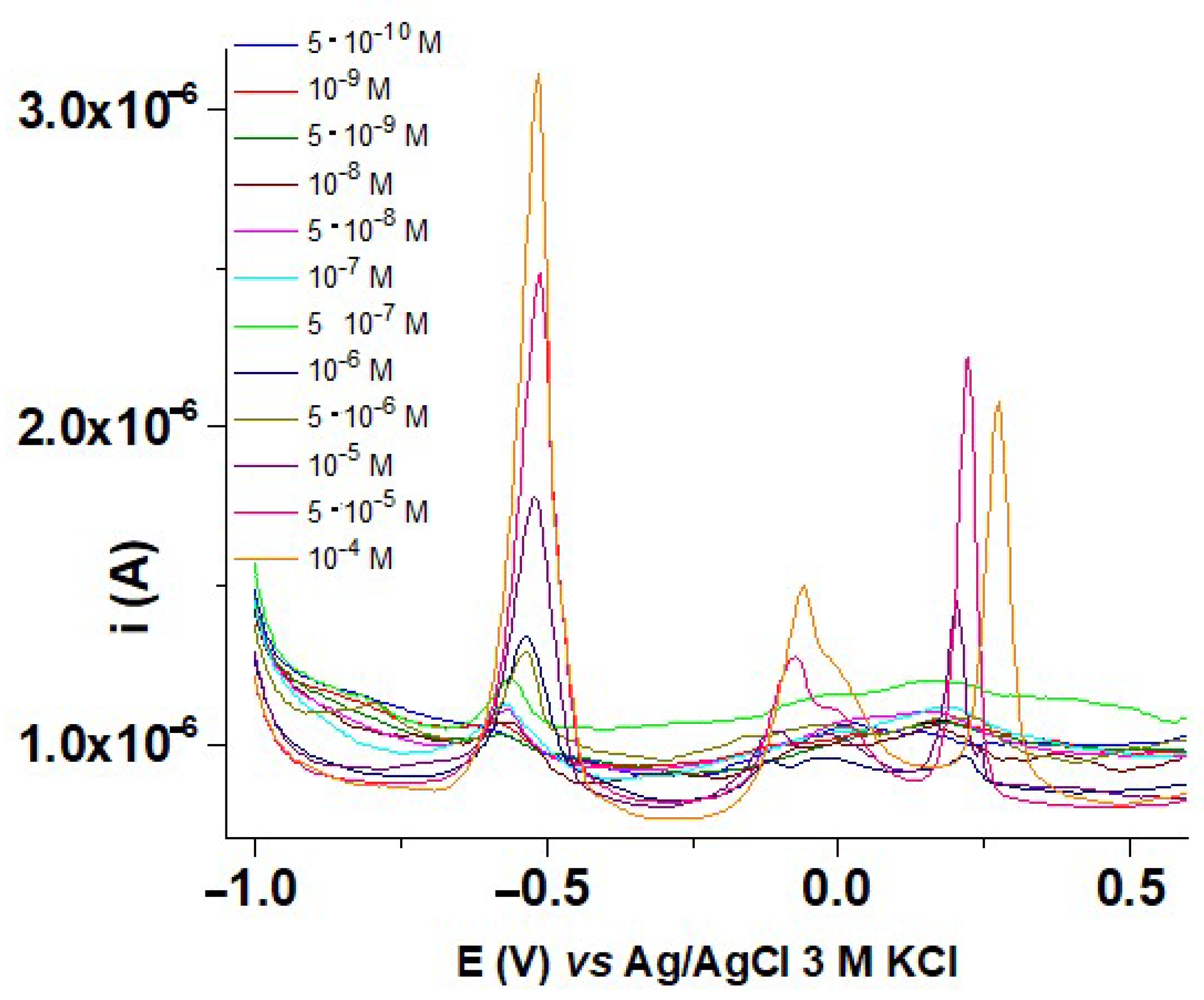
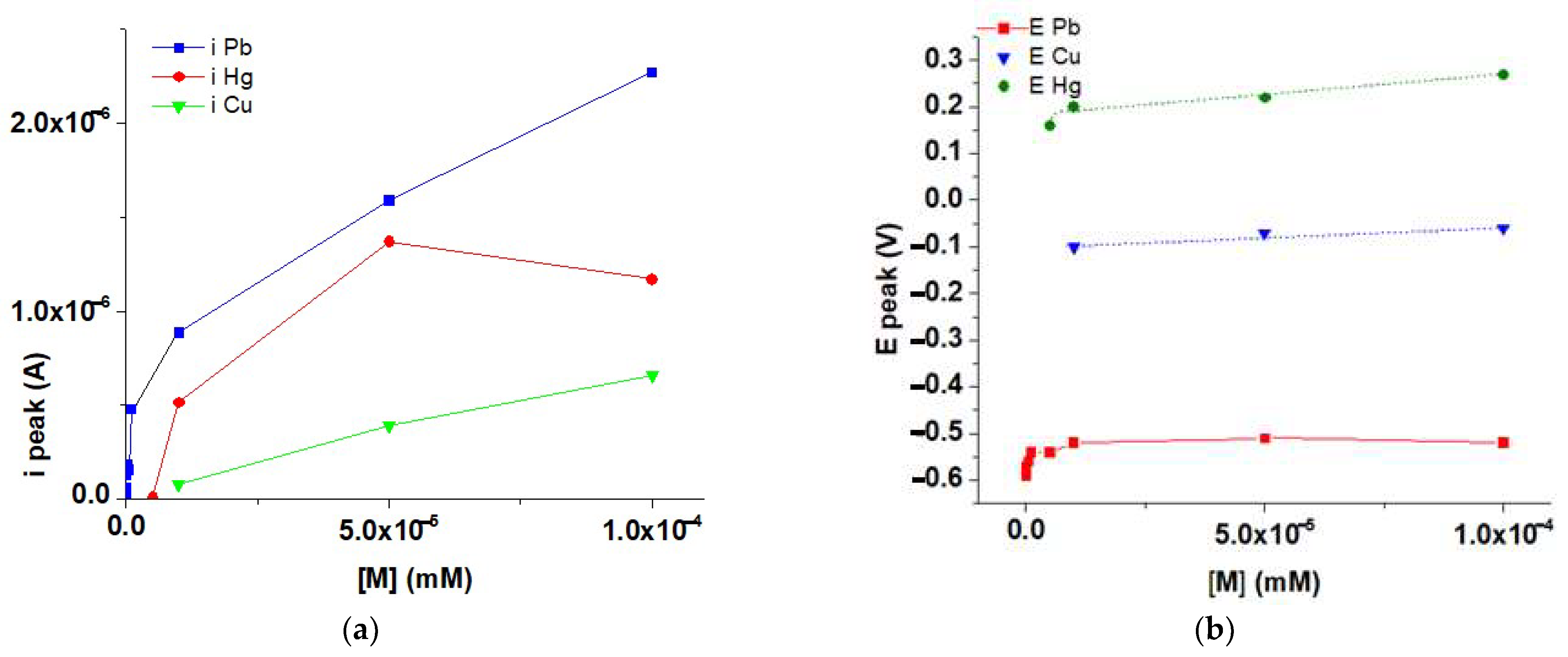
3.8. Influence of HMs Ions Concentrations on DPV Response

To obtain the calibration curve for HM analysis on M-CMEs prepared at the potential of 0.6 V and using an electropolymerization charge of 1 mC, the modified electrodes were immersed in accumulation solutions containing HM mixtures of Cd, Pb, Cu and Hg ions with equal concentrations varying between 5 × 10⁻¹⁰ M and 10−4 M (Figure 12). The dependencies of DPV peak currents and potentials on metal ion concentrations are shown in Figure 13a and Figure 13b, respectively. More data were collected in Table S2.

4. Discussion

Evidence for M Films Formation

In the electrochemical studies of the M ligand, five oxidation processes (a1–a5) and five reduction processes (c1–c5) were noticed, which intensified with increasing M concentration (Figure 2). The cathodic peak potentials in CV and DPV are properly correlated (the peak potential in DPV is close in value to the half-peak potential in CV). From the detailed analysis of the curves obtained by the three voltammetric methods used, some conclusions can be drawn regarding the processes that appear in the oxidation and reduction scans (Table 1).
From the CV, DPV and RDE curves (Figure 2 and Figure 5), the potentials of the processes highlighted by these voltammetric methods were obtained (Table 1). The analysis of these curves also allowed for some particularities of the processes to be highlighted, as listed in Table 1. Thus, the CV and RDE currents in the anodic domain are higher than those in the cathodic domain, while the situation is reversed in the RDE (Figure 5). These features can be explained by the difference in complexity of the processes involved (oxidation, reduction and the formation of films). It is noteworthy that the anodic peak a2 appears in CV for all ligand concentrations but does not appear in DPV (Table 1). This may be due to the formation of films at this potential by anodic oxidation, which were certified and further analyzed in this paper. In addition, the potential of the a5 DPV peak is shifted to more negative values when the M concentration increases. This displacement can be attributed to the value of this potential close to that at which oxidation processes occur in the supporting electrolyte (the formation of oxides, which occurs due to the inherent presence of traces of water in the organic electrolyte).
As can be seen from Figure 3a, the currents for the first anodic peak (a1) and the first cathodic peak (c1) increase with the scan rate. For peaks a1 and c1, the correlations are linear with the square root of the scan rate (Figure 3b), showing that these processes are diffusion controlled. From the slopes of these linear dependencies (0.98 × 10⁻⁴ and −0.97 × 10⁻⁴ A·V−1/2·s1/2, respectively), a 1:1 ratio can be estimated between the numbers of electrons that participate in the first oxidation/reduction process. The anodic peak a1 has a small counter peak in the reverse scan (and was considered quasireversible in Table 1), while a2 has no counterpart in the return scan and represents an irreversible process (Figure 3a and Figure 4). The peak c1 has a corresponding peak (c1′) and was considered quasireversible (the potential difference between peaks c1 and c1′ is 0.127 V, being slightly higher than 0.100 V recorded for the reversible Fc/Fc+ system in the used experimental assembly). This last feature is confirmed by the CVs over different scan domains in Figure 4. From this Figure 4, it can be estimated that the processes c2 and c3 are also quasireversible. All other peaks highlighted at higher potentials (positive or negative) appear as irreversible (Table 1).
The comparison of the RDE and DPV methods (as exemplified in Figure 5a, Figure 5b, and Figure 5c, respectively) shows that the currents of the anodic processes are much lower in relation to the cathodic ones. This evident asymmetry is due to film formation occurring more readily at anodic potentials. These films are insulators and block the surface of the electrode, resulting in decreased currents.
From the RDE curves in Figure 5b, which were recorded for a concentration of 1 mM, increasing the electrode rotation rate does not greatly influence the oxidation currents, which are small in absolute value. There is a slight increase in the RDE wave from ~0.5 V (which confirms the assignment of quasireversible to correspond, which is likely due to the film formation of a radical-cation from M. This is similar behavior to the previous experiments for benzylidenerhodanine [38] and rhodanine [39]). The formation of cations in azulene is the most likely reaction that can take place at the first oxidation point, because the azulene system is the most easily oxidizable. For potentials more positive than +1.5 V the situation is reversed. An isosbestic point for the current is observed at ~1.5 V. At this potential, there is a change of the electrochemical process to the one started at the potential of the a2 peak. In the cathodic potential range, the RDE currents are higher than the anodic ones and increase when the electrode rotation rate increases from 500 to 1000 rpm, decreasing from 1000 at 1500 rpm.
Figure 5c shows an obvious asymmetry of the curves obtained in the anodic and cathodic scans from the RDE. The concentration of M is important especially for cathodic processes, while for anodic ones it is relevant only at potentials more positive than +2 V, in the field of solvent oxidation processes. The curves are consistent with those in Figure 5b (for different rotation rates). The shape of the RDE curves changes in the cathodic range with respect to M concentration from that of a wave (at 0.5 mM and 1 mM) to that of a peak (at 2 mM), as expected, given the role of monomer concentration in a polymerization process. Film formation is favored at a concentration of M equal to 2 mM compared to 1 mM and 0.5 mM. Covering the electrode with film leads to a peak-shaped RDE curve. This is consistent with the formation of insulating films, as the films obtained by electropolymerization of M proved to be and as will be shown below. The latter explanation agrees with the decrease in RDE cathodic currents from 1000 to 1500 rpm, which can be seen in Figure 5b.
The RDE study for the cathodic processes showed a significant increase of the currents with the concentration of M. The peak-shaped of the RDE curves at potentials more negative than −3 V (Figure 5c) shows that at these potentials a cathodic polymerization process takes place, as also observed on other azulene substrates [37].
Film formation by the electropolymerization of M was evidenced by a ferrocene redox probe. When testing M-CMEs, obtained either by scanning or CPE in ferrocene solution in the supporting electrolyte (0.1 M TBAP/CH3CN), the CV curves obtained on M-CMEs (as those presented on the right side of Figure 6) show much lower currents for Fc compared to those recorded on the bare electrode, but the potential at which ferrocene appears is practically the same (Table S1 and Table 3, respectively), indicating the formation of some isolating thin films.
The EIS curves bring valuable information on M-CMEs related to the films’ formation evidence as in the case of other compounds [40]. For instance, the EIS curves for M-CME shown in Figure 9 support the presence of polymer films deposited on the electrode surface at this potential (1 V corresponds to processes occurring mainly in a2 peak). Similar behavior was noticed for films prepared at 0.6 and 1.4 V. The semicircular region of the Nyquist plot at higher frequencies corresponds to a limiting electron transfer process. From its diameter, one can estimate the electron transfer resistance (Rct), which controls the electron transfer kinetics at the electrode interface. From the Nyquist plots for those unmodified (Figure S3) and modified with polymer film (Figure S4), the GC electrodes obtained by CPE at 1.0 V on GCE 2 show that the imaginary part of the impedance (-Z″) is larger for the modified GC electrode, confirming the coating of the electrode with film by electropolymerization. This result agrees with the results obtained by CV (Figure 8).
The modified electrodes investigated by EIS were initially analyzed by the redox probe method in ferrocene. Figures S1 and S2 show the CV curves at different scan rates obtained during the characterization in Fc/SE for CME 9, CME 10 and CME 11, all obtained by CPE, but at different potentials (0.6 V, 1.0 V and 1.4 V, respectively). Figure S1 shows the slopes of the linear dependencies of the peak currents on the square root of the scanning rate for each electrode: 6.031 × 10⁻⁵ A·(V/s)−1/2 (CME 9); 8.634 × 10⁻⁵ A·(V/s)−1/2 (CME 10); 2.988 × 10⁻⁵ A·(V/s)−1/2 (CME 11). From these slopes, the active surface area of CMEs (A) was calculated for each film using the Randles–Sevcik Equation (1)
ip = 2.69 · 105 · n3/2 · A·D1/2 · C · v1/2
In (1), ip is the peak current (A), n is the number of transferred electrons (n = 1), A is the geometric surface area (cm2), D is the diffusion coefficient of the redox probe (2.62∙10−9 cm2/s [41,42,43]), C is the redox probe concentration (mol/cm3), and v is scan rate of the potential (V/s). The values obtained for A are 0.072 cm2, 0.103 cm2, and 0.036 cm2, respectively, indicating film surfaces for these CMEs of the same order of magnitude as the geometric area of the electrode (S = 0.071 cm2). These values for A depend on the applied electropolymerization potential.
During the characterization of the modified electrodes by EIS, the curves obtained on M-CME were compared with those obtained on unmodified GC electrodes (Table 2). From the curves shown in Figure 9, Figures S3 and S4, the resistance to electric charge transfer through the deposited film (RMGC) was evaluated (Table 5). Comparison of EIS curves in the presence and absence of films at different potentials of the EIS study shows that the resistance to electric charge transfer through the film (RMGC) increases compared to that on the bare electrode (RGC), as can be seen from Table 5 where the RMGC values are higher than the corresponding RGC values. The difference between the RMGC and RGC values was assessed as the resistance to charge transfer through the films (ΔR). From Table 5, it was observed the increase of ΔR was due to the film formation (ΔR = RMGC − RGC > 0). This increase, highlighted on the modified electrodes prepared by CPE, has positive values and depends on the potential applied in the synthesis (0.6 V, 1.0 V, 1.4 V), as well as on the potential applied to the EIS (Table 5).
M-CMEs were analyzed by SEM. As in the case of other azulenes [37], the influence of the potential on the morphology of the films prepared at these potentials for different charges of electropolymerization was examined. The films obtained at potentials of 0.6 V, 1 V, and 1.4 V were tested using the same load of 14 mC/cm2 and at 0.6 V at different electropolymerization charges, including 14 mC/cm2, 28 mC/cm2, 56 mC/cm2 and 84 mC/cm2, respectively. The surface morphology of the prepared samples was examined to see the influence of each parameter on the evaluated property. Table 6 shows the deconvolution curves resulting from XPS depending on two variables (electric charge and potential applied during electropolymerization). SEM images for M-CMEs (Figures S5–S10) show a relatively uniform surface arrangement of the polymer matrix. Some clusters are observed on the surface that deviate from the planarity of the sample. Also, the surface shows some mechanical defects (scratches) due to the preliminary cleaning of the electrode before the preparation of the sample.
M-CMEs were analyzed by XPS. Variations in surface chemistry are clearly visible in C1s core-level spectra, which were also used to describe the electrode surface after each modification [44]. The C1s core-level spectra allowed a closer examination of the chemical state of element C, as shown in Table 6, and was deconvoluted in three components [45] at around 284 eV, 286 eV and 288 eV. These peaks could be clearly noticed in all samples, except for sample P1. In sample P1, the C 1s peak was deconvoluted into two components, at 284.6 eV (C-C/C=C) and 285.7 eV (C-O). The carbon atoms involved in the C-C/C=C bond and originating from the conjugated honeycomb network of azulene were identified by the strong peak displayed at approximately 284.8 eV and were presented throughout the sample. The C-O and O-C=O bond at 286.2 eV and 288.9 eV originated from a methyl oxazolone film deposited on a carbon electrode.
Since the aim of XPS experiments was to see how the variation of the two parameters (potential and electrical charge during electropolymerization) affects the chemistry of the electrode surface, the ratio between C-C/C-O and C-C/O-C=O for samples P2 -P6 has also been calculated for comparison. From Table 7, it can be seen a decrease in the C-C/C-O ratio from 5.68 in the case of the P2 sample to about 2.40 in the case of the P3-P6 samples and an increase in the C-C/O-C=O ratio from 8.45 to about 12 in the case of samples P3-P5. On the basis of these XPS values, it can be said that the variation of the electropolymerization potential from +1 V in P2 to 0.6 V in P3 leads to significant changes in the surface state. In case of samples P3–P5, the variation in the electropolymerization charge does not affect the surface chemistry of the films deposited on the carbon electrodes (the C-C/C-O and C-C/O-C=O ratios have small variations). From the survey curves, the ratio between the percentage of C and O (C/O) was calculated, which indicates the oxidation of the polymer with the increase of the potential applied to the electrodes.
Taking into account the AT values, it is observed that the component from 288.9 eV is practically constant for the films of different thicknesses obtained at a potential of 0.6 V at which no overoxidation of the polymer. Polymerization is slower at this potential. However, the images obtained in SEM show that the film was not very homogeneous for the different values of electrical charges, even if the polymerization was done at 0.6 V, which explains these small variations of the SEM signals. Comparing the influence of the potential, it can be seen that the best coverage is obtained at a potential of 1 V, at which the most regular structure appears. At the potential higher than 1.4 V, a polymerization can take place that leads to gaps in the polymer due to the rapid development of the polymer given the favorable potential, or there is an impairment of the signal due to the carbon substrate because the films are thin and non-conductive. The results for the samples obtained at different potentials can be correlated with the electrochemical calculations for the active surface of the polymer, which shows an increase from the potential of 0.6 V to 1 V followed by a decrease towards the value of 1.4 V. The choice of the optimal polymerization potential will depend on the purpose for which these modified electrodes will be used.
For HMs ion analysis, M-CMEs were obtained by CPE, a method that provides easy and rigorous control of potential and charge during electropolymerization (Table 2). After preparation, equilibration and superoxidation following anodic stripping procedures highlighted in our laboratory, DPV curves were recorded between −1.0 V and 0.6 V. They show stripping peaks for all studied ions. This demonstrates that these ions were complexed into the electrogenerated films. For CMEs obtained at 0.6 V and 1 mC, peaks for Cd, Pb, Cu, and Hg dissolution were observed at potentials of approximately −0.80, −0.54, −0.08, and 0.23 V, respectively, which varies slightly with the concentration of metal ions in the analyzed mixture (Figure 13). However, the most important signal appears for the Pb ion.
The influence of the electric potential and charge used in the CPE on the DPV response was examined for each of the HM cations that were analyzed.
The influence of the electric potential used in the CPE on the DPV response shows that of the tested potentials the value of 0.6 V of the potential corresponds to the highest response for Pb (II). This potential is located near the a1 peak, reported in the electrochemical study of monomer M, and corresponds to the formation of a more porous film than that prepared at the potentials of the other anodic peaks of M. A potential of 0.6 V was considered for the synthesis of M-CME in the process of optimizing the preparation conditions of these CMEs. Films of different thicknesses were prepared and tested at this potential. Their stripping curves show an optimal response for an electrical charge of 1 mC for Pb and Cu, while the thinner film of 0.5 mC is favorable for Hg ion.
For the calibration curves for HMs analysis on M-CMEs, accumulation solutions were used between 5 × 10⁻¹⁰ M and 10−4 M, which showed better results for Pb among the other investigated ions. Linear dependencies for Pb were obtained in the range of concentration between 5 × 10⁻¹⁰ M and 5 × 10⁻⁵ M. From the dependences of peak DPV currents for M-CMEs prepared at 0.6 V, 1 mC on metal ion concentrations, the detection limits for each HM ion were estimated, namely: [Cd] = 5 × 10⁻⁶ M; [Pb] = 5 × 10⁻¹⁰ M; [Cu] = 10−5 M; [Hg] = 5 × 10⁻⁶ M.

5. Conclusions

The experimental study using electrochemistry and EIS, SEM, and XPS reports on the influence of the main parameters that can be optimized (the potential and electric charge for film formation) for the properties of the films obtained by the electropolymerization of 2-phenyl-4-((4,6,8-trimethylazulen-1-yl)methylene)oxazol-5(4H)-one (M). All of the methods confirmed the formation of films. M-CMEs were used for the recognition of Cd, Pb, Cu and Hg ions. For the HM ion recognition experiments, the best results were obtained for Pb(II).
This study is important for those working to create advanced materials based on azulenyl-phenyloxazolone and for further applications, including developing new detection materials based on CME for the analysis of HMs in water. Studies on similar ligands for CMEs are ongoing.

Supplementary Materials

The following supporting information can be downloaded at: https://www.mdpi.com/article/10.3390/sym15020540/s1, Figure S1. Study of the scan rate influence on ferrocene peak currents recorded on M-CMEs prepared on: GCE 1 (CME 9, 0.6 V, 1 mC) (a); GCE 2 (CME 10, 1 V, 1 mC) (b); GCE 3 (CME 11, 1.4 V, 1 mC). Insets: linear dependences of the peak currents on the square root of the scan rate, for each electrode with a slope of 6.031 × 10⁻⁵ A·(V/s)−1/2 (CME 9); 8.634 × 10⁻⁵ A·(V/s)−1/2 (CME 10); 2.988 × 10⁻⁵ A·(V/s)−1/2 (CME 11); Figure S2. Variation of the peak potential of ferrocene in 5 mM solution in 0.1 M TBAP/CH3CN (Epa) vs log v (v in V/s for CME 9 (a), CME 10 (b), CME 11 (c) with slopes of: 0.021 V (CME 9); 0.081 V (CME 10); 0.022 V (CME 11), respectively, for Epa and of 0.012 V (CME 9); 0.003 V (CME 10); 0.020 V (CME 11), respectively, for Epc; Figure S3. Impedance curves in Fc 5 mM for the bare electrode GCE 2 (1 V, 1 mC) at equilibrium potential (Eeq) ~0.085 V (blue), and at imposed potentials (Ei1, Ei2) ~0.026 V (black) and ~0.144 V (green), respectively; Figure S4. Impedance curves recorded in Fc 5 mM at different potentials on: CME 9 (obtained at 0.6 V) at Ei1~0.037 V (black), Eeq~0.096 V (blue), Ei2~0.155 V (green); CME 10 (obtained at 1 V) at Ei1~0.029 V (black), Eeq~0.088 V (blue), Ei2~0.147 V (green); CME 11 (obtained at 1.4 V) at Ei1~0.031 V (black), Eeq~0.090 V (blue), Ei2~0.149 V (green); Figure S5. SEM images of the polymer surfaces obtained by CPE at 1.4 V, 4 mC (14 mC/cm2) (CME 12) at two magnifications: ×300, 5 kV (a) and ×105, 2.5 kV (b); Figure S6. SEM images of the polymer surfaces obtained by CPE at 1 V, 4 mC (14 mC/cm2) (CME 13) at two magnifications: ×300, 5 kV (a) and ×105, 2.5 kV (b); Figure S7. SEM images of the polymer surfaces obtained by CPE at 0.6 V, 4 mC (14 mC/cm2) (CME 14) at two magnifications: ×300, 5 kV (a) and ×105, 2.5 kV (b); Figure S8. SEM images of the polymer surfaces obtained by CPE at 0.6 V, 8 mC (28 mC/cm2) (CME 15) at two magnifications: ×300, 5 kV (a) and ×105, 2.5 kV (b); Figure S9. SEM images of the polymer surfaces obtained by CPE at 0.6 V, 16 mC (56 mC/cm2) (CME 16) at two magnifications: ×300, 5 kV (a) and ×105, 2.5 kV (b); Figure S10. SEM images of the polymer surfaces obtained by CPE at 0.6 V, 24 mC (84 mC/cm2) (CME 17) at two magnifications: ×300, 5 kV (a) and ×105, 2.5 kV (b); Figure S11. DPV curves (0.01 V/s−1) recorded on M-CMEs, prepared by CPE at 1 mC and different potentials: 0.6 V (a), 1 V (b), and 1.4 V (c) corresponding to 5∙10−6 M concentration of each mixed metal; Table S1. Potentials vs. Fc/Fc+ (Epa, Epc) and currents (ipa, ipc) of Fc/Fc+ anodic and cathodic peaks in 3 mM Fc solution in 0.1 M TBAP/CH3CN for GC bare electrode and for the modified electrodes prepared by scanning in solution with [M] = 2 mM in 15 successive cycles on different anodic potential domains; Table S2. Main characteristics of the DPV peaks recorded on M-CMEs (obtained by CPE at 0.6 V and 1 mC) for different concentrations of mixed metals in the aqueous accumulation solution.

Author Contributions

Conceptualization, E.-M.U.; methodology, E.-M.U.; software, A.S.; validation, E.-M.U. and M.C.; formal analysis, A.-G.B., O.-T.M. and C.M.B.; investigation, A.-G.B., C.M.B., O.-T.M. and A.-M.P.; resources, M.C.; data curation, A.S., A.-M.P. and E.-M.U.; writing—original draft preparation, A.-G.B.; writing—review and editing, E.-M.U. and A.S.; visualization, A.S.; supervision, A.-M.P., O.-T.M. and E.-M.U.; project administration, E.-M.U. All authors have read and agreed to the published version of the manuscript.

Funding

This research received no external funding.

Institutional Review Board Statement

Not applicable.

Informed Consent Statement

Not applicable.

Data Availability Statement

The data that support the findings of this work are available upon request from the corresponding author.

Acknowledgments

This work was supported by a grant from the Ministry of Research, Innovation and Digitization, CNCS-UEFISCDI, project number PN-III-P1-1.1-TE-2021-1163, within PNCDI III.

Conflicts of Interest

The authors declare no conflict of interest.

References

  1. De Castro, P.P.; Carpanez, A.G.; Amarante, G.W. Azlactone Reaction Developments. Chem. Eur. J. 2016, 22, 10294–10318. [Google Scholar] [CrossRef] [PubMed]
  2. Zayas-Gonzalez, Y.M.; Ortiz, B.J.; Lynn, D.M. Layer-by-Layer Assembly of Amine-Reactive Multilayers Using an Azlactone-Functionalized Polymer and Small-Molecule Diamine Linkers. Biomacromolecules 2017, 18, 1499–1508. [Google Scholar] [CrossRef] [PubMed] [Green Version]
  3. Wang, X.; Davis, J.L.; Aden, B.M.; Lokitz, B.S.; Kilbey, S.M. Versatile Synthesis of Amine-Reactive Microgels by Self-Assembly of Azlactone-Containing Block Copolymers. Macromolecules 2018, 51, 3691–3701. [Google Scholar] [CrossRef]
  4. Chauveau, C.; Vanbiervliet, E.; Fouquay, S.; Michaud, G.; Simon, F.; Carpentier, J.-F.; Guillaume, S.M. Azlactone Telechelic Polyolefins as Precursors to Polyamides: A Combination of Metathesis Polymerization and Polyaddition Reactions. Macromolecules 2018, 51, 8084–8099. [Google Scholar] [CrossRef]
  5. Marra, I.F.S.; de Castro, P.P.; Amarante, G.W. Recent Advances in Azlactone Transformations. Eur. J. Org. Chem. 2019, 2019, 5830–5855. [Google Scholar] [CrossRef]
  6. Almalki, A.J.; Ibrahim, T.S.; Taher, E.S.; Mohamed, M.F.A.; Youns, M.; Hegazy, W.A.H.; Al-Mahmoudy, A.M.M. Synthesis, Antimicrobial, Anti-Virulence and Anticancer Evaluation of New 5(4H)-Oxazolone-Based Sulfonamides. Molecules 2022, 27, 671. [Google Scholar] [CrossRef]
  7. Mariappan, G.; Saha, B.P.; Datta, S.; Kumar, D.; Haldar, P.K. Design, synthesis and antidiabetic evaluation of oxazolone derivatives. J. Chem. Sci. 2011, 123, 335–341. [Google Scholar] [CrossRef] [Green Version]
  8. Rodrigues, C.A.B.; Martinho, J.M.G.; Afonso, C.A.M. Synthesis of a Biologically Active Oxazol-5-(4H)-one via an Erlenmeyer–Plöchl Reaction. J. Chem. Educ. 2015, 92, 1543–1546. [Google Scholar] [CrossRef]
  9. Mesaik, M.A.; Rahat, S.; Khan, K.M.; Zia, U.; Choudhary, M.I.; Murad, S.; Ismail, Z.; Attaur, R.; Ahmad, A. Synthesis and immunomodulatory properties of selected oxazolone derivatives. Bioorg. Med. Chem. 2004, 12, 2049–2057. [Google Scholar] [CrossRef]
  10. Tandel, R.; Mammen, D. Synthesis and Study of Some Compounds Containing Oxazolone Ring, Showing Biological Activity. Indian J. Chem. 2008, 47, 932–937. [Google Scholar] [CrossRef]
  11. Hassanein, H.H.; Khalifa, M.M.; El-Samaloty, O.N.; El-Rahim, M.A.; Taha, R.A.; Magda; Ismail, M.F. Synthesis and biological evaluation of novel imidazolone derivatives as potential COX-2 inhibitors. Arch. Pharmacal. Res. 2008, 31, 562. [Google Scholar] [CrossRef] [PubMed]
  12. Razus, A.C. Azulene Moiety as Electron Reservoir in Positively Charged Systems; A Short Survey. Symmetry 2021, 13, 526. [Google Scholar] [CrossRef]
  13. Ghazvini Zadeh, E.H.; Tang, S.; Woodward, A.W.; Liu, T.; Bondar, M.V.; Belfield, K.D. Chromophoric Materials Derived from a Natural Azulene: Syntheses, Halochromism and One-Photon and Two-Photon Microlithography. J. Mater. Chem. C 2015, 3, 8495. [Google Scholar] [CrossRef]
  14. Koch, M.; Blacque, O.; Venkatesan, K.; Mater, J. Impact of 2,6-connectivity in azulene: Optical properties and stimuli responsive behavior. J. Mater. Chem. C 2013, 1, 7400. [Google Scholar] [CrossRef] [Green Version]
  15. Ito, S.; Morita, N. Creation of Stabilized Electrochromic Materials by Taking Advantage of Azulene Skeletons. Eur. J. Org. Chem. 2009, 27, 4567–4579. [Google Scholar] [CrossRef]
  16. Tsurui, K.; Murai, M.; Ku, S.-Y.; Hawker, C.J.; Robb, M.J. Modulating the Properties of Azulene-Containing Polymers through Controlled Incorporation of Regioisomers. Adv. Funct. Mater. 2014, 24, 7338–7347. [Google Scholar] [CrossRef] [Green Version]
  17. Wang, X.; Kok-Peng Ng, J.; Jia, P.; Lin, T.; Mui Cho, C.; Xu, J.; Lu, X.; He, C. Synthesis, Electronic, and Emission Spectroscopy, and Electrochromic Characterization of Azulene-Fluorene Conjugated Oligomers and Polymers. Macromolecules 2009, 42, 5534–5544. [Google Scholar] [CrossRef]
  18. Amir, E.; Amir, R.J.; Campos, L.M.; Hawker, C.J. Stimuli-Responsive Azulene-Based Conjugated Oligomers with Polyaniline-like Properties. J. Am. Chem. Soc. 2011, 133, 10046–10049. [Google Scholar] [CrossRef]
  19. Bakun, P.; Czarczynska-Goslinska, B.; Goslinski, T.; Lijewski, S. In vitro and in vivo biological activities of azulene derivatives with potential applications in medicine. Med. Chem. Res. 2021, 30, 834–846. [Google Scholar] [CrossRef]
  20. Vasile (Corbei), A.-A.; Stefaniu, A.; Pintilie, L.; Stanciu, G.; Ungureanu, E.-M. In Silico characterization and preliminary anticancer assessment of some 1,3,4-Thiadiazoles. UPB Sci. Bull. B 2021, 83, 3–12. [Google Scholar]
  21. Zeller, K.P. Houben Weyl, Methoden der Organischen Chemie. Thieme Stuttgart 1985, 5/2c, 127. [Google Scholar]
  22. McDonald, R.N.; Stewart, W.S. Nonbenzenoid Aromatic Systems. I. Synthesis of 1-Vinylazulene and Certain Substituted 1-Vinylazulenes. J. Org. Chem. 1965, 30, 270. [Google Scholar] [CrossRef]
  23. Hafner, K. Neuere Ergebnisse der Azulen-Chemie. Angew. Chem. 1958, 70, 419. [Google Scholar] [CrossRef]
  24. Hunig, S.; Ort, B. Mehrstufige reversible Redoxsysteme, XXXVII. Biazulenyle und ω, ω′-Biazulenylpolyene: Synthesen und spektroskopische Eigenschaften. Liebigs Ann. Chem. 1984, 12, 1905–1935. [Google Scholar] [CrossRef]
  25. Briquet, A.A.S.; Hansen, H.J. New Results in the Synthesis of Styrylazulene Derivatives: Application of the ‘Anil synthesis’ to the preparation of azulenes substituted with styryl groups at the seven-membered ring. Helv. Chim. Acta 1994, 77, 1921–1939. [Google Scholar] [CrossRef]
  26. Razus, A.C.; Birzan, L. Synthesis of azulenic compounds with a homo-or hetero-atomic double bond at position 1. Arkivoc 2018, part VI, 1–56. [Google Scholar] [CrossRef]
  27. Wang, F.; Lai, Y.-H.; Han, M.-Y. Stimuli-Responsive Conjugated Copolymers Having Electro-Active Azulene and Bithiophene Units in the Polymer Skeleton: Effect of Protonation and p-Doping on Conducting Properties. Macromolecules 2004, 37, 3222–3230. [Google Scholar] [CrossRef]
  28. Lete, C.; Esteban, B.M.; Kvarnström, C.; Razus, A.C.; Ivaska, A. Electrosynthesis and characterization of poly(2-[(E)-2-azulen-1-ylvinyl] thiophene) using polyazulene as model compound. Electrochim. Acta 2007, 52, 6476–6483. [Google Scholar] [CrossRef]
  29. Iftime, G.; Lacroix, P.G.; Nakatani, K.; Razus, A.C. Push-pull azulene-based chromophores with nonlinear optical properties. Tetrahedron Lett. 1998, 39, 6853. [Google Scholar] [CrossRef]
  30. Asato, A.E.; Liu, R.S.H.; Rao, V.P.; Cai, Y.M. Azulene-containing donor-acceptor compounds as second-order nonlinear chromophores. Tetrahedron Lett. 1996, 37, 419–422. [Google Scholar] [CrossRef]
  31. Birzan, L.; Cristea, M.; Draghici, C.C.; Tecuceanu, V.; Maganu, M.; Hanganu, A.; Arnold, G.-L.; Ungureanu, E.-M.; Razus, A.C. 1-vinylazulenes–potential host molecules in ligands for metal ion detectors. Tetrahedron 2016, 72, 2316. [Google Scholar] [CrossRef]
  32. Cristea, M.; Bîrzan, L.; Dumitrascu, F.; Enache, C.; Tecuceanu, V.; Hanganu, A.; Draghici, C.; Deleanu, C.; Nicolescu, A.; Maganu, M.; et al. 1-Vinylazulenes with Oxazolonic Ring-Potential Ligands for Metal Ion Detectors; Synthesis and Products Properties. Symmetry 2021, 13, 1209. [Google Scholar] [CrossRef]
  33. Sharma, N.; Banerjee, J.; Shrestha, N.; Chaudhury, D. A review on oxazolone, it’ s method of synthesis and biological activity. Eur. J. Biomed. Pharm. Sci. 2015, 2, 964–987. Available online: https://www.researchgate.net/publication/280882247 (accessed on 26 January 2023).
  34. Garcia-Sanz, C.; Andreu, A.; de las Rivas, B.; Jimenez, A.I.; Pop, A.; Silvestru, C.; Palomo, J.M. Pd-Oxazolone complexes conjugated to an engineered enzyme: Improving fluorescence and catalytic properties. Org. Biomol. Chem. 2021, 19, 2773–2783. [Google Scholar] [CrossRef] [PubMed]
  35. Anastasoaie, V.; Omocea, C.; Enache, L.-B.; Anicai, L.; Ungureanu, E.-M.; van Staden, J.F.; Enachescu, M. Surface Characterization of New Azulene-Based CMEs for Sensing. Symmetry 2021, 13, 2292. [Google Scholar] [CrossRef]
  36. Enache, L.-B.; Anastasoaie, V.; Lete, C.; Brotea, A.G.; Matica, O.-T.; Amarandei, C.-A.; Brandel, J.; Ungureanu, E.-M.; Enachescu, M. Polyazulene-Based Materials for Heavy Metal Ion Detection. 3. (E)-5-((6-t-Butyl-4,8-dimethylazulen-1-yl) diazenyl)-1H-tetrazole-Based Modified Electrodes. Symmetry 2021, 13, 1642. [Google Scholar] [CrossRef]
  37. Păun, A.-M.; Matica, O.-T.; Anăstăsoaie, V.; Enache, L.-B.; Diacu, E.; Ungureanu, E.-M. Recognition of Heavy Metal Ions by Using E-5-((5-Isopropyl-3,8-Dimethylazulen-1-yl) Dyazenyl)-1H-Tetrazole Modified Electrodes. Symmetry 2021, 13, 644. [Google Scholar] [CrossRef]
  38. Matica, O.-T.; Brotea, A.G.; Ungureanu, E.M.; Stefaniu, A. Electrochemical and Spectral Studies on Benzylidenerhodanine for Sensor Development for Heavy Metals in Waters. Appl. Sci. 2022, 12, 2681. [Google Scholar] [CrossRef]
  39. Matica, O.-T.; Brotea, A.G.; Ungureanu, E.M.; Mandoc, L.R.; Birzan, L. Electrochemical and spectral studies of rhodanine in view of heavy metals determination. Electrochem. Sci. Adv. 2022, 1–11. [Google Scholar] [CrossRef]
  40. Buica, G.-O.; Maior, I.; Ungureanu, E.M.; Vaireanu, D.I.; Diacu, E.; Bucher, C.; Saint-Aman, E. Electrochemical Impedance Characterization of Poly (Pyrrole-EDTA Like) Modified Electrodes. Rev. Chim. 2009, 60, 1205–1209. [Google Scholar]
  41. Wang, Y.; Rogers, E.I.; Compton, R.G. The measurement of the diffusion coefficients of ferrocene and ferrocenium and their temperature dependence in acetonitrile using double potential step microdisk electrode chronoamperometry. J. Electroanal. Chem. 2010, 648, 15–19. [Google Scholar] [CrossRef]
  42. Morikita, T.; Yamamoto, T. Electrochemical determination of diffusion coefficient of π-conjugated polymers containing ferrocene unit. J. Organomet. Chem. 2001, 637–639, 809–812. [Google Scholar] [CrossRef]
  43. Ikeuchi, H.; Kanakubo, M. Diffusion Coefficients of Ferrocene and Ferricinium Ion in Tetraethylammonium Perchlorate Acetonitrile Solutions, as Determined by Chronoamperometry. Electrochemistry 2001, 69, 34–36. [Google Scholar] [CrossRef] [Green Version]
  44. Krishna, D.N.G.; Philip, J. Review on surface-characterization applications of X-ray photoelectron spectroscopy (XPS): Recent developments and challenges. Appl. Surf. Sci. Adv. 2022, 12, 100332. [Google Scholar] [CrossRef]
  45. Chiticaru, E.A.; Pilan, L.; Damian, C.-M.; Vasile, E.; Burns, J.S.; Ionită, M. Influence of Graphene Oxide Concentration when Fabricating an Electrochemical Biosensor for DNA Detection. Biosensors 2019, 9, 113. [Google Scholar] [CrossRef] [Green Version]
Scheme 1. Structures of push-pull compounds containing azulene moiety: azulenes (A) and 1-vinylazulenes (B).
Symmetry 15 00540 sch001
Figure 1. Structure of investigated compound 2-phenyl-4-((4,6,8-trimethylazulen-1-yl)methylene)oxazol-5(4H)-one (M).
Symmetry 15 00540 g001
Figure 2. CV (a) and DPV (b) curves for different concentrations of M in 0.1 M TBAP/CH3CN; the anodic peaks a1–a5 and the cathodic peaks c1–c5 are established by CV and DPV; all cathodic currents are shown in absolute values.
Symmetry 15 00540 g002
Figure 3. Anodic and cathodic CV curves at different scan rates for [M] = 1 mM in 0.1 M TBAP, CH3CN (a); linear dependencies of the currents for (a1) and (c1) peaks, respectively, on the square root of the scan rate (b).
Symmetry 15 00540 g003
Figure 4. Anodic and cathodic CV (0.1 V/s) curves for M (1 mM) in 0.1 M TBAP/ CH3CN on different scan domains (differently colored); all cathodic currents are shown in absolute values.
Symmetry 15 00540 g004
Figure 5. DPV (a) and RDE curves (b,c) on glassy carbon at different rotation rates (rpm) for [M] = 1 mM in 0.1 M TBAP/CH3CN (b) and, RDE curves at 500 rpm (c) at different concentrations in 0.1 M TBAP/ CH3CN; the cathodic currents are shown in absolute values.
Symmetry 15 00540 g005
Figure 6. Successive CVs (0.1 V/s, 15 cycles) in 2 mM solution of M in 0.1 M TBAP/ CH3CN performed with different anodic limit scan potentials (AD), increasing in the following order: (A) < (B) < (C) < (D), and the curves of the corresponding M-CMEs (A1D1) in ferrocene solution (1 mM in 0.1 M TBAP/CH3CN) with respect to those on the bare electrode (dashed lines).
Symmetry 15 00540 g006
Figure 7. Chronoamperograms during the preparation of M-CMEs in 1 mM solution of M in 0.1 M TBAP, CH3CN by CPE at different potentials (a); CV curves (0.1 V/s) after the transfer of M-CMEs in ferrocene solution (3 mM) in 0.1M TBAP/CH3CN—continuous lines vs. bare electrode—dashed line (b).
Symmetry 15 00540 g007
Figure 8. CV curves (0.1 V/ s) in Fc solution (5 mM) in 0.1 M TBAP/ CH3CN on bare electrodes GCE 1, GCE 2, GCE 3 having close formal potentials (a) and on M-CMEs prepared in different conditions vs. bare electrode GCE 2 (b) shown with a dashed line.
Symmetry 15 00540 g008
Figure 9. Nyquist impedance plots in Fc solution (5 mM) for CME 10 (red squares, prepared at 1 V, 1 mC) compared to the bare electrode (blue squares, GCE 2) recorded at the potential Ei1~0.026 V (a), Eeq~0.085 V (b), and Ei2~0.144 V (c).
Symmetry 15 00540 g009
Figure 10. DPV curves recorded on M-CMEs prepared by CPE using the electropolymerization charges of 1 mC at different potentials (A): 0.6 V (red), 1.0 V (green), and 1.4 V (purple) after accumulation in a solution of 5∙10−6 M concentrations of each metal; DPV peak currents dependencies on potential (B) for each investigated ion.
Symmetry 15 00540 g010
Figure 11. DPV curves recorded on M-CMEs prepared by CPE at 0.6 V and different charges: 0.5 mC (blue), 1.0 mC (red) and 2 mC (olive) after accumulation in a solution of 5 × 10⁻⁶ M concentrations of each metal (A); DPV peak currents dependencies on a charge of electropolymerization (B) for each investigated ion.
Symmetry 15 00540 g011
Figure 12. DPV curves (0.01 V/s−1) recorded on M-CMEs (obtained by CPE at 0.6 V and 1 mC) for different concentrations of mixed metals.
Symmetry 15 00540 g012
Figure 13. Dependencies of DPV peak current (a) and potential (b) on the metallic ion’s concentrations in the mixture for each investigated cation recorded on M-CMEs obtained by CPE at 0.6 V and using an electropolymerization charge of 1 mC.
Symmetry 15 00540 g013
Table 1. Potentials (V vs. Fc/Fc+) of the peaks evidenced in anodic (a) and cathodic (c) scans from CV and DPV curves, and the half-wave potential (E1/2) values for the corresponding waves from RDE curves and characteristics of the peaks recorded for M solutions (2 mM) in 0.1 M TBAP/CH3CN.
PeakMethodPeak Characteristics
CVDPVRDE (E1/2)
a10.4790.4840.431 (500 rpm)
0.441 (1000 rpm)
0.440 (1500 rpm)
Quasireversible
a20.657-0.630 (500 rpm)Irreversible
a31.1200.9811.070 (500 rpm)Irreversible
a41.2361.163-Irreversible
a5 1.777-Irreversible
c1−1.743−1.629−1.651 (500 rpm)
−1.651 (1000 rpm)
−1.650 (1500 rpm)
Quasireversible
c2−2.201−2.119−2.247 (500 rpm)Quasireversible
c3−2.496−2.371−2.412 (500 rpm)Quasireversible
c4-−2.763-Irreversible
c5-−2.926-Irreversible
Table 2. Conditions for the preparation of the modified electrodes by scanning (S) or controlled potential electrolysis (CPE) at different potentials (in M solutions of different concentrations [M] in 0.1 M TBAP, CH3CN), and their analysis.
Sample[M]
(mM)
PreparationElectrical Charge
(mC)
Electrical Charge Density
(mC/cm2)
Analysis
CME 12S * (0–0.6)--Fc redox probe *a
CME 22S * (0–0.8)--Fc redox probe *a
CME 32S * (0–1.2)--Fc redox probe *a
CME 42S * (0–1.4)--Fc redox probe *a
CME 5–5b2CPE at 0.6 V114Chrono *b, Fc redox probe *a
CME 6–6b2CPE at 0.8 V114Chrono *b, Fc redox probe *a
CME 7–7b2CPE at 1.2 V114Chrono *b, Fc redox probe *a
CME 8–8b2CPE at 1.4 V114Chrono *b, Fc redox probe *a
CME 9–9b2CPE at 0.6 V114Chrono *b, Fc redox probe *a, EIS
CME 10–10b2CPE at 1 V114Chrono *b, Fc redox probe *a, EIS
CME 11–11b2CPE at 1.4 V114Chrono *b, Fc redox probe *a, EIS
CME 121CPE at +1.4 V414Chrono *b, SEM, XPS
CME 131CPE at +1 V414Chrono *b, SEM, XPS
CME 141CPE at +0.6 V414Chrono *b, SEM, XPS
CME 151CPE at +0.6 V828Chrono *b, SEM, XPS
CME 161CPE at +0.6 V1656Chrono *b, SEM, XPS
CME 171CPE at +0.6 V2484Chrono *b, SEM, XPS
CME 18–18m2CPE at +0.6 V114Chrono *b, HMs *c, R *d
CME 19–19m2CPE at +1.0 V114Chrono *b, HMs *c, R *d
CME 20–20d2CPE at +1.4 V114Chrono *b, HMs *c, R *d
CME 21–21b2CPE at +0.6 V0.57Chrono *b, HMs *c, R *d
CME 22–22b2CPE at +0.6 V114Chrono *b, HMs *c, R *d
CME 23–23b2CPE at +0.6 V228Chrono *b, HMs *c, R *d
* Preparation by scanning (15 cycles) between the given potentials (in V) vs. RE; *a Transfer in Fc solution in 0.1 M TBAP/CH3CN; *b Chronoamperometry; *c Analysis of HMs solutions; *d Reproducibility test for HMs analysis.
Table 3. Potentials of Fc anodic (Epa) and cathodic (Epc) peaks in 3 mM Fc solution in 0.1 M TBAP/ CH3CN on the bare electrode and on the M-CMEs prepared by CPE for an electrical charge of 1 mC at different anodic potentials (ECPE) in solution with [M] = 2 mM.
Crt. Nr.ECPE (V)
(M-CME)
Epa
(V)
105·ipa
(A)
Epc
(V)
105·ipc
(A)
ΔEp *1
(mV)
Ef *2
(V)
1Bare electrode0.0617.141−0.049−4.5981100.055
20.6 (CME 5)0.0625.006−0.039−3.0981010.051
30.8 (CME 6)0.0525.159−0.049−3.2011010.051
41.2 (CME 7)0.0525.201−0.049−3.1091010.051
51.4 (CME 8)0.0525.201−0.049−3.0981010.051
*1 ΔEp = Epa − Epc; *2 Ef = (Epa + Epc)/2.
Table 4. EIS parameters (Eeq, Ei1, Ei2) for experiments carried out in Fc solution (5 mM) in 0.1 M TBAP/CH3CN on bare electrodes (GCE1–GCE3) and M-CMEs (CME 9–CME 11, obtained by CPE in the solution with [M] = 2 mM in 0.1 M TBAP, CH3CN at different potentials using a charge of 1 mC).
Nr. Crt.Modified ElectrodeCharacteristics of Film SynthesisEeq (V)Ei1 (V)Ei2 (V)
1GCE 1-0.0900.0310.149
2GCE 2-0.0850.0260.144
3GCE 3-0.0820.0230.141
4CME 9GCE 1, 0.6 V, 1 mC0.0960.0370.155
5CME 10GCE 2, 1 V, 1 mC0.0880.0290.147
6CME 11GCE 3, 1.4 V, 1 mC0.0900.0310.149
Table 5. Estimated values for Rct = ΔR for different values of EIS applied potential (E) obtained from the EIS curves recorded on bare GC (RGC) and film-coated (RMGC) electrodes prepared by CPE at different potentials.
Nr. Crt.Modified Electrode (Preparation Potential)E (V)10−3·RGC (Ω)10−3·RMGC (Ω)10−3·(ΔR) (Ω)
1CME 9 (0.6 V)Ei1 = 0.0370.6546.8236.169
2CME 9 (0.6 V)Eeq = 0.0961.4522.7401.288
3CME 9 (0.6 V)Ei2 = 0.1550.3844.3553.971
4CME 10 (1.0 V)Ei1 = 0.0290.3072.4212.114
5CME 10 (1.0 V)Eeq = 0.0880.1212.5022.381
6CME 10 (1.0 V)Ei2 = 0.1470.1180.9350.817
7CME 11 (1.4 V)Ei1 = 0.0310.4955.5305.035
8CME 11 (1.4 V)Eeq = 0.0901.4623.3661.904
9CME 11 (1.4 V)Ei2 = 0.1490.3534.6094.256
Table 6. Representations of C1s XPS core-level spectra for M-CMEs obtained in different conditions; each particular deconvolution peak is given in different color, according to its binding energy: 284 eV– red, 286 eV—green, 288 eV—blue.
Modified ElectrodeConditions for CPEC1s XPS Core-Level Spectra
CME 121.4 V, 4 mC
(14 mC/cm2)
Symmetry 15 00540 i001
CME 131 V, 4 mC
(14 mC/cm2)
Symmetry 15 00540 i002
CME 140.6 V, 4 mC
(14 mC/cm2)
Symmetry 15 00540 i003
CME 150.6 V, 8 mC
(28 mC/cm2)
Symmetry 15 00540 i004
CME 160.6 V, 16 mC
(56 mC/cm2)
Symmetry 15 00540 i005
CME 170.6 V, 24 mC
(84 mC/cm2)
Symmetry 15 00540 i006
Table 7. Assignment and main characteristics of the C1s XPS core-level spectra for M-CMEs obtained by CPE at different values of potential (ECPE) and electrical charge density (q): binding energy (BE), atomic percentage (At%), normal area (Area (N)), C-C/C-O, C-C/O-C=O ratios, the ratio between the percentage of C and O calculated from the survey curves (C/O).
CME
(Sample)
ECPE
(V)
q (mC/cm2)BE
(eV)
AssignmentAt%Area (N)C-C/ C-OC-C/
O-C=O
C/O
CME 12
(P1)
+1.414284.61C-C/C=C52.03181.96 3.88
285.74C-O47.97167.75
CME 13
(P2)
+114284.81C-C/C=C77.27318.79 5.41
286.21C-O13.5956.055.688
288.79O-C=O9.1437.72 8.451
CME 14
(P3)
+0.614284.77C-C/C=C67.17263.01 5.50
286.18C-O27.34107.062.457
288.92O-C=O5.4921.50 12.233
CME 15
(P4)
+0.628284.74C-C/C=C60.15241.79 4.05
286.21C-O34.46103.542.335
288.68O-C=O5.3920.12 12.017
CME 16
(P5)
+0.656284.8C-C/C=C68.62278.34 5.23
286.3C-O25.96105.302.643
288.89O-C=O5.4222.00 12.652
CME 17
(P6)
+0.684284.74C-C/C=C62.22231.8 4.72
286.12C-O32.75122.011.900
288.67O-C=O5.03187.5 1.236
Disclaimer/Publisher’s Note: The statements, opinions and data contained in all publications are solely those of the individual author(s) and contributor(s) and not of MDPI and/or the editor(s). MDPI and/or the editor(s) disclaim responsibility for any injury to people or property resulting from any ideas, methods, instructions or products referred to in the content.

