Analytical Solutions for a New Form of the Generalized q-Deformed Sinh–Gordon Equation:$\frac{{\mathbf{\partial }}^{\mathbf{2}}\mathit{u}}{\mathbf{\partial }\mathit{z}\mathbf{\partial }\mathit{\zeta }}\mathbf{=}{\mathit{e}}^{\mathit{\alpha }\mathit{u}}{\mathbf{\left[}\mathit{s}\mathit{i}\mathit{n}{\mathit{h}}_{\mathit{q}}\mathbf{\left(}{\mathit{u}}^{\mathit{\gamma }}\mathbf{\right)}\mathbf{\right]}}^{\mathit{p}}\mathbf{-}\mathit{\delta }$

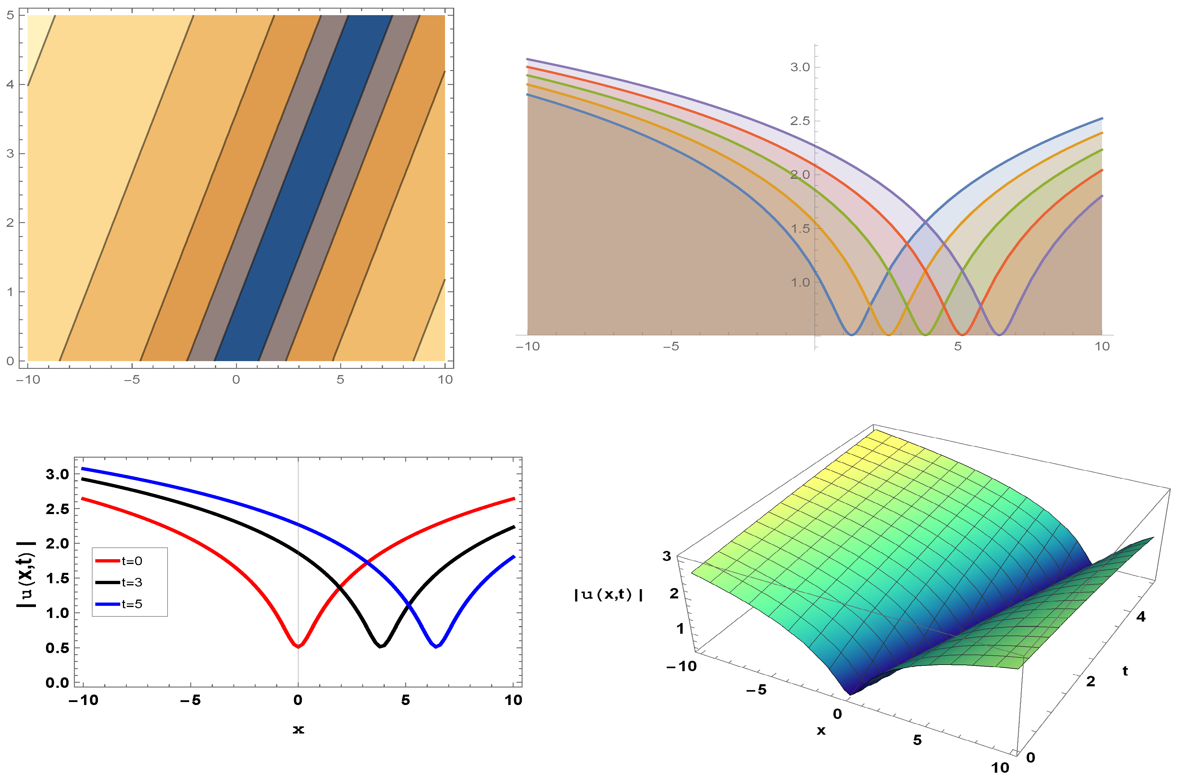
Abstract

In this article, a new version of the generalized q-deformed Sinh–Gordon equation is presented, and analytical solutions are developed for specific parameter sets using those equations. There is a possibility that the new equation can be used to model physical systems that have broken symmetries and include also effects related to amplification or dissipation. In addition, we have include some illustrations that depict the varied patterns of soliton propagation.

1. Introduction

Both in mathematics and applied sciences, dynamic models are essential. These models are built on differential equations, either ordinary or partial. A considerable impact on non-linearity is provided by the explanation of dynamics in microscopic systems that obey quantum physics principles [1,2,3]. Numerous scholars have explored a variety of ordinary or partial differential equations with significant applications in several fields [4,5,6,7,8,9,10].

The q-deformed non-linear equations have great interest in describing the behavior of some physical systems when they lose their symmetry, for example the deformed nucleus in nuclear reactions, phase change in solid state physics, the perturbation in the quantum optics, and elasticity changes [11,12,13,14,15]. Eleuch [16] introduced a new generalized form and new analytical solutions of the q-deformed equation.

$$\frac{{\partial }^{2}u}{\partial z\partial \zeta }={\left[sin{h}_q\left(u^{\gamma }\right)\right]}^p-\delta .$$

(1)

Equation (1) has been solved analytically and numerically using several methods in many papers [16,17,18,19,20]. In our paper [17], we introduced soliton solution of this equation using generalized projective Riccati equations (GPRE) and (-$\varphi (\xi$))-expansion methods. In another work, the ($G^{{}^{\prime }}/G$)-expansion approach and the exponential cubic B-spline algorithm are used to investigate the solutions of the same equation analytically and numerically [18]. The solutions 3+1 q-deformed equation is investigated by ($G^{{}^{\prime }}/G$)-expansion, finite element, and cubic b-spline techniques [19]. Moreover, the ($\frac{G^{{}^{\prime }}}{G},\frac{1}{G}$)-expansion and Sine–Gordon-expansion methods are applied to obtain new solutions of the (2+1)-dimensional q-deformed model, and the stability of the solutions was investigated using Painlevé analysis technique [20].

In this paper, as an extension of Equation (1) (Eleuch equation), we propose a new form of generalized q-deformed Sinh–Gordon equation as:

$$\frac{{\partial }^{2}u}{\partial z\partial \zeta }=e^{\alpha u}{\left[sin{h}_q\left(u^{\gamma }\right)\right]}^p-\delta .$$

(2)

where $\gamma ,p,\alpha \in {\mathbb{R}}^{*}$, $\delta \in \mathbb{R}$ and $0<q<1$.

The $sin{h}_q$ is defined by:

$$sin{h}_q\left(t\right)=\frac{e^t-q{e}^{-t}}{2}.$$

We explore the soliton solutions of (2) using a Kudryashov approach.

This paper is organized as follows: the second section introduces the analysis of the proposed equation. In the third section, the analytical approach is provided. The fourth section contains the solutions. We provide several figures for solutions in the fifth section. We conclude in the last section.

2. The Mathematical Examination of the Model

Using the standard transformation:

$$x=az+\frac{\zeta }{a},$$

$$t=az-\frac{\zeta }{a},$$

where a is an arbitrary constant, then (2) can be written as:

$$\frac{{\partial }^{2}u}{\partial x^2}-\frac{{\partial }^{2}u}{\partial t^2}=e^{\alpha u}{\left[sin{h}_q\left(u^{\gamma }\right)\right]}^p-\delta .$$

(3)

The transformation below is applied to find the traveling wave solution of (3).

$$u(x,t)=h\left(\xi \right),$$

(4)

where

$$\xi =\kappa x-\theta t.$$

(5)

where $\theta$ is the traveling wave speed. From (4) and (5) then (3) becomes,

$$\left({\kappa }^2-{\theta }^2\right)h^{″}\left(\xi \right)+\delta -e^{\alpha h\left(\xi \right)}{\left[{\sin \mathrm{h}}_q\left(h{\left(\xi \right)}^{\gamma }\right)\right]}^p=0.$$

(6)

Now we look at three cases for (6).

• Case one: $p=\gamma =\alpha =1, \delta =-\frac{q}{2}.$

Thus, (6) can be written as:

$$\left({\kappa }^2-{\theta }^2\right)h^{″}\left(\xi \right)-\frac{q}{2}-e^{h\left(\xi \right)}\left[{\sin \mathrm{h}}_q\left(h\left(\xi \right)\right)\right]=0.$$

(7)

We can multiply both sides of (7) by $h^{\prime }\left(\xi \right)$ and get the following equation after integration.

$$\frac{1}{2}\left(-\left({\theta }^2-{\kappa }^2\right)h^{\prime }{\left(\xi \right)}^2-\frac{1}{2}{e}^{2h\left(\xi \right)}\right)-C_1=0,$$

(8)

where $C_1$ is the integration constant.

Let

$$h\left(\xi \right)=\frac{1}{2}ln\left(v\left(\xi \right)\right).$$

(9)

Then, (8) becomes,

$$-8C_{1}v{\left(\xi \right)}^2+\left({\kappa }^2-{\theta }^2\right)v^{\prime }{\left(\xi \right)}^2-2v{\left(\xi \right)}^3=0.$$

(10)

Thus, we can solve (10), to find the solution of (3) in the first case.

• Case two:$\alpha =-1, \gamma =1, p=1, \delta =\frac{1}{2}.$

Equation (6) can be written as:

$$\left({\kappa }^2-{\theta }^2\right)h^{″}\left(\xi \right)+\frac{1}{2}-e^{-h\left(\xi \right)}\left[{\sin \mathrm{h}}_q\left(h\left(\xi \right)\right)\right]=0.$$

(11)

We can multiply both sides of (11) by $h^{\prime }\left(\xi \right)$ and get the following equation after integration.

$$\frac{1}{2}\left(\left({\kappa }^2-{\theta }^2\right)h^{\prime }{\left(\xi \right)}^2-\frac{1}{2}q{e}^{-2h\left(\xi \right)}\right)-C_3=0.$$

(12)

Let

$$h\left(\xi \right)=\frac{1}{2}ln\left(v\left(\xi \right)\right).$$

(13)

Then, (12) becomes,

$$\left({\kappa }^2-{\theta }^2\right)v^{\prime }{\left(\xi \right)}^2-2v\left(\xi \right)\left(4C_{3}v\left(\xi \right)+q\right)=0.$$

(14)

Then, we can solve (14) to get solution of Equation (3) in the second case.

• Case three: Assume that $\alpha =2, \gamma =1, p=2, \delta ={\left(\frac{q}{2}\right)}^2.$

Then, (6) can be written as:

$$\left({\kappa }^2-{\theta }^2\right)h^{″}\left(\xi \right)-e^{2h\left(\xi \right)}{\left[{\sin \mathrm{h}}_q\left(h\left(\xi \right)\right)\right]}^2+{\left(\frac{q}{2}\right)}^2=0.$$

(15)

By multiplying both sides of (15) by $h^{\prime }\left(\xi \right)$ we get after integration.

$$\frac{1}{4}\left(q{e}^{2h\left(\xi \right)}-2\left({\theta }^2-{\kappa }^2\right)h^{\prime }{\left(\xi \right)}^2-\frac{1}{4}{e}^{4h\left(\xi \right)}\right)-C_5=0.$$

(16)

Let

$$h\left(\xi \right)=ln\left(v\right(\xi \left)\right).$$

(17)

Then, (16) becomes,

$$-16C_{5}v{\left(\xi \right)}^2+4qv{\left(\xi \right)}^4+8\left({\kappa }^2-{\theta }^2\right)v^{\prime }{\left(\xi \right)}^2-v{\left(\xi \right)}^6=0.$$

(18)

We can solve (18) to find the solution of (3) in the third case.

3. The Strategy of the Kudryashov Technique

Let us consider the following form of the partial differential equation:

$$G(u,u_{xx},u_{tt},...)=0.$$

(19)

To convert (3) to an ordinary differential equation, we apply the traveling wave transformation:

$$H(h,h^{″},...)=0.$$

(20)

The following are the key steps in the new generalization of the Kudryashov method:

Step 1:

Suppose the solution of (20) can be expressed as follows:

$$h\left(\xi \right)=\sum _{i=0}^N(A_i{\left(Q\left(\xi \right)\right)}^i,$$

(21)

where $A_i(i=0,1,2,...,N), A_N\ne 0$ are constants that may be found using the homogeneous balancing principle that determines N.

Step 2:

The ordinary differential equation is fulfilled by the function $Q\left(\xi \right)$:

$$\frac{dQ\left(\xi \right)}{d\xi }=(Q\left(\xi \right)-1)Q\left(\xi \right).$$

(22)

The solution to (22) is as follows:

$$Q\left(\xi \right)=\frac{1}{1+e^{\xi }}.$$

(23)

Step 3:

We get a polynomial of $Q\left(\xi \right)$ by putting (21) into (20). We obtain a set of algebraic equations by combining all terms with similar powers of $Q\left(\xi \right)$ and setting each coefficient to zero.

Step 4:

We determine the solution of (19) by solving this system.

4. Soliton Solutions for the Model

The Kudryashov method is used in this section to obtain the analytic solution to the three cases specified for the problem (3).

• Case1:$\mathbf{\alpha }=\mathit{p}=\mathbf{\gamma }=\mathbf{1}\mathbf{,} \mathbf{\delta }=-\frac{\mathit{q}}{\mathbf{2}}$:

In (10) by considering first vanishing integration constant we get the following solution:

$$v\left(\xi \right)=\frac{4}{\left(C_2+\xi \sqrt{\frac{2}{{\kappa }^2-{\theta }^2}}\right){}^2}.$$

(24)

Then, by using (9) with (5) and (4) we get the following solution to (3)

$$u(x,t)=\frac{1}{2}ln\left(\frac{4}{\left(C_2+(\kappa x-\theta t)\sqrt{\frac{2}{{\kappa }^2-{\theta }^2}}\right){}^2}\right).$$

(25)

In (10), if constant of integration non-zero we apply the balance principle in (10) between $v^{\prime 2}$ and $v^3$ we get $2N+2=3N\Rightarrow N=2$. The solution of (10) can be written as follows:

$$v\left(\xi \right)=\sum _{i=0}^2{A}_i{(Q\left(\xi \right)}^i.$$

(26)

We obtain the system by substituting (26) into (10) and setting the coefficient of $Q\left(\xi \right)$ to zero:

$$-8A_0^2{C}_1-2A_0^3=0,$$

$$-16A_1{A}_0{C}_1-6A_1{A}_0^2=0,$$

$$-16A_2{A}_0{C}_1-8A_1^2{C}_1-A_1^2{\theta }^2+A_1^2{\kappa }^2-6A_2{A}_0^2-6A_1^2{A}_0=0,$$

$$-16A_2{A}_1{C}_1+2A_1^2{\theta }^2-4A_2{A}_1{\theta }^2-2A_1^2{\kappa }^2+4A_2{A}_1{\kappa }^2$$

$$-2A_1^3-12A_0{A}_2{A}_1=0,$$

$$-8A_2^2{C}_1-4A_2^2{\theta }^2+8A_1{A}_2{\theta }^2-A_1^2{\theta }^2+A_1^2{\kappa }^2$$

$$+4A_2^2{\kappa }^2-8A_1{A}_2{\kappa }^2-6A_0{A}_2^2-6A_1^2{A}_2=0,$$

$$8A_2^2{\theta }^2-4A_1{A}_2{\theta }^2-8A_2^2{\kappa }^2+4A_1{A}_2{\kappa }^2-6A_1{A}_2^2=0,$$

$$-4A_2^2{\theta }^2+4A_2^2{\kappa }^2-2A_2^3=0.$$

We can determine the constants by solving the above equations by symbolic software, such as Mathematica.

$$A_0=0,A_1=-16C_1,A_2=16C_1,\kappa =\mp \sqrt{8C_1+{\theta }^2}.$$

(27)

Then, the solutions for (3) at $\alpha =p=\gamma =1, \delta =-\frac{q}{2}$ by substituting (27) into (26) with (9), (5), and (4).

$$\begin{array}{cc}\hfill u_{1,2}(x,t)& =\frac{1}{2}ln\left(\frac{-16C_1}{1+e^{(\kappa x-\theta t)}}+\frac{16C_1}{{(1+e^{(\kappa x-\theta t)})}^2}\right).\hfill \end{array}$$

(28)

• Case 2:$\mathbf{\alpha }=-\mathbf{1}\mathbf{,} \mathbf{\gamma }=\mathbf{1}\mathbf{,} \mathit{p}=\mathbf{1}\mathbf{,} \mathbf{\delta }=\frac{\mathbf{1}}{\mathbf{2}}$:

In (14), if the constant of integration equal zero we have:

$$v\left(\xi \right)=\frac{1}{4}\left(C_4+\xi \sqrt{\frac{2q}{{\kappa }^2-{\theta }^2}}\right){}^2.$$

(29)

Then, by using (13) with (5) and (4) we get the following solution to (3)

$$u(x,t)=\frac{1}{2}ln\left(\frac{1}{4}\left(C_4+(\kappa x-\theta t)\sqrt{\frac{2q}{{\kappa }^2-{\theta }^2}}\right){}^2\right).$$

(30)

In (14), if constant of integration is not equal zero we apply the balance principle in (14) between $v^{\prime 2}$ and $v^2$ we get $2N+2=2N$ we cannot find N so, we take this transformation

$$v\left(\xi \right)=\frac{1}{f\left(\xi \right)}.$$

(31)

Then, (14) becomes

$$-8C_{3}f{\left(\xi \right)}^2+\left({\kappa }^2-{\theta }^2\right)f^{\prime }{\left(\xi \right)}^2-2qf{\left(\xi \right)}^3=0.$$

(32)

Now, we apply the balance principle in (32) between $f^{\prime 2}$ and $f^3$ we get $2N+2=3N\Rightarrow N=2$.

The solution of (32) can be written as follows:

$$f\left(\xi \right)=\sum _{i=0}^2{A}_i{(Q\left(\xi \right)}^i.$$

(33)

We obtain the system of equations by substituting (33) into (32) and setting the coefficient of $Q\left(\xi \right)$ to zero:

$$-8A_0^2{C}_3-2A_0^{3}q=0,$$

$$-16A_1{A}_0{C}_3-6A_1{A}_0^{2}q=0,$$

$$-16A_2{A}_0{C}_3-8A_1^2{C}_3-A_1^2{\theta }^2+A_1^2{\kappa }^2-6A_2{A}_0^{2}q-6A_1^2{A}_{0}q=0,$$

$$-16A_2{A}_1{C}_3+2A_1^2{\theta }^2-4A_2{A}_1{\theta }^2-2A_1^2{\kappa }^2$$

$$+4A_2{A}_1{\kappa }^2-2A_1^{3}q-12A_0{A}_2{A}_{1}q=0,$$

$$-8A_2^2{C}_3-4A_2^2{\theta }^2+8A_1{A}_2{\theta }^2-A_1^2{\theta }^2+A_1^2{\kappa }^2$$

$$+4A_2^2{\kappa }^2-8A_1{A}_2{\kappa }^2-6A_0{A}_2^{2}q-6A_1^2{A}_{2}q=0,$$

$$8A_2^2{\theta }^2-4A_1{A}_2{\theta }^2-8A_2^2{\kappa }^2+4A_1{A}_2{\kappa }^2-6A_1{A}_2^{2}q=0,$$

$$-4A_2^2{\theta }^2+4A_2^2{\kappa }^2-2A_2^{3}q=0.$$

We get the following constants by using the Mathematica program to solve the previous set of equations.

$$A_0=0,A_1=-\frac{16C_3}{q},A_2=\frac{16C_3}{q},\kappa =\mp \sqrt{8C_3+{\theta }^2}.$$

(34)

Then, the solutions of (3) for $\alpha =-1, \gamma =1, p=1, \delta =\frac{1}{2}$ by substituting (34) into (33) with (31), (13), (5), and (4).

$$\begin{array}{cc}\hfill u_{1,2}(x,t)& =\frac{1}{2}ln\left(\frac{1}{\frac{-\frac{16C_3}{q}}{1+e^{(\kappa x-\theta t)}}+\frac{\frac{16C_3}{q}}{{(1+e^{(\kappa x-\theta t)})}^2}}\right).\hfill \end{array}$$

(35)

• Case 3:$\mathbf{\alpha }=\mathbf{2}\mathbf{,} \mathbf{\gamma }=\mathbf{1}\mathbf{,} \mathit{p}=\mathbf{2}\mathbf{,} \mathbf{\delta }={\left(\frac{\mathit{q}}{\mathbf{2}}\right)}^{\mathbf{2}}$:

By applying the balance principle in (18) between $v^{\prime 2}$ and $v^6$ we get $2N+2=6N\Rightarrow N=\frac{1}{2}$ but N integer number. So, we consider this transformation

$$v\left(\xi \right)=f{\left(\xi \right)}^{\frac{1}{2}}.$$

(36)

Then, (18) becomes:

$$-16C_{5}f{\left(\xi \right)}^2-2\left({\theta }^2-{\kappa }^2\right)f^{\prime }{\left(\xi \right)}^2+4qf{\left(\xi \right)}^3-f{\left(\xi \right)}^4=0.$$

(37)

Now, we apply the balance principle in (37) between $f^{\prime 2}$ and $f^4$ we get $2N+2=4N\Rightarrow N=1$. So, the solution of (37) can be written as follows:

$$f\left(\xi \right)=\sum _{i=0}^1{A}_i{(Q\left(\xi \right)}^i.$$

(38)

We get the following system by substituting (38) into (37) and setting the coefficient of $Q\left(\xi \right)$ to zero:

$$-16A_0^2{C}_5+4A_0^{3}q-A_0^4=0,$$

$$-32A_1{A}_0{C}_5+12A_1{A}_0^{2}q-4A_1{A}_0^3=0,$$

$$-16A_1^2{C}_5-2A_1^2{\theta }^2+2A_1^2{\kappa }^2+12A_0{A}_1^{2}q-6A_0^2{A}_1^2=0,$$

$$4A_1^2{\theta }^2-4A_1^2{\kappa }^2+4A_1^{3}q-4A_0{A}_1^3=0,$$

$$-2A_1^2{\theta }^2+2A_1^2{\kappa }^2-A_1^4=0.$$

We get the following two sets of constants.

• Set one:

$$A_0=0,A_1=2q,\kappa =\mp \sqrt{{\theta }^2+2q^2},C_5=\frac{q^2}{4}.$$

(39)

Then, the solutions of (3) for $\alpha =2, \gamma =1, p=2, \delta ={\left(\frac{q}{2}\right)}^2$ by substituting (39) into (38) with (36), (17), (5), and (4).

$$\begin{array}{cc}\hfill u_{1,2}(x,t)& =\frac{1}{2}ln\left(\frac{2q}{1+e^{(\kappa x-\theta t)}}\right).\hfill \end{array}$$

(40)

• Set two:

$$A_0=2q,A_1=-2q,\kappa =\mp \sqrt{{\theta }^2+2q^2},C_5=\frac{q^2}{4}.$$

(41)

Then, the solutions of (3) for $\alpha =2, \gamma =1 ,p=2, \delta ={\left(\frac{q}{2}\right)}^2$ by substituting (41) into (38) with (36), (17), (5), and (4).

$$\begin{array}{cc}\hfill u_{3,4}(x,t)& =\frac{1}{2}ln\left(2q+\frac{-2q}{1+e^{(\kappa x-\theta t)}}\right).\hfill \end{array}$$

(42)

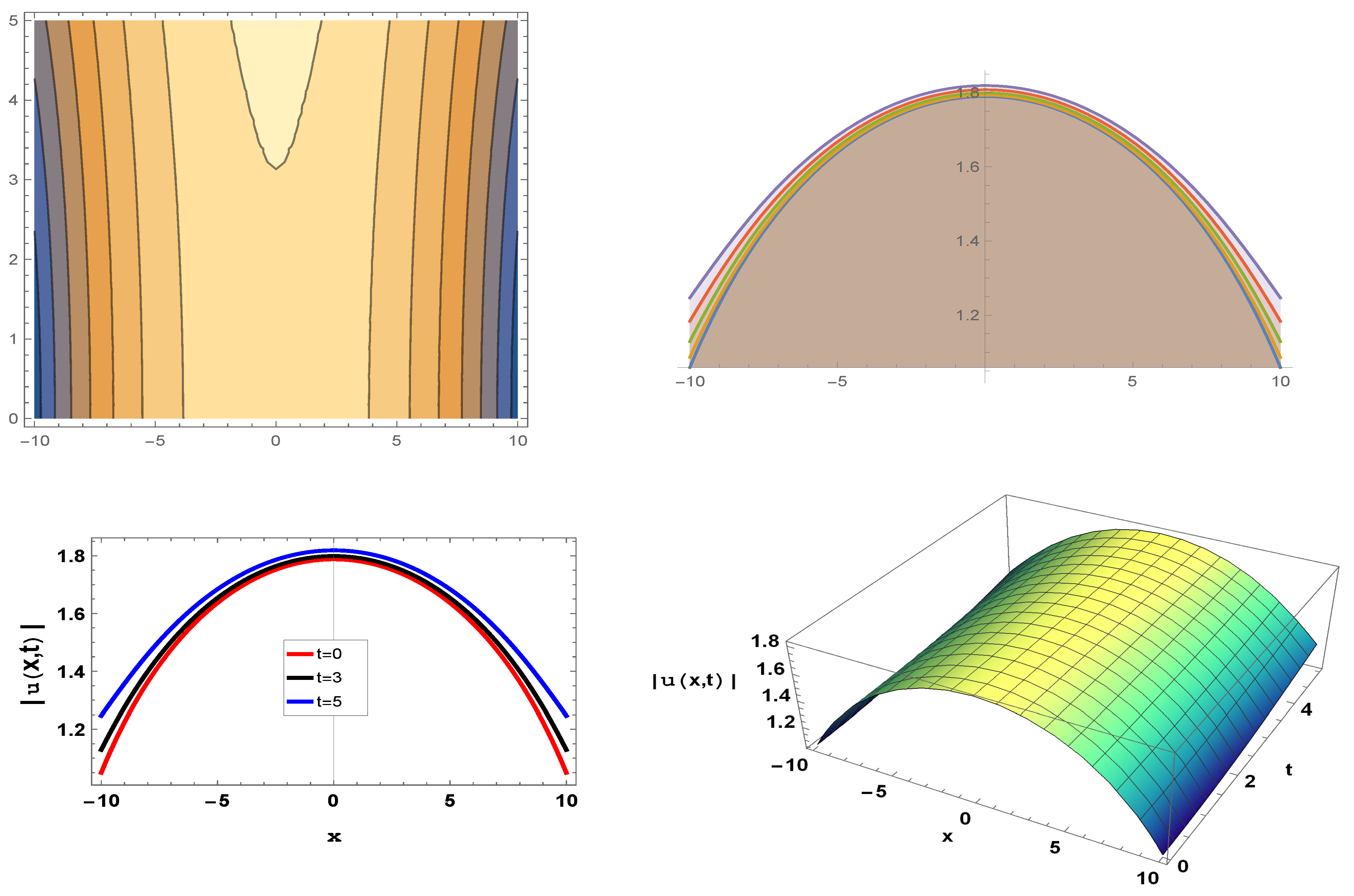
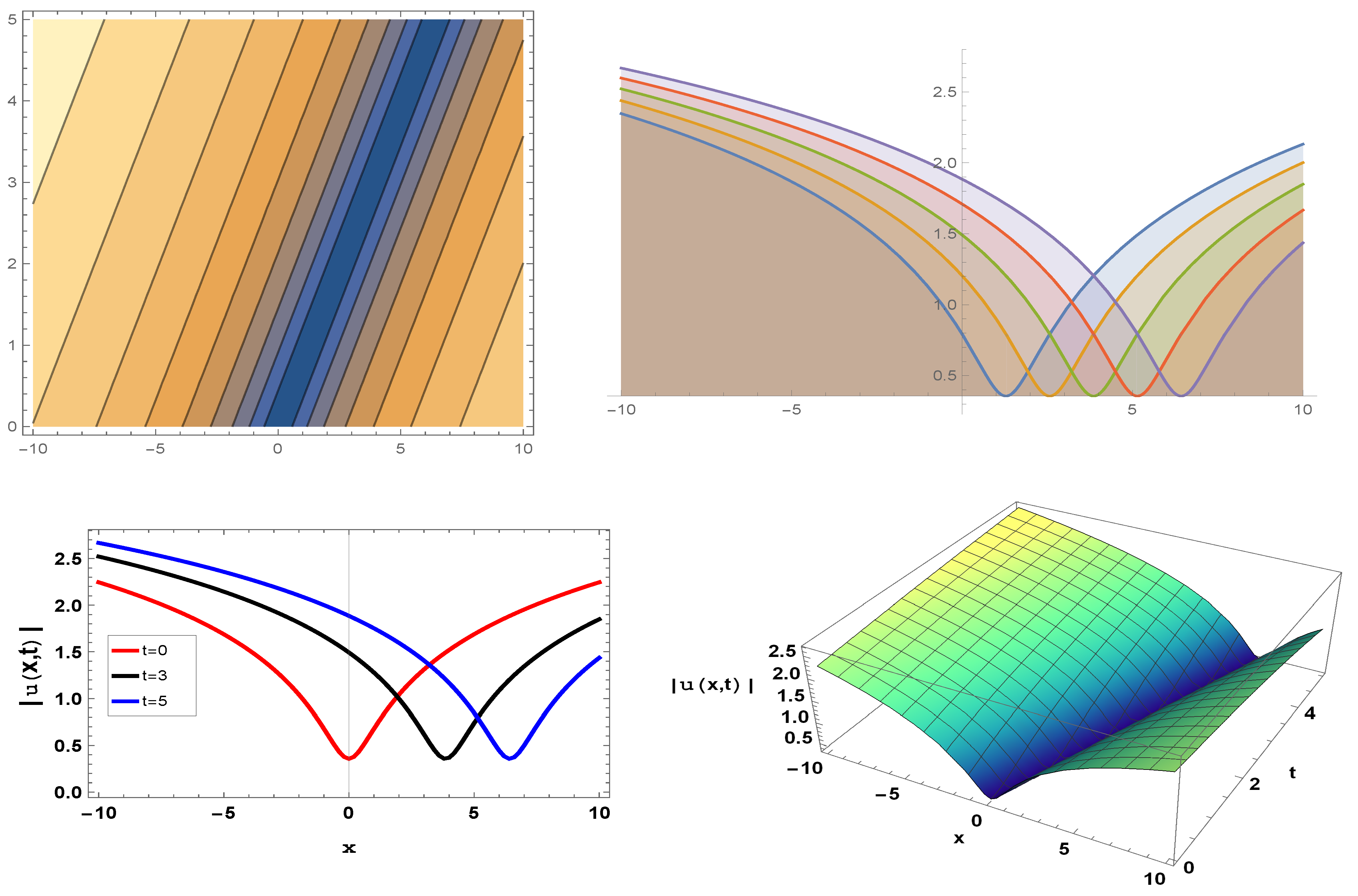
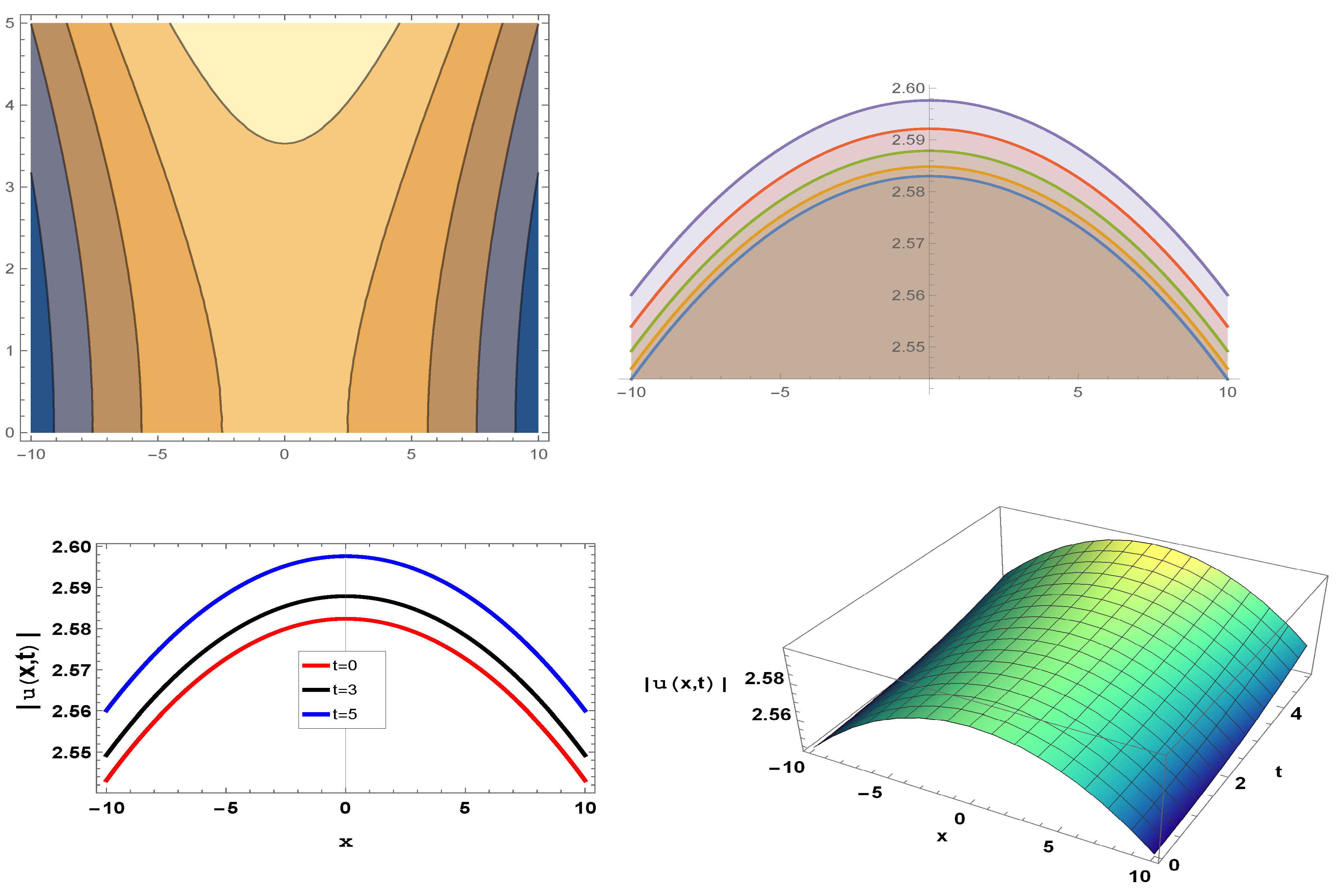
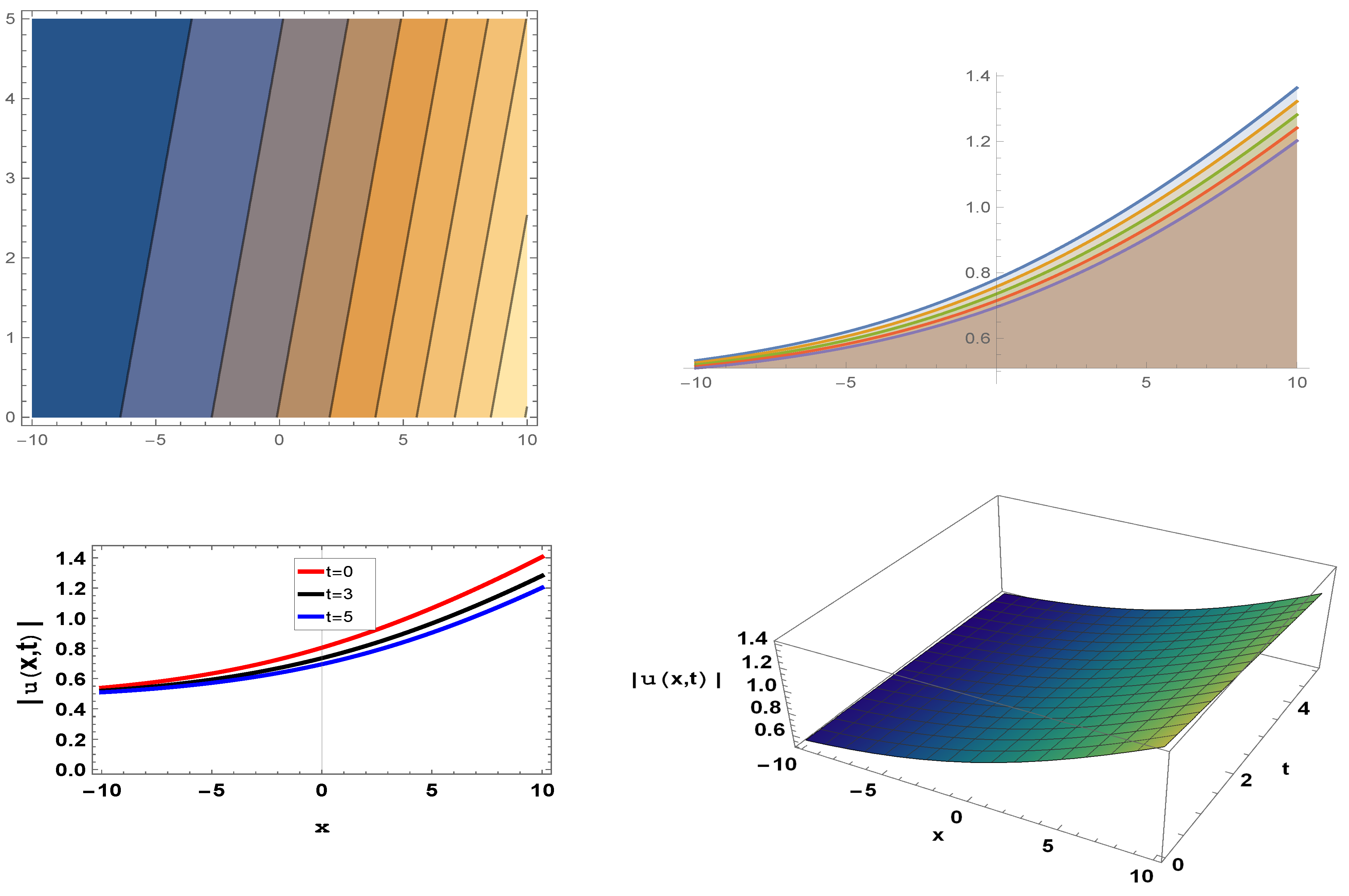
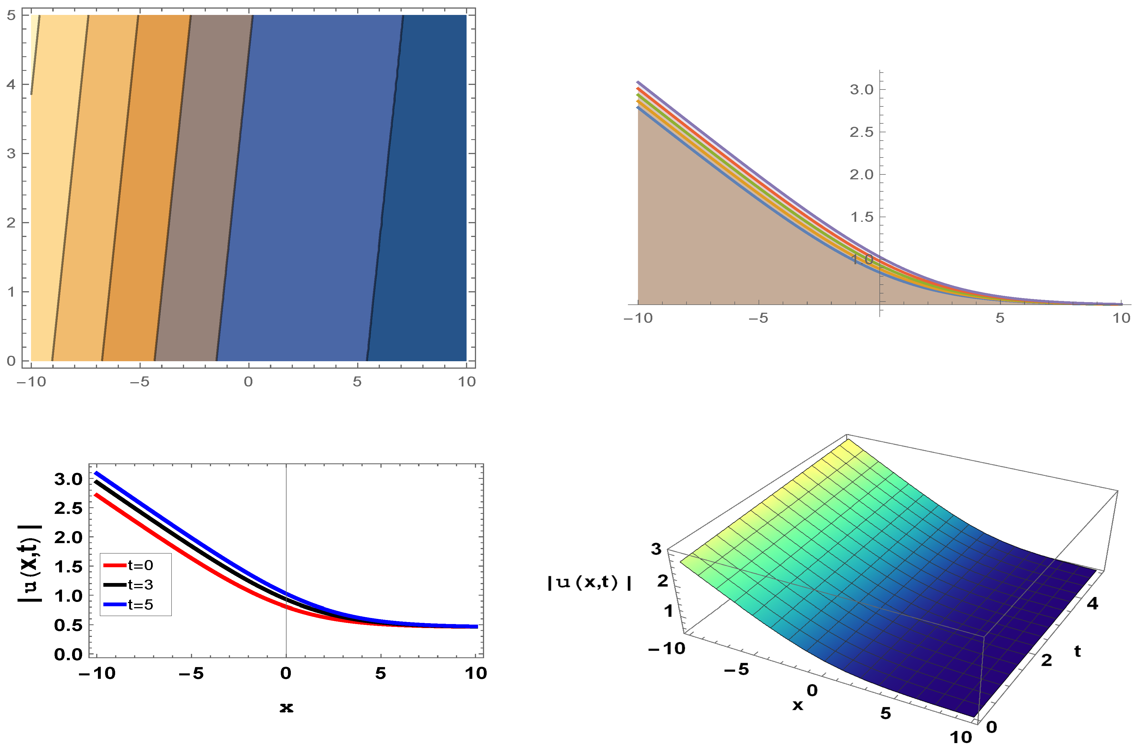
5. Illustrations with Graphics

Here, we illustrate some two-dimensional, three-dimensional, and contour figures of obtained solutions. Figure 1, Figure 2, Figure 3, Figure 4, Figure 5 and Figure 6 depicts some of the analytical solutions. Firstly, we introduce two figures of case 1 for $p=\gamma =\alpha =1, \delta =-\frac{q}{2}$. In Figure 1, we present the graph of (25) for $C_2=1.2, \theta =0.09, \kappa =0.07$ we observe that the wave moves to the right when the time increases. In addition, Figure 2 shows the graph of (28) $q=0.5$, $\theta =0.1, C_1=-0.007$ we notice that the wave goes up over time. Secondly, we present two figures of case 1 for $\alpha =-1, \gamma =1, p=1, \delta =\frac{1}{2}$. Figure 3 shows the graph of (30) for $C_4=1.4, \theta =0.09, \kappa =0.07, q=0.4$ we observe that the wave is moving to the right over time. The graph of (34) at $C_3=-0.001, \theta =0.07, q=0.7$ is presented in Figure 4, we notice that the wave moves up over time. Thirdly, we plot two figures of case 1 for $\alpha =2, \gamma =1, p=2, \delta ={\left(\frac{q}{2}\right)}^2$. The graph of (39) at $\theta =0.25, q=0.2$ is illustrated in Figure 5, we note that the wave moves down over time. Finally, in Figure 6, we show the graph of (42) at $\theta =0.25, q=0.2$ we notice that the wave amplitude grows when the time evolves.

6. Conclusions

A new generalized form of the q-deformed Sinh–Gordon equation is developed and investigated in this study. The Kudryashov approach is utilized in order to locate the analytical soliton solutions. The method used is effective and gives good results that can be easily interpreted. The consideration of three different examples relating to the proposed equation is expanded upon. We have provided an illustration of the adequacy of the wave propagation. In the future works, we will expect to develop alternative methods for solving this form of q-deformed Sinh–Gordon equation. The newly presented equation makes it possible to describe physical systems that break symmetry where in addition amplification or dissipation effects could be considered.

References

- Yusuf, A.; Sulaiman, T.A.; Mirzazadeh, M.; Hosseini, K. M-truncated optical solitons to a nonlinear Schrodinger equation describing the pulse propagation through a two-mode optical fiber. Opt. Quantum. Electron. 2021, 53, 1–17. [Google Scholar] [CrossRef]
- Boutabba, N. Kerr-effect analysis in a three-level negative index material under magneto cross-coupling. J. Opt. 2018, 20, 025102. [Google Scholar] [CrossRef]
- Kilbas, A.A.; Srivastava, H.M.; Trujillo, J.J. Theory and Applications of Fractional Differential Equations; Elsevier: Amsterdam, The Netherlands, 2006. [Google Scholar]
- Lanre, A.; Mohammad, M.; Kamyar, H. Solitons and other solutions of perturbed nonlinearBiswas–Milovic equation with Kudryashov’s lawof refractive index. Nonlinear Anal. Model. Control. 2022, 27, 479–495. [Google Scholar]
- Abdel-Aty, A.H.; Khater, M.M.; Attia, R.A.; Abdel-Aty, M.; Eleuch, H. On the New Explicit Solutions of the Fractional Nonlinear Spacetime Nuclear Model. Fractals 2020, 28, 2040035. [Google Scholar] [CrossRef]
- Raslan, K.R.; Ali, K.K. Numerical study of MHD-duct flow using the two-dimensional finite difference method. Appl. Math. Inf. Sci. 2020, 14, 693–697. [Google Scholar]
- Boutabba, N.; Eleuch, H.; Bouchriha, H. Thermal bath effect on soliton propagation in three-level atomic system. Synth. Met. 2009, 159, 1239–1243. [Google Scholar] [CrossRef]
- Zafar, A.; Raheel, M.; Ali, K.K.; Razzaq, W. On optical soliton solutions of new Hamiltonian amplitude equation via Jacobi elliptic functions. Eur. Phys. J. Plus 2020, 135, 674. [Google Scholar] [CrossRef]
- Eleuch, H.; Nessib, N.B.; Bennaceur, R. Quantum Model of emission in weakly non ideal plasma. Eur. Phys. J. D 2004, 29, 391. [Google Scholar] [CrossRef]
- Saha, A.; Ali, K.K.; Rezazadeh, H.; Ghatani, Y. Analytical optical pulses and bifurcation analysis for the traveling optical pulses of the hyperbolic nonlinear Schrödinger equation. Opt. Quantum Electron. 2021, 53, 150. [Google Scholar] [CrossRef]
- Sharifi, B.; Naderi, D. The effect of deformation and orientation of colliding nuclei on synthesis of superheavy elements. Nucl. Phys. A 2019, 991, 121616. [Google Scholar] [CrossRef]
- Lynch, D.R.; O’Neill, K. Continuously deforming finite elements for the solution of parabolic problems, with and without phase change. Int. J. Numer. Meth. Engng. 1981, 17, 81–96. [Google Scholar] [CrossRef]
- Ching, C.L.; Ng, W.K. Generalized coherent states under deformed quantum mechanics with maximum momentum. Phys. Rev. D 2013, 88, 084009. [Google Scholar] [CrossRef]
- Berra-Montiel, J.; Molgado, A. Coherent representation of fields and deformation quantization. Int. J. Geom. Methods Mod. Phys. 2020, 17, 2050166. [Google Scholar] [CrossRef]
- Holmes, D.P. Elasticity and stability of shape-shifting structures. Curr. Opin. Colloid Interface Sci. 2019, 40, 118–137. [Google Scholar] [CrossRef]
- Eleuch, H. Some analytical solitary wave solutions for the generalized q-deformed Sinh-Gordon equation Hindawi Adv. Math. Phys. 2018, 2018, 5242757. [Google Scholar]
- Raza, N.; Arshed, S.; Alrebdi, H.I.; Abdel-Aty, A.H.; Eleuch, H. Abundant new optical soliton solutions related to q-deformed Sinh-Gordon model using two innovative integration architectures. Results Phys. 2022, 35, 105358. [Google Scholar] [CrossRef]
- Ali, K.K.; Abdel-Aty, A.H.; Eleuch, H. New soliton solutions for the conformal time derivative q-deformed physical model. Results Phys. 2022, 42, 105993. [Google Scholar] [CrossRef]
- Ali, K.K.; Al-Harbi, N.; Abdel-Aty, A.H. Traveling wave solutions to (3 + 1) conformal time derivative generalized q-deformed Sinh-Gordon equation. Alex. Eng. J. 2023, 65, 233–243. [Google Scholar] [CrossRef]
- Alrebdi, H.I.; Raza, N.; Arshed, S.; Butt, A.R.; Abdel-Aty, A.H.; Cesarano, C.; Eleuch, H. A Variety of New Explicit Analytical Soliton Solutions of q-Deformed Sinh-Gordon in (2+1) Dimensions. Symmetry 2022, 14, 2425. [Google Scholar] [CrossRef]
Disclaimer/Publisher’s Note: The statements, opinions and data contained in all publications are solely those of the individual author(s) and contributor(s) and not of MDPI and/or the editor(s). MDPI and/or the editor(s) disclaim responsibility for any injury to people or property resulting from any ideas, methods, instructions or products referred to in the content. |
© 2023 by the authors. Licensee MDPI, Basel, Switzerland. This article is an open access article distributed under the terms and conditions of the Creative Commons Attribution (CC BY) license (https://creativecommons.org/licenses/by/4.0/).
Share and Cite
Ali, K.K.; Alrebdi, H.I.; Alsaif, N.A.M.; Abdel-Aty, A.-H.; Eleuch, H.