Article

Vacuum Polarization of a Quantized Scalar Field in the Thermal State on the Short Throat Wormhole Background

N. I. Lobachevsky Institute of Mathematics and Mechanics, Kazan Federal University, Kremlevskaya Street 18, 420008 Kazan, Russia
*
Author to whom correspondence should be addressed.
Symmetry 2023, 15(2), 426; https://doi.org/10.3390/sym15020426
Submission received: 8 December 2022 / Revised: 8 January 2023 / Accepted: 3 February 2023 / Published: 6 February 2023

Abstract

:
Vacuum polarization of a scalar field on the short throat wormhole background is investigated. The scalar field is assumed to be massless, having an arbitrary coupling to the scalar curvature of spacetime. In addition, it is supposed that the field is in a thermal state with an arbitrary temperature.

1. Introduction

Two important quantities in the study of quantum effects in strong gravitational fields are ϕ 2 and T μ ν where ϕ is a quantized field and T μ ν is the stress tensor for this field. These quantities provide us with information about spontaneous symmetry breaking, particle production, and vacuum–polarization effects. In addition, T μ ν is the source of the backreaction effect of the quantized fields on the geometry of spacetime. This effect is described using the semi-classical theory of gravity
G ν μ = 8 π T ν μ .
It should be noted that vacuum fluctuations of quantum fields were considered as matter, providing the existence of wormholes in [1,2,3,4].
The main problem of the semi-classical theory of gravity is that the contribution of the quantized gravitational field is not taken into account. A popular solution to this problem is the limit of a large number of matter fields. In this limit, it is assumed that the number of matter fields present is so large that the graviton contribution is negligible. Another problem of this theory is that the effects of vacuum polarization are generally determined by the topological and geometric properties of spacetime as a whole and the choice of the quantum state in which the vacuum expectation values are calculated. This means that calculating the functional dependence T ν μ on the metric tensor, which must be determined from Equation (1), is extremely difficult. Such calculations T μ ν and ϕ 2 have been made only in a highly symmetrical spacetime for conformally invariant fields and Equation (1) has been solved by [5,6,7,8,9].
Usually, numerical calculations ϕ 2 and T ν μ are extremely difficult [10,11,12,13,14,15,16,17]. In some cases, ϕ 2 and T μ ν are determined by the local properties of spacetime. In these cases, it is possible to approximate the functional dependence of ϕ 2 and T μ ν on the metric tensor. One of the most well-known examples of such a situation is the case of a very massive field. In this case, the field mass m is much greater than 1 / l , where l is the characteristic curvature scale of the background geometry
1 m l 1 ,
and ϕ 2 can be expanded in terms of the powers of m l [18,19,20,21,22,23,24].
We emphasize that the only parameter of the length dimension in the problem (1) is the Planck length of the l P l . This means that the characteristic scale l of the curvature of the spacetime can differ from l P l only if there is a large dimensionless parameter. As an example of such a parameter, we can consider the number of fields whose polarization is a source of spacetime curvature (Here and below, it is assumed, of course, that the characteristic scale of change of the background gravitational field is sufficiently greater than l P l , so that the very notion of a classical spacetime still has some meaning.). In the case of a massive field, the existence of an additional parameter, 1 / m l , does not increase the characteristic curvature scale l, which corresponds to the solution of Equation (1) (The characteristic scale of components G ν μ on the left-hand side of Equation (1) is 1 / l 2 and, on the right-hand side, is l P l 2 / ( m 2 l 6 ) ). For massless quantized fields, this parameter can be the field coupling constants with spacetime curvature [4]. Another possibility of introducing an additional parameter into the problem (1) is to consider the non-zero temperature of the quantum state for a quantum field. It is known (see, e.g., [25]) that, in the high temperature limit (when T 1 / l , T is the thermal state temperature), ϕ 2 , for such a thermal state, is proportional to T 2 .
In this work, we investigate the quantized scalar field in the wormhole spacetime with an infinitely short throat. It is assumed that the field is massless, has an arbitrary coupling to the scalar curvature of spacetime, and is in the thermal state with the arbitrary temperature. We calculate φ 2 using the point-splitting method and demonstrate that the result has correct asymptotics at high temperature and at T = 0 .
The units = c = G = k B = 1 are used throughout the paper.

2. Non-Renormalized Expression φ 2

The metric of a static spherically symmetric wormhole spacetime with an infinitely short throat, analytically extended into Euclidean space, has the form
d s 2 = d τ 2 + d ρ 2 + ( | ρ | + a ) 2 ( d θ 2 + sin 2 θ d φ 2 ) ,
where τ is the Euclidean time ( τ = i t and t is the coordinate corresponding to the time-like Killing vector, which always exists in static spacetime).
The vacuum expectation value of an operator ϕ 2 quantized scalar field ϕ can be calculated using the method of point splitting [26,27] from the Euclidean Green’s function G E ( x ; x ˜ ) as follows
ϕ 2 ( x , x ˜ ) u n r e n = G E ( x , x ˜ ) ,
where G E ( x , x ˜ ) obeys the equation
x ξ R ( x ) G E ( x , x ˜ ) = δ 4 ( x , x ˜ ) | g ( x ) | ,
x = g μ ν ( x ) μ ν is calculated for the metric (3), ξ is a scalar field coupling to the curvature R. In spacetime (3), one finds that δ 4 ( x , x ˜ ) / g ( x ) can be written as δ ( τ τ ˜ ) δ ( r , r ˜ ) δ ( Ω , Ω ˜ ) / r 2 ( d Ω 2 = d θ 2 + sin 2 θ d φ 2 ) . The delta function δ ( Ω , Ω ˜ ) can be expanded in terms of Legendre polynomials P l with the result that
δ ( Ω , Ω ˜ ) = l , m Y l m ( Ω ) Y l m * ( Ω ˜ ) = 1 4 π l = 0 ( 2 l + 1 ) P l ( cos γ ) ,
where cos γ cos θ cos θ ˜ + sin θ sin θ ˜ cos ( ϕ ϕ ˜ ) .
In this paper, it is assumed that the field is in a thermal state at temperature T, determined with respect to a time-like Killing vector. In this case, the Green’s function is periodic by τ τ ˜ with a period 1 T . In this case, δ ( τ τ ˜ ) has the form
δ ( τ τ ˜ ) = T n = e i n 2 π T ( τ τ ˜ ) .
then
G E ( x ; x ˜ ) = T 4 π n = e i n 2 π T ( τ τ ˜ ) l = 0 ( 2 l + 1 ) P l ( cos γ ) g n l ( ρ , ρ ˜ ) = T 4 π l = 0 ( 2 l + 1 ) P l ( cos γ ) g 0 l ( ρ , ρ ˜ ) + T 2 π n = 1 cos [ 2 π n T ( τ τ ˜ ) ] l = 0 ( 2 l + 1 ) P l ( cos γ ) g n l ( ρ , ρ ˜ ) ,
where g n l ( ρ , ρ ˜ ) satisfies the equation
d 2 d ρ 2 + 2 ( | ρ | + a ) d ( | ρ | + a ) d ρ d d ρ ( 2 π n T ) 2 + l ( l + 1 ) ( | ρ | + a ) 2 + ξ R g n l ( ρ , ρ ˜ ) = δ ( ρ , ρ ˜ ) ( | ρ | + a ) 2 .

2.1. n 0 Contribution

The g n l ( ρ , ρ ˜ ) for ρ > ρ ˜ , n 0 is provided by the expression (compare with article [28])
g n l ( ρ , ρ ˜ ) = K ν k ( a + ρ ) I ν k ( a + ρ ˜ ) ( a + ρ ) ( a + ρ ˜ ) ( 8 ξ 1 ) I ν ( x ) K ν ( x ) + x I ν ( x ) K ν ( x ) + I ν ( x ) K ν ( x ) ( 8 ξ 1 ) K ν 2 ( x ) + 2 x K ν ( x ) K ν ( x ) × K ν k ( a + ρ ) K ν k ( a + ρ ˜ ) ( a + ρ ) ( a + ρ ˜ ) ,
where k = 2 π n T , x = ρ / a .
Let us represent g n l ( ρ , ρ ˜ ) ( n 0 ) as follows
g n l ( ρ , ρ ˜ ) = g n l M ( ρ , ρ ˜ ) + g n l I ( ρ , ρ ˜ ) ,
where
g n l M ( ρ , ρ ˜ ) = K ν k ( a + ρ ) I ν k ( a + ρ ˜ ) ( a + ρ ) ( a + ρ ˜ ) , g n l I ( ρ , ρ ˜ ) = ( 8 ξ 1 ) I ν ( x ) K ν ( x ) + x I ν ( x ) K ν ( x ) + I ν ( x ) K ν ( x ) ( 8 ξ 1 ) K ν 2 ( x ) + 2 x K ν ( x ) K ν ( x ) × K ν k ( a + ρ ) K ν k ( a + ρ ˜ ) ( a + ρ ) ( a + ρ ˜ ) .

2.2. n = 0 Contribution

The solution of Equation (9) for n = 0 , ρ > ρ ˜ has the form
g 0 l ( ρ , ρ ˜ ) = g 0 l M ( ρ , ρ ˜ ) + g 0 l I ( ρ , ρ ˜ ) ,
where
g 0 l M ( ρ , ρ ˜ ) = ( ρ + a ) ( l + 1 ) ( ρ ˜ + a ) l 2 l + 1 , g 0 l I ( ρ , ρ ˜ ) = a 2 l + 1 ( 1 8 ξ ) ( ρ + a ) l 1 ( ρ ˜ + a ) l 1 2 ( 2 l + 1 ) ( l 4 ξ + 1 ) .

2.3. General Expression
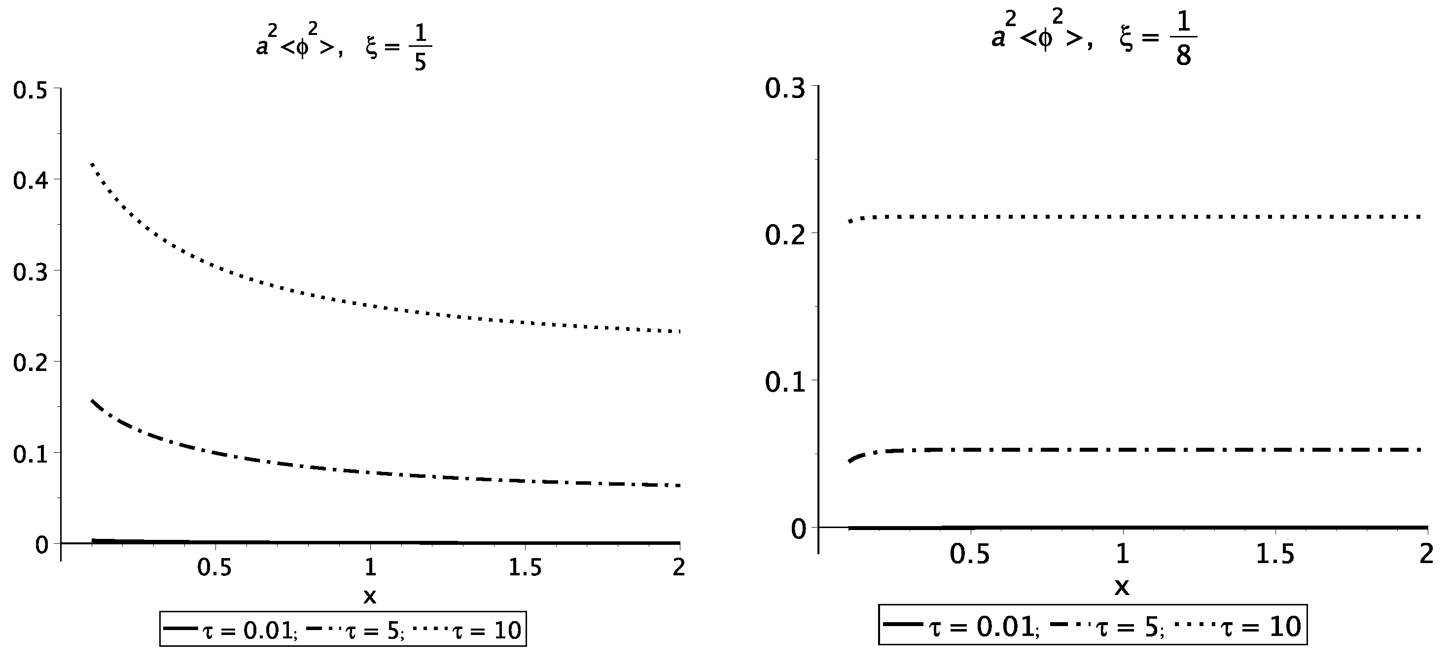
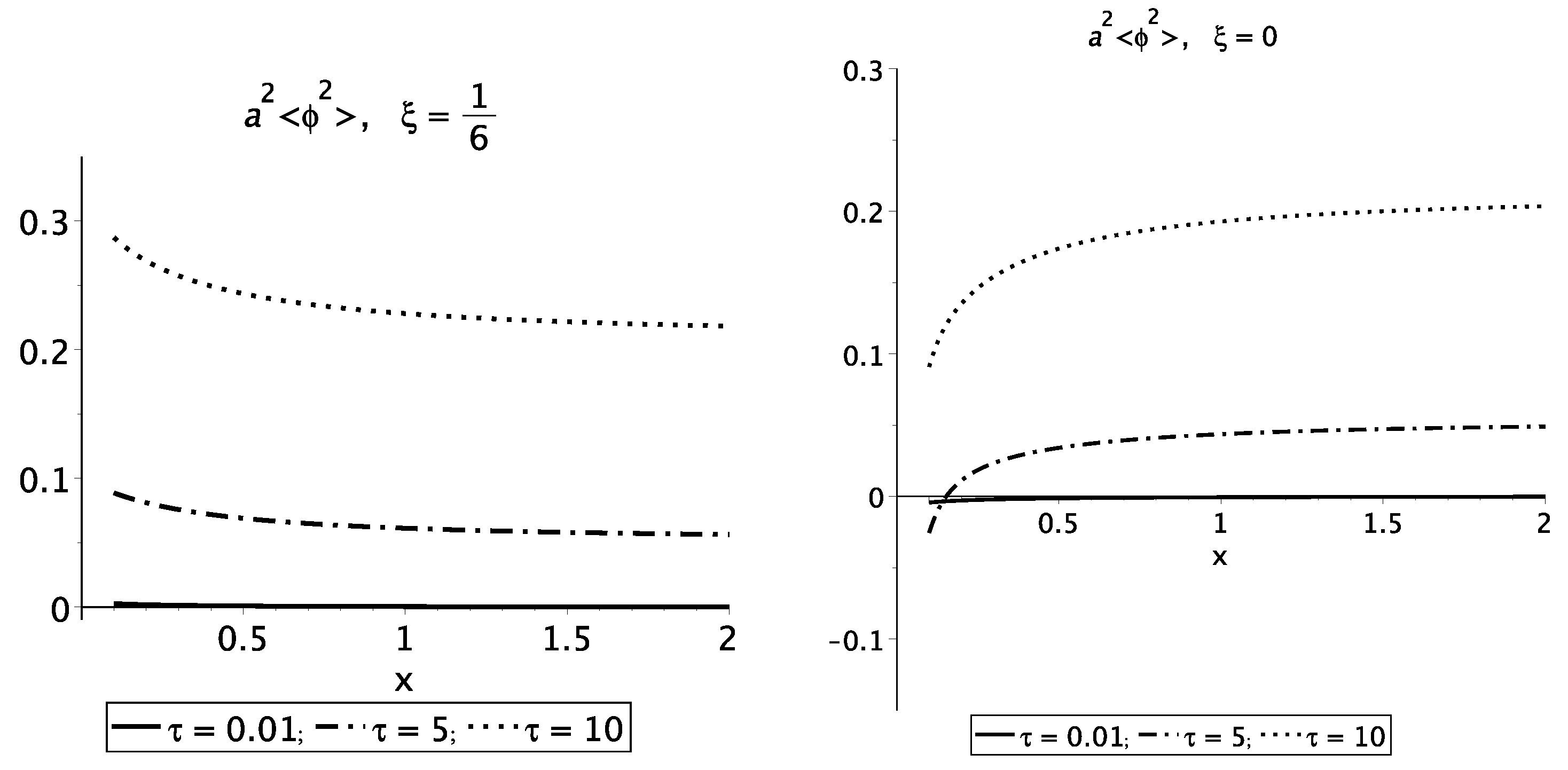
Hereafter, we will consider θ = θ ˜ , φ = φ ˜ . In this case, cos ( γ ) = 1 and P l ( 1 ) = 1 . Then, (8) will adopt the form
G E ( x ; x ˜ ) = T 4 π l = 0 ( 2 l + 1 ) g 0 l ( ρ , ρ ˜ ) + T 2 π n = 1 cos [ 2 π n T ( τ τ ˜ ) ] l = 0 ( 2 l + 1 ) g n l ( ρ , ρ ˜ ) .
Let us represent G E ( x ; x ˜ ) as
G E ( x ; x ˜ ) = G E 0 ( x ; x ˜ ) + G E n ( x ; x ˜ ) ,
where G E 0 ( x ; x ˜ ) is the first term in (13), and G E n ( x ; x ˜ ) is the last term in (13). Let us also represent each of these terms as
G E 0 ( x ; x ˜ ) = G E 0 M ( x ; x ˜ ) + G E 0 I ( x ; x ˜ ) , n = 0 , G E n ( x ; x ˜ ) = G E n M ( x ; x ˜ ) + G E n I ( x ; x ˜ ) , n 0 ,
and definitions of G E 0 M ( x ; x ˜ ) , G E 0 I ( x ; x ˜ ) , G E n M ( x ; x ˜ ) and G E n I ( x ; x ˜ ) are provided below. Let us define
G E n M ( τ , ρ ; τ ˜ , ρ ˜ ) T 2 π n = 1 cos 2 π n T ( τ τ ˜ ) l = 0 ( 2 l + 1 ) g n l M ( ρ , ρ ˜ ) .
Using the summation theorem for Bessel functions [29] and having performed the summation by n in (16), we will obtain
G E n M ( ρ ; ρ ˜ ) = 1 4 π 2 ( ρ ρ ˜ ) 2 T 4 π ( ρ ρ ˜ ) + T 2 12 T 4 π 2 ( ρ ρ ˜ ) 2 180 + O ( ( ρ ρ ˜ ) 3 )
for τ τ ˜ = 0 . Then, the definition G E n I ( τ , ρ ; τ ˜ , ρ ˜ ) has the form
G E n I ( τ , ρ ; τ ˜ , ρ ˜ ) = T 2 π n ˜ = 1 cos 2 π n T ( τ τ ˜ ) l = 0 ( 2 l + 1 ) g n l I ( ρ , ρ ˜ ) = T 2 π n = 1 cos 2 π n T ( τ τ ˜ ) l = 0 ( 2 l + 1 ) K ν k ( a + ρ ) K ν k ( a + ρ ˜ ) ( a + ρ ) ( a + ρ ˜ ) × ( 8 ξ 1 ) I ν ( k a ) K ν ( k a ) + k a I ν ( k a ) K ν ( k a ) + I ν ( k a ) K ν ( k a ) ( 8 ξ 1 ) K ν 2 ( k a ) + 2 k a K ν ( k a ) K ν ( k a )
Consequently,
G E n ( τ , ρ ; τ ˜ , ρ ˜ ) = G E n M ( ρ ; ρ ˜ ) + G E n I ( τ , ρ ; τ ˜ , ρ ˜ ) = 1 4 π 2 ( ρ ρ ˜ ) 2 T 4 π ( ρ ρ ˜ ) + T 2 12 T 4 π 2 ( ρ ρ ˜ ) 2 180 T 2 π n = 1 cos 2 π n T ( τ τ ˜ ) l = 0 ( 2 l + 1 ) K ν k ( a + ρ ) K ν k ( a + ρ ˜ ) ( a + ρ ) ( a + ρ ˜ ) × ( 8 ξ 1 ) I ν ( k a ) K ν ( k a ) + k a I ν ( k a ) K ν ( k a ) + I ν ( k a ) K ν ( k a ) ( 8 ξ 1 ) K ν 2 ( k a ) + 2 k a K ν ( k a ) K ν ( k a ) + O ( ( ρ ρ ˜ ) 3 ) .
We can denote (see (12))
G E 0 M ( ρ , ρ ˜ ) T 4 π l = 0 ( 2 l + 1 ) g 0 l M ( ρ , ρ ˜ ) = T 4 π l = 0 ( ρ + a ) ( l + 1 ) ( ρ ˜ + a ) l = T 4 π ( ρ ρ ˜ ) ,
G E 0 I ( ρ , ρ ˜ ) T 4 π l = 0 ( 2 l + 1 ) g 0 l I ( ρ , ρ ˜ ) = T 8 π l = 0 a 2 l + 1 ( 1 8 ξ ) ( ρ + a ) l 1 ( ρ ˜ + a ) l 1 ( l 4 ξ + 1 ) .
then
G E M ( ρ , ρ ˜ ) = G E 0 M ( ρ , ρ ˜ ) + G E n M ( ρ , ρ ˜ ) = 1 4 π 2 ( ρ ρ ˜ ) 2 + T 2 12 T 4 π 2 ( ρ ρ ˜ ) 2 180 + O ( ( ρ ρ ˜ ) 3 ) ,
G E I ( τ , ρ , τ ˜ , ρ ˜ ) = G E 0 I ( ρ , ρ ˜ ) + G E n I ( τ , ρ , τ ˜ , ρ ˜ ) = T 8 π l = 0 a 2 l + 1 ( 1 8 ξ ) ( ρ + a ) l 1 ( ρ ˜ + a ) l 1 ( l 4 ξ + 1 ) T 2 π n = 1 cos 2 π n T ( τ τ ˜ ) l = 0 ( 2 l + 1 ) K ν k ( a + ρ ) K ν k ( a + ρ ˜ ) ( a + ρ ) ( a + ρ ˜ ) × ( 8 ξ 1 ) I ν ( k a ) K ν ( k a ) + k a I ν ( k a ) K ν ( k a ) + I ν ( k a ) K ν ( k a ) ( 8 ξ 1 ) K ν 2 ( k a ) + 2 k a K ν ( k a ) K ν ( k a ) .
Finally,
G E ( τ , ρ , τ ˜ , ρ ˜ ) = G E I ( τ , ρ , τ ˜ , ρ ˜ ) + G E M ( ρ , ρ ˜ ) .
Then, the expression (8) can be rewritten as
G E ( τ , ρ ; τ , ρ ˜ ) = 1 4 π 2 ( ρ ρ ˜ ) 2 + T 2 12 T 4 π 2 ( ρ ρ ˜ ) 2 180 T 8 π l = 0 a 2 l + 1 ( 1 8 ξ ) ( ρ + a ) l 1 ( ρ ˜ + a ) l 1 ( l 4 ξ + 1 ) T 2 π n = 1 cos 2 π n T ( τ τ ˜ ) l = 0 ( 2 l + 1 ) × ( 8 ξ 1 ) I ν ( k a ) K ν ( k a ) + k a I ν ( k a ) K ν ( k a ) + I ν ( k a ) K ν ( k a ) ( 8 ξ 1 ) K ν 2 ( k a ) + 2 k a K ν ( k a ) K ν ( k a ) × K ν k ( a + ρ ) K ν k ( a + ρ ˜ ) ( a + ρ ) ( a + ρ ˜ ) + O ( ( ρ ρ ˜ ) 3 ) .
We can notice that G E M ( ρ , ρ ˜ ) coincides with the corresponding Green function of Minkowski spacetime.

3. Renormalization ϕ 2 and the Result

In this article, the point-splitting method is used for the regularization of ϕ 2 ( x , x ˜ ) . The renormalization procedure consists of subtracting G D S from G E ( x i , x ˜ i ) counterterm [27], which is equal to
G D S = 1 4 π 2 ( ρ ρ ˜ ) 2
in space (3) for x i x ˜ i = δ ρ i ( ρ ρ ˜ ) , and then letting ρ ˜ ρ . All the divergences of G E coincide with the divergences of G E M . Therefore, we will introduce
G E _ r e n M = lim ρ ˜ ρ G E M G D S .
Then, in the domain ρ > 0
a 2 ϕ 2 r e n = a 2 ( G E G D S ) = a 2 lim ρ ˜ ρ G E _ r e n M + G E I = a 2 T 2 12 + a 2 lim ρ ˜ ρ G E I = τ 2 48 π 2 τ 16 π 2 l = 0 ( 1 8 ξ ) ( l 4 ξ + 1 ) ( x + 1 ) 2 l + 2 τ 2 π 2 ( x + 1 ) n = 1 l = 0 l + 1 2 × ( 8 ξ 1 ) I ν ( τ n ) K ν ( τ n ) + τ n I ν ( τ n ) K ν ( τ n ) + I ν ( τ n ) K ν ( τ n ) ( 8 ξ 1 ) K ν 2 ( τ n ) + 2 τ n K ν ( τ n ) K ν ( τ n ) × K ν τ n ( x + 1 ) 2 , x = ρ / a , τ = 2 π T a .
In the limit ρ
ϕ 2 r e n T 2 12 + T a ξ 1 / 8 4 π ξ 1 / 4 ρ 2 .
For T = 0 ,
a 2 ϕ 2 r e n = 1 2 π 2 ( 1 + x ) 0 d y l = 0 ν ( 8 ξ 1 ) I ν ( y ) K ν ( y ) + y I ν ( y ) K ν ( y ) + I ν ( y ) K ν ( y ) ( 8 ξ 1 ) K ν 2 ( y ) + 2 y K ν ( y ) K ν ( y ) × K ν y ( 1 + x ) 2 , x = ρ / a , ν = l + 1 / 2
the result is the same as the result of [28]. Due to the symmetry of the problem, the result is also valid in the domain ρ < 0 .

4. Conclusions

We have calculated ϕ 2 r e n of a quantized scalar field in the spacetime of a wormhole with an infinitely short throat. It was assumed that the field has an arbitrary coupling ξ to the scalar curvature R of spacetime, is massless, and is in a thermal quantum state with an arbitrary temperature T.
ϕ 2 r e n was computed for various values of the constants ξ and τ = 2 π T a . The results of these calculations are shown in Figure 1 and Figure 2. ϕ 2 r e n diverges at a=0. The reason for this behavior of ϕ 2 r e n is that the wormhole model (3) under consideration does not effectively describe the geometry of spacetime in the vicinity of the wormhole throat. In a wormhole with a smooth throat, there is no such divergence, at least for T = 0 [28].
In the high temperature limit ( T 1 / a ), the result
ϕ 2 r e n T 2 12
coincides with the previously known one (see, e.g., [30]). In the limit of T = 0 , the result (30) coincides with the result of [28]. In the limit ρ , ϕ 2 r e n tends to be the constant value (31) determined by the quantum state temperature T.

Author Contributions

Conceptualization, D.L. and A.P.; methodology, D.L. and A.P.; validation, D.L. and A.P.; formal analysis, D.L. and A.P.; data curation, D.L. and A.P.; writing—original draft preparation, D.L. and A.P.; writing—review and editing, D.L. and A.P. All authors have read and agreed to the published version of the manuscript.

Funding

The work of A. Popov was performed under the development program of the Volga Region Mathematical Center (agreement no. 075-02-2022-882).

Institutional Review Board Statement

Not applicable.

Informed Consent Statement

Not applicable.

Data Availability Statement

Not applicable.

Conflicts of Interest

The authors declare no conflict of interest.

References

  1. Morris, M.S.; Thorne, K.S. Wormholes in spacetime and their use for interstellar travel: A tool for teaching general relativity. Am. J. Phys. 1988, 56, 395–412. [Google Scholar] [CrossRef]
  2. Sushkov, S. A selfconsistent semiclassical solution with a throat in the theory of gravity. Phys. Lett. A 1992, 164, 33–37. [Google Scholar] [CrossRef]
  3. Hochberg, D.; Popov, A.; Sushkov, S.V. Self-Consistent Wormhole Solutions of Semiclassical Gravity. Phys. Rev. Lett. 1997, 78, 2050–2053. [Google Scholar] [CrossRef]
  4. Popov, A.A. Long throat of a wormhole created from vacuum fluctuations. Class. Quantum Gravity 2005, 22, 5223. [Google Scholar] [CrossRef]
  5. Starobinsky, A. A new type of isotropic cosmological models without singularity. Phys. Lett. B 1980, 91, 99–102. [Google Scholar] [CrossRef]
  6. Mamaev, S.G.; Mostepanenko, V.M. Isotropic cosmological models determined by vacuum quantum effects. J. Exp. Theor. Phys. 1980, 51, 20–27. [Google Scholar]
  7. Kofman, L.; Sakhni, V.; Starobinskii, A.A. Anisotropic cosmological model created by quantum polarization of vacuum. J. Exp. Theor. Phys. 1983, 85, 1876–1886. [Google Scholar]
  8. Kofman, L.; Sahni, V. A new self-consistent solution of the Einstein equations with one-loop quantum-gravitational corrections. Phys. Lett. B 1983, 127, 197–200. [Google Scholar] [CrossRef]
  9. Sahni, V.; Kofman, L. Some self-consistent solutions of the Einstein equations with one-loop quantum gravitational corrections: Gik = 8πG〈Tikvac. Phys. Lett. A 1986, 117, 275–278. [Google Scholar] [CrossRef]
  10. Anderson, P.R.; Hiscock, W.A.; Samuel, D.A. Stress-energy tensor of quantized scalar fields in static spherically symmetric spacetimes. Phys. Rev. D 1995, 51, 4337–4358. [Google Scholar] [CrossRef]
  11. Howard, K.W.; Candelas, P. Quantum Stress Tensor in Schwarzschild Space-Time. Phys. Rev. Lett. 1984, 53, 403–406. [Google Scholar] [CrossRef]
  12. Candelas, P. Vacuum polarization in Schwarzschild spacetime. Phys. Rev. D 1980, 21, 2185–2202. [Google Scholar] [CrossRef]
  13. Fawcett, M.S. The energy-momentum tensor near a black hole. Commun. Math. Phys. 1983, 89, 103–115. [Google Scholar] [CrossRef]
  14. Jensen, B.P.; Ottewill, A. Renormalized electromagnetic stress tensor in Schwarzschild spacetime. Phys. Rev. D 1989, 39, 1130–1138. [Google Scholar] [CrossRef]
  15. Jensen, B.P.; Mc Laughlin, J.G.; Ottewill, A.C. Anisotropy of the quantum thermal state in schwarzschild space-time. Phys. Rev. D 1992, 45, 3002–3005. [Google Scholar] [CrossRef]
  16. Anderson, P.R.; Hiscock, W.A.; Loranz, D.J. Semiclassical Stability of the Extreme Reissner-Nordström Black Hole. Phys. Rev. Lett. 1995, 74, 4365–4368. [Google Scholar] [CrossRef] [PubMed]
  17. Bezerra de Mello, E.R.; Bezerra, V.B.; Khusnutdinov, N.R. Vacuum polarization of a massless spinor field in global monopole spacetime. Phys. Rev. D 1999, 60, 063506. [Google Scholar] [CrossRef]
  18. Frolov, V.; Zel’nikov, A. Vacuum polarization by a massive scalar field in Schwarzschild spacetime. Phys. Lett. B 1982, 115, 372–374. [Google Scholar] [CrossRef]
  19. Frolov, V.; Zel’nikov, A. Vacuum polarization of massive fields in Kerr spacetime. Phys. Lett. B 1983, 123, 197–199. [Google Scholar] [CrossRef]
  20. Frolov, V.P.; Zel’nikov, A.I. Vacuum polarization of massive fields near rotating black holes. Phys. Rev. D 1984, 29, 1057–1066. [Google Scholar] [CrossRef]
  21. Herman, R. Method for calculating the imaginary part of the Hadamard elementary function G(1) in static, spherically symmetric spacetimes. Phys. Rev. D 1998, 58, 084028. [Google Scholar] [CrossRef]
  22. Matyjasek, J. Stress-energy tensor of neutral massive fields in Reissner-Nordström spacetime. Phys. Rev. D 2000, 61, 124019. [Google Scholar] [CrossRef] [Green Version]
  23. Koyama, H.; Nambu, Y.; Tomimatsu, A. Vacuum Polarization of Massive Scalar Fields on the Black Hole Horizon. Mod. Phys. Lett. A 2000, 15, 815–824. [Google Scholar] [CrossRef]
  24. Matyjasek, J. Vacuum polarization of massive scalar fields in the spacetime of an electrically charged nonlinear black hole. Phys. Rev. D 2001, 63, 084004. [Google Scholar] [CrossRef]
  25. Nakazawa, N.; Fukuyama, T. On the energy-momentum tensor at finite temperature in curved space-time. Nucl. Phys. B 1985, 252, 621–634. [Google Scholar] [CrossRef]
  26. Christensen, S.M. Vacuum expectation value of the stress tensor in an arbitrary curved background: The covariant point-separation method. Phys. Rev. D 1976, 14, 2490–2501. [Google Scholar] [CrossRef]
  27. Christensen, S.M. Regularization, renormalization, and covariant geodesic point separation. Phys. Rev. D 1978, 17, 946–963. [Google Scholar] [CrossRef]
  28. Bezerra, V.B.; Bezerra de Mello, E.R.; Khusnutdinov, N.R.; Sushkov, S.V. Vacuum stress-energy tensor of a massive scalar field in a wormhole spacetime. Phys. Rev. D 2010, 81, 084034. [Google Scholar] [CrossRef]
  29. Bateman, H.; Erdélyi, A. Higher Transcendental Functions; California Institute of Technology, Bateman Manuscript Project, McGraw-Hill: New York, NY, USA, 1955. [Google Scholar]
  30. Frolov, V.P.; Zel’nikov, A.I. Killing approximation for vacuum and thermal stress-energy tensor in static space-times. Phys. Rev. D 1987, 35, 3031–3044. [Google Scholar] [CrossRef]
Figure 1. Plot of Functions (28) for different values of ξ = 1 / 5 , 1 / 8 and τ = 2 π T a = 0.01 , 5 , 10 vs. x = ρ / a .
Symmetry 15 00426 g001
Figure 2. Plot of Functions (28) for different values of ξ = 1 / 6 , 0 and τ = 2 π T a = 0.01 , 5 , 10 vs. x = ρ / a .
Symmetry 15 00426 g002
Disclaimer/Publisher’s Note: The statements, opinions and data contained in all publications are solely those of the individual author(s) and contributor(s) and not of MDPI and/or the editor(s). MDPI and/or the editor(s) disclaim responsibility for any injury to people or property resulting from any ideas, methods, instructions or products referred to in the content.

