A Deep-Learning Approach for Identifying and Classifying Digestive Diseases

Abstract

The digestive tract, often known as the gastrointestinal (GI) tract or the gastrointestinal system, is affected by digestive ailments. The stomach, large and small intestines, liver, pancreas and gallbladder are all components of the digestive tract. A digestive disease is any illness that affects the digestive system. Serious to moderate conditions can exist. Heartburn, cancer, irritable bowel syndrome (IBS) and lactose intolerance are only a few of the frequent issues. The digestive system may be treated with many different surgical treatments. Laparoscopy, open surgery and endoscopy are a few examples of these techniques. This paper proposes transfer-learning models with different pre-trained models to identify and classify digestive diseases. The proposed systems showed an increase in metrics, such as the accuracy, precision and recall, when compared with other state-of-the-art methods, and EfficientNetB0 achieved the best performance results of 98.01% accuracy, 98% precision and 98% recall.

1. Introduction

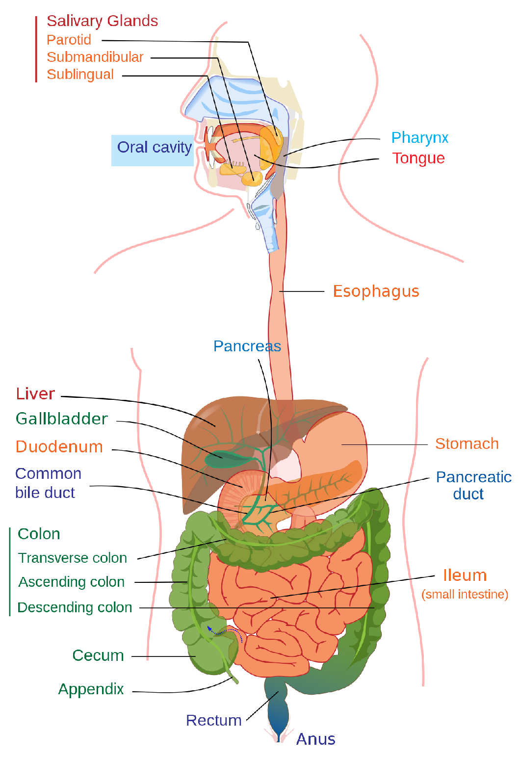
The human digestive system may be affected by several diseases. Any ailment that affects the digestive system is referred to as a digestive disease. Digestion disorders impact the gastrointestinal tract—sometimes referred to as the GI tract or the gastrointestinal system. The GI tract is made up of the stomach, large and small intestines, liver, pancreas and gallbladder (Figure 1).

The gastrointestinal (GI) tract is related to three of the eight most-prevalent malignancies. Approximately 2.8 million new cases and 1.8 million fatalities from colon, stomach and esophageal cancer occur each year [2]. The term “gastrointestinal cancer” describes cancerous disorders of the GI tract as well as the esophagus, stomach, biliary system, pancreas, small intestine, large intestine, rectum and anus. The signs and symptoms are related to the damaged organ and may include blockage (resulting in difficulties eating or urinating), abnormal bleeding or other related issues.

Overall, compared to other systems in the body, the GI tract and the supporting digestive organs (pancreas, liver and gall bladder) are the primary causes of cancer and cancer-related fatalities. Since 2020, nearly 27,600 general public in America have suffered from abdominal tumors, and 11,010 people are deceased [3]. The threat aspect of abdominal tumors is more advanced in men compared to women. Gastrointestinal polyps are abnormal tissue growths on the mucosa of the stomach and colon and are the source of gastrointestinal cancer. They develop slowly, and a person can feel the symptoms only when the polyps are huge. However, if discovered at an early stage, polyps can be avoided and treated.

Gastroscopy and colonoscopy are the two types of endoscopic examinations that play vital roles in the early detection of polyps in the GI tract and, thus, reduce the possible diseases [4]. While a colonoscopy checks the large intestine (colon) and rectum, a gastroscopy examines the upper GI tract, including the esophagus, stomach and first portion of the small bowel. Both of these tests include a real-time visual examination of the GI tract’s interior accomplished using digital high-definition endoscopes.

One of the newest medical imaging techniques for diagnosing gastrointestinal diseases, such as stomach ulcers, bleeding and polyps, is called wireless capsule endoscopy (WCE) [5]. A small wireless camera is used during a procedure called a capsule endoscopy to obtain images of the digestive system. The patient ingests a vitamin-sized capsule that contains an endoscopic camera. Thousands of photos are taken by the camera while the capsule passes through the digestive system, and they are sent to a recorder that the patient wears on a belt around their waist.

Doctors can view the interior of the small intestine with the use of capsule endoscopy, which is easier to access than more conventional endoscopic techniques. In traditional endoscopy, a long, flexible tube with a video camera is inserted down the patient’s throat or via the rectum. Usually, the endoscopy is completed in eight minutes on one patient. The numerous images produced by medical capsule endoscopy require a great deal of time for specialists to review. Approximately 56,000 frames are produced for an eight-minute examination. However, only a handful of them are significant, and the remaining frames are ignored.

It is difficult to identify contaminated frames from those 56,000 frames, and hence this selection of significant frames is a crucial task [6]. Specialists manually complete this laborious and time-consuming task. After choosing the crucial frames, a second study was conducted to categorize the frames in accordance with infections, such as polyps, ulcers and bleeding. Manual labeling of this kind always requires a skilled individual. This makes manual diagnosis challenging, and a poor diagnosis could result from the radiologist’s incompetence and other human factors.

The experts may differ in their classification of various endoscopic findings and severity assessments. Identification of disease level must be precise as it may affect the treatment and follow-up. Endoscopic examinations are resource-intensive and necessitate specialized people as well as costly technological equipment. To minimize disparities, enhance quality and make the most use of limited medical resources, the automatic detection, recognition and assessment of abnormal findings are likely to be beneficial.

In order to diagnose diseases without the aid of an expert, an automated computing system using WCE frames is required [7]. However, these systems struggle with difficulties, such as poor contrast and complicated background images for reliable recognition. A number of imaging techniques have evolved, including 3D imaging, narrow-band imaging (NBI), magnifying endoscopy (ME) and autofluorescence imaging (AFI).

Therefore, a computer-aided automatic approach would be valued for accurately analyzing tumors and for doing so in the early stages of cancer. This has been demonstrated to improve the efficacy and quality of gastroscopy in routine clinical practice, acting as a “third eye” for endoscopists. Due to ongoing advancements in algorithms, hardware performance, processing power and the gathering of numerous labeled endoscopic image datasets, deep-learning (DL) technology have recently greatly enhanced the performance of computer-aided diagnosis systems. Therefore, automatic GI illness classification is still a topic that has to be studied in order to improve lesion identification and classification accuracy.

This paper mainly contributes to providing a computer-aided classification method for gastrointestinal diseases using endoscopic images without any preprocessing steps or image enhancement process. In this paper, we propose a transfer-learning approach using an EfficientNetB0 pre-trained model, and we perform a wide range of experiments to validate the efficiency of the proposed model. In addition, we compare our results with other related contemporary approaches and demonstrate better results. We also highlight the region in the endoscopic image that contributes to disease classification using Grad-CAM.

The remainder of the paper is structured as follows: An overview of gastrointestinal disorders affecting the GI tract is provided in Section 2. The many state-of-the-art (SOTA) techniques are described in Section 3. The methods and materials needed to diagnose a dataset are covered in Section 4. The analysis and study findings are reported in Section 5 along with comparisons between the proposed system and findings from other investigations. Section 6 presents our conclusions.

2. An Overview of Digestive Diseases

2.1. Cecum

The largest bowel’s closest portion is called the cecum. Reaching the cecum provides evidence that a colonoscopy has been completed, and this completion rate has proven to be a reliable quality measure for colonoscopies [8]. Therefore, it is crucial to recognize and record the cecum. The appendiceal aperture is one of the traits that identify the cecum. When identified or photographed in the reports, this—together with a typical configuration on the electromagnetic scope tracking system—may be utilized as evidence for cecum intubation [9]. The appendiceal orifice is depicted as a crescent-shaped slit in Figure 2, and the scope configuration for the cecal position is shown in green in Figure 2.

2.2. Pylorus

The region around the passage from the stomach into the first segment of the small bowel (duodenum) is referred to as the pylorus. Circumferential muscles in the aperture regulate the passage of food out of the stomach. One of the more difficult techniques in gastroscopy—endoscopic instrumentation to the duodenum—requires the identification of the pylorus. In order to detect certain conditions, such as ulcerations, erosions or stenosis, a thorough gastroscopy includes an examination on both sides of the pyloric aperture. An endoscopic view of a healthy pylorus as seen from inside the stomach is shown in Figure 2g. The smooth, round aperture may be seen in this image as a black circle surrounded by uniformly colored stomach mucosa.

2.3. Z Line

The gastro-esophageal junction, which marks the transition between the stratified squamous epithelium in the esophagus and the intestinal epithelium of the gastric cardia, is known as the Z line in the esophagus (the squamocolumnar junction). Although the Z line is a typical result, not all studies show it. Although the real danger of this finding is debatable, an irregular or raised Z line signals probable distal esophageal metaplasia/Barrett esophagus.

2.4. Ulcerative Colitis

The large bowel is affected by ulcerative colitis, a chronic inflammatory condition. The diagnosis is mostly based on colonoscopic findings, and the condition may have a significant impact on the quality of life. There are four levels of inflammation: none, mild, moderate and severe—each having a unique endoscopic profile. For instance, swollen and red mucosa is a sign of a mild condition, whereas ulcerations are more noticeable in a moderate case. Figure 2e depicts a case of ulcerative colitis with mucosal bleeding, edema and ulceration. Fibrin, which is white in the image, covers the wounds. An automatic computer-aided evaluation method can help to grade the disease severity more accurately.

2.5. Esophagitis

The esophagus will become inflamed with esophagitis. The mucosal lining and circular and longitudinal smooth muscle fibers make up the esophagus—a tube. Food and liquids often travel through it as it links the throat to the stomach. Esophagitis can be asymptomatic, or it can produce searing discomfort in the chest and/or abdomen, especially when lying down or straining, and it can make swallowing challenging (dysphagia). Acid reflux from the stomach into the lower esophagus is the most typical cause of esophagitis. If the condition is not addressed, it may result in esophageal pain and scarring. Esophagitis may lead to esophageal ulcers if the irritation is not given time to heal. Barrett’s esophagus can result from esophagitis, which also raises the risk of esophageal cancer.

2.6. Polyps

Polyps are intestinal lesions that may be identified by mucosal outgrows. A typical polyp is demonstrated in Figure 2f. The polyps may be identified from normal mucosa by color and surface pattern, and they can be flat, raised or pedunculated. The majority of intestinal polyps are benign; however, some might develop into cancer. In order to stop the growth of colorectal cancer, polyps must be found and removed. Automatic identification could enhance the quality of a checkup because doctors may ignore polyps. This aids in locating the endoscope tip’s present location (and, consequently, the location of the polyp) along the length of the colon during live endoscopy. For diagnosis, evaluation and reporting, automatic computer-assisted polyp identification would be beneficial.

2.7. Dyed Resection Margins

When determining whether or not the polyp has been entirely removed, the resection margins are crucial. Continued growth and, in the worst-case scenario, the development of cancer might result from residual polyp tissue. The resection location following a polyp-ectomy is shown in Figure 2d.

2.8. Dyed and Lifted Polyps

The injection of saline and indigo carmine was used to raise a polyp as seen in Figure 2a. Contrasted with the darker normal mucosa, the pale blue polyp borders are easily seen. The eventual presence of non-lifted regions might indicate malignancy.

3. Literature Review

Efficient assistance for pathological findings is offered by a computer-aided diagnostic system (CADx), which helps medical professionals to diagnose and identify anomalies. In the past, machine-learning models and, currently, deep-learning models are becoming vital players in spotting abnormalities in the GI tract.

Handcrafted features, such as color, texture and edge features, have been extracted from endoscopic images that rely on trial and error for disease diagnosis using machine-learning algorithms. Convolutional neural networks (CNNs) have started to address these feature engineering issues, and their use of supervised learning has significantly enhanced the ability to diagnose medical images. By applying engineering techniques to the learning process, CNNs have demonstrated an outstanding capacity to extract features [10]. Medical image diagnostics have been proven to beat expert performance using deep-learning systems. Therefore, computer-aided diagnosis for endoscopic imaging utilizing deep-learning algorithms has the potential to attain diagnostic accuracy that is superior to that of qualified specialists.

In order to diagnose colon polyps, Karkanis et al. [11] presented a method for obtaining color characteristics based on wavelet decomposition. In numerous studies, authors have used machine-learning techniques to extract features from gastrointestinal images using edge shape and valley information, polyp-based local binary, gray-level co-occurrence matrices (GLCMs), wavelets and context-based features [12,13,14].

In [15], gemstone spectrum imaging was employed to analyze lymph node metastases in gastric cancer utilizing machine-learning techniques. With 38 lymph node samples from gastric cancer, they utilized the kNN classifier to differentiate lymph node metastasis from non-lymph node metastasis, achieving a global accuracy of 96.33% after utilizing feature selection and metric knowledge approach to minimize data dimension and feature space.

Wang Y et al. [16] devised a system for colonoscopy polyp detection. Throughout the colonoscopy, this system can provide an alarm with a real-time reaction. To recognize polyp boundaries, the authors employed visual fundamentals and a rule-based classifier. For polyp finding, the system attained an accuracy of 97.7%.

A CNN approach for detecting polyps from CT colonography images was presented by Godkhindi and Gowda [17]. Their algorithm isolates the colon from the other organs by segmenting it from the CT image. The colon polyp is subsequently identified by extracting the form features. Ozawa et al. [18] described a method for Single Shot MultiBox Detector (SSD)-based colorectal polyp detection and reported encouraging diagnostic outcomes. A two-stage polyp segmentation and automated classification system were presented by Pozdeev et al. [19]. The presence or absence of a tumor is classified in the first stage using the overall characteristics of endoscopic images, and CNN segmentation is used in the second step.

By extracting color information from lesions, Min et al. [20] created a computer-aided approach to diagnose linked color imaging. The technique successfully distinguished between adenomatous polyps and non-adenomatous polyps in pictures. In addition, Song et al. [21] used CNN techniques to establish a computer-aided approach for classifying colorectal polyp histology into three categories: serrated polyp, deep submucosal cancer and benign adenoma mucosal or superficial submucosal cancer.

Segu et al. [22] proposed a detailed CNN technique to describe small intestinal motion. This CNN-based strategy made use of the overall depiction of six separate abdominal motility events by mining deep features, which resulted in superior classification performance when compared to the other handmade feature-based approaches. Despite achieving a high classification score of 96% accuracy, they only considered a small number of classes.

Gamage et al. [23] employed pre-trained DenseNet-201, ResNet-18 and VGG-16 CNN prototypes as feature extractors with a universal average pooling (GAP) layer to produce a collection of deep features as the only feature vector with a probability correctness of 97.38%. The suggested technique predicted only eight different types of digestive tract abnormalities. In this paper, we propose a transfer-learning model that enhances the prediction accuracy of GI tract diseases.

Sutton et al. [24] used CNN techniques to clearly discriminate patients with ulcerative colitis from non-ulcerative colitis and to show the endoscopic disease severity. Yogapriya et al. [25] studied the GI tract disease classification using VGG16, ResNet-18 and GoogLeNet models and reported 96.33% accuracy with VGG-16.

4. Experimental Setup

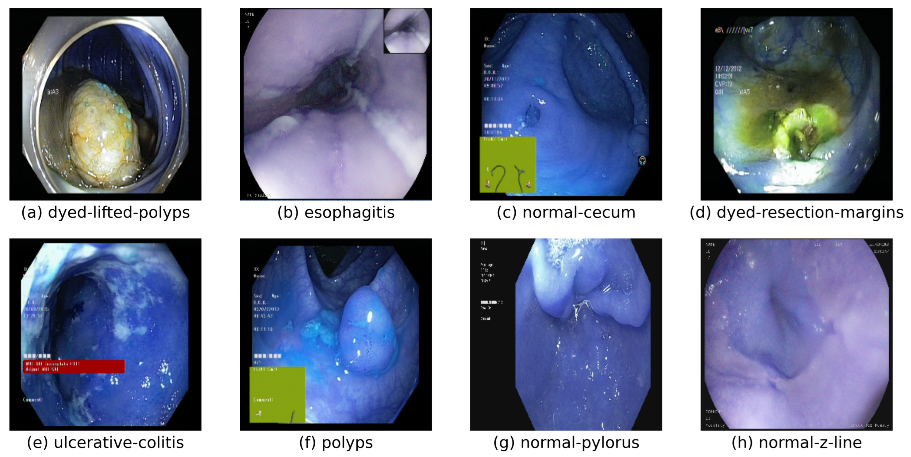
The entire experiment was conducted using an openly accessible multi-class KVASIR dataset [26]. A significant number of images are available in the dataset to employ in a variety of tasks, including image retrieval, machine learning, deep learning and transfer learning. The collection includes 8000 expert-verified images of anatomical landmarks, pathological findings and endoscopic operations in the GI tract for eight distinct digestive diseases. The Z line, pylorus and cecum are anatomical markers, whereas esophagitis, polyps and ulcerative colitis are pathological findings.

The images in the dataset range in resolution from 720 × 576 to 1920 × 1072 pixels, and they are grouped with names that correspond to the contents of the images. The position and configuration of the endoscope inside the intestine are shown in some of the image classes and presented as a green picture-in-picture taken using an electromagnetic imaging system (ScopeGuide, Olympus Europe), which may aid in the interpretation of the image. In this paper, we considered five diseases—dyed lifted polyps, normal cecum, normal pylorus, polyps and ulcerative colitis—for the classification task.

A total of 5000 images for the five diseases with each disease consisting of 1000 images were considered for the experiment. For the classification task, the dataset was split into training, validation and test sets in the ratio of 80%, 10% and 10%, respectively. For the custom CNN, 100 epochs were considered while transfer-learning approaches attained better results in 10 epochs.

4.1. CNN and Transfer Learning

In this study, we conducted two experiments: custom deep CNN and transfer learning (TL) using pre-trained CNN models with the KVASIR image dataset. We did not employ any preprocessing or augmentation techniques. We utilized Google Tensorflow as the backend for all deep-learning implementations, together with Keras, and the implementation was conducted using a MacBook M1 Air with 16GB RAM. We created a custom CNN, with five convolutional layers, trained from scratch.

The rectified linear unit (ReLU) and maxpooling were utilized as the activation function and pooling function, respectively. The final classification phase was performed using two dense layers with ReLU and Sigmoid acting as the activation functions with a 0.5 dropout inserted in each layer. We used the Adam optimizer, and the custom CNN was trained with 100 epochs. The hyperparameters used are shown in

Table 1. The model hyperparameters.

Custom CNN Layers	FC Layers	Batch Size	Optimizers	Activations	Dropout
5	2	64	Adam	ReLu + Softmax	0.25

.

A model created for one task being used as the basis for another using the machine-learning technique is known as transfer learning. This method can train deep neural networks with relatively minimal data, making it quite popular in deep learning. It can occasionally take days or even weeks to train a deep neural network from scratch on a challenging problem; therefore, transfer learning decreases training time as well. In this paper, we use four popular DL models as the base model for TL: ResNet50, InceptionV3, DenseNet121 and EfficientNetB0. A brief overview of each model is given below.

4.2. ResNet50

A 50-layer convolutional neural network called ResNet50 has 48 convolutional layers, one MaxPool layer and one average pool layer. Deep networks are challenging to train because of the well-known vanishing gradient problem in which the gradient becomes increasingly small as it is repeatedly multiplied and back-propagated to older layers. Due to this, with a deeper network, its performance becomes saturated or even starts to decline quickly. ResNet uses skip connections to transfer the output from one layer to another. This aids in reducing the issue of the vanishing gradient. The ResNet50 model uses a bottleneck design for its building block. A “bottleneck” residual block employs 1 × 1 convolutions to minimize the number of parameters and matrix multiplications. Each layer’s training can now be completed much more quickly.

4.3. InceptionV3

A convolutional neural network design from the Inception family called InceptionV3 includes a number of advances, such as the inclusion of an auxiliary classifier to transport label information lower down the network, factorized 7 × 7 convolutions and employing label smoothing. The InceptionV3 model incorporates several changes, such as factorization of larger convolutions into smaller convolutions, spatial factorization into asymmetric convolutions, usage of auxiliary classifiers and reduction of the grid size, resulting in an architecture made up of 42 layers. Compared to its predecessors and its contemporaries, the InceptionV3 model has an incredibly low error rate and high-performance efficiency.

4.4. DenseNet121

As stated earlier, when the number of layers increases or becomes deeper, the vanishing gradient problem arises. By altering the typical CNN design and streamlining the connection pattern across layers, DenseNet alleviates this issue. Each layer in a DenseNet design is directly linked to every other layer—thus, the term densely connected convolutional network. There are $L(L+1)/2$ direct connections for layers of length ‘L’. A total of 120 convolutions and four AvgPool make up DenseNet121. All layers, including transition layers and those in the same dense block, distribute their weights over several inputs, enabling deeper layers to leverage features that were extracted earlier. In comparison to the normal CNN or ResNet equivalents, DenseNets produce more compact models because they require fewer parameters and permit feature reuse. They have also achieved state-of-the-art performances and superior outcomes across competing datasets.

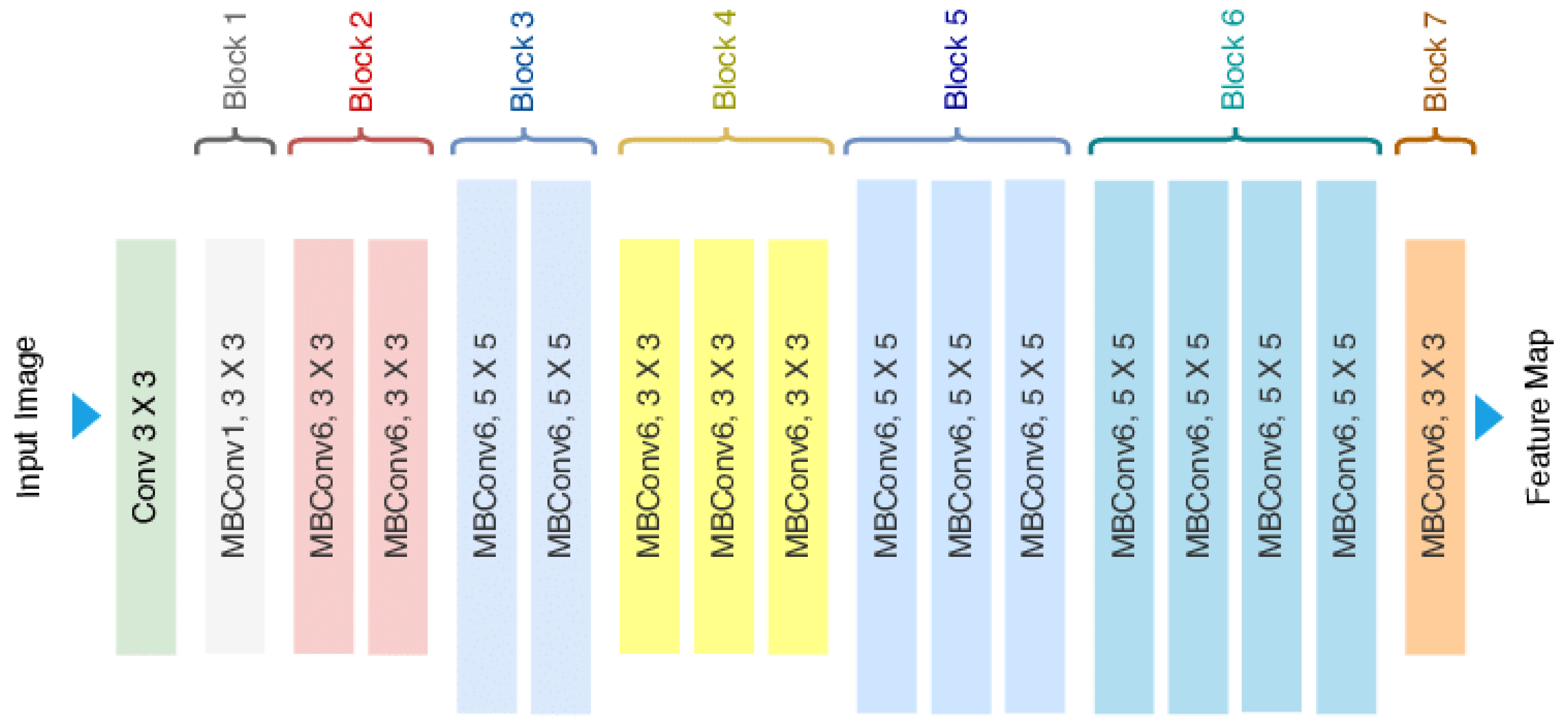
4.5. EfficientNetB0

In order to increase the effectiveness of an existing ConvNet based on the available resources, EfficientNet is a CNN that employs a scaling technique called compound scaling (memory and FLOPS). The mobile inverted bottleneck MBConv combined with an added Squeeze and Excitation (SE) block forms the basis of the EfficientNetB0 model. The MBConv uses Depthwise Separable Convolution, i.e., first, the channels will be widened by a point-wise convolution (conv $1\times 1$) and a $3\times 3$ depth-wise convolution that significantly reduces the number of parameters. Finally, it uses a $1\times 1$ convolution to reduce the number of channels. Dynamic feature channel-wise recalibration is a method in which the network dynamically allocates high weight to the most relevant channels, rather than assigning equal weight to all of the channels. CNNs increase the inter-dependencies between the channels using an SE block, which uses the dynamic feature channel-wise recalibration techniques. The architecture of EfficientNetB0 is shown in Figure 3. The resulting networks outperformed numerous state-of-the-art networks in terms of both efficiency and performance.

Generally, convolution is performed in the lower layers of the CNN. The feature maps of the final convolution layer are vectorized and input to the fully connected layers followed by a softmax logistic layer. Thus, the convolution layers act as feature extractors, and these features are used for classification. Overfitting is more likely to occur in fully connected layers, which reduces the network’s capacity for generalization. In this article, we propose to use global average pooling in place of fully connected layers.

With global average pooling, the average of each feature map is calculated and the resulting feature vector is input directly into the softmax layer. This strategy offers several advantages. First, overfitting is avoided because the global average pooling layer has no parameters to optimize. Secondly, it enforces correspondences between feature maps and categories, making it more natural to the convolution structure. Thus, it is simple to interpret the feature maps as category confidence maps. Another advantage is that global average pooling sums out the spatial information, and hence it is more robust to spatial translations of the input.

In all the experiments, a learning rate annealer was used. If the error rate does not change after a certain number of epochs, the learning rate annealer reduces the learning rate. Using this technique, we examined the validation accuracy and if there was a plateau in three epochs, it reduced the learning rate by 0.01.

5. Results and Discussion

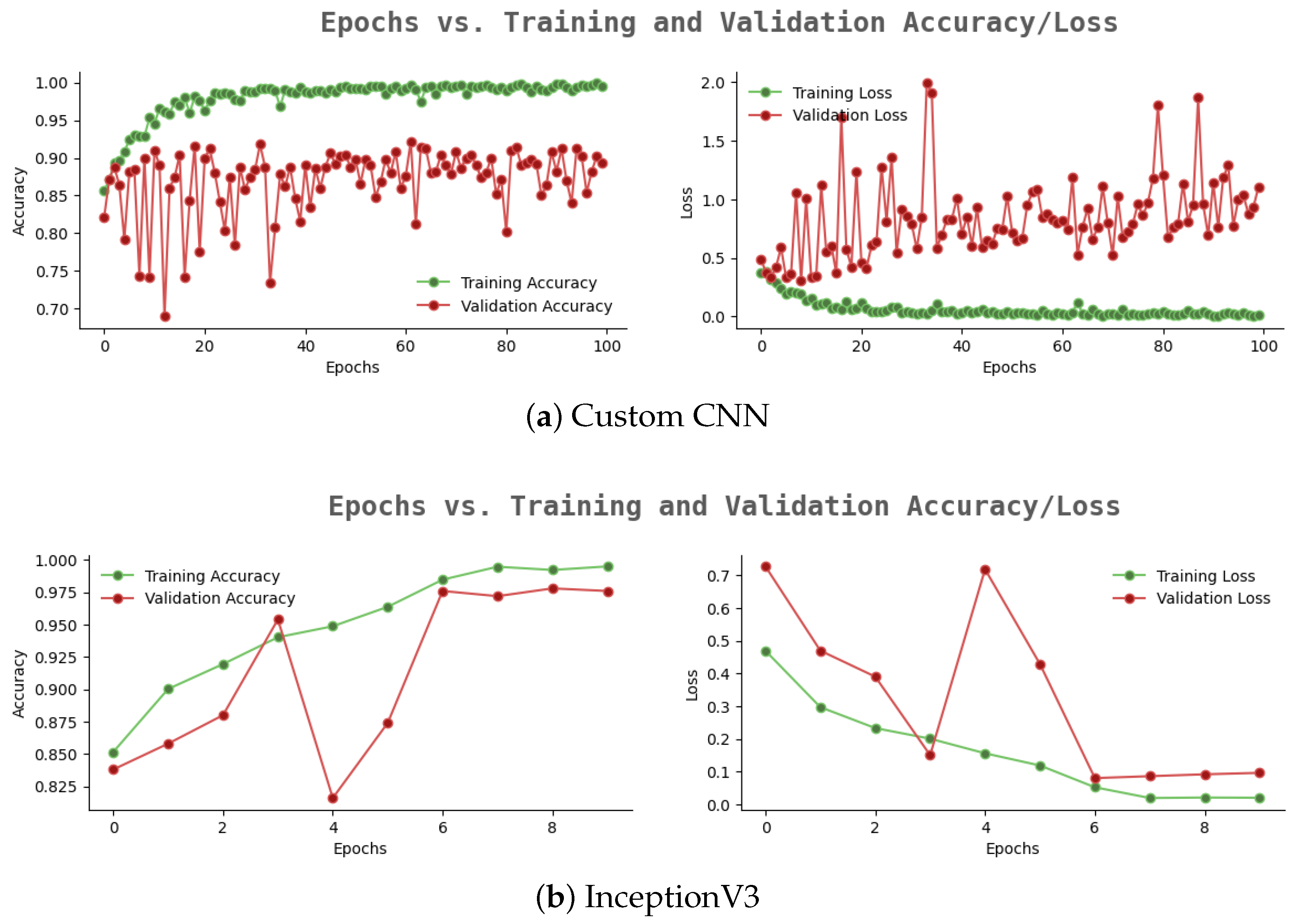
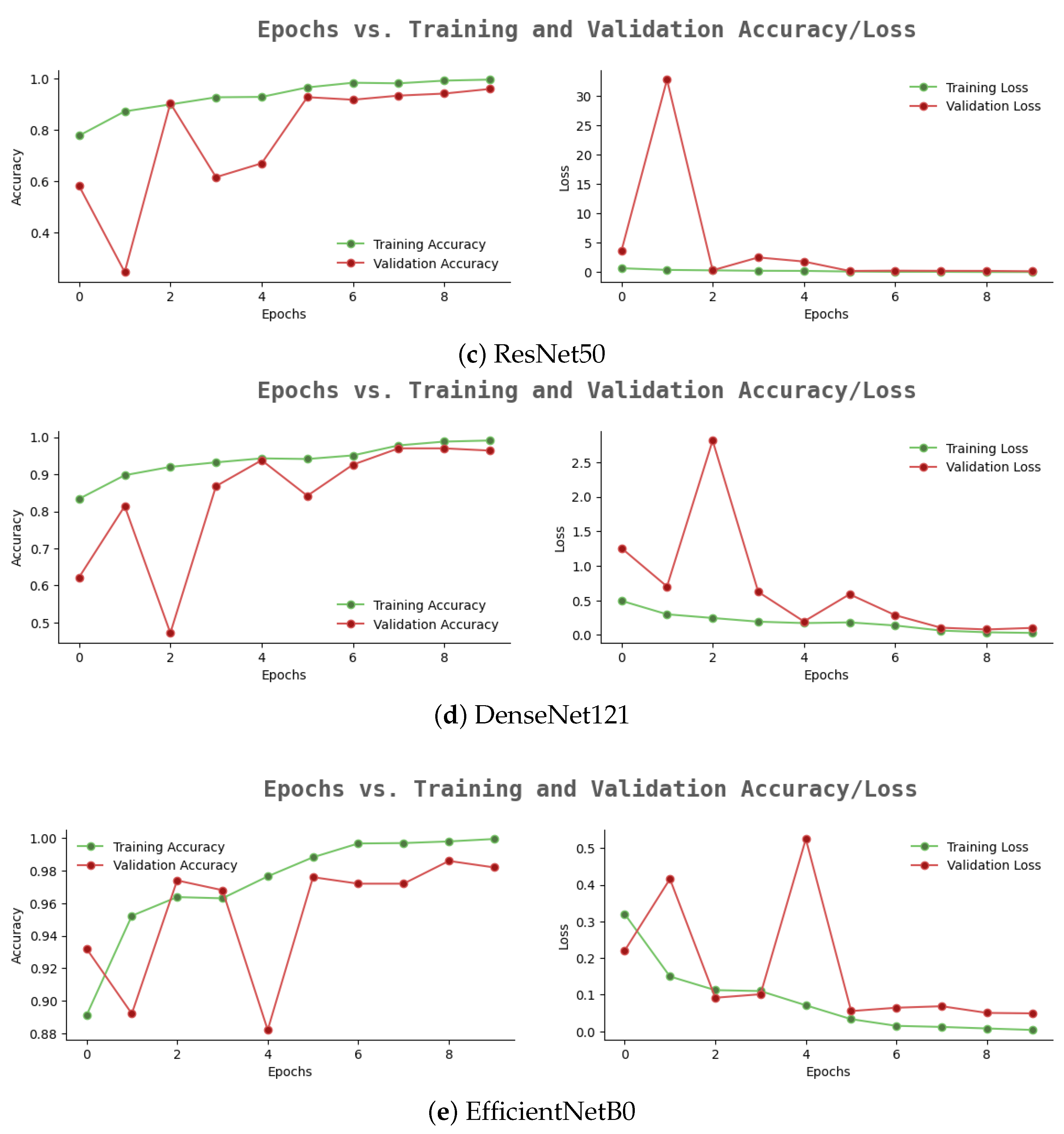
In this section, the performance accuracy and other metrics, such as the precision, recall and F1 score, obtained by our proposed CNN model and DL models using transfer learning are compared to the baseline system of the dataset developers and a number of other SOTA methods on the KVASIR dataset. The hyperparameter chosen is shown in Table 1, and the proposed model was trained and evaluated for 100 epochs. For the proposed CNN, the accuracy and loss on the training and validation dataset are shown in Figure 4a.

The custom CNN model resulted in 89% testing accuracy as shown in

Table 2. Results for the proposed custom CNN and transfer-learning models for five diseases.

Model	Accuracy	Precision	Recall
Custom CNN	89.04	89.01	89.00
TL + ResNet50 (Pre-trained)	95.00	95.00	95.00
TL + InceptionV3 (Pre-trained)	97.00	96.00	96.00
TL + DenseNet121 (Pre-trained)	97.00	96.00	95.00
TL + EfficientNetB0 (Pre-trained)	98.01	98.00	98.00

. We observed that the model suffers from an overfitting problem. In order to improve the performance accuracy and to avoid the overfitting problem, we used a pre-trained deep-learning model (InceptionNet, ResNet, DenseNet and EfficientNet) as the basis and then retrained the model on the KVASIR disease dataset, i.e., transfer learning. Transfer learning improves the performance accuracy of the system. Figure 4b–e shows the accuracy and loss achieved on the training and validation dataset.

The training accuracy and validation accuracy are reported as 99.97%, 98.75% (ResNet), 99.5%, 97.8% (InceptionNet), 99.33% and 97% (DenseNet) and 99.97%, 98.75% (EfficientNet). It is abundantly evident that the overfitting issue is resolved by the transfer-learning method when used with these pre-trained models. Table 2 shows the test dataset evaluation for four TL models.

The proposed systems achieved precision of 95%, 96%, 96% and 98%; recall of 95%, 96%, 95% and 98%; and accuracy of 95%, 97%, 97% and 98.01% for ResNet50, InceptionV3, DenseNet121 and EfficientNetB0, respectively. The findings from each network were encouraging, and, among other pre-trained models, EfficientNetB0 achieved a superior accuracy of 98.01%, because of the deft depth, breadth and resolution scaling, thereby, outperforming other SOTA systems.

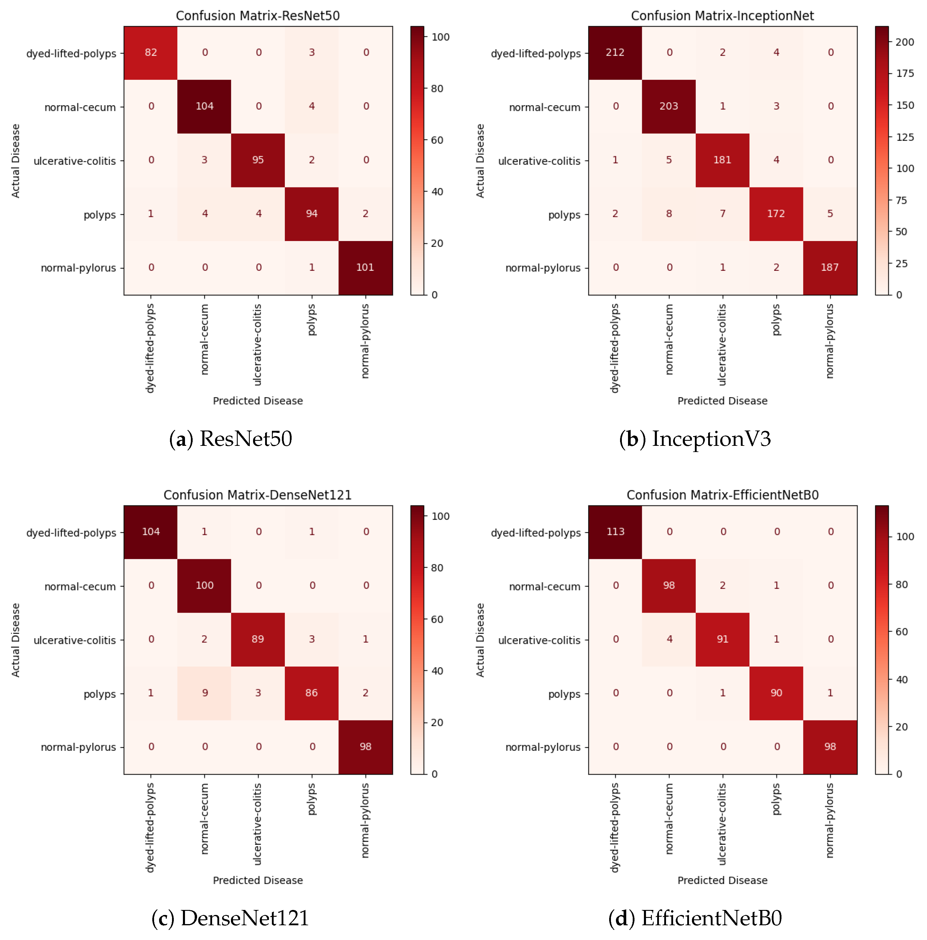
Confusion matrices shown in Figure 5 for the TL models indicate the identification accuracy for each of the individual diseases. The ResNet50 model had the maximum prediction accuracy for the normal-pylorus disease (101 out of 102 samples). The DenseNet121 models performed well in predicting normal-cecum and normal-pylorus diseases with 100% accuracy. The EfficientNetB0 model achieved 100% prediction accuracy for normal-pylorus and dyed lifted polyps and 99% prediction accuracy for polyp disease. It also achieved better results compared with the other pre-trained models considering other metrics, such as the precision, recall and F1-score.

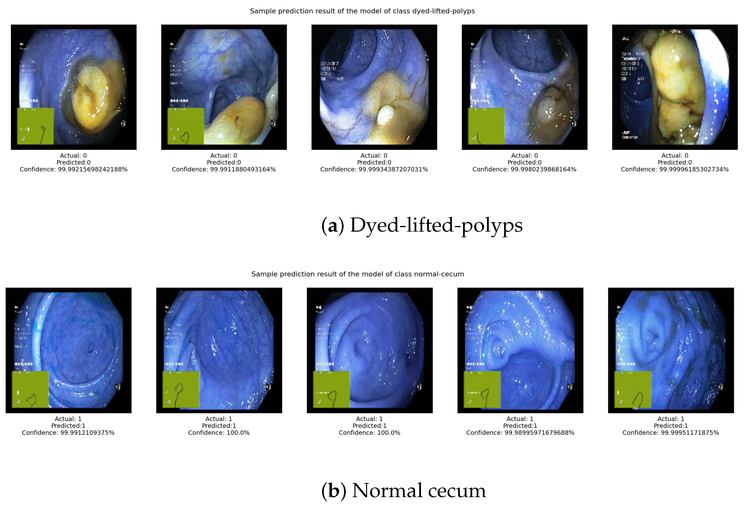
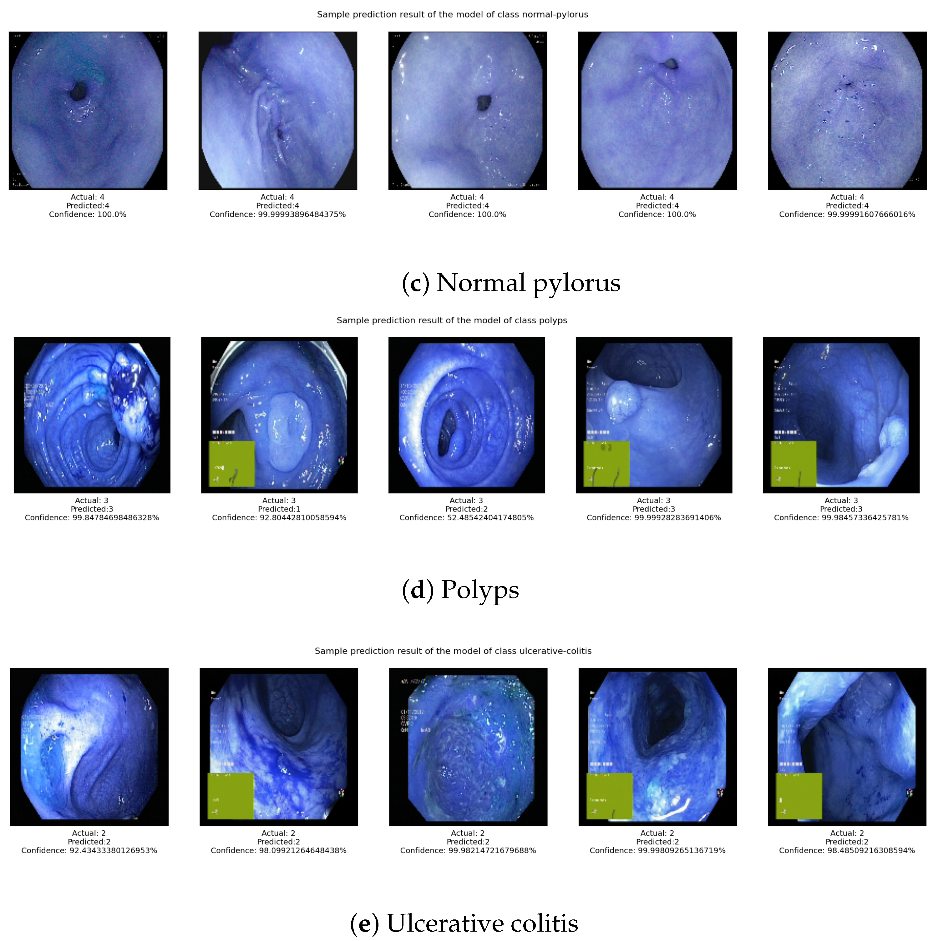
Figure 6 shows the actual disease and predicted disease for the transfer-learning model using EfficientNetB0. It can be seen that the actual disease and predicted disease are the same in almost all cases.

Table 3. Comparison of the identification accuracy of our proposed system with other SOTA models.

Model	Accuracy
Godkhindi and Gowda [17]	88.56
Pozdeev et al. [19]	88.00
Ribeiro et al. [28]	90.96
Fonolla et al. [29]	90.20
Mosleh Hmoud et al. [27]	97.00
Proposed model (custom CNN)	89.04
Proposed model (ResNet50)	95.00
Proposed model (InceptionV3)	97.00
Proposed model (DenseNet121)	97.00
Proposed model (EfficientNetB0)	98.01

shows the accuracy of the proposed approaches compared with other contemporary methods. While Mosleh Hmoud Al-Adhaileh et al. reported 97% testing accuracy [27], the proposed TL approach using the ResNet50 model’s accuracy was less than the SOTA method. The proposed TL using the InceptionV3 and DenseNet121 models performed equally to the SOTA systems. Interestingly, the EfficientNetB0 model surpassed the SOTA systems, and its identification accuracy was 98.01%. It is to be noted that we did not perform any image preprocessing or image augmentation techniques as in other systems, but were still able to obtain better identification accuracy.

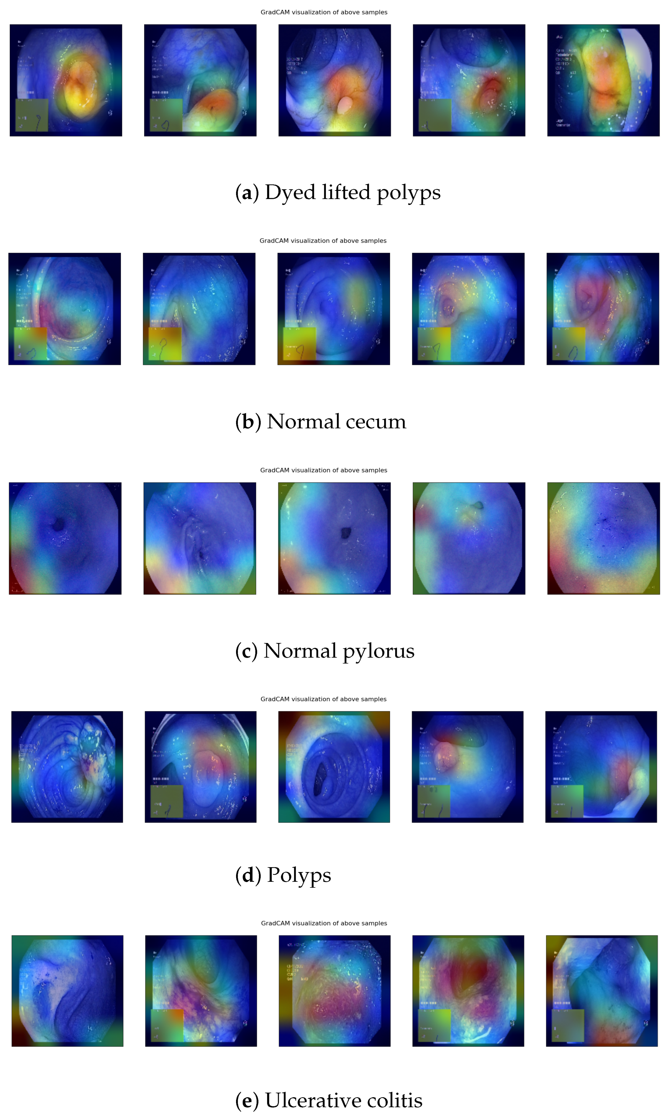
Visualization of Outputs

Grad-CAM is a method for increasing the transparency of convolutional neural network (CNN)-based models by highlighting the input regions that are vital for the models’ predictions or visual explanations. Using a gradient class activation map to visualize CNN’s final layers makes it easier to identify the area of the image that CNN needs for classification. Figure 7 shows the Grad-CAM visualization of the same sample images belonging to the five different diseases shown in Figure 6.

The Grad-CAM images were generated for the sample images taken from the test dataset that were predicted correctly. It can be observed that the Grad-CAM highlights the infected regions in red color as these are medically relevant. In other words, the regions that are in red contribute the maximum activation in classifying the image, while the regions in blue have no activation. This provides some support to the claim that the model is able to focus on the regions of the image that are medically relevant in identifying digestive diseases.

6. Conclusions

In this paper, we examined endoscopy images of digestive systems and proposed a transfer-learning model to improve the performance of the automated classification tool in diagnosing digestive diseases. The proposed system uses several pre-trained deep-learning models, including ResNet50, InceptionV3, DenseNet121 and EfficientNetB0. All the models performed well and achieved equal values for all the performance metrics. Among the four, the EfficientNetB0 model achieved the maximum performance results of 98.01% accuracy and 98% precision, recall and F1-score—a slight increase in performance compared to the other state-of-the-art systems. In the future, using various medical images, the suggested technique may be utilized to detect or diagnose a number of additional disorders. By using image-enhancing techniques, we can still improve the performance results.