Article

A Novel Approach for Data Feature Weighting Using Correlation Coefficients and Min–Max Normalization

Center for Artificial Intelligence Technology, Faculty of Information Science and Technology, Universiti Kebangsaan Malaysia (UKM), Bangi 43600, Selangor, Malaysia
*
Author to whom correspondence should be addressed.
Symmetry 2023, 15(12), 2185; https://doi.org/10.3390/sym15122185
Submission received: 16 October 2023 / Revised: 27 November 2023 / Accepted: 1 December 2023 / Published: 11 December 2023
(This article belongs to the Topic Decision-Making and Data Mining for Sustainable Computing)

Abstract

:
In the realm of data analysis and machine learning, achieving an optimal balance of feature importance, known as feature weighting, plays a pivotal role, especially when considering the nuanced interplay between the symmetry of data distribution and the need to assign differential weights to individual features. Also, avoiding the dominance of large-scale traits is essential in data preparation. This step makes choosing an effective normalization approach one of the most challenging aspects of machine learning. In addition to normalization, feature weighting is another strategy to deal with the importance of the different features. One of the strategies to measure the dependency of features is the correlation coefficient. The correlation between features shows the relationship strength between the features. The integration of the normalization method with feature weighting in data transformation for classification has not been extensively studied. The goal is to improve the accuracy of classification methods by striking a balance between the normalization step and assigning greater importance to features with a strong relation to the class feature. To achieve this, we combine Min–Max normalization and weight the features by increasing their values based on their correlation coefficients with the class feature. This paper presents a proposed Correlation Coefficient with Min–Max Weighted (CCMMW) approach. The data being normalized depends on their correlation with the class feature. Logistic regression, support vector machine, k-nearest neighbor, neural network, and naive Bayesian classifiers were used to evaluate the proposed method. Twenty UCI Machine Learning Repository and Kaggle datasets with numerical values were also used in this study. The empirical results showed that the proposed CCMMW significantly improves the classification performance through support vector machine, logistic regression, and neural network classifiers in most datasets.

1. Introduction

Data preprocessing is one of the most crucial steps in machine learning. Using important and necessary methods to prepare raw data correctly will positively affect the output and improve a model’s performance [1,2]. The data preparation stage includes many tasks, such as removing outliers and noise, integrating data from diverse sources, dealing with missing data, and transforming data into a scale suitable for analysis. This stage aims to eliminate the impact of systematic sources of variation as much as is feasible [3,4]. While data scaling is considered a treatment for domination issues in most cases, it will have a reverse impact when giving the same contribution to a feature that is irrelevant to the target feature. In this case, using feature weighting to select essential features is one of the solutions, and using it to balance a feature based on its importance is the other possible solution. In many data-mining algorithms, such as neural network algorithms, clustering, and distance-based algorithms, data rescaling is an essential stage prior to the training phase to avoid misleading results and speed up the learning process [5,6,7]. To avoid numeric features dominating other numeric values, transforming all feature values into a standard range will give equal importance to all features [4,6]. Many research findings suggest that data normalization and standardization substantially impact classification and clustering results [8]. The effect of data normalization on the results of many machine learning (ML) methods has been studied, such as its effect on classification accuracy [9,10], neural network training [11,12], the clustering process [8], and outlier detection methods [13]. When data have been normalized, all features have an equal contribution to ML results, but it does not mean that these features are equally important. In some cases, data have many irrelevant and redundant features. Ref. [14] proposed the Adaptive Distinct Feature Normalization Strategy, which enhances the fusion of sparse topics and deep features by adaptively normalizing them separately. This results in a clearer feature description and decreases confusion in complex scenes. The presence of undesired features makes learning difficult and increases the feature’s space. Generally, normalization gives all features the same contribution to a model. But removing any dominant features may reduce the model’s performance. In this case, the behavior of data plays a vital role in the performance [15].
In the same context, feature weighting is one of the essential stages since it is used to adjust the feature values based on their contribution to the model and the result [16]. Many variable importance measurements are presented and categorized into sub-categories based on the techniques used. One of those techniques is the correlation coefficient, a parametric regression technique. Another different strategy is the nonparametric strategy which includes multiple techniques; one example is Random Forest [17]. Many researchers have used variable importance measurement strategies and applied them to enhance the classifier’s performance, such as [18], naive Bayes text classifiers [19,20], the fuzzy clustering method, and feature weighting used for the neural network [21,22], with SVMs [23]. Also, feature weighting has been used as a feature selection strategy to know the influence of features on results and then exclude irrelevant, redundant features [24,25,26], as well as the information gain attribute [27].
In contrast, a correlation coefficient is a measurement tool used to look for relationship patterns between different characteristics [28]. Therefore, a bivariate study measures the degree of association between two variables and the direction of the relationship [29]. In this context, the correlation coefficient can be considered as a variable importance method amongst parametric regression techniques when used to indicate linear dependence [17]. Various types of correlation coefficient formulas have been presented depending on the data type (numerical, ordinal, or nominal) and the type of correlation (linear or non-linear relationship) [30]. Pearson’s correlation coefficient is a measurement method to explore the linearity of a correlation [31] for numerical data only. Although the correlation coefficient has been used mainly in statistical analysis to discover relationships among variables, there are many other uses for correlation metrics, especially in data mining. For example, correlation coefficients have been used for feature selection [32,33,34], missing data imputation methods [35,36,37], and feature quality measurement to find the best splitting features and points of decision trees [38].
Normalization is a preprocessing step applied to data to give features equal importance and prevent the domination of a few features. The impact of normalization methods has been studied in many works [39,40,41]. The Min–Max normalization method is one of the best normalization methods that has been found to improve the performance of classifiers [42,43]. Data standardization has also produced better outcomes in neural network training, though the benefit decreases with increasing network and sample sizes [11]. Choosing the appropriate normalization method is essential, as it affects the performance of supervised learning algorithms [44]. Also, Ref. [40] examined the impact of four normalization techniques on forecasting. They found that standardization calculations have a high affectability, and that a cautious approach is needed to deal with the outcomes. The impact of normalization on the performance of different methods such as outlier detection, violent video classification, backpropagation neural networks, and classification performance has been studied, and it was found that the performance of normalization depends on both the data and the technique used [13,45]. Due to the importance of normalization, [46] proposed a new normalization method to only deal with integer values. The authors of [47] proposed two normalization methods, a “new approach to Min-Max” and a “new approach to Decimal Scaling,” to reduce the impact of large feature values and represent them in a small range. These methods are based on the Min–Max and Decimal Scaling normalization techniques. The study performed well with the k-means clustering method, but only that method was used for evaluation.
At the same time, feature weighting is another best strategy to prepare data to improve a method’s accuracy. Feature weighting methods are strategies for correlation analysis and dimension reduction, where the weight represents the contribution of each feature dimension to classification [48]. Ref. [49] proposed feature weighting methods based on similarity calculations using k-means, fuzzy c-means, and mean shift clustering. The weight of each feature is obtained by calculating the difference between original data and cluster centers, dividing by the mean of differences, and multiplying by the feature value in the dataset.
Ref. [50] proposed a support vector machine (SVM) with an information gain approach to improve fraud detection accuracy in card transactions. The approach involves normalizing the data using Min–Max normalization and reducing features through information gain-based feature selection. Discretization is carried out before normalization. Ref. [51] proposed a two-stage strategy combining normalization and supervised feature weighting using the Pearson correlation coefficient (PCC) and Random Forest Feature Importance estimation. The first stage involves normalizing the data using standardization. In contrast, the second stage involves calculating feature weights through the PCC and Random Forest Feature Importance and multiplying each feature value by weight. Ref. [52] proposed a dynamic feature-weighting algorithm to address multi-label classification by minimizing an objective function to bring together samples with the same label and separate samples with different labels. The weight function is used to evaluate the method with a multi-label classifier. Ref. [53] proposed a Correlation-Based Hierarchical k-Nearest Neighbor Imputation (CoHiKNN) method that weights the distance based on the correlation between the features and the label. The correlation coefficient is used to weigh the distance and impute missing values using k-NN. The weighting strategy multiplies each difference between two points by the correlation coefficient value of the feature. Ref. [54] proposed a hybrid data-scaling method combining Min–Max and Cox-Box to improve fault classification performance in compressors. The Min–Max method rescales data to one range, while Cox-Box transforms non-linear distributions into normal ones.
However, although it is essential to normalize the data and give all features the same contribution to override the feature’s dominance over the results of the model, in many cases, the importance of variables varies from one feature to another. Also, normalization has some limitations, such as destroying the original structure of the dataset [50]. In addition, using the feature weight for selecting important features has some limitations, in that the selected features still have an equal contribution. Also, using a subset of the dataset can decrease the quality and results of the correlation coefficient due to low instance numbers, affecting the correct weight assigned to each feature [53].
In this work, we tried to balance the importance of normalization with the various importance of features and reduce feature domination by employing data standardization, as well as maximizing the feature contribution by maximizing the value based on its correlation coefficient. The maximization limit parameter is proposed to control the new range of feature values. We investigate the influence of normalization on the classification and regression methods using three data types in two phases. First, we implement the un-normalized data (raw data) and normalized data using one normalization method. In the second phase, the normalized data are used to weight the values depending on the association among the values with the class feature. This step calculates the correlation coefficient between the class feature and the rest of the features. This step increases the contribution of each feature based on its relationship with the class. Each value will increase based on its correlation, where features with higher correlation will experience a greater increase compared to features with lower correlation. This weighting strategy significantly influences the model construction, directing more attention towards features exhibiting high correlation. The features with strong correlation will potentially increase the model’s accuracy and achieve more power in classification algorithms.

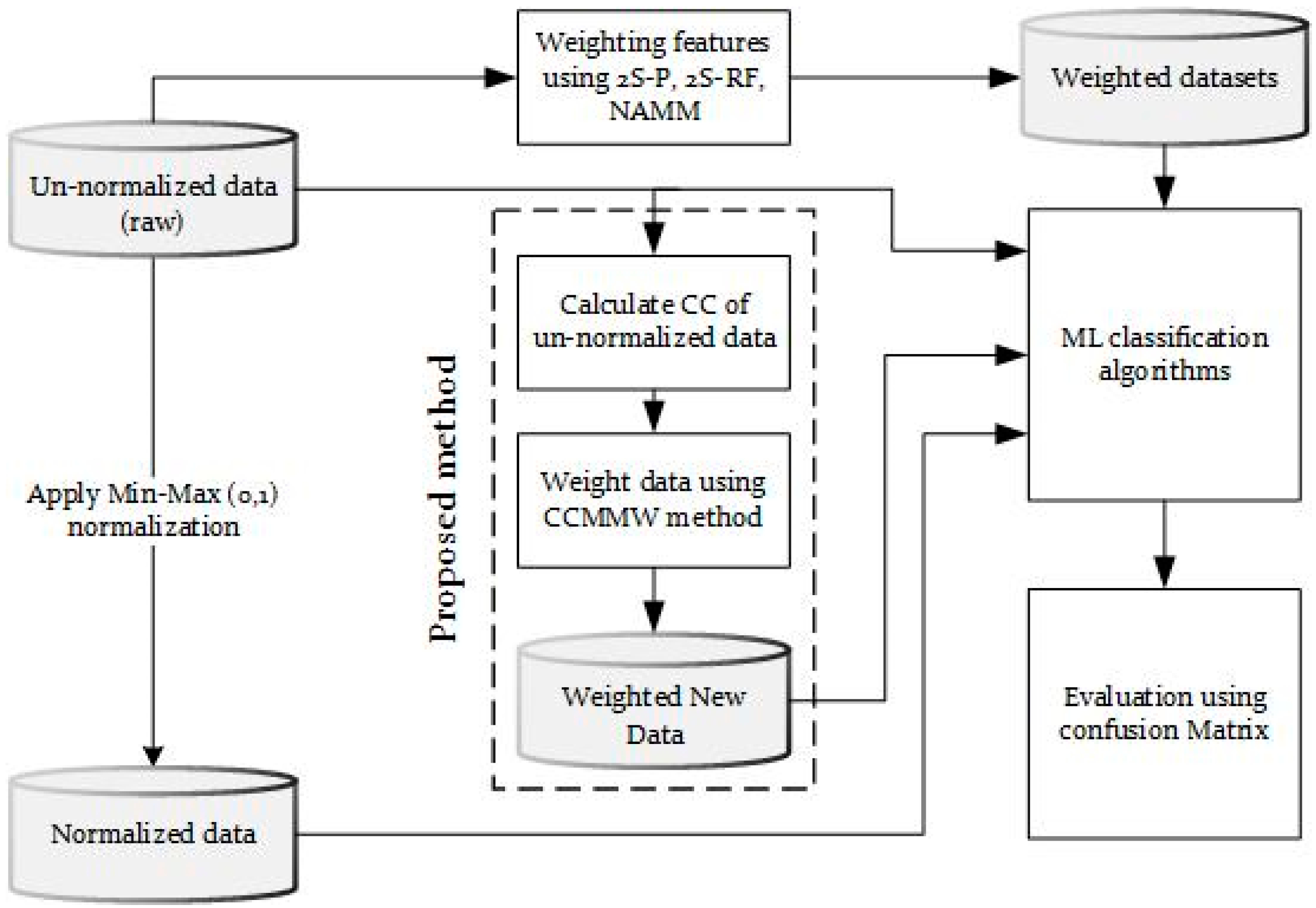
2. Materials and Methods

A new weighting strategy is proposed using the correlation value between features for data representation. The new data representation values are used to increase the contribution of data. Each value will be maximized depending on the feature’s actual value and Pearson correlation coefficient. Calculating the correlation between the class and the rest of the features is the initial step for weighting the feature values. The new maximum values will be calculated based on the actual and correlation coefficient values. First, all features will be normalized using Min–Max (0,1) to give the same contribution to all features, then increase the values using its correlation coefficient. The ensuing maximization step carefully calculates new maximum values by considering both the original feature values and their corresponding correlation coefficients. This dual-factor approach ensures that the augmented values strike a balance between the inherent importance of features and their contextual significance, enhancing the robustness of the data representation methodology. The strategy’s dual consideration of raw feature values and correlation coefficients establishes a nuanced approach that not only maximizes the impact of each feature but also captures the intricacies of their relationships within the dataset.
As the Min–Max (0,1) normalization method represents all features in the same range (0–1), the proposed method will modify this concept, where each feature will have its own range. If we assume that f1 is a feature with 0 correlation, all the values will represent the same value due to having no correlation with the class label. On the other hand, the features with a correlation of 1 with the class label will represent the new maximum value. The maximum value is determined based on the coefficient of change (C) and the correlation R-value. The relationship is direct between the coefficient of change and the maximum value, indicating that as the coefficient increases, the maximum value also increases, and vice versa. The maximum possible value for each feature corresponds to the correlation value of 1 (strong correlation) for that feature. In this scenario, strong correlation is the only case where new values can attain the maximum values.

Datasets and Experiments

The proposed method will calculate the correlation among features using the Pearson correlation coefficient (PCC) (Equation (1)) and Min–Max normalization (MMN) (Equation (2)). n e w _ m i n and n e w _ m a x denote the updated range of feature values, with n e w _ m i n set to 0 and n e w _ m a x set to 1 in the context of Min–Max scaling (0,1). The new weighted value is created using Equation (3).
r = i = 1 m ( x i x ¯ ) ( y i y ¯ ) i = 1 m ( x i x ¯ ) 2 i = 1 m ( y i y ¯ ) 2 .
M M N , x i , n = x i , n m i n ( x i ) max x i m i n ( x i ) n e w _ M a x n e w _ M i n + n e w _ M i n .
N e w   w e i g h t e d   v a l u e , v                                                 = V i , j m i j m a j m i j n e w _ m a x n e w _ m i n + n e w _ m i n                                                 + C V i , j m i j m a j m i j n e w _ m a x n e w _ m i n + n e w _ m i n . C o r r V j , V t a r g e t .
where the following are defined in Table 1:
The following, Algorithm 1 explains the steps of the proposed method CCMMW.
Algorithm 1 CCMMW algorithm
Algorithm: Normalization + Weighting data using Min-Max01 and CC
to improve the accuracy of classification methods
Input: Un-Data: un-normalize data
Output: CCoT Correlation Coefficient of Label feature, Normalized data (No-Data), Correlation Weighted
Normalized Data (CCMMW-Data)
CCoT = Calculate the correlation coefficient of each feature with the Label feature corr(Vj,VTarget) using
the PCC method as in Equation (1)
Calculate No-Data using MMN normalization method, Equation (2)
For i = 1 to n 1 , where n is the number of features in the data
     Calculate CCMMW-Data using the proposed method as in Equation (3)
Assume a dataset (D) with six features (F1 to F6) where D is the normalized Min–Max (0,1) data. As a result of the MMN method, each small value of features is presented as 0, and the maximum value is presented as 1, as in the original normalized Min–Max 0,1 data in Table 2. Also, the correlation among the complete dataset is shown in Table 3, where each correlation coefficient (CC) value represents the correlation coefficient value between the feature and the class label feature. Table 2 shows three sets of values as the results of CCMMW. The first is CCMMW(1), where the table is produced with a C parameter value of 1. Also, CCMMW(5) is produced using the CCMMW method with a value of 5 for the C parameter. Finally, CCMMW(10) is the results of the CCMMW method using a value of 10 for the C parameter.
As shown in Figure 1, the algorithm aims to improve the accuracy of classification methods by applying normalization and correlation-based weighting techniques to the input data. It starts by calculating the correlation coefficient between each feature and the target feature using the PCC method. Then, it normalizes the data using the Min–Max method to scale the values between 0 and 1. Next, it calculates the correlation-weighted normalized data for each feature, incorporating the correlation coefficients obtained. The algorithm outputs the correlation coefficient of the target feature, the normalized data, and the correlation-weighted normalized data. By normalizing the data and incorporating feature–target correlations, the algorithm aims to enhance the classification accuracy by giving more importance to relevant features in the classification process.
The general research methodology is presented in Figure 1; two strategies are used to transform the data prior to new data creation. One is transformed using existing and new approaches to normalization methods. The second uses CC values to weigh the features for representing the data, and then uses the new data to improve the accuracy of classification approaches. Then, the performance of the proposed method is compared using un-normalized and normalized data with different classifiers.
Experiments were conducted on twenty datasets comprising both discrete and continuous features to assess the proposed method’s consistency. These datasets were carefully selected from reputable sources, including the Machine Learning Repository UCI and Kaggle Repository databases. These databases are renowned for their diverse and well-curated datasets, making them valuable resources for empirical studies in this field. Table 4 provides an overview of the datasets. Also, various data sizes are considered, where various instances and features are used in the study.
In this experiment, to analyze the effect of weighting features based on its CC on the classification results, comparisons are made between the un-normalized (RAW) data, the normalized Min–Max (0,1) (MM) method, the Two-Stage Min–Max with Pearson (2S-P) method, the Two-Stage Min–Max with RF Feature Importance (2S-RF) method, the New Approach Min–Max Normalization method (NAMM), and the proposed CCMMW approach. All codes are written in Python 3.7. Jupyter (Anaconda 3). The SciKitLearn Library was used to implement all methods in this study. Five classification methods were used to investigate the impact on the performance and the improvement of the proposed method. The classifiers are the logistic regression (LR), SVM, k-nearest neighbor (kNN), neural network (NN), and naive Bayes (NB) classifiers. Finally, all experimental results were performed on numerical datasets.
In the evaluation stage, the effect of using the CC to weigh the normalized values was evaluated based on the type of algorithm that was applied to the data. For classification purposes, the result was evaluated based on the accuracy rate. Ten cross-validations and the experiment were repeated ten times, and the results were averaged for further analysis. For the k-NN classifier, 3 neighbors were considered as k values. In the kernel function of the SVM, RBF was used as the kernel parameter value, and all other settings used the default values.

3. Results

3.1. The Evaluation of Different Classifiers Based on the Best Result of CCMMW

The best results of CCMMW from 10 available values in the experiment results are shown in Figure 2. The ten results were due to the setting of the C parameter, which we used to adjust the new range of data. The impact of the various values of C is discussed in the further section of this discussion.
In the following results, the classification accuracy is presented. Bold values are the highest out of the six methods, and the CCMMW values are underlined when the value is the highest value after the raw values.

3.2. Logistic Regression (LR) Classifier

Table 5 shows that the CCMMW method obtained the highest accuracy in 12 out of the 20 datasets, and an extra four datasets if the raw data are excluded. It shows that the best accuracy improvement using the CCMMW + LR classifier compared with the MM method was 5.46%, obtained from the Letter dataset. The accuracy of MM was 71.46%, whereas CCMMW gave 76.92%. Although this case had the best raw data accuracy, the proposed method was still better than the other strategies. Also, the accuracy decreased in three cases out of twenty, whereas the worst was −1.24%.
As in Figure 2a, we find that, through a comparison between the proposed method and the MM normalization method, the proposed method excelled in most cases, as it excelled with 17 databases in this study, while MM excelled in only three cases, with an outperformance that did not exceed 1.24%. In addition, 2S-P outperformed in three cases while CCMMW outperformed in 17 cases, with a high difference in the Letter dataset, where 2S-P was 49.96% while CCMMW was 76.92%. Also, when comparing the results with 2S-RF, we find that, the same as with 2S-F, the proposed method outperformed 2S-RF with 17 datasets. In comparison, only 2S-RF outperforms in the Breast Cancer 1, German, and Blood datasets. The last compared method is the NAMM, where the proposed method performed well in all datasets except German, where the NAMM result was 73.53% while that of CCMMW was 72.56%. Only three differences between the NAMM and CCMMW had a less than 1% improvement, while all other results obtained were between 1.27 and 26.78% with Spam and Letter.

3.3. Support Vector Machine Classifier

Table 6 shows that CCMMW obtained the highest accuracy in 16 out of the 20 datasets, and an extra four datasets when raw data are excluded, when using model building based on weighting correlation features. When comparing CCMMW + SVM with the MM normalization method, as in Figure 2b, all the CCMMW results outperformed the MM results. The minimum increase was obtained with the German dataset, which was 0.38%, while the best result obtained was with Breast Ca Coimbra, which increased by 19.64%. Also, CCMMW outperformed 2S-P with all datasets. Some large differences were observed, such as 76.22%, 50.15%, 43.50%, and 27.49% with the Letter, Vehicle, Ecoli, and Sonar datasets, due to the bad performance of 2S-P with the SVM. The same was observed with 2S-RF, where some large differences in accuracy were obtained compared with CCMMW. Also, due to the bad performance of 2S-RF with the SVM, the difference reached 77.12% with the Letter dataset. The lower difference obtained with 2S-RF was 0.49%. Finally, compared with the NAMM, all CCMMW results outperformed the NAMM results. Overall, CCMMW+SVM outperformed the other data preparation methods, increasing the accuracy compared with the rest of the normalization and feature weighting methods. The significant results obtained from all datasets showed an improvement in accuracy. Only the raw data and CCMMW produced the best results with all datasets. The performance of CCMMW with the SVM increased significantly, such as 19.64%, 14.24%, 11.97%, and 11.18 with Breast Ca Coimbra, Vehicle, PARKINSON, and Monkey, respectively.

3.4. k-Nearest Neighbor (k-NN) Classifier

Table 7 shows that CCMMW obtained the highest accuracy in only two out of the 20 datasets, and an extra two datasets if the raw data are excluded. As shown in Table 7 and Figure 2c, the performance of CCMMW with the k-NN classifier compared with MM shows us that CCMMW was only improved with the QSAR, Liver, Breast Ca Coimbra, and Bupa datasets. The accuracy of other datasets obtained by CCMMW was less than the accuracy of MM. Also, compared to 2S-P and 2S-RF, CCMMW only outperformed six and eight datasets, respectively. The NAMM was the only method that CCMMW outperformed, whereas the proposed method outperformed in 14 out of 20 datasets.
Overall, the two improvements of the CCMMW + k-NN classifier were with the Breast Ca Coimbra dataset, while the improvement with QSAR was 0.91%. Another two improvements compared with the other methods (except for the raw data) were the liver and Bupa datasets, which reached 3.72% and 3.63% improvement, respectively. As seen in Figure 2c, the performance of CCMMW with the k-NN method had no improvement in general, where the results obtained by CCMMW were the worst when comparing most numbers.

3.5. Neural Network (NN) Classifier

The first thing we figured out from Figure 2d is that the raw data did not produce any of the best values in all datasets. Also, Table 8 show that Improvements were obtained with most of the datasets, where the accuracy increased with 15 datasets. The best improvement when using CCMMW with the NN classifier was 9.91% with the Letter dataset, while the second-best improvement was with Breast Ca Coimbra. The worst decrease with the NN classifier was 7.30%, where the accuracy decreased from 84.91% to 77.61%. Also, compared with the 2S-P method, the results show that CCMMW outperformed 2S-P, whereas, with 16 datasets, CCMMW produced higher accuracy than 2S-P. As with 2S-P, the comparison between 2S-RF and CCMMW favored the proposed method as it also outperformed when applied to most of the datasets. Although the NAMM outperformed CCMMW in three datasets (Monkey: 2.62% higher; Hearts Cleveland: 0.24% higher; and Blood: 0.32% higher), CCMMW performed as expected with the rest of the datasets. Some of the performance differences were high, such as 24% higher with Wholesale, 23.78% with Sonar, and 22.39% with Vehicle. Overall, we can conclude that CCMMW performed better when applied to data when using the NN classifier.

3.6. Naive Bayes Classifier

Table 9 shows that CCMMW obtained the highest accuracy in 10 out of the 20 datasets. Compared with the rest of the normalization and raw methods, as in Figure 2e, CCMMW produced high accuracy, outperforming others. Ten datasets were given high accuracy when using CCMMW with the NB classifier, while MM exceeded with only two datasets: Wine and Magic. The best accuracy increase for CCMMW with the NBC was 2.44% with Blood. Weighting features using 2S-P produced higher accuracy than CCMMW with eight datasets, while 2S-RF outperformed with eleven datasets. The same happened with the NAMM, which obtained the two best accuracies overall, 97.86% with the Musk dataset and 79.86% with the Glass dataset.

4. Discussion

For an overall discussion, we calculated the average accuracy of the methods with the twenty datasets.
As shown in Figure 3, the average accuracy is presented as an indicator of the accuracy results on various datasets. Also, Table 10 shows the average accuracy in numbers. the Logistic regression outperformed other preparation methods, where it had the best results in 12 out of the 20 datasets, and an extra four results outperformed other methods, except for the raw data. In the second method, the SVM classifier shows a clear improvement in accuracy when using the CCMMW strategy. Out of the 20 datasets, 16 gave the best accuracy with the SVM. In comparison, an extra four datasets gave the best accuracy when raw data are excluded. For the k-NN classifier, the proposed method’s accuracy was slightly lower than the others. For the NN classifier, the results still show a good improvement in the accuracy of CCMMW. In 15 out of 20 datasets, its accuracy outperformed the other methods. Finally, although the averaged results present the proposed method as the fourth-best result, this is in part due to a lower difference between the results, where its accuracy with 11 datasets outperforms all other methods.

The Effect of C Parameter on the CCMMW Results

As we see in Figure 4a–e and Figure 5a–e, the primary role of parameter C is to adjust the range of the data, since the relationship between C and the maximum value of the new range is direct, so the range increases as the value of C increases.
As we see in Figure 4a, the best results of CCMMW were obtained with a high C value of 10. Most of the best results were obtained with C values of more than 5, as in Figure 4a (around 80%). Only three of the best results were obtained with C values less than 5, meaning that increasing the range of values by increasing the C parameter values will positively impact the results with the LR classifier. Like LR, CCMMW with a high C parameter value gave good results with the SVM classifier. As shown in Figure 4b, most of the best results with the SVM were obtained specifically with a C value of 10, which is 67% of the result, as shown in Figure 5b. Only with the German and Wholesale datasets was the best accuracy result reached with a C value of 1. In some cases, multiple C values obtained the same result. All results of the SVM show that increasing the C parameter’s value positively impacted the classifier’s results, where all results showed increasing accuracy. Although the results of CCMMW with the k-NN classifier did not outperform other classifiers, where it is considered as having a weak impact on the results among the classifiers, the best results with CCMMW were obtained by setting a high C parameter value of 10, as seen in Figure 5c, where it represents 80% of the high results. All of the higher results were obtained with C values of 10, as seen in Figure 4c. In contrast to the previous methods, most of the good results of the proposed method were obtained by using a value of 5 or less for C, which is around 62% of the higher results, as seen in Figure 5d. Although some of the higher accuracies of CCMMW were obtained with C values greater than 5, the best results of the other methods with the NN were with C values less than 5. We can conclude that the impact of the C values on the NN were not clearly impactful, which means that adjusting the range towards higher possible values is not the best approach, as seen in Figure 4d. Figure 5e illustrates that higher accuracy was mostly achieved with small C values. For the naive Bayes (NB) model, the optimal result was obtained at C = 1, yielding 16%, whereas for C values of 2, 3, 4, and 5, the accuracy remained consistent at 12% each. This cumulative value amounts to 64% in total. According to the experimental results, data normalization has the potential to develop prediction models with the highest prediction accuracy. However, compared to the results of models with normalized and non-normalized data, the accuracy was improved based on many factors such as the used normalization method, the type of data, and the classification methods.

5. Conclusions

Our experiment discusses the impact of the maximization of the role of features based on their correlation. The impact of the combined data normalization and feature weight is apparent. Although normalization impacted the results positively by giving an equal contribution of features to avoid eliminating features with high range values, the weighted features outperform those methods by increasing the contribution of the features based on the dependency measurement of features, such as the CC of importance of feature measurement. In this study, we have presented a novel feature weighting with normalization method named the Correlation Coefficient Min–Max Weighted (CCMMW) method. The relation between the correlation in the normalization area has not received much attention in the literature. We used the CC values to give features with a strong association more contribution to the learning step in ML methods to improve the performance of those methods. We used the LR, SVM, k-NN, NN, and NB classification methods to evaluate the effect of CCMMW. The performance improvement of the SVM, NN, and LR classifiers was clear, as most results showed increased accuracy. Only the k-NN classifier’s accuracy results were unsuitable, where the proposed method outperformed the Min–Max normalization method in 40% of the datasets. Still, other normalization and weighted methods outperform CCMMW in most cases. Also, adjusting the upper limit of the feature’s maximum value plays the main role in reaching the best result of the proposed method. In future work, various normalization methods could be explored, as each method offers distinct advantages that may impact the outcomes of data transformation. Additionally, incorporating alternative weight measurement methods may enhance the significance of features in constructing classification models, potentially leading to improved accuracy.

Author Contributions

Conceptualization, methodology, and software: M.S.; validation: M.S., Z.O. and A.A.B.; formal analysis, investigation, resources, data curation, and writing—original draft preparation: M.S.; writing—review and editing: Z.O. and A.A.B.; supervision: Z.O. and A.A.B.; funding acquisition: Z.O. All authors have read and agreed to the published version of the manuscript.

Funding

This work was funded in part by the Malaysian Ministry of Higher Education under the Fundamental Research Grant Scheme (FRGS): FRGS/1/2021/ICT06/UKM/02/1; The Faculty of Information Science and Technology, Universiti Kebangsaan Malaysia: FTM1 and Center for Artificial Intelligence Technology, Universiti Kebangsaan Malaysia: FTM3.

Data Availability Statement

The data presented in this study are openly available in Machine Learning Repository UCI and Kaggle Repository databases.

Acknowledgments

We would like to thank the Data Mining and Optimization Lab of the Faculty of Information Science and Technology, Universiti Kebangsaan Malaysia, for the expert knowledge sharing.

Conflicts of Interest

The authors declare no conflict of interest. The funders had no role in the design of the study; in the collection, analyses, or interpretation of data; in the writing of the manuscript; or in the decision to publish the results.

Abbreviations

The following abbreviations are used in this manuscript:
CCMMWCorrelation Coefficient with Min–Max Weighted
PCCPearson correlation coefficient
MMNMin–Max normalization
CCcorrelation coefficient
2S-PTwo-Stage Min–Max with Pearson
2S-RFTwo-Stage Min–Max with RF Feature Importance
NAMMNew Approach Min–Max
NBnaive Bayes
NNneural network
LRlogistic regression
kNNk-nearest neighbor

References

  1. Niño-Adan, I.; Manjarres, D.; Landa-Torres, I.; Portillo, E. Feature weighting methods: A review. Expert Syst. Appl. 2021, 184, 115424. [Google Scholar] [CrossRef]
  2. Han, T.; Xie, W.; Pei, Z. Semi-supervised adversarial discriminative learning approach for intelligent fault diagnosis of wind turbine. Inf. Sci. 2023, 648, 119496. [Google Scholar] [CrossRef]
  3. Muralidharan, K. A note on transformation, standardization and normalization. Int. J. Oper. Quant. Manag. 2010, IX, 116–122. [Google Scholar]
  4. García, S.; Luengo, J.; Herrera, F. Data Preprocessing in Data Mining; Springer: Cham, Switzerland, 2015; Volume 72. [Google Scholar]
  5. Mohamad Mohsin, M.F.; Hamdan, A.R.; Abu Bakar, A. The Effect of Normalization for Real Value Negative Selection Algorithm. In Soft Computing Applications and Intelligent Systems; Noah, S.A., Abdullah, A., Arshad, H., Abu Bakar, A., Othman, Z.A., Sahran, S., Omar, N., Othman, Z., Eds.; Springer: Berlin/Heidelberg, Germany, 2013; pp. 194–205. [Google Scholar]
  6. Han, J.; Kamber, M.; Pei, J. 3—Data Preprocessing. In Data Mining, 3rd ed.; Han, J., Kamber, M., Pei, J., Eds.; Morgan Kaufmann: Boston, MA, USA, 2012; pp. 83–124. [Google Scholar] [CrossRef]
  7. Cui, Y.; Wu, D.; Huang, J. Optimize TSK Fuzzy Systems for Classification Problems: Minibatch Gradient Descent With Uniform Regularization and Batch Normalization. IEEE Trans. Fuzzy Syst. 2020, 28, 3065–3075. [Google Scholar] [CrossRef]
  8. Trebuňa, P.; Halčinová, J.; Fil’o, M.; Markovič, J. The importance of normalization and standardization in the process of clustering. In Proceedings of the 2014 IEEE 12th International Symposium on Applied Machine Intelligence and Informatics (SAMI), Herl’any, Slovakia, 23–25 January 2014; pp. 381–385. [Google Scholar]
  9. Adeyemo, A.; Wimmer, H.; Powell, L.M. Effects of Normalization Techniques on Logistic Regression in Data Science. J. Inf. Syst. Appl. Res. 2019, 12, 37. [Google Scholar]
  10. Rajeswari, D.; Thangavel, K. The Performance of Data Normalization Techniques on Heart Disease Datasets. Int. J. Adv. Res. Eng. Technol. 2020, 11, 2350–2357. [Google Scholar]
  11. Shanker, M.; Hu, M.Y.; Hung, M.S. Effect of data standardization on neural network training. Omega 1996, 24, 385–397. [Google Scholar] [CrossRef]
  12. Yao, J.; Han, T. Data-driven lithium-ion batteries capacity estimation based on deep transfer learning using partial segment of charging/discharging data. Energy 2023, 271, 127033. [Google Scholar] [CrossRef]
  13. Kandanaarachchi, S.; Muñoz, M.A.; Hyndman, R.J.; Smith-Miles, K. On normalization and algorithm selection for unsupervised outlier detection. Data Min. Knowl. Discov. 2020, 34, 309–354. [Google Scholar] [CrossRef]
  14. Zhu, Q.; Zhong, Y.; Zhang, L.; Li, D. Adaptive Deep Sparse Semantic Modeling Framework for High Spatial Resolution Image Scene Classification. IEEE Trans. Geosci. Remote Sens. 2018, 56, 6180–6195. [Google Scholar] [CrossRef]
  15. Singh, D.; Singh, B. Investigating the impact of data normalization on classification performance. Appl. Soft Comput. 2020, 97, 105524. [Google Scholar] [CrossRef]
  16. Dialameh, M.; Jahromi, M.Z. A general feature-weighting function for classification problems. Expert Syst. Appl. 2017, 72, 177–188. [Google Scholar] [CrossRef]
  17. Wei, P.; Lu, Z.; Song, J. Variable importance analysis: A comprehensive review. Reliab. Eng. Syst. Saf. 2015, 142, 399–432. [Google Scholar] [CrossRef]
  18. Zhang, L.; Jiang, L.; Li, C.; Kong, G. Two feature weighting approaches for naive Bayes text classifiers. Knowl.-Based Syst. 2016, 100, 137–144. [Google Scholar] [CrossRef]
  19. Nataliani, Y.; Yang, M.-S. Feature-Weighted Fuzzy K-Modes Clustering. In Proceedings of the 2019 3rd International Conference on Intelligent Systems, Metaheuristics & Swarm Intelligence, Male, Maldives, 23–24 March 2019; pp. 63–68. [Google Scholar]
  20. Malarvizhi, K.; Amshakala, K. Feature Linkage Weight Based Feature Reduction using Fuzzy Clustering Method. J. Intell. Fuzzy Syst. 2021, 40, 4563–4572. [Google Scholar] [CrossRef]
  21. Zeng, X.; Martinez, T.R. Feature weighting using neural networks. In Proceedings of the 2004 IEEE International Joint Conference on Neural Networks (IEEE Cat. No. 04CH37541), Budapest, Hungary, 25–29 July 2004; pp. 1327–1330. [Google Scholar]
  22. Dalwinder, S.; Birmohan, S.; Manpreet, K. Simultaneous feature weighting and parameter determination of neural networks using ant lion optimization for the classification of breast cancer. Biocybern. Biomed. Eng. 2020, 40, 337–351. [Google Scholar] [CrossRef]
  23. Zhang, Q.; Liu, D.; Fan, Z.; Lee, Y.; Li, Z. Feature and sample weighted support vector machine. In Knowledge Engineering and Management; Springer: Berlin/Heidelberg, Germany, 2011; pp. 365–371. [Google Scholar]
  24. Wang, J.; Wu, L.; Kong, J.; Li, Y.; Zhang, B. Maximum weight and minimum redundancy: A novel framework for feature subset selection. Pattern Recognit. 2013, 46, 1616–1627. [Google Scholar] [CrossRef]
  25. Wang, Y.; Feng, L. A new hybrid feature selection based on multi-filter weights and multi-feature weights. Appl. Intell. 2019, 49, 4033–4057. [Google Scholar] [CrossRef]
  26. Singh, D.; Singh, B. Hybridization of feature selection and feature weighting for high dimensional data. Appl. Intell. 2019, 49, 1580–1596. [Google Scholar] [CrossRef]
  27. Othman, Z.; Shan, S.W.; Yusoff, I.; Kee, C.P. Classification techniques for predicting graduate employability. Int. J. Adv. Sci. Eng. Inf. Technol. 2018, 8, 1712–1720. [Google Scholar] [CrossRef]
  28. Swesi, I.; Abu Bakar, A. Feature Clustering for PSO-Based Feature Construction on High-Dimensional Data. J. Inf. Commun. Technol. 2019, 18, 439–472. [Google Scholar] [CrossRef]
  29. Schober, P.; Boer, C.; Schwarte, L.A. Correlation coefficients: Appropriate use and interpretation. Anesth. Analg. 2018, 126, 1763–1768. [Google Scholar] [CrossRef] [PubMed]
  30. Khamis, H. Measures of association: How to choose? J. Diagn. Med. Sonogr. 2008, 24, 155–162. [Google Scholar] [CrossRef]
  31. Ratner, B. The correlation coefficient: Its values range between +1/−1, or do they? J. Target. Meas. Anal. Mark. 2009, 17, 139–142. [Google Scholar] [CrossRef]
  32. Hall, M.A. Correlation-Based Feature Selection of Discrete and Numeric Class Machine Learning; Department of Computer Science, University of Waikato: Hamilton, New Zealand, 2000. [Google Scholar]
  33. Saidi, R.; Bouaguel, W.; Essoussi, N. Hybrid Feature Selection Method Based on the Genetic Algorithm and Pearson Correlation Coefficient. In Machine Learning Paradigms: Theory and Application; Hassanien, A.E., Ed.; Springer International Publishing: Cham, Switzerland, 2019; pp. 3–24. [Google Scholar] [CrossRef]
  34. Hsu, H.-H.; Hsieh, C.-W. Feature Selection via Correlation Coefficient Clustering. J. Softw. 2010, 5, 1371–1377. [Google Scholar] [CrossRef]
  35. Rahman, G.; Islam, Z. A decision tree-based missing value imputation technique for data pre-processing. In Proceedings of the Ninth Australasian Data Mining Conference, Ballarat, Australia, 1–2 December 2011; pp. 41–50. [Google Scholar]
  36. Chen, X.; Wei, Z.; Li, Z.; Liang, J.; Cai, Y.; Zhang, B. Ensemble correlation-based low-rank matrix completion with applications to traffic data imputation. Knowl.-Based Syst. 2017, 132, 249–262. [Google Scholar] [CrossRef]
  37. Sefidian, A.M.; Daneshpour, N. Estimating missing data using novel correlation maximization based methods. Appl. Soft Comput. 2020, 91, 106249. [Google Scholar] [CrossRef]
  38. Mu, Y.; Liu, X.; Wang, L. A Pearson’s correlation coefficient based decision tree and its parallel implementation. Inf. Sci. 2018, 435, 40–58. [Google Scholar] [CrossRef]
  39. Pan, J.; Zhuang, Y.; Fong, S. The Impact of Data Normalization on Stock Market Prediction: Using SVM and Technical Indicators. In Soft Computing in Data Science; Berry, M.W., Mohamed, A.H., Yap, B.W., Eds.; Springer: Singapore, 2016; pp. 72–88. [Google Scholar]
  40. Kumari, B.; Swarnkar, T. Importance of data standardization methods on stock indices prediction accuracy. In Advanced Computing and Intelligent Engineering; Springer: Berlin/Heidelberg, Germany, 2020; pp. 309–318. [Google Scholar]
  41. Singh, D.; Singh, B. Effective and efficient classification of gastrointestinal lesions: Combining data preprocessing, feature weighting, and improved ant lion optimization. J. Ambient Intell. Humaniz. Comput. 2021, 12, 8683–8698. [Google Scholar] [CrossRef]
  42. Ali, N.A.; Omer, Z.M. Improving accuracy of missing data imputation in data mining. Kurd. J. Appl. Res. 2017, 2, 66–73. [Google Scholar] [CrossRef]
  43. Henderi, H.; Wahyuningsih, T.; Rahwanto, E. Comparison of Min-Max normalization and Z-Score Normalization in the K-nearest neighbor (kNN) Algorithm to Test the Accuracy of Types of Breast Cancer. Int. J. Inform. Inf. Syst. 2021, 4, 13–20. [Google Scholar] [CrossRef]
  44. Shahriyari, L. Effect of normalization methods on the performance of supervised learning algorithms applied to HTSeq-FPKM-UQ data sets: 7SK RNA expression as a predictor of survival in patients with colon adenocarcinoma. Brief. Bioinform. 2017, 20, 985–994. [Google Scholar] [CrossRef] [PubMed]
  45. Jayalakshmi, T.; Santhakumaran, A. Statistical normalization and back propagation for classification. Int. J. Comput. Theory Eng. 2011, 3, 1793–8201. [Google Scholar]
  46. Patro, S.; Sahu, K.K. Normalization: A preprocessing stage. arXiv 2015, arXiv:1503.06462. [Google Scholar] [CrossRef]
  47. Dalatu, P.I.; Midi, H. New Approaches to Normalization Techniques to Enhance K-Means Clustering Algorithm. Malays. J. Math. Sci. 2020, 14, 41–62. [Google Scholar]
  48. Jin, D.; Yang, M.; Qin, Z.; Peng, J.; Ying, S. A Weighting Method for Feature Dimension by Semisupervised Learning With Entropy. IEEE Trans. Neural Netw. Learn. Syst. 2023, 34, 1218–1227. [Google Scholar] [CrossRef]
  49. Polat, K.; Sentürk, U. A novel ML approach to prediction of breast cancer: Combining of mad normalization, KMC based feature weighting and AdaBoostM1 classifier. In Proceedings of the 2018 2nd International Symposium on Multidisciplinary Studies and Innovative Technologies (ISMSIT), Ankara, Turkey, 19–21 October 2018; pp. 1–4. [Google Scholar]
  50. Poongodi, K.; Kumar, D. Support vector machine with information gain based classification for credit card fraud detection system. Int. Arab J. Inf. Technol. 2021, 18, 199–207. [Google Scholar]
  51. Niño-Adan, I.; Landa-Torres, I.; Portillo, E.; Manjarres, D. Analysis and Application of Normalization Methods with Supervised Feature Weighting to Improve K-means Accuracy. In Proceedings of the 14th International Conference on Soft Computing Models in Industrial and Environmental Applications (SOCO 2019), Seville, Spain, 13–15 May 2019; Martínez Álvarez, F., Troncoso Lora, A., Sáez Muñoz, J.A., Quintián, H., Corchado, E., Eds.; Springer International Publishing: Cham, Switzerland, 2020; pp. 14–24. [Google Scholar]
  52. Dialameh, M.; Hamzeh, A. Dynamic feature weighting for multi-label classification problems. Prog. Artif. Intell. 2021, 10, 283–295. [Google Scholar] [CrossRef]
  53. Liu, X.; Lai, X.; Zhang, L. A Hierarchical Missing Value Imputation Method by Correlation-Based K-Nearest Neighbors. In Intelligent Systems and Applications: Proceedings of the 2019 Intelligent Systems Conference (IntelliSys), London, UK, 5–6 September 2019; Springer: Cham, Switzerland, 2019; pp. 486–496. [Google Scholar]
  54. Kim, S.-i.; Noh, Y.; Kang, Y.-J.; Park, S.; Lee, J.-W.; Chin, S.-W. Hybrid data-scaling method for fault classification of compressors. Measurement 2022, 201, 111619. [Google Scholar] [CrossRef]
Figure 1. The general CCMMW methodology.
Symmetry 15 02185 g001
Figure 2. The CCMMW performance on different classifiers. (a) LR. (b) SVM. (c) k-NN. (d) NN. (e) NB.
Symmetry 15 02185 g002aSymmetry 15 02185 g002b
Figure 3. CCMMW performance: average accuracy (20 datasets) of five classification methods (classifiers).
Symmetry 15 02185 g003
Figure 4. The value of C. (a) LR. (b) SVM. (c) k-NN. (d) NN. (e) NB.
Symmetry 15 02185 g004
Figure 5. Value range of C. (a) LR. (b) SVM. (c) k-NN. (d) NN. (e) NB.
Symmetry 15 02185 g005
Table 1. Definition of parameters in Equation (3).
v the new weighted value m i j Minimum value of column j
V i , j each original value m a j Maximum value of column j
C the parameter to adjust the new range n e w _ m i n New minimum value (0)
C o r r V j , V t a r g e t the correlation coefficient among column j and column label using PCC n e w _ m a x New maximum value (1)
Table 2. CC values among features and the label feature using the proposed weight feature.
Original Normalized Min–Max (0,1) DataCCMMW (1)CCMMW (5)CCMMW (10)
F1F2F3F4F5F6F1F2F3F4F5F6F1F2F3F4F5F6F1F2F3F4F5F6
0.000.000.000.000.000.000.000.000.000.000.000.000.000.000.000.000.000.000.000.000.000.000.000.00
0.250.250.250.250.250.250.250.280.310.380.450.500.250.380.560.881.251.500.250.500.881.502.252.75
0.500.500.500.500.500.500.500.550.630.750.901.000.500.751.131.752.503.000.501.001.753.004.505.50
0.750.750.750.750.750.750.750.830.941.131.351.500.751.131.692.633.754.500.751.502.634.506.758.25
1.001.001.001.001.001.001.001.101.251.501.802.001.001.502.253.505.006.001.002.003.506.009.0011.00
Table 3. CC among features and the label feature.
FeatureF1F2F3F4F5F6
CC value0.000.100.250.500.801.00
Table 4. Experiment datasets.
DatasetsType of Data# of Instances# of Features# Classes
Breast Cancer 1 real569302
QSAR real1055412
Sonar real208602
PARKINSON real195222
Wine Integer + real6463122
Monkey Integer55662
German real1000242
Musk Integer65981662
liver Integer + real34562
wholesale Integer44082
Spam real4601572
Heart s Cleveland Integer + real1190112
Magic real19,020102
Blood Integer74842
Breast Cancer Coimbra real11692
Vehicle Integer846184
Bupa Integer + real34562
Glass real21496
Letter Integer20,0001626
Ecoli real33678
Table 5. Performance of CCMMW on logistic regression classifier.
DatasetRAWMM2S-P2S-RFNAMMCCMMW
Breast Cancer 1 93.2997.0597.7397.2994.9796.89
QSAR 88.1187.4685.6984.6186.3387.75
Sonar 82.1679.4273.1974.0280.3283.56
PARKINSON 84.1388.3582.0881.5886.9891.27
Wine 98.8299.2598.8798.9394.6699.47
Monkey 91.8890.6474.5582.5989.3491.50
German 73.8272.3576.6676.2073.5372.56
Musk 94.3399.1293.1892.3890.2699.27
liver 65.3369.1762.2663.9157.9870.85
wholesale 84.9890.7590.5990.6167.7391.14
Spam 94.1093.4792.7292.8692.4193.68
Heart s Cleveland 82.5883.8682.9983.1383.6583.83
Magic 84.2285.8784.2884.2183.4886.40
Blood 76.8878.2277.1677.3876.2176.98
Breast Ca Coimbra 71.4974.8070.2866.7455.1977.05
Vehicle 68.1478.6870.2476.0873.8579.41
Bupa 65.2370.9462.0964.3557.9871.25
Glass 64.8861.9862.1157.6564.8765.45
Letter 81.9471.4649.9649.8150.1476.92
Ecoli 78.5179.5580.2277.8078.0081.65
Table 6. Performance of CCMMW on SVM classifier.
DatasetRAWMM2S-P2S-RFNAMMCCMMW
Breast Cancer 162.7495.1162.7462.7491.7996.61
QSAR85.4178.3466.2566.2566.2584.47
Sonar63.1971.5453.3852.6966.1380.87
PARKINSON78.8675.8975.3875.3983.0787.86
Wine95.0398.8175.3590.7794.3799.30
Monkey91.3775.3066.5666.5466.5586.48
German71.7874.0770.0070.0070.0074.45
Musk90.3991.9384.5984.5984.5994.16
liver59.2857.9757.9857.9558.0067.80
wholesale67.7379.2767.7369.3267.7379.93
Spam83.9080.9260.6060.6060.6084.30
Heart s Cleveland76.9782.6279.5059.9675.1083.03
Magic65.8782.2876.3876.4964.8485.08
Blood75.2476.2176.2176.2176.2076.70
Breast Ca Coimbra55.2054.6755.1855.1754.6974.31
Vehicle23.9958.2222.3322.0322.3172.48
Bupa59.3457.9857.9557.9757.9767.05
Glass65.7544.9332.8831.0648.9751.95
Letter97.5274.825.204.303.8581.42
Ecoli75.8476.2242.5542.5677.7186.05
Table 7. Performance of CCMMW on k-NN classifier.
DatasetRAWMM2S-P2S-RFNAMMCCMMW
Breast Cancer 193.7597.2497.3895.3691.2097.02
QSAR83.4786.0685.4386.5383.2586.97
Sonar83.3486.5387.8384.4063.0280.28
PARKINSON85.7595.8695.8993.0186.2092.37
Wine95.3499.2399.3298.7197.4299.23
Monkey97.5990.6197.88100.0093.2796.50
German71.0072.1273.4876.0570.8772.89
Musk96.9297.0896.9796.8496.8796.48
liver69.2064.1560.3067.4463.3767.87
wholesale90.3991.5591.5091.4392.7091.20
Spam82.4790.8890.5591.8389.2089.57
Hearts Cleveland80.7489.7990.8690.7888.7182.89
Magic81.2383.9984.6784.5675.2484.64
Blood77.2378.0077.8577.9278.0677.05
Breast Ca Coimbra59.9773.6476.7880.8467.8281.82
Vehicle65.5072.2670.1272.3268.3169.73
Bupa69.2464.1260.8966.8463.2467.75
Glass73.3370.1869.5070.7463.6867.61
Letter96.0096.0188.7395.0995.9394.11
Ecoli86.7187.0986.1483.7387.4787.26
Table 8. Performance of CCMMW on neural network classifier.
DatasetRAWMM2S-P2S-RFNAMMCCMMW
Breast Cancer 191.3996.7097.5096.7392.2096.77
QSAR85.4887.1985.3384.6786.0187.44
Sonar80.4580.3977.6476.6857.3881.16
PARKINSON78.2887.3084.3686.1483.2989.54
Wine96.1199.5599.1698.0096.2399.57
Monkey77.1384.9178.3286.3380.2377.61
German76.0272.7376.5876.2671.5272.62
Musk94.3697.2691.6490.2384.5997.50
liver67.2970.7269.1069.3657.9971.38
wholesale83.5590.6690.5090.8667.7391.73
Spam83.6493.1890.1690.1689.5193.40
Heart s Cleveland73.6185.0882.8983.7783.9083.66
Magic77.9384.2582.3582.3276.6085.65
Blood78.2079.0578.3478.1476.2775.95
Breast Ca Coimbra64.0167.1171.5671.8368.8575.40
Vehicle50.6479.1461.6263.8754.7877.17
Bupa65.8971.1769.4769.4557.9771.51
Glass54.5360.3662.0955.7354.6863.57
Letter24.6234.3621.7733.6034.1144.27
Ecoli81.3482.6771.1675.0682.3182.82
Table 9. Performance of CCMMW on naive Bayes classifier.
DatasetRAWMM2S-P2S-RFNAMMCCMMW
Breast Cancer 196.0895.9196.3396.2296.2496.45
QSAR87.0087.1387.2087.0587.1787.13
Sonar82.7382.7783.1682.4282.3883.71
PARKINSON91.0690.8590.3890.7090.6391.58
Wine99.5299.5099.5099.5299.5099.51
Monkey99.7999.6899.6699.8799.53100.0
German76.2276.3376.4776.3976.2876.81
Musk97.8197.8197.8497.8397.8697.86
liver72.3672.8873.4672.9972.8070.76
wholesale91.2391.1191.2591.1890.8091.39
Spam95.4495.4995.4795.4295.4195.55
Heart s Cleveland93.7993.8593.5793.7193.4190.01
Magic88.1588.0588.0988.1288.0987.85
Blood73.8874.2573.8273.9573.8976.69
Breast Ca Coimbra70.3971.6171.4769.4871.6773.58
Vehicle74.9374.7774.9674.9874.8274.96
Bupa72.4273.2372.4772.9172.7770.81
Glass78.7878.4078.6179.3979.8678.98
Letter96.6296.6096.5796.6196.6096.18
Ecoli86.7986.9187.1386.6386.7385.89
Table 10. Average classification accuracy of data preparation method.
MethodRAWMM2S-P2S-RFNAMMCCMMW
Logistic Regression81.2482.6278.3478.6176.983.84
SVM72.2774.3659.4459.1364.5480.72
KNN81.9684.3284.1085.2280.7984.16
NN74.2280.1977.0877.9672.8180.94
NB86.2586.3686.3786.2786.3286.29
Disclaimer/Publisher’s Note: The statements, opinions and data contained in all publications are solely those of the individual author(s) and contributor(s) and not of MDPI and/or the editor(s). MDPI and/or the editor(s) disclaim responsibility for any injury to people or property resulting from any ideas, methods, instructions or products referred to in the content.

