Symmetry Properties of Models for Reversible and Irreversible Thermodynamic Processes

Abstract

The problem of formulating variational models for irreversible processes of media deformation is considered in this paper. For reversible processes, the introduction of variational models actually comes down to defining functionals with a given list of arguments of various tensor dimensions. For irreversible processes, an algorithm based on the principle of stationarity of the functional is incorrect. In this paper, to formulate a variational model of irreversible deformation processes with an expanded range of coupled effects, an approach is developed based on the idea of the introduction of the non-integrable variational forms that clearly separate dissipative processes from reversible deformation processes. The fundamental nature of the properties of symmetry and anti-symmetry of tensors of physical properties in relation to multi-indices characterizing independent arguments of bilinear forms in the variational formulation of models of thermomechanical processes has been established. For reversible processes, physical property tensors must necessarily be symmetric with respect to multi-indices. On the contrary, for irreversible thermomechanical processes, the tensors of physical properties that determine non-integrable variational forms must be antisymmetric with respect to the permutation of multi-indices. As a result, an algorithm for obtaining variational models of dissipative irreversible processes is proposed. This algorithm is based on determining the required number of dissipative channels and adding them to the known model of a reversible process. Dissipation channels are introduced as non-integrable variational forms that are linear in the variations of the arguments. The hydrodynamic models of Darcy, Navier–Stokes, and Brinkman are considered, each of which is determined by a different set of dissipation channels. As another example, a variational model of heat transfer processes is presented. The equations of heat conduction laws are obtained as compatibility equations by excluding the introduced thermal potential from the constitutive equations for temperature and heat flux. The Fourier and Maxwell–Cattaneo equations and the generalized heat conduction laws of Gaer–Krumhansl and Jeffrey are formulated.

1. Introduction

Due to their relevance, coupled processes of deformation of media, taking into account heat and mass transfer and various physical fields, are subjects of tremendous interest in the scientific world in recent years. We note several recent monographs that provide an overview, analysis and comparison of such models [1,2,3].

Research and modeling of reversible and irreversible processes of deformation thermodynamics, taking into account the coupled interactions effects of various physical fields and deformation fields, are extremely in demand in applications [4,5,6,7,8,9,10,11]. The associated coupled thermodynamic effects are usually significant in highly heterogeneous systems with microstructures and nanostructures, where concentration and temperature gradients can be significant. In [4], the authors discussed thermal diffusion and diffusion-thermal effects in an axisymmetric fluid flow along a stretching wall. It was shown in [5,6] that in the processes of heat and mass transfer, it is necessary to take into account the features of the structure, which manifest themselves through various cross-effects. Interesting studies of heat and mass transfer processes in deformable bodies and inhomogeneous structures are provided in [7,8,9,10,11]. Variational models were considered in [12] to describe the relationship between the processes of deformation and heating for periodic structures.

Although, in general, these effects are of a lower order in comparison with the effects due, for example, to the Fourier and Fick laws (which are associated with the basic variables), but coupled effects can manifest themselves in systems where concentration and temperature gradients can be significant, in particular, in highly inhomogeneous systems with micro- and nanostructures [11,12,13,14,15]. Undoubtedly, coupled effects can make a significant contribution to the modeling of reversible and irreversible processes of structures’ deformation. An example of the importance of coupled effects can be the damping theory of oscillations, originally proposed in papers [16,17,18] and later improved in the research [19], which received remarkable experimental confirmation. Variational methods of modeling the processes of thermodynamics in complex environments are preferable because they allow you to propose the most complete and fully thermodynamically consistent models that are invariant with respect to coordinate transformations. In this regard, we also note papers [20,21,22], where variational models were used to describe irreversible processes and where the fundamental nature of the principle of possible displacements, which is valid for reversible and irreversible processes, was emphasized.

Determination of a list of generalized variables of functionals when modeling reversible and irreversible processes using variational methods is one of the main problems. This problem was initially considered in [23,24,25,26], related to coupled thermos-elasticity and heat transfer, and then was developed in relatively recent pioneering articles [13,14,15].

For modeling reversible thermodynamic deformation processes, variational methods are very effective [11,20,21,22,27,28], etc. They involve the introduction of thermodynamic potentials for models of media of varying complexity and the use of variational principles. The use of variational approaches makes it possible to formulate both the constitutive and balance equations and the boundary value problem as a whole.

For irreversible processes, this approach is not correct. Typically, to formulate models of irreversible processes, thermodynamic potentials and thermodynamic inequalities are used, reflecting the second law of thermodynamics [25,29,30]. This approach does not allow formulating a closed mathematical model in a variational way. A constructive alternative to this approach is to use the dissipative function [31,32]. In this case, the force factors are defined as the gradients of this dissipative function, which contradicts the definition of dissipative processes and, therefore, seems incorrect. Here, it is necessary to note the paper [32], where, although authors are talking about the introduction of a dissipative functional, nevertheless, the possibility of using the principle of possible displacements written in variations is briefly postulated, which formally allows us to correct the variational formulation (the structure of the dissipative linear form is not discussed).

In the present paper, to describe dissipative processes, we, for the first time, propose to introduce a universal variational model that can be written in the variations using a linear variational form of independent arguments (see also [33,34,35]). The variational equation is determined by adding the required number of dissipation channels to the known model of a reversible process (the known Lagrangian). Dissipation channels are introduced as non-integrable variational forms that characterize dissipative models of media of varying complexity depending on the tensor dimension of the arguments. We proposed an algorithm according to which the structure of the energy variational equality is established using the fundamental symmetry properties of tensors of physical characteristics for the functional of the reversible processes and, respectively, using the anti-symmetry properties for tensors of physical moduli in the non-integrable variational forms for the dissipative process. Complete mathematical models of reversible and irreversible processes are obtained using stationarity principles. Hydrodynamic irreversible processes and heat transfer processes are considered as examples.

2. Variational Form in Thermodynamic Processes of Deformations: Dissipation Channels

It is known that for solid deformation problems, the Lagrange variational principle for reversible processes is written in the form:

$$\delta L=\delta (A-U)=0$$

where, $L=A-U$ is the Lagrangian, $A$ is the work of the external forces given in the volume V and on the surface of the body, $U={\displaystyle \underset{V}{\int }}{U}_V({\epsilon }_{ij};\dots )dV$ is the potential energy, and $U_V({\epsilon }_{ij};\dots )$ is the potential energy density. The following are dependent on a list of kinematic arguments: deformations tensor ${\epsilon }_{ij}$, derivatives of the deformation tensor ${\epsilon }_{ij,k}$, etc.

Necessary conditions for reversible processes are Green’s formulas, which provide the possibility of generating energetically consistent constitutive relations.

Along with reversible processes, we also consider irreversible ones. In this case, the variational form $\delta \overline{U}$, which is the possible work of internal forces, is not integrable. Consequently, the tensor static factors corresponding to tensor kinematical arguments and performing possible work on these variables are not expressed in terms of derivatives of certain potential. We assume, in this case, that the static factors are continuous functions of the kinematic parameters.

For irreversible processes, the variational principle was proposed by L.I. Sedov [33,34,35]. The corresponding variational equation for dynamic processes is written as:

$$\delta I-\delta W^{*}=0$$

(1)

where $I=A-(U-K)$, $K$ is the kinetic energy, $(U-K)$ is the reversible part of dynamic energy for the deformation process, and $\delta W^{*}$ is the linear form with respect to variations in the kinematic parameters, which takes into account irreversible processes (i.e., a change in entropy and heat gain).

We further assume that the list of kinematical parameters (generalized arguments) for the dissipative part of the linear variational form $\delta W^{*}$ coincides with the list of kinematical parameters of the variational form for the reversible part of the energy (potential energy and kinetic energy $U-K$).

Also, we propose that Equation (1) is obtained by integrating the corresponding densities over the volume of the body $V$ and over the time interval from the moment $t_0$, corresponding to the initial configuration, to the time $t_1$, corresponding to the final configuration. The linear form $\delta W^{*}$ can contain both integrals over the volume and over the hypersurface of the event space occupied by the body. In the general case, by volume integral of the event space, we mean the integral:

$${\displaystyle \underset{}{\int }}[\dots ]d\overline{V}={\displaystyle \underset{t_0}{\overset{t_1}{\int }}}{\displaystyle \underset{V}{\int }[\dots ]dV}dt$$

Analyzing the general structure of the variational form $\delta W^{*}$, we use the symbolic form of notation, which permits simplification of the notation of the expressions under study. To perform the above, we introduce multi-indices for volume and surface parts of the linear form. Let us assume that the multi-indices $a$ and $b$ range from 1 to N (according to the number of tensor kinematic parameters). Along with $\delta U$, defined as a sum of all integrable forms for the process under consideration, let us consider the variational form $\overline{\delta U}$, which represents a particular non-integrable form. Then, the variational form will be written in the following form:

$$\overline{\delta U}={\displaystyle \underset{V}{\int }}{P}_a(Q_b)\delta Q_{a}dV$$

(2)

where the upper bar indicates that the corresponding variational form (2) is a non-integrable, $Q_a$ indicates tensor objects of any tensor order (generalized kinematic variables), and $P_a$ are internal force factors that perform possible work on the introduced generalized kinematic variables $Q_a$, respectively, in the volume.

For example, the value $Q_a$ can be understood as a tensor of the second rank ${\epsilon }_{ij}$, and/or a tensor of the third rank ${\epsilon }_{ij,k}$. The value $P_a(Q_b)\delta Q_a$ is understood not as a convolution of vectors, but as a convolution of tensor objects $P_a$ and $\delta Q_a$ of the same rank.

Equation (1) can be generalized when the non-integrated variational form is defined not only in the volume but also on the surface of the body:

$$\overline{\delta U}={\displaystyle \underset{V}{\int }}{P}_a^V(Q_b^V)\delta Q_a^{V}d\overline{V}+{\displaystyle \underset{F}{\iint }}{P}_a^F(Q_b^F)\delta Q_a^{F}d\overline{F}$$

(3)

where $Q_a^V,Q_a^F$ and $P_a^V,P_a^F$ are generalized kinematic variables (tensor objects) and internal force factors that perform possible work on the introduced generalized kinematic variables.

Both parts of Equation (3) are obtained by integrating the corresponding densities in the volume of the body and of its surface and over the time interval from the moment $t_0$, corresponding to the initial configuration, to the time $t_1$, corresponding to the final configuration.

It should be borne in mind that time is considered as a parameter. Therefore, the list of kinematic parameters (arguments) should also include time derivatives of kinematic parameters of various tensor dimensions − generalized velocities. For example, the deformation tensor ${\epsilon }_{ij}$ and the strain rate tensor ${\dot{\epsilon }}_{ij}$ are the various generalized variables $Q_a$ and $Q_b$, $Q_a\ne Q_b, a\ne b$.

We will model dissipative processes using the variational approach. Let us introduce the sufficient non-integrability conditions, which are constructed explicitly for the corresponding bilinear terms. Sufficient conditions of non-integrability of form (2) will have the form:

$$\begin{array}{l}\frac{\partial P_a}{\partial Q_b}-\frac{\partial P_b}{\partial Q_a}=2{\overline{C}}_{ab}(Q_c), \\ {\overline{C}}_{ba}=-{\overline{C}}_{ab}, \end{array}$$

(4)

Thus, for irreversible processes, the quantities of ${\overline{C}}_{ab}$ in the constitutive relations are not symmetrical with respect to multi-indices, while for reversible processes, similar parameters $C_{ab}(Q_c)$ (tensors of elastic moduli) are obviously symmetrical when permuting multi-indices, $C_{ab}=C_{ba}$. As an example, let us consider the form $\delta U={\sigma }_{ij}\delta {\epsilon }_{ij}+{\sigma }_{mn}\delta {\epsilon }_{mn}$. Assume that this form is integrated. Then, ${\sigma }_{ij}=\frac{\partial U}{\partial {\epsilon }_{ij}},$ ${\sigma }_{mn}=\frac{\partial U}{\partial {\epsilon }_{mn}}$, ${\sigma }_{ij}=C_{ijmn}{\epsilon }_{mn}$, and $C_{ijmn}=C_{mnij}$, where the last equation follows from the equality $\frac{\partial }{\partial {\epsilon }_{ij}}\frac{\partial U_{}}{\partial {\epsilon }_{mn}}-\frac{\partial }{\partial {\epsilon }_{mn}}\frac{\partial U_{}}{\partial {\epsilon }_{ij}}=0$.

In this case, $\delta U={\sigma }_{ij}\delta {\epsilon }_{ij}+{\sigma }_{mn}\delta {\epsilon }_{mn}=C_{ijmn}({\epsilon }_{mn}\delta {\epsilon }_{ij}+{\epsilon }_{ij}\delta {\epsilon }_{mn})=C_{ijmn}\delta ({\epsilon }_{ij}{\epsilon }_{mn})$.

On the other hand, if we can form $({\epsilon }_{mn}\delta {\epsilon }_{ij}-{\epsilon }_{ij}\delta {\epsilon }_{mn})$, then it is impossible to construct a potential for it, and, consequently, such a form is non-integrable.

Generally, we can propose that $\frac{\partial P_a}{\partial Q_b}$ defines in (4) the tensor of effective modulus and includes the integrable and non-integrable constituent parts:

$$\frac{\partial P_a}{\partial Q_b}=C_{ab}(Q_c)+{\overline{C}}_{ab}(Q_c)$$

(5)

For reversible processes, it should be assumed that ${\overline{C}}_{ba}=0$. Then, equalities (2) pass into the conditions of integrability of the linear form $\overline{\delta U}$, and $\overline{\delta U}=\delta U$. On the contrary, the presence of a value ${\overline{C}}_{ba}$ in expression (5) is a sign of the non-integrability of form (2).

Note that the sufficient conditions in non-integrable (4) can be used as links introduced on the Lagrange multipliers in the formulation of the extended linear form, which is the basis for the variational formulation of processes, including both reversible and irreversible processes.

However, for physically linear models, Equation (2) can be explicitly integrated and used to formulate the linear form $\delta \overline{U}$ for nonholonomic media directly.

Indeed, for physically linear models, the tensors of thermomechanical properties, $C_{ab}$ and ${\overline{C}}_{ab}$, do not depend on the kinematic parameters (generalized deformation factors). Therefore, by direct integration (5), we can obtain:

$$P_a=(C_{ab}+{\overline{C}}_{ab})Q_b$$

(6)

Taking into account the constitutive Equation (6), we rewrite (2) in the form:

$$\begin{array}{l}\overline{\delta U}={\displaystyle \int }{P}_a\delta Q_{a}d\overline{V}=\\ ={\displaystyle \int }(C_{ab}+{\overline{C}}_{ab})Q_b\delta Q_{a}d\overline{V}=\\ =\delta {\displaystyle \int }\frac{1}{2}{C}_{ab}{Q}_a{Q}_{b}d\overline{V}+\frac{1}{2}{\displaystyle \int }[{\overline{C}}_{ab}(Q_b\delta Q_a-Q_a\delta Q_b)]d\overline{V}\end{array}$$

Comparing the last equality with the variational Equation (1), for physically linear nonholonomic media, we obtain the following general form of the terms of main variational Equation (1):

$$I={\displaystyle \underset{}{\int }}[P_i^V{R}_i-\frac{1}{2}{C}_{ab}{Q}_a{Q}_b]d\overline{V}\delta W^{*}=\frac{1}{2}{\displaystyle \int }[{\overline{C}}_{ab}(Q_b\delta Q_a-Q_a\delta Q_b)]d\overline{V}$$

(7)

Following (7), we can state that obtaining the work of dissipative forces in general form required at least two objects of the same tensor dimension. So, for example, we can use two tensors, ${\epsilon }_{ij}$ and ${\stackrel{•}{\epsilon }}_{ij}$, to define the variant of dissipation work: ${\epsilon }_{ij}\delta {\stackrel{•}{\epsilon }}_{mn}-{\stackrel{•}{\epsilon }}_{mn}\delta {\epsilon }_{ij}$.

Thus, Equations (6) and (7) provide a generalized variational description of linear models of media with dissipation and, generally, determine the general algorithm for elaboration of the dissipative media models.

As a result, an algorithm for constructing a variational model of dissipative processes, which is reduced to the following sequence of steps, is proposed:

-

Postulation of a kinematic model (assignment of a list of arguments);

-

Formulation of the work of internal forces (definition of the force model);

-

Formulation of conditions for integrability/non-integrability of the work of internal forces;

-

Integration of the reversible part and formulation of the functional for the reversible part of the process under consideration;

-

Formulation of dissipation channels.

3. Variational Equations

Let us consider linear isotropic media and present a general procedure for constructing a variational model of irreversible processes. The developed algorithm can be used for models of virtually any complexity. First of all, consider the stationary problem for a generalized gradient isotropic body and assume that the list of kinematic arguments is determined as distortion tensor and first derivatives of the distortion tensor in the stationary case. Let us use the most general principle of possible displacements, which can be used to formulate dissipative models of physically linear and nonlinear processes and can be extended to dynamic processes in the sense indicated above. Consider the possible work of internal forces:

$$\overline{\delta U}={\displaystyle \underset{V}{\int }}({\sigma }_{ij}\delta R_{i,j}+{\sigma }_{ijk}\delta R_{i,jk})d\overline{V}$$

(8)

where $({\sigma }_{ij}\delta R_{i,j}+{\sigma }_{ijk}\delta R_{i,jk})$ is the possible work of internal forces density, $R_{i,j}$ and $R_{i,jk}$ are distortion and curvature of displacement (generalized kinematic arguments) and the tensors of stresses ${\sigma }_{ij}$ and double stresses ${\sigma }_{ijk}$, which perform possible work on variations of the corresponding generalized kinematic arguments.

Taking into account (8), we determine the effective physical characteristics, generally, of a physically nonlinear medium—the tensors of the elastic moduli of the fourth and sixth ranks:

$$\frac{\partial {\sigma }_{ij}}{\partial R_{m,n}}=C_{ijkm},\frac{\partial {\sigma }_{ijk}}{\partial R_{m,nl}}=C_{ijkmnl}$$

(9)

We consider isotropic media and assume that stresses ${\sigma }_{ij}$ do not depend on curvatures of displacement vector and that the double stresses do not depend on distortions, i.e., tensors of moduli of odd rank are equal to zero. The following necessary conditions for the reversibility of the deformation process under consideration must be in place:

$$\{\begin{array}{l}\frac{\partial {\sigma }_{ij}}{\partial R_{m,n}}-\frac{\partial {\sigma }_{mn}}{\partial R_{i,j}}=0\\ \frac{\partial {\sigma }_{ijk}}{\partial R_{m,nl}}-\frac{\partial {\sigma }_{mnl}}{\partial R_{i,jk}}=0\end{array}$$

(10)

Equation (10) helps to formulate the definition for the tensors of elasticity moduli of the fourth and sixth ranks for reversible processes of deformation:

$$\{\begin{array}{l}\frac{\partial {\sigma }_{ij}}{\partial R_{m,n}}=\frac{\partial {\sigma }_{mn}}{\partial R_{i,j}}=C_{ijmn}\\ \frac{\partial {\sigma }_{ijk}}{\partial R_{m,nl}}=\frac{\partial {\sigma }_{mnl}}{\partial R_{i,jk}}=C_{ijkmnl}\end{array}$$

(11)

Substitution of (11) into Equation (10) leads to the formulation of the symmetry properties of the tensors of the moduli of reversible deformation processes ($C_{ijmn}=C_{mnij}, C_{ijkmnl}=C_{mnlijk}$):

$$\{\begin{array}{l}{C}_{ijmn}-C_{mnij}=0\\ C_{ijkmnl}-C_{mnlijk}=0\end{array}$$

(12)

In other words, symmetry conditions (12) are necessary conditions of integrability for the linear form $({\sigma }_{ij}\delta R_{i,j}+{\sigma }_{ijk}\delta R_{i,jk})$. In symbolic form, the variation of the possible work of internal forces is written in unified form not only for a static problem, but also for the corresponding dynamic process. For linear processes, the variation of the possible work for internal forces and the conditions for its potentiality have the following simple form:

$$\begin{array}{l}\overline{\delta U}={\displaystyle \int }{P}_a\delta Q_{a}d\overline{V}=\\ ={\displaystyle \int }{C}_{ab}{Q}_b\delta Q_{a}d\overline{V}={\displaystyle \int }{C}_{ba}{Q}_a\delta Q_{b}d\overline{V}=\delta {\displaystyle \int }{C}_{ab}{Q}_b{Q}_{a}d\overline{V}=\delta {\displaystyle \underset{t_0}{\overset{t_1}{\int }}}{\displaystyle \int }{U}_{V}dVdt, C_{ab}=C_{ba}\end{array}$$

(13)

Let us consider processes that, generally, can be irreversible. The following statement holds true for physically linear and nonlinear deformation models for isotropic media (the validity of the statement of the lemma for linear processes follows from (4), (6), and (12)).

Lemma: 

Let us consider an irreversible process of deformation of a physically nonlinear gradient medium (a common case) for which the possible work of internal forces has the form (8). Then, the following assertions hold:

• The necessary conditions for the existence of a potential energy density $U_V$ are the symmetry properties of the tensors of the elastic moduli $C_{ijmn}, C_{ijkmnl}$:

  $$C_{ijmn}=C_{mnij}, C_{ijkmnl}=C_{mnlijk}$$

  (14)
• Sufficient conditions for dissipative deformation processes are the antisymmetric properties of the tensors of dissipative moduli ${\overline{C}}_{ijmn}^{}, {\overline{C}}_{ijkmnl}^{}$

  $${\overline{C}}_{ijmn}=-{\overline{C}}_{mnij}, {\overline{C}}_{ijkmnl}=-{\overline{C}}_{mnlijk}$$

  (15)
• The effective elastic moduli of media in which the deformation process occurs with energy dissipation are determined by tensor functions:

  $$\frac{\partial {\sigma }_{ij}}{\partial R_{m,n}}=C_{ijmn}+{\overline{C}}_{ijmn}^{}, {\overline{C}}_{ijkmnl}\ne 0, {\overline{C}}_{ijmn}\ne 0$$

  (16)

Proof: 

Let us write down the necessary conditions for the reversibility of the deformation process (conditions for the existence of a potential energy density):

$$\frac{\partial {\sigma }_{ij}}{\partial R_{m,n}}-\frac{\partial {\sigma }_{mn}}{\partial R_{i,j}}=0, \frac{\partial {\sigma }_{ijk}}{\partial R_{m,nl}}-\frac{\partial {\sigma }_{mnl}}{\partial R_{i,jk}}=0$$

(17)

Obviously, Equation (17) can be rewritten in the form: $\frac{\partial {\sigma }_{ij}}{\partial R_{m,n}}=\frac{\partial {\sigma }_{mn}}{\partial R_{i,j}}, \frac{\partial {\sigma }_{ijk}}{\partial R_{m,nl}}=\frac{\partial {\sigma }_{mnl}}{\partial R_{i,jk}}$.

In the left and right parts of the last equations, there are tensors of the fourth and sixth rank, respectively.

We denote these as: $C_{ijmn}, C_{ijkmnl}$

$$\frac{\partial {\sigma }_{ij}}{\partial R_{m,n}}=\frac{\partial {\sigma }_{mn}}{\partial R_{i,j}}=C_{ijmn}, \frac{\partial {\sigma }_{ijk}}{\partial R_{m,nl}}=\frac{\partial {\sigma }_{mnl}}{\partial R_{i,jk}}=C_{ijkmnl}$$

(18)

The tensors in (18) will be referred to as the effective moduli of elasticity. Formally excluding derivatives of stresses in (17) and, accordingly, double stresses with the help of (18), we obtain (14), which proves the first part of the lemma.

Next, we write the sufficient conditions for the dissipative (irreversibility) of the deformation process:

$$\frac{\partial {\sigma }_{ij}^{}}{\partial R_{m,n}}-\frac{\partial {\sigma }_{mn}^{}}{\partial R_{i,j}}=2{\overline{C}}_{ijmn}\ne 0\frac{\partial {\sigma }_{ijk}^{}}{\partial R_{m,nl}}-\frac{\partial {\sigma }_{mnl}^{}}{\partial R_{i,jk}}=2{\overline{C}}_{ijkmnl}\ne 0,$$

(19)

From (19), it follows that:

$$\begin{array}{l}2{\overline{C}}_{mnij}=\frac{\partial {\sigma }_{mn}^{}}{\partial R_{i,j}}-\frac{\partial {\sigma }_{ij}^{}}{\partial R_{m,n}}=-(\frac{\partial {\sigma }_{ij}^{}}{\partial R_{m,n}}-\frac{\partial {\sigma }_{mn}^{}}{\partial R_{i,j}})=-2{\overline{C}}_{ijmn} \\ 2{\overline{C}}_{mnlijk}=\frac{\partial {\sigma }_{mnl}^{}}{\partial R_{i,jk}}-\frac{\partial {\sigma }_{ijk}^{}}{\partial R_{m,nl}}=-(\frac{\partial {\sigma }_{ijk}^{}}{\partial R_{m,nl}}-\frac{\partial {\sigma }_{mnl}^{}}{\partial R_{i,jk}})=-2{\overline{C}}_{ijkmnl} \hspace{1em} \end{array}$$

Hence, item 2 of the lemma is also proved.

If ${\overline{C}}_{ijkmnl}=0, {\overline{C}}_{ijmn}=0$, then expression (19) degenerates into the necessary conditions for the reversibility of deformation processes (see (17)). Therefore, for dissipative processes one, should consider nonhomogeneous Equation (19), ${\overline{C}}_{ijkmnl}\ne 0, {\overline{C}}_{ijmn}\ne 0$. The sufficient non-integrability conditions of (19), written with respect to effective moduli $\frac{\partial {\sigma }_{ij}}{\partial R_{m,n}}, \frac{\partial {\sigma }_{ijk}}{\partial R_{m,nl}}$ (see Equation (17)), are a system of inhomogeneous algebraic equations. The solution of these equations can be represented as:

$$\frac{\partial {\sigma }_{ijk}}{\partial R_{m,nl}}=C_{ijkmnl}+{\overline{C}}_{ijkmnl}^{} \frac{\partial {\sigma }_{ij}}{\partial R_{m,n}}=C_{ijmn}+{\overline{C}}_{ijmn}^{}.$$

(20)

Hence, item 3 of the lemma is also proved.

Constitutive Equation (20) can be integrated in the quadrature, and physically linear equations of Hooke’s law can be obtained, if the modulus tensors do not depend on kinematic variables:

$$\begin{array}{l}{\sigma }_{ij}^{}=(C_{ijmn}^{}+{\overline{C}}_{ijmn}^{})R_{i,j}\\ {\sigma }_{ijk}^{}=(C_{ijklmn}+{\overline{C}}_{ijklmn}^{})R_{l,mn}\end{array}$$

(21)

□

Theorem 1. 

Let the deformation processes of physically linear processes with kinematic variables $R_{i,j}, R_{i,jk}$ be considered. Then, the possible work (8) of internal forces is represented as the sum of variation of the functional corresponding to the reversible part of the deformation process (variation of the potential energy of deformation) and of the non-integrable linear variational form that models irreversible deformation processes associated with dissipation:

$$\begin{array}{l}\overline{\delta U}=\delta U+\frac{1}{2}{\displaystyle \underset{V}{\int }}[{\overline{C}}_{ijmn}^{}(R_{m,n}\delta R_{i,j}-R_{i,j}\delta R_{m,n})+{\overline{C}}_{ijkmnl}^{}(R_{l,mn}\delta R_{i,jk}-R_{i,jk}\delta R_{l,mn})]dV\\ U=\frac{1}{2}{\displaystyle \underset{V}{\int }}[C_{ijmn}^{}{R}_{m,n}{R}_{i,j}+C_{ijkmnl}^{}{R}_{i,jk}{R}_{l,mn}]dV\end{array}$$

Proof: 

Let us use the results of the lemma and take into account Equation (21). Substituting (21) into (8), we obtain the following sequence of equalities:

$$\begin{array}{l}\overline{\delta U}={\displaystyle \underset{V}{\int }}({\sigma }_{ijk}^{}\delta R_{i,jk}+{\sigma }_{ij}^{}\delta R_{i,j})dV=\\ ={\displaystyle \underset{V}{\int }}[(C_{ijmn}^{}+{\overline{C}}_{ijmn}^{})R_{m,n}\delta R_{i,j}+(C_{ijklmn}+{\overline{C}}_{ijklmn}^{})R_{l,mn}\delta R_{i,jk}]dV=\\ ={\displaystyle \underset{V}{\int }}[C_{ijmn}^{}(R_{m,n}\delta R_{i,j}+R_{i,j}\delta R_{m,n})/2+C_{ijklmn}(R_{l,mn}\delta R_{i,jk}+R_{i,jk}\delta R_{l,mn})/2]dV+\\ +{\displaystyle \underset{V}{\int }}[{\overline{C}}_{ijmn}^{}(R_{m,n}\delta R_{i,j}-R_{i,j}\delta R_{m,n})/2+{\overline{C}}_{ijklmn}^{}(R_{l,mn}\delta R_{i,jk}-R_{i,jk}\delta R_{l,mn})/2]dV=\\ =\delta \frac{1}{2}{\displaystyle \underset{V}{\int }}[C_{ijklmn}{R}_{l,mn}{R}_{i,jk}+C_{ijmn}^{}{R}_{m,n}{R}_{i,j}]dV+\\ +\frac{1}{2}{\displaystyle \underset{V}{\int }}[{\overline{C}}_{ijmn}^{}(R_{m,n}\delta R_{i,j}-R_{i,j}\delta R_{m,n})+{\overline{C}}_{ijklmn}^{}(R_{l,mn}\delta R_{i,jk}-R_{i,jk}\delta R_{l,mn})]dV\end{array}$$

(22)

The proof of the theorem follows from the expressions obtained on the right side in (22).

Then, a variational model of the considered processes is produced by the following equation:

$$\begin{array}{l}\delta I-\delta W^{*}=0, I=A-U,\\ U=\delta \frac{1}{2}{\displaystyle \underset{V}{\int }}[C_{ijklmn}{R}_{l,mn}{R}_{i,jk}+C_{ijmn}^{}{R}_{m,n}{R}_{i,j}]dV,\\ \delta W^{*}=\frac{1}{2}{\displaystyle \underset{V}{\int }}[{\overline{C}}_{ijmn}^{}(R_{m,n}\delta R_{i,j}-R_{i,j}\delta R_{m,n})+{\overline{C}}_{ijklmn}^{}(R_{l,mn}\delta R_{i,jk}-R_{i,jk}\delta R_{l,mn})]dV\end{array}$$

(23)

Obviously, the statements of the lemma and Theorem 1 can also be generalized to dynamic processes for media with generalized properties, in which the generalized kinematic variables are tensor objects of various ranks and time derivatives of these variables. In this case, symbolic notation allows us to write the statement of the theorem in the following simple form:

$$\delta \overline{U}=\delta \frac{1}{2}{\displaystyle \underset{t_1}{\overset{t_2}{\int }}}{\displaystyle \underset{V}{\int }}{C}_{ab}{Q}_a{Q}_{b}dVdt+\frac{1}{2}{\displaystyle \underset{t_1}{\overset{t_2}{\int }}}{\displaystyle \underset{V}{\int }}[{\overline{C}}_{ab}(Q_b\delta Q_a-Q_a\delta Q_b)]dVdt$$

Then, the Hamilton–Ostrogradsky principle for describing irreversible dissipative processes in the mechanics of deformable media (the modified variational principle, the L.I. Sedov principle) has the form:

$$\delta I-\delta W^{*}=0, I=A-U$$

(24)

$$\delta W^{*}=\frac{1}{2}{\displaystyle \underset{t_1}{\overset{t_2}{\int }}}{\displaystyle \underset{V}{\int }}[{\overline{C}}_{ab}(Q_b\delta Q_a-Q_a\delta Q_b)]dVdt, U=\delta \frac{1}{2}{\displaystyle \underset{t_1}{\overset{t_2}{\int }}}{\displaystyle \underset{V}{\int }}{C}_{ab}{Q}_a{Q}_{b}dVdt$$

It is clear that generalizations, in the case of dissipative processes, are defined not only in the volume but also on the surface of the body (see (3)). The variational linear non-integrable forms in (22) and (23) will be referred to as dissipation channels. On the other hand, this value can be associated terminologically with the dissipation function [31]. □

Theorem 2 (on the correspondence of the dissipation channels approach to the second law of thermodynamics). 

Assume that the deformation process is completely modeled on the basis of variational equality (22). Then, the deformation process always occurs with positive dissipation; i.e., the dissipation function is always greater than zero $\delta W^{*}>0$ for irreversible processes. The expression for the variational form for dissipation channels (23) is invariant with respect to the order of terms in them.

Proof: 

Using Equation (23), we find:

$$\delta W^{*}=\delta (A-U)$$

(25)

For the gradient model of the media, the Clapeyron theorem takes place $A=2U$. Then, we receive the following equation from (25):

$$\delta W^{*}=\delta \left(A-\frac{1}{2}{\displaystyle \underset{V}{\int }}[C_{ijklmn}{R}_{l,mn}{R}_{i,jk}+C_{ijmn}^{}{R}_{m,n}{R}_{i,j}]dV\right)=\delta (A-U)=\frac{1}{2}\delta (A)=\delta U>0$$

Any possible dissipation channel for linear media should also be considered. This dissipation channel is presented up to a constant amplitude, i.e., in the form of a product of a dissipative module and the corresponding non-integrable form of generalized arguments $Q_a$ and $Q_b$. A factor in this form is a dissipative modulus. The correct sign of the dissipative module is determined by any particular problem in such a way that the simulated process corresponds to the physical meaning. For example, we can consider a closed cycle in the phase space defined by the generalized coordinates $Q_a$ and $Q_b$. Then, the dissipative modulus must be chosen so that the integral corresponding to the dissipation channel, proportional to the area of the hysteresis loop for the considered cycle, will be greater than zero. Let us now consider two variational forms with different orders of the generalized variables $Q_a$ and $Q_b$. Assume that the disssipative modulus in the variational form ${\displaystyle \int }[{\overline{C}}_{ab}(Q_b\delta Q_a-Q_a\delta Q_b)]d\overline{V}$ is chosen so that this form is positive ${\displaystyle \int }[{\overline{C}}_{ab}(Q_b\delta Q_a-Q_a\delta Q_b)]d\overline{V}>0$, which corresponds to the correct description of the thermodynamic process for any particular problem. Along with this form, we consider another, formally possible, writing of the variational form as ${\displaystyle \int }[{\overline{C}}_{ab}(Q_a\delta Q_b-Q_d\delta Q_a)]d\overline{V}$. However, if we take into account that the dissipative moduli tensor is antisymmetric ${\overline{C}}_{ab}=-{\overline{C}}_{ba}, \left|{\overline{C}}_{ab}\right|=\left|{\overline{C}}_{ba}\right|$, then we obtain:

$$\begin{array}{l}{\displaystyle \int }[\left|{\overline{C}}_{ab}\right|(Q_a\delta Q_b-Q_d\delta Q_a)]d\overline{V}=-{\displaystyle \int }[{\overline{C}}_{ab}(Q_b\delta Q_a-Q_a\delta Q_b)]d\overline{V}=\\ ={\displaystyle \int }[\left|{\overline{C}}_{ba}\right|(Q_b\delta Q_a-Q_a\delta Q_b)]d\overline{V}>0\end{array}$$

The theorem is proved. □

To summarize, we note that we use the principle of possible displacements as the only variational principle that allows us to model dissipative processes, and we write it in the form of separate parts: relatively reversible processes and dissipative processes. Reversible processes are determined by the variation of the functional (integrable variational form), and irreversible processes are determined by dissipation channels, which are the non-integrable variational forms.

4. On Modeling Viscoelastic Processes

Consider an example of modeling viscous effects [31] in the mechanics of solids. The traditional approach is associated with the introduction of a dissipative function [31] as a certain potential with respect to deformation velocities in irreversible processes.

Let us show that the algorithm based on the introduction of dissipation channels is devoid of the fundamental contradictions of the traditional approach associated with the existence of the possibility of irreversible processes. Following the traditional approach [31], for the account of viscosity, a dissipative stress tensor ${\sigma }_{ij}{}^{\prime }$ is introduced, which is determined in terms of the dissipative function $R$. The dissipative function $R=\eta {\beta }_{ij}{\beta }_{ij}+(\xi /3)v_{ii}{v}_{jj}$ for an isotropic body has a form similar to the strain energy density, where $v_{ij}$ is the strain rate tensor, ${\beta }_{ij}$ is the strain rate deviator tensor, $v_{kk}$ is the spherical strain rate tensor, and the values $\eta ,\xi$ are viscosity coefficients. It is assumed [31] that for dissipative stress tensor ${\sigma }_{ij}{}^{\prime }$, there are relations similar to Green’s formulas ${\sigma }_{ij}{}^{\prime }=\frac{\partial R}{\partial v_{ij}}$. Note that in our opinion, the traditional approach is contradictory since it actually asserts the existence of a potential in irreversible processes. It is believed, in the traditional approach, that viscosity can be taken into account in the equations of motion by replacing the elastic stress tensor ${\sigma }_{ij}$ in these equations with the sum ${\sigma }_{ij}+{\sigma }_{ij}{}^{\prime }$ where ${\sigma }_{ij}{}^{\prime }$ is the dissipative stress tensor.

Regarding a viscoelastic medium, it can be shown that the method of introducing dissipation channels in a generalized Sedov’s variational method, being correct, produces a result that is consistent with the traditional approach [31]. Let us assume that for viscoelastic processes, the lists of arguments of strain energy for reversible processes and of dissipation channels for irreversible processes depend on the distortion tensor $R_{i,j}$ and on the distortion rate tensor ${\dot{R}}_{i,j}$.

Since the process under consideration is dynamic by default, the dynamic Lagrangian depends on the displacement rates ${\dot{R}}_i$. If we let the reversible part of the dynamical Lagrangian coincide exactly with the corresponding energy density in the classical theory of elasticity, the variation of the dissipative energy, in accordance with the chosen kinematics, will have the form:

$$\delta W^{*}=\frac{1}{2}{\displaystyle \int }{D}_{ijmn}({\dot{R}}_{m,n}\delta R_{i,j}-R_{m,n}\delta {\dot{R}}_{i,j})d\overline{V}$$

Let us take into account the dissipative part of the deformation energy and write down the generalized variational equality (24). We can obtain:

$$\begin{array}{l}\delta A-\delta (U-K)-\delta W^{*}=\\ =\delta A+{\displaystyle \int }\rho {\dot{R}}_i\delta {\dot{R}}_{i}d\overline{V}-{\displaystyle \int }{\sigma }_{ij}\delta R_{i,j}d\overline{V}-\frac{1}{2}{\displaystyle \underset{V}{\int }}{\overline{D}}_{ijmn}({\dot{R}}_{m,n}\delta R_{i,j}-R_{m,n}\delta {\dot{R}}_{i,j})dV=\\ =\delta A+{\displaystyle \int }\rho {\dot{R}}_i\delta {\dot{R}}_{i}d\overline{V}-{\displaystyle \int }{\sigma }_{ij}\delta R_{i,j}d\overline{V}-\\ -{\displaystyle \underset{V}{\int }}{\overline{D}}_{ijmn}{\dot{R}}_{m,n}\delta R_{i,j}d\overline{V}+\frac{1}{2}{\displaystyle \underset{V}{\int }}{\overline{D}}_{ijmn}{R}_{m,n}\delta R_{i,j}dV{|}_{t_1}^{t_2}=\\ =\delta A+{\displaystyle \int }\rho {\dot{R}}_i\delta {\dot{R}}_{i}d\overline{V}-{\displaystyle \int }({\sigma }_{ij}+{\sigma }_{ij}{}^{\prime })\delta R_{i,j}d\overline{V}+\frac{1}{2}{\displaystyle \underset{V}{\int }}{\overline{D}}_{ijmn}{R}_{m,n}\delta R_{i,j}dV{|}_{t_1}^{t_2}\end{array}$$

(26)

where ${\sigma }_{ij}{}^{\prime }={\overline{D}}_{ijmn}{\dot{R}}_{m,n}$.

Equation (26) completely proves the assumption made above. Indeed, the first two terms in the last line of (26) determine the static and dynamic loading of the body under consideration, and the third term allows us to state that the equation of motion and the static boundary condition are written with respect to ${\sigma }_{ij}+{\sigma }_{ij}{}^{\prime }$.

This proves the statement that the equation of motion, in the case of viscosity, is written with respect to the sum of elastic and dissipative stresses ${\sigma }_{ij}+{\sigma }_{ij}{}^{\prime }$, as follows from the traditional approach based on the introduction of a potential of dissipative function. The last term determines the initial “boundary” condition, which, as follows from (26), depends on the dissipative modulus of elasticity ${\overline{D}}_{ijmn}$ and ${\overline{D}}_{ijmn}=-{\overline{D}}_{mnij}$.

5. Examples of Modeling Dissipative Processes in Hydrodynamics

As examples of modeling dissipative processes, let us consider, in succession, the hydrodynamic models of Darcy, Navier–Stokes, and Brinkman. Further, in all examples, we will assume that the Lagrangian $L$ is the same for the reversible part of the processes. The Lagrangian provides an introduction to the equations of motion of the term with the hydrodynamic pressure gradient $p_{,i}$ and the term with the inertial force $\rho {\ddot{r}}_i$:

$$L=A+K-U=A-\frac{1}{2}{\displaystyle \underset{0}{\overset{t}{\int }}{\displaystyle \underset{V}{\int }[(2\mu /3+\lambda )r_{i,i}{r}_{j,j}-\rho {\dot{r}}_i{\dot{r}}_i]dVdt}}$$

(27)

We can see that the first term in Equation (27) leads to the appearance of a pressure gradient in the equations of equilibrium. The second term in (27) determines the inertial forces and is the classical kinetic energy.

5.1. Darcy Hydrodynamics

Let us show that the following dissipation channel, which determines Darcy hydrodynamics with laminar flow, has the structure:

$$\overline{\delta U_1}=\frac{1}{2}{\displaystyle \underset{0}{\overset{t}{\int }}{\displaystyle \underset{V}{\int }\frac{\eta }{K^D}({\dot{r}}_i\delta r_i-r_i\delta {\dot{r}}_i)dVdt}}$$

(28)

where $\eta$ is the fluid dynamic viscosity, and $K^D$ is the Darcy permeability.

Then, taking into account (27) and (28) and following the generalized variational principle of Sedov (24), $\delta L-\overline{\delta U_1}=0$, we obtain the following variational equation for the Darcy hydrodynamic model:

$$\begin{array}{l}{\displaystyle \underset{0}{\overset{t}{\int }}{\displaystyle \underset{V}{\int }[-\frac{\eta }{K^D}{\dot{r}}_i-\rho {\ddot{r}}_i+p_{,i}+p_i^V]\delta r_{i}dVdt}}+{\displaystyle \underset{0}{\overset{t}{\int }}{\displaystyle \underset{F}{\int }\left(p_i^F-p{n}_i\right)\delta r_{i}dFdt}}+\\ +{\displaystyle \underset{V}{\int }[\rho {\dot{r}}_i+\frac{1}{2}\frac{\eta }{K^D}{r}_i]{\delta r_{i}dV|}_0^t}=0\end{array}$$

(29)

Here, the term ${\displaystyle \underset{0}{\overset{t}{\int }}{\displaystyle \underset{V}{\int }{p}_i^V\delta r_{i}dVdt}}+{\displaystyle \underset{0}{\overset{t}{\int }}{\displaystyle \underset{F}{\int }{p}_i^F\delta r_{i}dFdt}} =\delta A$ defines the external work of given pressure $p_i^V, p_i^F$ in the volume $V$ and, consequently, on the surface $F$.

The first term in Equation (29) provides the equation of motion, the second term defines the boundary conditions, and the third term allows one to obtain the boundary’s “initial” conditions. Therefore, the motion equation of a non-stationary Darcy flow has the form:

$$\eta {\dot{r}}_i=K^D(p_{,i}+p_i^V-\rho {\ddot{r}}_i)$$

(30)

Let us transform these equations of motion to the form:

$${\dot{r}}_i+{\tau }_D{\ddot{r}}_i=\frac{K^D}{\eta }(p_{,i}+p_i^V)$$

Here, the definition of the relaxation time of fluid flow velocity is introduced naturally:

$${\tau }_D=K^D\rho /\eta$$

We can see that Darcy’s hydrodynamic equation is similar to the Maxwell–Cattaneo heat equation written in terms of temperature. Fluid flow in a channel and heat propagation are governed by the same equation. This finding provides a basis for modeling heat propagation through hydrodynamic experiments and vice versa. Thus, a temperature–hydrodynamic analogy is established.

Let us consider the case of a steady flow of an incompressible weightless fluid in a flat capillary under the influence of a pressure difference at the ends of the capillary. In this case, ${\ddot{r}}_i=0$, $r_{i,i}=0$, $p_i^V=0$, and the solution of Equation (30) has the form:

$${\dot{r}}_x=\frac{K^D}{\eta }{p}_{,x}, p_{,x}=Const.$$

(31)

This solution (31) corresponds to ideal fluid sliding along the channel wall. Within the framework of Darcy hydrodynamics, the fluid flow is laminar, without any interaction of the fluid with the walls of the capillary.

5.2. Hydrodynamics Model of Navier–Stokes

Let us show that the linear hydrodynamic model of Navier–Stokes is determined using the following dissipation channel:

$$\overline{\delta U_2}=\frac{1}{2}{\displaystyle \underset{0}{\overset{t}{\int }}{\displaystyle \underset{V}{\int }\eta ({\dot{r}}_{i,j}\delta r_{i,j}-r_{i,j}\delta {\dot{r}}_{i,j})dVdt}}.$$

(32)

In this case, variational Equation (30) leads to the variational model of Navier–Stokes hydrodynamics:

$$\begin{array}{l}{\displaystyle \underset{0}{\overset{t}{\int }}{\displaystyle \underset{V}{\int }\left(\eta \Delta {\dot{r}}_i-\rho {\ddot{r}}_i+p_{,i}+p_i^V\right)\delta r_{i}dVdt}}+{\displaystyle \underset{0}{\overset{t}{\int }}{\displaystyle \underset{F}{\int }\left(p_i^F-p{n}_i-\eta {\dot{r}}_{i,j}{n}_j\right)\delta r_i\}dFdt}}+\\ +{\left[{\displaystyle \underset{V}{\int }(\rho {\dot{r}}_i-\frac{1}{2}\eta \Delta r_i)\delta r_{i}dV}+{\displaystyle \underset{F}{\int }\frac{1}{2}\eta r_{i,j}{n}_j\delta r_{i}dF}\right]|}_0^t=0\end{array}$$

(33)

The Navier–Stokes fluid dynamics equations of motion follow from (31) as the Euler equation:

$$\eta \Delta {\dot{r}}_i-\rho {\ddot{r}}_i+p_{,i}+p_i^V=0$$

(34)

For the steady flow of an incompressible, weightless fluid with conditions of complete adhesion (no velocities at the boundary of contact of fluid with the walls of a flat capillary at $y=\pm h$), Equation (34) has the following solution:

$${\dot{r}}_x=\frac{K_D}{\eta }{p}_{,x}(1-{(y/h)}^2)\frac{h^2}{K_D}, p_{,x}=Const$$

(35)

The solution presented above, (35), satisfies the condition of complete adhesion on the capillary wall (${\dot{r}}_x(y=\pm h)=0$) and corresponds to Poiseuille’s law.

5.3. Model of Brinkman-Type Hydrodynamics

Let us consider one more hydrodynamic process whose dissipation is defined as the sum of dissipation channels (28) and (30):

$$\delta L-\overline{\delta U_1}-\overline{\delta U_2}=0$$

(36)

Therefore, taking into account the Equations (27), (28), (32), and (36), we obtain the following variational equation that completely determines the mathematical model of Brinkman hydrodynamics:

$$\begin{array}{l}{\displaystyle \underset{0}{\overset{t}{\int }}}[{\displaystyle \underset{V}{\int }(\eta \Delta {\dot{r}}_i-\rho {\ddot{r}}_i-\frac{\eta }{K_D}{\dot{r}}_i+p_{,i}+p_i^V)\delta r_{i}dV}+{\displaystyle \underset{F}{\int }(p_i^F-p{n}_i-\eta {\dot{r}}_{i,j}{n}_j)\delta r_{i}dF]}dt+\\ +\{{\displaystyle \underset{V}{\int }[\rho {\dot{r}}_i+\frac{1}{2}\eta (-\Delta r_i+\frac{1}{K_D}{r}_i)]\delta r_{i}dV}+{\displaystyle \underset{F}{\int }(\frac{1}{2}\eta r_{i,j}{n}_j\delta r_i)dF}\}{|}_0^t=0.\end{array}$$

(37)

From the variational Equation (37), we find the governing equations which are the equations of motion in Brinkman’s hydrodynamics:

$$\eta \Delta {\dot{r}}_i-\frac{\eta }{h_m^2}{\dot{r}}_i+p_{,i}+p_i^V-\rho {\ddot{r}}_i=0.$$

(38)

In the case of the steady flow of an incompressible, weightless fluid in a flat capillary of width 2h, the solution of the Equation (38) with boundary conditions for complete adhesion on the capillary wall has the form:

$${\dot{r}}_x=\frac{K_D}{\eta }{p}_{,x}(1-\frac{ch(y/h_m)}{ch(h/h_m)}), p_{,x}=Const$$

(39)

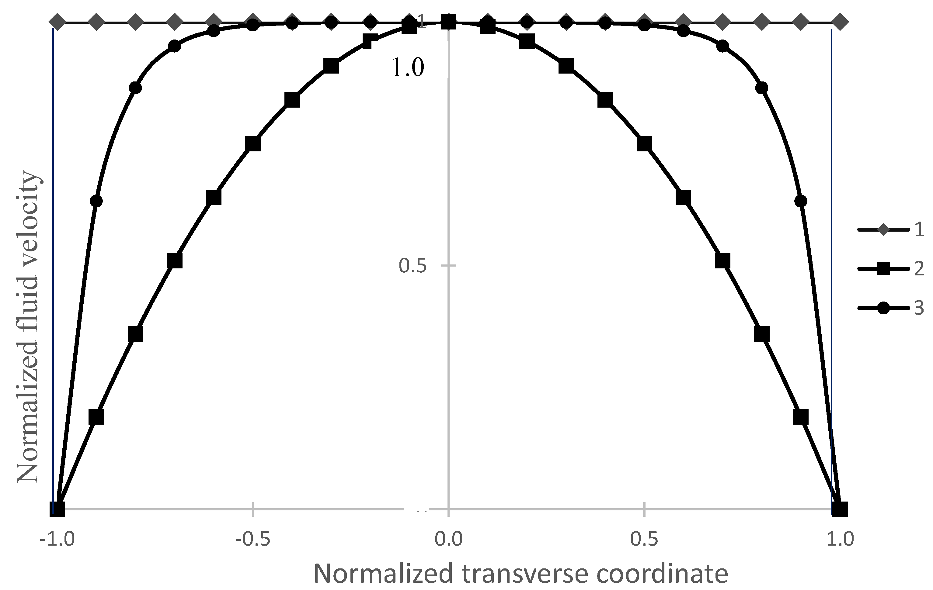
Comparing the solutions corresponding to the Darcy (31), Navier–Stokes (35), and Brinkman models (39) of hydrodynamics, it can be noted that the Darcy model is characterized by a dissipative parameter $K_D$ (Darcy permeability), the Navier–Stokes model is determined by a dissipative parameter $\eta$ (dynamic viscosity), and the Brinkman model is characterized, accordingly, by a combination of two dissipative parameters, $K_D$ and $\eta$.

The velocity profiles shown in Figure 1 are normalized to the value $p_{,x}{K}_D/\eta$, and the transverse coordinate is normalized to the half-width of the capillary $h$.

Darcy model-1, Navier–Stokes model-2 for ${(h/h_m)}^2=h^2/K_D=1$, and Brinkman model-3 for ${(h/h_m)}^2=h^2/K_D=1$.

Let us provide a comparative analysis of the velocity profiles for three models: the Darcy, Navier–Stokes, and Brinkman models. Darcy’s hydrodynamic Equation (30) determines the velocity profile in the capillary that is constant in transverse coordinates, and the Navier–Stokes Equation (34) defines a parabolic velocity profile known as Poiseuille’s law (35). Neither of these two models of hydrodynamics can explain the presence of boundary layers in a liquid, and these two models do not allow one to determine the thickness of these boundary layers that arise near the walls of the capillary. The Brinkman model (38), in contrast to the Darcy and Navier–Stokes models, makes it possible to describe the boundary layer and scale effect associated with the characteristic thickness of the liquid boundary layer $h_m=\sqrt{K_D}$.

Finally, let us analyze the scale effects for the Brinkman model (see Figure 2). It is possible to detect the existence and determine the thickness of the boundary layer only within the framework of Brinkman hydrodynamics (38), when both the first and second dissipation forms (28) and (32) are taken into account in the hydrodynamic equations (see Equation (36)). In the Brinkman model, the motion equations have the form of inhomogeneous Helmholtz equations describing the boundary layer with a characteristic thickness equal to $h_m$. The boundary layer near the walls of the capillary and the corresponding scale effect are taken into account within the framework of the solution obtained above for the Brinkman hydrodynamics model. This is reflected in the structure of the solution (39) and is illustrated by the curves presented in Figure 2, which show the normalized velocity profiles for various values of the dimensionless parameter $h/h_m$.

As a result, in addition to the traditional interpretation of the Darcy parameter $K^D$ as a characteristic of the permeability of the filter medium, another physical interpretation of the permeability coefficient can be proposed as the square of the thickness of the “long” boundary layer characteristic of a given liquid, $K^D=h_m^2$.

6. On Variational Models of Dissipative Heat Transfer Processes

Let us consider irreversible heat transfer processes, the great interest in which is explained by their great applied value. The urgency of the problem of heat transfer and the interest in it are associated with well-known attempts to modify the classical equations of heat conduction to eliminate the contradictions of classical parabolic heat conduction [36,37,38,39] as well as with the desire to modify the theory of heat transfer for modeling size-dependent effects [27,28,40,41,42].

Heat transfer processes are modeled quite well, thanks to the use of first-principles approaches and molecular dynamics methods. On the other hand, methods for experimental evaluation of heat transfer processes are well developed for them. Therefore, it is quite understandable that, recently, there has been a great interest in the study of coupled thermomechanical effects, transients, and scale effects in the problem of heat transfer in homogeneous and inhomogeneous media, including media with a microstructure [27,28,43]. To describe such effects, various modifications of the physical constitutive relations and, accordingly, the heat balance equations are proposed. These modifications are usually introduced phenomenologically to describe specific observed effects. The great importance of variational approaches in relation to such irreversible processes cannot be underestimated; they allow one to obtain energetically consistent mathematical models, regardless of their complexity, which is very important for modeling coupled physical and mechanical effects. In this work, the dissipative component of such processes is proposed to be modeled using the idea of introducing dissipation channels. In the present section we show that the known modifications of the heat conduction laws and the heat balance equations can be constructed by introducing various dissipation channels.

Since heat flux is usually introduced as a temperature gradient, we will proceed to show that it is sufficient to postulate the existence of a scalar potential whose gradient is proportional to temperature to construct a variational model. Indeed, let us postulate the existence of the potential $R$ and introduce the following Lagrangian for the variational problem of a reversible heat transfer process:

$$\begin{array}{l}L=A+K-U, \\ A={\displaystyle \underset{V}{\int }}{P}_{}^{V}RdV+{\displaystyle \underset{F}{\int }}{P}_{}^{F}RdF, K=\frac{1}{2}{\displaystyle \underset{V}{\int }}\tau \dot{R}\dot{R}dV, U=\frac{1}{2}{\displaystyle \underset{V}{\int }}{k}_V{R}_{,k}{R}_{,k}dV\end{array}$$

(40)

Here, $L$ is the dynamic Lagrangian, $A$ is the work of the external forces on the introduced arguments in the volume and on the surface, and $K, U$ are the kinetic and potential energy for the reversible part of the considered processes.

We note that, for brevity—which does not reduce the generality of the proposed approach—we can omit terms appearing outside the volume integral as a result of integration by parts which form the boundary and initial conditions. These terms obviously arise during integration by parts of the variations from the derivatives of arguments. Let us focus exclusively on the equations of constitutive relations and heat transfer equations. We additionally assume, in Equation (40), that $A=0$ and write the following variational equation for considered reversible process:

$$\delta L={\displaystyle \underset{0}{\overset{t}{\int }}}{\displaystyle \underset{V}{\int }}(\tau \dot{R}\delta \dot{R}-k_V{R}_{,i}\delta R_{,i})dVdt={\displaystyle \underset{0}{\overset{t}{\int }}}{\displaystyle \underset{V}{\int }}(k_V\Delta R-\tau \ddot{R})\delta RdVdt+\dots =0$$

(41)

Green’s formulas make it possible to establish constitutive relations for a single scalar force factor and a single vector force factor. These relations can be interpreted as a heat flux and temperature, respectively:

$$T=\partial (K^V-U^V)/\partial \dot{R}=\tau \dot{R}\hspace{1em}{q}_i=\partial (K^V-U^V)/\partial R_{,i}=-k_V{R}_{,i}$$

(42)

where $K^V$ and $U^V$ are the kinetic and potential energy densities, respectively, $2K_V=\tau \dot{R}\dot{R}, 2U_V=k_V{R}_{,k}{R}_{,k}$, and coefficients $k_V$ and $\tau$ allow a physical interpretation as the coefficient of thermal conductivity and the relaxation time for the thermal conductivity flux, respectively, to be applied to them.

Indeed, excluding the scalar potential $R$ in the Euler equation of the variational equality (41) using the constitutive relations (42), we obtain (see also [28,44]):

$$k_V\Delta T-\tau \ddot{T}=0$$

Therefore, the proposed variational model produces, for reversible processes, a heat balance equation of a hyperbolic type (the coefficient $k_V$ is treated as a thermal conductivity coefficient).

To obtain a more complete model of the heat balance equation with the diffusion mechanism of dissipation, we introduce the following dissipation channel, which we will refer to as the Fourier dissipation channel:

$$\overline{\delta U_{1T}}=\frac{1}{2}{\displaystyle \underset{0}{\overset{t}{\int }}}{\displaystyle \underset{V}{\int }}{c}_V(\dot{R}\delta R-R\delta \dot{R})dVdt$$

(43)

We have introduced a coefficient $c_V$ to determine the last dissipation channel (43). In what follows, it will be shown that the coefficient $c_V$ is a physical interpretation of the heat capacity coefficient at constant volume.

Remark 1. 

Note that, in general, we assume that the list of arguments of the dissipative part coincides with the list of arguments of the Lagrange functional for the invertible part. Bilinear terms are sources for formulating dissipative channels. Therefore, for example, the dissipation channel (43) must correspond to a bilinear term $2B R\dot{R}$ in the potential energy density for the reversible part of the functional. Therefore, the full quadratic form in potential energy density must have the form $-A\dot{R}\dot{R}+2B R\dot{R} +CRR$. At the same time, for a specific model, the potential energy density may not contain terms with modules $B$ and/or $C$, because in the reversible part, these modules can be assumed as zero, leaving non-zero corresponding dissipative modules. Hereinafter, we will omit the discussion of the structure for the potential energy and kinetic energy densities, assuming that this question, clearly, can always be solved, whether the variational principle of the problem in the complete formulation is required, including both boundary conditions and “initial” conditions, or not. For example, for dissipation channels containing higher derivatives of generalized variables, reversible processes will correspond to the gradient models, which are easily formulated.

The variational formulation of an irreversible process with a dissipation channel (43) is provided by the following version of Sedov’s variational equality:

$$\begin{array}{l}\delta L-\overline{\delta U_{1T}}={\displaystyle \underset{0}{\overset{t}{\int }}}{\displaystyle \underset{V}{\int }}(\tau \dot{R}\delta \dot{R}-k_V{R}_{,i}\delta R_{,i})dVdt-\frac{1}{2}{\displaystyle \underset{0}{\overset{t}{\int }}}{\displaystyle \underset{V}{\int }}{c}_V(\dot{R}\delta R-R\delta \dot{R})dVdt=\\ ={\displaystyle \underset{0}{\overset{t}{\int }}}{\displaystyle \underset{V}{\int }}[-k_V{R}_{,i}\delta R_{,i}+(c_{V}R+\tau \dot{R})\delta \dot{R}]dVdt+\dots =\\ ={\displaystyle \underset{0}{\overset{t}{\int }}}{\displaystyle \underset{V}{\int }}(k_V\Delta R-\tau \ddot{R}-c_V\dot{R})\delta RdVdt+\dots =0\end{array}$$

(44)

The second line of the equalities (44) provides the structure of constitutive equations

$$\{\begin{array}{l}{q}_i=-k_V{R}_{,i}\\ T=c_{V}R+\tau \dot{R}\hspace{1em}\end{array}$$

(45)

and the last line in (44) is the Euler equation of heat balance, written in terms of the potential $R$:

$$k_V\Delta R-\tau \ddot{R}-c_V\dot{R}=0.$$

Taking into account the second Equation (45), we introduce the temperature operator $T=t(R)$:

$$t(\dots )=c_V(\dots )+\tau {(\dots )}_{,t}$$

(46)

and will use it to eliminate the potential $R$ in physical equations (45) and in the Euler equation.

Indeed, using a temperature operator $t(\dots )$ (46) on the equation of Hooke’s law for the heat flux $q_i$ in (45), we obtain the Maxwell–Cattaneo heat law [27,28,36,37,38,39,45,46,47]:

$$c_V{q}_i+\tau {\dot{q}}_i=-k_V{T}_{,i}$$

(47)

Assume $\tau =0$. Then, we can see that the heat conduction law (47) reduces into the Fourier heat law:

$$c_V{q}_i=-k_V{T}_{,i}$$

Eliminating the potential $R$ with the help of the operator (46) in the Euler Equation (44), we obtain the heat balance equation for the Maxwell-Cattaneo thermal conductivity model, written with respect to temperature [46,47], etc.:

$$k_V\Delta T-\tau \ddot{T}-c_V\dot{T}=0$$

Let us introduce a dissipation channel containing higher order derivatives of generalized variables (see remarks above):

$$\overline{\delta U_{2T}}=\frac{1}{2}{\displaystyle \underset{0}{\overset{t}{\int }}}{\displaystyle \underset{V}{\int }}{a}_2(\Delta R\delta \dot{R}-\dot{R}\delta \Delta R)dVdt$$

(48)

We can assume that the heat conduction equation for the more general process that is being considered is determined as the sum of two dissipation channels, (43) and (48), and the energy density of (40) and (41). Using integration by parts, we write the part of the variational equation that provides the constitutive relations and the Euler equations (heat transfer equation):

$$\begin{array}{l}\delta L-\overline{\delta U_{1T}}-\overline{\delta U_{2T}}=\\ ={\displaystyle \underset{0}{\overset{t}{\int }}}{\displaystyle \underset{V}{\int }}(\tau \dot{R}\delta \dot{R}-k_V{R}_{,i}\delta R_{,i})dVdt-\\ -\frac{1}{2}{\displaystyle \underset{0}{\overset{t}{\int }}}{\displaystyle \underset{V}{\int }}{c}_V(\dot{R}\delta R-R\delta \dot{R})dVdt-\frac{1}{2}{\displaystyle \underset{0}{\overset{t}{\int }}}{\displaystyle \underset{V}{\int }}{a}_2(\Delta R\delta \dot{R}-\dot{R}\delta \Delta R)dVdt+\dots =\\ ={\displaystyle \underset{0}{\overset{t}{\int }}}{\displaystyle \underset{V}{\int }}[(\tau \dot{R}+c_{V}R-a_2\Delta R)\delta \dot{R}-k_V{R}_{,i}\delta R_{,i}]dVdt+\dots =\\ ={\displaystyle \underset{0}{\overset{t}{\int }}}{\displaystyle \underset{V}{\int }}(a_2\Delta \dot{R}+k_V\Delta R-\tau \ddot{R}-c_V\dot{R})\delta RdVdt+\dots =0\end{array}$$

(49)

Constitutive equations of the considered model are provided as follows:

$$\{\begin{array}{l}{q}_i=-k_V{R}_{,i}\\ T=t(R)=c_{V}R+\tau \dot{R}-a_2\Delta R\hspace{1em}\to \hspace{1em}t(\dots )=c_V(\dots )+\tau (\dots {)}_{,t}-a_2\Delta (\dots )\end{array}$$

(50)

and the Euler equation has the following view:

$$(a_2\Delta \dot{R}+k_V\Delta R-\tau \ddot{R}-c_V\dot{R})=0$$

(51)

Using the temperature operator $t(\dots )=c_V(\dots )+\tau {(\dots )}_{,t}-a_2\Delta (\dots )$ on the constitutive relation for the heat flux, (50) we obtain the Guyer–Krumhansl heat conduction law [47]:

$$c_V{q}_i+\tau {\dot{q}}_i-a_2{q}_{j,ji}=-k_V{T}_{,i}$$

(52)

Using the temperature operator $t(\dots )$, (50) for the equation, and (51), we find the heat balance equation corresponding to the Guyer–Krumhansl heat law:

$$a_2\Delta \dot{T}+k_V\Delta T-\tau \ddot{T}-c_V\dot{T}=0$$

(53)

We considered a more complex model whose dissipative properties are determined by a combination of dissipation channels (43), (48), and the following channel:

$$\overline{\delta U_{3T}}=\frac{1}{2}{\displaystyle \underset{V}{\int }}b ({\dot{R}}_{,j}\delta R_{,j}-R_{,j}\delta {\dot{R}}_{,j})dV$$

(54)

The variational model, in this case, is determined by the variational equality:

$$\delta L-\overline{\delta U_{1T}}-\overline{\delta U_{2T}}-\overline{\delta U_{3T}}=0$$

(55)

It is easy to verify that the substitution of the relations (43), (48), (54) in (55), and integration by parts leads, in this case, to the following variational equation:

$$\begin{array}{l}\delta L-\overline{\delta U_{1T}}-\overline{\delta U_{2T}}-\overline{\delta U_{3T}}=\\ ={\displaystyle \underset{V}{\int }}(\tau \dot{R}\delta \dot{R}-k_V{R}_{,i}\delta R_{,i})dV-\frac{1}{2}{\displaystyle \underset{V}{\int }}{c}_V(\dot{R}\delta R-R\delta \dot{R})dV-\\ -\frac{1}{2}{\displaystyle \underset{V}{\int }}a (\Delta R\delta \dot{R}-\dot{R}\delta \Delta R)dV-\frac{1}{2}{\displaystyle \underset{V}{\int }}b ({\dot{R}}_{,j}\delta R_{,j}-R_{,j}\delta {\dot{R}}_{,j})dV+\dots =\\ ={\displaystyle \underset{V}{\int }}[(c_{V}R+\tau \dot{R}-a \Delta R)\delta \dot{R}-(k_V{R}_{,i}+b {\dot{R}}_{,i})\delta R_{,i}]dV=\\ ={\displaystyle \underset{0}{\overset{t}{\int }}}{\displaystyle \underset{V}{\int }}[(a+b)\Delta \dot{R}+k_V\Delta R-\tau \ddot{R}-c_V\dot{R}]\delta RdVdt+\dots =0\end{array}$$

(56)

It follows from constitutive Equation (56) that the considered model can be interpreted as:

$$\{\begin{array}{l}{q}_i=-k_V{R}_{,i}-b {\dot{R}}_{,i}\\ T=t(R)=c_{V}R+\tau \dot{R}-a\Delta R\hspace{1em}\end{array}$$

(57)

The heat transfer equation in terms of the potential R is written as follows (Euler’s equation in (56)):

$$(a+b)\Delta \dot{R}+k_V\Delta R-\tau \ddot{R}-c_V\dot{R}=0$$

(58)

Using the temperature operator $t(R)=c_{V}R+\tau \dot{R}-a \Delta R$ on the first Equation (57), we can exclude the potential R and obtain the Jeffrey-type heat conduction law [43,47]:

$$c_V{q}_i+\tau {\dot{q}}_i-a\Delta q_i=-k_V{T}_{,i}-b {\dot{T}}_{,i}$$

(59)

The last equation for the steady state case has the form:

$$c_V{q}_i-a\Delta q_i=-k_V{T}_{,i}$$

It does not reduce to Fourier’s law for steady state. Notably, the same result was established in [28].

Eliminating the potential R with the help of the constitutive equation for the temperature, i.e., using the temperature operator $t(\dots )$ on (58), we obtain a heat transfer equation with the Jeffrey heat law [48]:

$$(a+b)\Delta \dot{T}+k_V\Delta T-\tau \ddot{T}-c_V\dot{T}=0$$

(60)

Notably, in models (49) and (56), Euler’s equations (the heat transfer Equations (53) and (60)) actually coincide in the terms of the scalar potential $R$; however, the laws of heat conduction and, in general, mathematical formulations are different (compare (52) and (59)).

Obviously, using the technique of introducing dissipation channels, it is possible to establish the variants of high-order theories of heat conduction, not only in relation to material coordinates but also in relation to time. Indeed, we can assume that the dissipative model is constructed as a linear combination of dissipation channels:

$$\overline{\delta U_{1T}}+\overline{\delta U_{2T}}+\overline{\delta U_{3T}}+\overline{\delta U_4}$$

where $\overline{\delta U_4}=\frac{1}{2}{\displaystyle \underset{V}{\int }}c (\ddot{R}\delta \dot{R}-\dot{R}\delta \ddot{R})dV$.

For this case, the generalized thermal conductivity law and heat balance equation can be found as follows:

$$c_V{q}_i+\tau {\dot{q}}_i+c {\ddot{q}}_i-a \Delta q_i=-k_V{T}_{,i}-b {\dot{T}}_{,i}$$

and

$$(a+b)\Delta \dot{T}+k_V\Delta T-c \stackrel{⃛}{T}-\tau \ddot{T}-c_V\dot{T}=0$$

Note that if, in particular, $a+b=0$ in the last equation, then we arrive at an equation of the form:

$$k_V\Delta T-c \stackrel{⃛}{T}-\tau \ddot{T}-c_V\dot{T}=0$$

(61)

In [49], it was shown that heat transfer Equation (61) provides the possibility of predicting, with high precision, that the wave mechanism of heat transfer emerges at low temperatures (ballistic propagation of heat through solids) and of predicting size-dependent effects in thermal conductivity processes.

Remark 2. 

Note that the heat conduction equations require a certain revision concern to the heat flux multiplier: this multiplier must be the specific heat coefficient at a constant volume in order to obtain the correct heat balance equations.

7. Conclusions

We developed a variational principle which makes it possible for the considered model of a reversible process (using a Lagrangian) to add dissipative models by introducing the necessary number of dissipation channels. In particular, examples of formulations of the Darcy, Navier–Stokes, and Brinkman hydrodynamic models were considered. Each of these models is determined by same Lagrangian for the reversible part of process, but with a different set of dissipation channels. In the Brinkman hydrodynamic model, a synergistic effect was discovered which is associated with the simultaneous consideration of the Darcy and Navier–Stokes dissipation channels. This effect explains the existence of a boundary layer in a liquid and the scale effect associated with the thickness of the boundary layer.

Another example of modeling dissipative processes, which may be attractive for applied purposes, is a sequence of variational models of heat transfer processes. All heat conduction laws are obtained as compatibility equations which were received, with the exception of thermal potential, from the equations of Hooke’s law for temperature and heat flow. The laws of thermal conductivity of Fourier, Maxwell–Cattaneo, Guyer–Krumhansl, and Jeffrey are obtained using a proposed universal approach. For different models, different dissipation channels are established, each of which determines the original model of thermal conductivity.