Entanglement and Symmetry Structure of N(= 3) Quantum Oscillators with Disparate Coupling Strengths in a Common Quantum Field Bath

Abstract

In this paper, we study the entanglement structure of a system of N quantum oscillators with distinctive coupling strengths, all linearly coupled to a common massless scalar quantum field. This study is helpful in characterizing the notion of an entanglement domain and its symmetry features, which is useful for understanding the interplay between different levels of structure in many-body quantum systems. The effect of the quantum field on the system is derived via the influence functional and the correlation functions are obtained from the solutions of the evolutionary operator of the reduced density matrix. They are then used to construct the covariance matrix, which forms the basis for our analysis of the structure of quantum entanglement in this open system. To make the physical features explicit, we consider a system of three quantum coupled oscillators placed at the vertices of an equilateral triangle with disparate pairwise couplings. We analyze the entanglement between one oscillator and the other two with equal (symmetric) and unequal (asymmetric) coupling strengths. As a physical illustration, we apply the results for these two different configurations to address some basic issues in macroscopic quantum phenomena from the quantum entanglement perspective.

1. Introduction

Entanglement being an exclusive feature of quantum phenomena [1,2], it is natural to ask how to use entanglement as a clear signifier or distinct marker of the existence of, or, further, a quantitative measure of, the quantum features of many-body quantum systems, and in particular, understanding the theoretical foundation of macroscopic quantum phenomena (MQP) (see, e.g., [3,4,5,6,7,8,9,10,11,12,13,14,15,16,17,18,19,20,21,22,23,24,25,26,27,28,29,30] and references therein). In a series of papers, one of us along with his co-authors have explored three pathways to characterize MQP by way of large N, quantum correlations, and entanglement [31,32,33,34] (see also [35] for further developments). Understanding MQP from an entanglement perspective is an important mission of our research program and the goal of this work.

Regarding the fundamental role that entanglement plays in our understanding of quantum many-body systems, we should mention one very powerful methodology, the tensor network formalism (see, e.g., [36,37,38,39,40,41] and references therein), which has seen great advancement in the last two decades. Here, in contrast, we avoid the complexities and intricacies by staying at a lower structural level and asking just one key question, namely the geometry and symmetry dependence of entanglement. We use a simple model but carry out the analysis of N (here, $N=3$ in detail) coupled harmonic oscillators (see, e.g., [42,43,44] and references therein) with disparate strengths in a common quantum field bath.

In an earlier paper [45], we have studied the distance and coupling dependence of the entanglement between two coupled oscillators in a common quantum field bath. The presence of a quantum field as the environment accords an indirect interaction between the two oscillators at finite separation of a non-Markovian nature [46] that competes with the direct coupling between them (e.g., [47,48,49,50,51]). The interplay between these two factors results in a rich variety of interesting entanglement behaviors. We see from [46] that, at very early times, the indirect non-Markovian interaction between the two oscillators induced by their interaction with the common bath manifests as an interference pattern. But, not too long after that, entanglement is dominated by direct coupling between the two oscillators. Here, we go beyond and work out the entanglement for three oscillators in a common quantum field bath. Not surprisingly, contributions to entanglement under direct coupling between the oscillators dominate over those from the indirect interactions through the bath, with no direct coupling, as was calculated in [52]. With $N=3$, more interesting factors show up: we can see how different coupling strengths change the entanglement structure and how the geometry and symmetry determine the entanglement pattern.

The central issues in MQP that interest us most (see, e.g., [53]) are the identification of the correct levels of structure in a composite body and the judicious choice of the appropriate collective variables, which can capture the essential and different physics of each level. These are often characterized by strong coupling between fine-grained elements or constituents in one particular level of structure (e.g., the level of quarks/gluons or the level of nucleons) and weaker coupling between the elements in a coarser-grained level of structure (e.g., atoms or molecules). Capturing the quantum features of a macroscopic object is greatly facilitated by the existence and functioning of these collective variables depicting a specific level of structure. An exemplary question is: why is it that the Schrodinger equation for the center of mass (CoM) motion of a macroscopic object such as the cantilever in nano-electro and opto-mechanics experiments gives an excellent match with experimental results? Under what conditions can the quantum dynamics of a many-body system be captured well by its CoM? This question was investigated earlier by Chou et al. [54] with a coupled N-oscillator model, where they derived a sufficient condition for this to hold, the so-called “Center of Mass Axiom”.

In Ref. [31] (see also cited work therein, e.g., [55]), the marked difference between entanglement within one specific level of structure and entanglement between different levels of structure is explicated, and how each type would scale with N is identified. These two aspects, namely the role of the CoM in a many-body system and how the level of structure enters in the manifestation of macroscopic quantum phenomena, can be examined by using the entanglement structure results obtained here for a three-oscillator system with disparate coupling strengths.

This paper is organized as follows: in the next section, we derive the late-time covariance matrix elements formed by the canonical variable operators of the N coupled oscillators (for a pedagogical entry into this subject, read, e.g., Section II of [46] for the $N=2$ case). The nonequilibrium evolution of this system under the influence of a quantum scalar field can be derived based on the influence functional formalism approach (for the same purpose, Section II of [45] contains the basics of this methodology). This method first introduced by Feynman and Vernon [56] for the study of quantum Brownian motion has been applied to the derivation of Markovian and non-Markovian master equations for oscillator baths [57,58,59] and for a quantum field environment [60,61]. (For an alternative treatment of an N-oscillator system, see [62] and references therein.) Here, we take the direct route of seeking solutions to the evolutionary operator of the reduced density matrix given formally by Grabert et al. [63] for the derivation of correlation functions. (For an alternative derivation of the non-Markovian master equation and finding their solutions, see [64] and references therein.) In Section 3, the covariance matrix of this system, which is at the heart of our analysis of quantum entanglement, is used to construct the (logarithmic) negativity, a computable and quantifiable quantum measure. In Section 4, we specialize to $N=3$ with disparate coupling and analyze the symmetric and asymmetric configurations described above. In Section 5, we summarize our results and briefly describe their implications for some key issues in MQP and applications in other areas.

2. A System of N Interacting Detectors

We consider a system of N interacting $(i=1$, …, $N)$ detectors where each detector’s internal degree of freedom ${\chi }^{\left(i\right)}\left(t\right)$ is described by a one-dimensional harmonic oscillator. These detectors are allowed to have direct coupling via their internal degrees of freedom, and the coupling term is assumed to be at most quadratic in the internal degrees of freedom. In addition, each oscillator is coupled to a common massless scalar field $\varphi (\mathit{x},t)$ that acts as an environment to the N-oscillator system. As such, there will be indirect interactions between the oscillators mediated by the shared environment. The system with only indirect interaction has been used in [46,52,65,66] to explore the entanglement features.

We consider a system of N detectors, fixed at ${\mathit{z}}^{\left(i\right)}$, and assume that all the oscillators have the same mass m, the same bare frequency ${\omega }_0$, and are acted upon by a harmonic potential of the same form $V\left({\chi }^{\left(i\right)}\right)=m{\omega }_0^2{\chi }^{\left(i\right)}{}^2/2$.

The Lagrangian for the afore-specified system is given by

$$\begin{array}{cc}\hfill S[\chi ,\varphi ]& ={\int }^{t}ds\sum _{i=1}^N\left[\frac{m}{2}{\dot{\chi }}^{\left(i\right)2}\left(s\right)-V\left({\chi }^{\left(i\right)}\right)-\sum _{j>i}^N{V}_{ij}\left(\chi \right)\right]+{\int }^{t}ds\int d^3\mathit{x}\sum _{i=1}^N{j}^{\left(i\right)}(\mathit{x},s)\varphi (\mathit{x},s)\hfill \\ \hfill & +\frac{1}{2}{\int }^{t}ds\int d^3\mathit{x}\left[{\partial }_{\mu }\varphi (\mathit{x},s)\right]\left[{\partial }^{\mu }\varphi (\mathit{x},s)\right],\hfill \end{array}$$

(1)

where $j^{\left(i\right)}(\mathit{x},s)=g_i{\chi }^{\left(i\right)}\left(s\right){\delta }^{\left(3\right)}(\mathit{x}-{\mathit{z}}^{\left(i\right)})$ describes the source that accounts for the interaction between the internal degree of freedom ${\chi }^{\left(i\right)}$ of the $i^{th}$ detector and the environmental scalar field $\varphi$ with coupling strength $g_i$, which we will assume to be weak. The direct coupling between the detectors is given by the interaction potential $V_{ij}$ of the form

$$V_{ij}\left(\chi \right)=\frac{m{\sigma }_{ij}}{2}{\left[{\chi }^{\left(i\right)}\left(s\right)-{\chi }^{\left(j\right)}\left(s\right)\right]}^2,{\sigma }_{ij}={\sigma }_{ji},$$

(2)

with the coupling strength ${\sigma }_{ij}$, which is positive and can be strong. The partial derivative ${\partial }_{\mu }$ in the action of the free scalar field represents ${\partial }_{\mu }=({\partial }_t,\mathsf{\nabla })$, and we choose the Minkowski metric ${\eta }_{\mu \nu }$ with the convention ${\eta }_{\mu \nu }=diag(+,-,-,-)$.

A nice feature of the Gaussian system is that virtually all of the observables can be constructed from the elements of covariance matrix elements due to the Wick expansion [67,68]. In particular, they play a central role in determining the entanglement dynamics of the corresponding system. The covariance matrix $\mathit{V}$ of the N-oscillator system is defined by the expectation values of the anticommutator among the canonical variable operators of the N oscillators

$$\begin{array}{c}\hfill \mathit{V}\left(t\right)=\frac{1}{2}\langle \left\{\mathit{R}\left(t\right),{\mathit{R}}^T\left(t\right)\right\}\rangle ,\end{array}$$

(3)

where $\mathit{R}$ is a column matrix, constituting the canonical variable operators of the N-oscillator system, ${\mathit{R}}^T=({\chi }^{\left(1\right)},p^{\left(1\right)},\dots ,{\chi }^{\left(N\right)},p^{\left(N\right)})$, and $\left\{\mathit{A},\mathit{B}\right\}$ gives the anticommutator of two operators, $\mathit{A}$ and $\mathit{B}$.

Since we are interested only in the late-time entanglement dynamics, the late-time values of the covariance matrix elements will be of our interest, and they are given by, for example,

$$\begin{array}{cc}\hfill \underset{t\to \infty }{lim}\frac{1}{2}\langle \left\{{\chi }^{\left(l\right)}\left(t\right),{\chi }^{\left(m\right)}\left(t\right)\right\}\rangle & =\frac{1}{m}Im{\int }_{-\infty }^{\infty }\frac{d\omega }{2\pi }coth\frac{\beta \omega }{2}{\left[{\tilde{\mathfrak{D}}}_2\left(\omega \right)\right]}_{lm},\hfill \end{array}$$

(4)

$$\begin{array}{cc}\hfill \underset{t\to \infty }{lim}\frac{1}{2}\langle \left\{p^{\left(l\right)}\left(t\right),p^{\left(m\right)}\left(t\right)\right\}\rangle & =mIm{\int }_{-\infty }^{\infty }\frac{d\omega }{2\pi }{\omega }^{2}coth\frac{\beta \omega }{2}{\left[{\tilde{\mathfrak{D}}}_2\left(\omega \right)\right]}_{lm},\hfill \end{array}$$

(5)

and

$$\begin{array}{cc}\hfill \underset{t\to \infty }{lim}\frac{1}{2}\langle \left\{{\chi }^{\left(l\right)}\left(t\right),p^{\left(m\right)}\left(t\right)\right\}\rangle & =0,\hfill \end{array}$$

(6)

where we have chosen $g_i=g$ and defined a new kernel function ${\mathfrak{D}}_2\left(s\right)=\theta \left(s\right){\mathit{D}}_2\left(s\right)$, and its Fourier transform ${\tilde{\mathfrak{D}}}_2\left(\omega \right)$ is given by

$${\tilde{\mathfrak{D}}}_2\left(\omega \right)={\left[-{\omega }^2\mathit{I}+{\Omega }^2-{\displaystyle \frac{g^2}{m}}{\tilde{\mathit{G}}}_R\left(\omega \right)\right]}^{-1},$$

(7)

if we define the Fourier transformation $\tilde{f}\left(\omega \right)$ of a given function $f\left(t\right)$ by

$$\tilde{f}\left(\omega \right)={\int }_{-\infty }^{\infty }d\tau e^{i\omega \tau }f\left(\tau \right).$$

(8)

The matrices ${\mathit{D}}_i$ are a special set of homogeneous solutions

$$\begin{array}{cccccccc}\hfill {\mathit{D}}_1\left(0\right)& ={\mathit{I}}_N,\hfill & \hfill {\dot{\mathit{D}}}_1\left(0\right)& =0,\hfill & \hfill {\mathit{D}}_2\left(0\right)& =0,\hfill & \hfill {\dot{\mathit{D}}}_2\left(0\right)& ={\mathit{I}}_N.\hfill \end{array}$$

to the equation

$$\begin{array}{cc}\hfill m\ddot{\mathit{\chi }}\left(t\right)+m{\Omega }^2·\mathit{\chi }\left(t\right)-{\int }_0^{t}ds{\mathit{G}}_R(t,s)·\mathit{\chi }\left(s\right)& =0,\hfill \end{array}$$

(9)

where the matrix ${\mathit{I}}_N$ is an $N\times N$ identity matrix, and the $N\times N$ interaction matrix ${\Omega }^2$, given by [67]

$${\Omega }^2=\left(\begin{array}{ccccc}{\displaystyle {\omega }_0^2+\sum _{k=1}^N{}^{\prime }{\sigma }_{1k}}& -{\sigma }_{12}& -{\sigma }_{13}& \cdots & -{\sigma }_{1N}\\ -{\sigma }_{21}& {\displaystyle {\omega }_0^2+\sum _{k=1}^N{}^{\prime }{\sigma }_{2k}}& -{\sigma }_{23}& \cdots & -{\sigma }_{2N}\\ -{\sigma }_{31}& -{\sigma }_{32}& \ddots & \cdots & -{\sigma }_{3N}\\ ⋮& ⋮& ⋮& \ddots & ⋮\\ -{\sigma }_{N1}& -{\sigma }_{N2}& -{\sigma }_{N3}& \cdots & {\displaystyle {\omega }_0^2+\sum _{k=1}^N{}^{\prime }{\sigma }_{Nk}}\end{array}\right),$$

(10)

essentially indicates the strength of direct coupling between the internal degrees of freedom of the different detectors. The prime next to the summation, for example,

$${\displaystyle \sum _{k=1}^N{}^{\prime }{\sigma }_{jk},}$$

means that the summation index k runs from 1 to N except for $k=j$.

The matrices ${\mathit{G}}_R(s,s^{\prime })$ in (9), and ${\mathit{G}}_H(s,s^{\prime })$ for the future reference, are of special interest: they are, respectively, the dissipation kernel and the fluctuation kernel [61], defined by

$$\begin{array}{cc}\hfill G_R^{ij}(s,s^{\prime })& =i\theta (s-s^{\prime }){Tr}_{\varphi }\left(\left[\varphi ({\mathit{z}}^{\left(i\right)},s),\varphi ({\mathit{z}}^{\left(j\right)},s^{\prime })\right]\times {\varrho }_{\beta }\right),\hfill \end{array}$$

(11)

$$\begin{array}{cc}\hfill G_H^{ij}(s,s^{\prime })& =\frac{1}{2}{Tr}_{\varphi }\left(\left\{\varphi ({\mathit{z}}^{\left(i\right)},s),\varphi ({\mathit{z}}^{\left(j\right)},s^{\prime })\right\}\times {\varrho }_{\beta }\right),\hfill \end{array}$$

(12)

where $[·,·]$ is the commutator and ${Tr}_{\varphi }$ denotes the trace taken over the field variables. While the noise kernel represents the coarse-grained effect of the environment as stochastic forces, the dissipation kernel captures the damping effect on the detectors’ internal dynamics, in the form of ‘radiation reaction’ or self-force. Ostensibly not to be arbitrarily assigned by hand, they are bound by a set of fluctuation–dissipation relations that should be well known and, in the general case, also a set of propagation–correlation relation that is lesser known [60]. Furthermore, they mediate the response of one detector to the others both by direct couplings amongst the detector and even in the case when there is no direct coupling since the trajectory of each detector affects the field, which in turn affects the other detectors. Therefore, for such an N-detector system, the dynamics are highly non-Markovian. Note, incidentally, that they should not be mistaken as being tensorial quantities: the superscripts i, j are merely labels for the action of the jth detector on the ith detector.

These late-time values (4) and (5) are independent of time and, in particular, Equation (4) has a special significance. It gives the fluctuation–dissipation relations of the reduced system. These relations are connected to the balance of the energy exchange between the N-oscillator system and its surrounding quantum field environment. In turn, this implies the existence of an asymptotic equilibrium state; that is, the N-oscillator system will evolve into an equilibrium state at late times as long as these oscillators are distributed sufficiently locally. A noteworthy feature of the current configuration is that although such a system is coupled to a thermal bath, the final equilibrium state is not necessarily thermal unless the oscillator–bath coupling is vanishingly weak.

The above discussions provide a nice backdrop about the nonequilibrium dynamics of the N-oscillator system under the influences of the environment’s quantum field [56,69,70,71,72,73,74,75,76,77] and facilitate the interpretation of the nonequilibrium evolution of entanglement dynamics.

3. Entanglement and Its Measure

If the joint system can be described by a convex sum of different product states

$$\varrho =\sum _i{p}_i{\varrho }_i^{\left(1\right)}\otimes {\varrho }_i^{\left(2\right)}$$

(13)

where ${\varrho }^{\left(1\right)}$ and ${\varrho }^{\left(2\right)}$ are the density matrices of the respective subsystems, with $p_i>0$ and ${\displaystyle \sum _i{p}_i=1}$, then the corresponding state is called the separable mixed state. From this definition, if a mixed state of a bipartite system cannot be expressed as (13), then the state is entangled.

It has been shown [78,79] that if a mixed state is separable, then the partial transpose of the density matrix remains positive:

$${\varrho }^{p{t}_1}=\sum _i{p}_i{\varrho }_i^{\left(1\right)T}\otimes {\varrho }_i^{\left(2\right)}>0.$$

(14)

where T in the superscript represents the transpose operation. Here, as an example, we perform transposition on only ${\varrho }^{\left(1\right)}$. This is the positive partial transpose (PPT) separability criterion. Thus, in principle, if we find a negative eigenvalue for the partially transposed density matrix, then the corresponding state is entangled. This powerful criterion is further extended to an $M\times N$ bi-partitions of the $(M+N)$-mode bi-symmetric Gaussian system [68,80,81,82,83,84,85,86]. Both sufficient and necessary conditions apply to such a Gaussian system.

When we deal with a system described by continuous variables, the criterion based on the density matrix of the system becomes inconvenient to work with because the dimension of the density matrix for continuous variables is usually infinite. This is where the covariance matrix finds its use. When translated into the covariance matrix, the partial transpose of the density matrix is equivalent to the mirror reflection of the canonical momentum in the corresponding subsystem. Then, a simple, computable, and quantifiable entanglement measure known as logarithmic negativity $E_{\mathcal{N}}$ [85,87,88,89] can be reformulated in terms of the partially transposed covariance matrix. This measure basically collects the symplectic eigenvalues ${\overline{\eta }}_k$ of the partially transposed covariance matrix,

$$E_{\mathcal{N}}=\sum _{k}max\left\{0,-ln2{\overline{\eta }}_k\right\},$$

(15)

and is positive when the state is entangled. In other words, the partially transposed covariance matrix has symplectic eigenvalues ${\overline{\eta }}_k$ smaller than $1/2$ for an entangled state.

4. Disparate Inter-Detector Couplings for N = 3

Now we are in a position to discuss entanglement between three strongly coupled detectors. Let these detectors be labeled by Q, A, and B. Assume that the coupling strength $\lambda$ between the $QA$ pair is the same as that between the $QB$ pair, but different from the coupling strength $\sigma$ between A and B. This leads to an interaction matrix ${\Omega }^2$ of the form

$${\Omega }^2=\left(\begin{array}{ccc}{\omega }_0^2+2\lambda & -\lambda & -\lambda \\ -\lambda & {\omega }_0^2+\lambda +\sigma & -\sigma \\ -\lambda & -\sigma & {\omega }_0^2+\lambda +\sigma \end{array}\right).$$

(16)

It describes the case of disparate coupling between three detectors; that is, ${\sigma }_{12}={\sigma }_{13}=\lambda$ but ${\sigma }_{23}=\sigma$ in (10). These coupling strengths are not assumed weak in comparison with the parameter ${\omega }_0^2$, which is the oscillator frequency of the internal degrees of freedom (or the renormalized oscillating frequency after absorbing the divergence in the retarded Green’s function) in the absence of the inter-detector coupling. Nonetheless, we still assume that the coupling g between the detectors and the environmental scalar field is weak.

4.1. Normal Mode Decomposition

In general, the motion of such a system is highly non-Markovian due to the multi-time correlations generated in the sharing of a common bath [67]. In principle, we would like to decouple their motion by introducing the normal modes, but this is next to impossible for a general non-Markovian system. For certain configurations, this can be achieved. To accomplish this, we first discuss the normal modes, defined with respect to the interaction matrix ${\Omega }^2$. The eigenvalues ${\nu }_i$ and the normalized eigenvectors ${\mathit{v}}_i$ for the interaction matrix ${\Omega }^2$ are given by

$$\begin{array}{cccc}\hfill {\nu }_1& ={\omega }_0^2,\hfill & \hfill {\mathit{v}}_1^T& =\frac{1}{\sqrt{3}}(1,1,1),\hfill \end{array}$$

(17)

$$\begin{array}{cccc}\hfill {\nu }_2& ={\omega }_0^2+3\lambda ,\hfill & \hfill {\mathit{v}}_3^T& =\frac{1}{\sqrt{6}}(2,-1,-1),\hfill \end{array}$$

(18)

$$\begin{array}{cccc}\hfill {\nu }_3& ={\omega }_0^2+\lambda +2\sigma ,\hfill & \hfill {\mathit{v}}_3^T& =\frac{1}{\sqrt{2}}(0,1,-1).\hfill \end{array}$$

(19)

If we construct the matrix $\mathit{U}$ in terms of the normalized eigenvectors, it will transform the interaction matrix ${\Omega }^2$ into the diagonal form ${\Lambda }^2$ by ${\mathit{U}}^T·{\Omega }^2·\mathit{U}$,

$$\mathit{U}=\left(\begin{array}{ccc}{\displaystyle \frac{1}{\sqrt{3}}}& {\displaystyle \frac{2}{\sqrt{6}}}& 0\\ {\displaystyle \frac{1}{\sqrt{3}}}& -{\displaystyle \frac{1}{\sqrt{6}}}& {\displaystyle \frac{1}{\sqrt{2}}}\\ {\displaystyle \frac{1}{\sqrt{3}}}& -{\displaystyle \frac{1}{\sqrt{6}}}& -{\displaystyle \frac{1}{\sqrt{2}}}\end{array}\right),{\Lambda }^2=\left(\begin{array}{ccc}{\omega }_0^2& 0& 0\\ 0& {\omega }_0^2+3\lambda & 0\\ 0& 0& {\omega }_0^2+\lambda +2\sigma \end{array}\right).$$

(20)

Observe that the elements of the ${\Omega }^2$ matrix has the property that

$$\sum _i{\left[{\Omega }^2\right]}_{ij}=\sum _j{\left[{\Omega }^2\right]}_{ij}=\mathrm{const}.,$$

(21)

which is a consequence of the way in which we construct the Lagrangian for inter-detector coupling.

This has a very interesting implication. Suppose that we try to solve the eigenvalue problem for such a system in general. Let the eigenvector $\mathit{v}$ be given by $\mathit{v}={(a_1,a_2,a_3)}^T$; we need to solve a simultaneous set of homogeneous equations

$${\Omega }^2·\mathit{v}=\nu \mathit{v},\Rightarrow \left\{\begin{array}{c}\left({\left[{\Omega }^2\right]}_{11}-\nu \right)a_1+{\left[{\Omega }^2\right]}_{12}{a}_2+{\left[{\Omega }^2\right]}_{13}{a}_3=0,\hfill \\ {\left[{\Omega }^2\right]}_{21}{a}_1+\left({\left[{\Omega }^2\right]}_{22}-\nu \right)a_2+{\left[{\Omega }^2\right]}_{23}{a}_3=0,\hfill \\ {\left[{\Omega }^2\right]}_{31}{a}_1+{\left[{\Omega }^2\right]}_{32}{a}_2+\left({\left[{\Omega }^2\right]}_{33}-\nu \right)a_3=0.\hfill \end{array}\right.$$

(22)

Adding these three equations together leads to

$$\left(\sum _i{\left[{\Omega }^2\right]}_{ij}-\nu \right)\left(a_1+a_2+a_3\right)=0.$$

(23)

Thus, we have either ${\sum }_i{\left[{\Omega }^2\right]}_{ij}-\nu =0$ or $a_1+a_2+a_3=0$. This implies that (i) one of the eigenvalues must be equal to the sum of elements in one of the rows or columns of the matrix ${\Omega }^2$, and that (ii) the elements of the eigenvectors for the rest of the eigenvalues must sum to zero.

From the condition (i), we see from the first equation of (22) that the elements of the corresponding eigenvector must be such that $a_1=a_2=a_3$, so we have

$${\nu }_1=\sum _i{\left[{\Omega }^2\right]}_{i1},{\mathit{v}}_1^T=\frac{1}{\sqrt{3}}(1,1,1),$$

(24)

after proper normalization. The second condition states that the rest of the eigenvector must be normal to the plane $a_1+a_2+a_3=0$. Therefore, as long as the matrix ${\Omega }^2$ satisfies (21), the matrix $\mathit{U}$ that diagonalizes ${\Omega }^2$ will be the same up to the re-ordering of the rows or columns. If we define the normal modes $\mathfrak{v}$ by $\mathfrak{v}={\mathit{U}}^T·r$, then it implies that one of the normal modes, say ${\mathfrak{v}}^{\left(1\right)}$, must be such that

$${\mathfrak{v}}^{\left(1\right)}={\mathit{v}}_1^T·\mathit{r}=\frac{{\mathit{r}}^{\left(1\right)}+{\mathit{r}}^{\left(2\right)}+{\mathit{r}}^{\left(3\right)}}{\sqrt{3}},$$

(25)

which highlights the special role of the center-of-mass coordinate of the original variables of motion. Extension to the case of N detectors is straightforward. This seemingly intuitive yet rarely proven fact will play a key role in our analysis of one important facet of macroscopic quantum phenomena later.

Now, in terms of normal mode variables, the two-point function matrix $\mathit{G}$, shown in (9) for example, will be transformed into

$$\mathfrak{G}={\mathit{U}}^T·\mathit{G}·\mathit{U},$$

(26)

so let us examine the structure of the transformed Green’s function. Generically, we have

$$\begin{array}{cc}\hfill {\mathfrak{G}}^{11}& ={\mathit{G}}^{11}+\frac{2}{3}\left({\mathit{G}}^{12}+{\mathit{G}}^{13}+{\mathit{G}}^{23}\right),\hfill \end{array}$$

(27)

$$\begin{array}{cc}\hfill {\mathfrak{G}}^{12}& =\frac{1}{3\sqrt{2}}\left({\mathit{G}}^{12}+{\mathit{G}}^{13}-2{\mathit{G}}^{23}\right),\hfill \end{array}$$

(28)

$$\begin{array}{cc}\hfill {\mathfrak{G}}^{13}& =\frac{1}{\sqrt{6}}\left({\mathit{G}}^{12}-{\mathit{G}}^{13}\right),\hfill \end{array}$$

(29)

$$\begin{array}{cc}\hfill {\mathfrak{G}}^{23}& =\frac{1}{\sqrt{3}}\left({\mathit{G}}^{12}-{\mathit{G}}^{13}\right),\hfill \end{array}$$

(30)

$$\begin{array}{cc}\hfill {\mathfrak{G}}^{22}& ={\mathit{G}}^{11}+\frac{1}{3}\left(-2{\mathit{G}}^{12}-2{\mathit{G}}^{13}+{\mathit{G}}^{23}\right),\hfill \end{array}$$

(31)

$$\begin{array}{cc}\hfill {\mathfrak{G}}^{33}& ={\mathit{G}}^{11}-{\mathit{G}}^{23}.\hfill \end{array}$$

(32)

due to the fact that ${\mathit{G}}^{11}={\mathit{G}}^{22}={\mathit{G}}^{33}$. If the coupling constant between the oscillator and the environment is the same for all three detectors, and if the distances between any two of the detectors are the same, then we will have ${\mathit{G}}_{ij}$, $i\ne j$ all the same; that is, if the detectors sit at the vertices of an equilateral triangle, the Green function matrix, which describes the backreaction effects from the environment, will take on only two distinct values.

Let ${\mathit{G}}^{11}={\mathit{G}}^{22}={\mathit{G}}^{33}={\mathit{G}}^{\setminus \setminus }$ and ${\mathit{G}}^{ij}={\mathit{G}}^{\times }$ for $i\ne j$. For future reference, we write down the explicit expressions of the retarded Green’s functions, ${\mathit{G}}_R^{\setminus \setminus }$ and ${\mathit{G}}_R^{\times }$,

$$\begin{array}{cccc}\hfill {\mathit{G}}_R^{\setminus \setminus }(\mathit{x},t;,\mathit{x},t^{\prime })& =-\frac{1}{2\pi }\theta \left(\tau \right){\delta }^{\prime }\left(\tau \right),\hfill & \hfill {\mathit{G}}_R^{\times }(\mathit{x},t;{\mathit{x}}^{\prime },t^{\prime })& =\frac{1}{2\pi }\theta (t-t^{\prime })\delta ({\tau }^2-d^2),\hfill \end{array}$$

where $\tau =t-t^{\prime }$ and $d=|\mathit{x}-{\mathit{x}}^{\prime }|$. Furthermore, we immediately see that the consequence of this particular configuration leads to ${\mathfrak{G}}^{ij}=0$ for $i\ne j$, but

$$\begin{array}{cccccc}\hfill {\mathfrak{G}}^{11}& ={\mathit{G}}^{\setminus \setminus }+2{\mathit{G}}^{\times },\hfill & \hfill {\mathfrak{G}}^{22}& ={\mathit{G}}^{\setminus \setminus }-{\mathit{G}}^{\times },\hfill & \hfill {\mathfrak{G}}^{33}& ={\mathit{G}}^{\setminus \setminus }-{\mathit{G}}^{\times }.\hfill \end{array}$$

(33)

In the condensed notation, we will write them as ${\mathit{g}}^{ii}={\mathit{G}}^{\setminus \setminus }+{\alpha }_i{\mathit{G}}^{\times }$, where ${\alpha }_1=2$, ${\alpha }_2={\alpha }_3=-1$. The transformed Green’s function matrix $\mathit{g}$ becomes diagonal, too. This implies that we will have three decoupled equations for the normal modes $\mathfrak{v}$,

$$\begin{array}{cc}\hfill {\ddot{\mathfrak{v}}}_1\left(t\right)+2\gamma {\dot{\mathfrak{v}}}_1\left(t\right)+{\omega }_0^2{\mathfrak{v}}_1\left(t\right)-\frac{4\gamma }{d}{\mathfrak{v}}_1(t-d)& =0,\hfill \end{array}$$

(34)

$$\begin{array}{cc}\hfill {\ddot{\mathfrak{v}}}_2\left(t\right)+2\gamma {\dot{\mathfrak{v}}}_2\left(t\right)+\left({\omega }_0^2+3\lambda \right){\mathfrak{v}}_2\left(t\right)+\frac{2\gamma }{d}{\mathfrak{v}}_2(t-d)& =0,\hfill \end{array}$$

(35)

$$\begin{array}{cc}\hfill {\ddot{\mathfrak{v}}}_3\left(t\right)+2\gamma {\dot{\mathfrak{v}}}_3\left(t\right)+\left({\omega }_0^2+\lambda +2\sigma \right){\mathfrak{v}}_3\left(t\right)+\frac{2\gamma }{d}{\mathfrak{v}}_3(t-d)& =0.\hfill \end{array}$$

(36)

As long as the coupling between the detectors and the environment is sufficiently weak and the distance between detectors is not too short, the time-delay term, which describes the mutual indirect influence between oscillators, only introduces a small correction for the late-time dynamics [46]. Hence, the fundamental solutions to the above equations look like those to the damped oscillators, and are given by

$${\mathfrak{d}}_1^{\left(i\right)}\left(s\right)=e^{-{\Gamma }_{i}s}\left[cos{\Omega }_{i}s+\frac{{\Gamma }_i}{{\Omega }_i}sin{\Omega }_{i}s\right],{\mathfrak{d}}_2^{\left(i\right)}\left(s\right)=e^{-{\Gamma }_{i}s}\frac{1}{{\Omega }_i}sin{\Omega }_{i}s,$$

(37)

where the damping constant ${\Gamma }_i$ and the “resonance” frequency (strictly speaking, this does not look like the resonance frequency. The typical resonance frequency has a contribution of the order ${\gamma }^2$, which is ignored here by the assumption that $1/{\omega }_{i}d\gg \gamma$. However, we should keep in mind that this assumption is not necessary) ${\Omega }_i$ are given by

$${\Gamma }_i=\gamma \left[1+\frac{{\alpha }_i}{{\omega }_{i}d}sin{\omega }_{i}d\right],{\Omega }_i={\omega }_i\left[1-{\alpha }_i\frac{\gamma }{{\omega }_i^{2}d}cos{\omega }_{i}d\right],$$

(38)

in terms of the (renormalized) oscillator frequency ${\omega }_i$

$${\omega }_1^2={\omega }_0^2,{\omega }_2^2={\omega }_0^2+3\lambda ,{\omega }_3^2={\omega }_0^2+\lambda +2\sigma ,$$

(39)

and the parameter $\gamma =g^2/8\pi m$.

4.2. Covariance Matrix of the Normal Modes

Let $\zeta$ denote the normal mode variables of the reduced three-oscillator system $\chi$. Then, it can be shown that the correlations between $\chi$ and their conjugate variables can be expressed in terms of the counterparts of the normal modes $\zeta$; that is,

$$\begin{array}{cccc}\hfill \langle {\chi }_b^{\left(l\right)}{\chi }_b^{\left(m\right)}\rangle & ={\mathit{U}}_{li}{\mathit{U}}_{mj}\langle {\zeta }_b^{\left(i\right)}{\zeta }_b^{\left(j\right)}\rangle ,\hfill & \hfill \langle p_b^{\left(l\right)}{p}_b^{\left(m\right)}\rangle & ={\mathit{U}}_{li}{\mathit{U}}_{mj}\langle {\pi }_b^{\left(i\right)}{\pi }_b^{\left(j\right)}\rangle ,\hfill \end{array}$$

(40)

$$\begin{array}{cc}\hfill \langle {\chi }_b^{\left(l\right)}{p}_b^{\left(m\right)}\rangle & ={\mathit{U}}_{li}{\mathit{U}}_{mj}\langle {\zeta }_b^{\left(i\right)}{\pi }_b^{\left(j\right)}\rangle ,\hfill \end{array}$$

(41)

where ${\pi }^{\left(j\right)}$ is the canonical momentum conjugate to ${\zeta }^{\left(j\right)}$. More importantly, the correlation functions for the normal modes have the same form as those for $\chi$ in (4) and (5) except that all the relevant matrices are replaced by their counterparts associated with the normal modes. This correspondence greatly simplifies the calculation when the normal modes can be completely decoupled, as shown in the configuration introduced previously. Again, these late-time values are also independent of the initial state of the normal mode, such that

$$\begin{array}{cc}\hfill \langle {\zeta }_b^{\left(i\right)2}\rangle & =\frac{1}{m}Im{\int }_{-\infty }^{\infty }\frac{d\omega }{2\pi }{\tilde{\mathfrak{d}}}_2^{\left(i\right)}\left(\omega \right),\hfill \end{array}$$

(42)

$$\begin{array}{cc}\hfill \langle {\pi }_b^{\left(i\right)2}\rangle & =mIm{\int }_{-\infty }^{\infty }\frac{d\omega }{2\pi }{\omega }^2{\tilde{\mathfrak{d}}}_2^{\left(i\right)}\left(\omega \right),\hfill \end{array}$$

(43)

$$\begin{array}{cc}\hfill \langle \{{\zeta }_b^{\left(i\right)},{\pi }_b^{\left(i\right)}\}\rangle & =0,\hfill \end{array}$$

(44)

where ${\tilde{\mathfrak{d}}}_2^{\left(i\right)}$ is the Fourier transformation of the fundamental solution (37) to each normal mode; that is,

$${\tilde{\mathcal{D}}}_2=\left(\begin{array}{ccc}{\tilde{\mathfrak{d}}}_2^{\left(1\right)}& 0& 0\\ 0& {\tilde{\mathfrak{d}}}_2^{\left(2\right)}& 0\\ 0& 0& {\tilde{\mathfrak{d}}}_2^{\left(3\right)}\end{array}\right),$$

(45)

and

$${\tilde{\mathfrak{d}}}_2^{\left(i\right)}\left(\omega \right)={\left[-{\omega }^2+{\omega }_i^2-\frac{g^2}{m}{\tilde{\mathit{g}}}_{ii}\left(\omega \right)\right]}^{-1}={\left[-{\omega }^2+{\omega }_i^2-i2\gamma \omega -2\gamma \frac{{\alpha }_i}{d}{e}^{i\omega d}\right]}^{-1},$$

(46)

and we have used

$${\tilde{\mathit{G}}}^{\setminus \setminus }\left(\omega \right)=\mathrm{div}.+i\frac{\omega }{4\pi },{\tilde{\mathit{G}}}^{\times }\left(\omega \right)=\frac{1}{4\pi d}{e}^{i\omega d}.$$

(47)

The divergence in ${\tilde{\mathit{G}}}^{\setminus \setminus }\left(\omega \right)$ can be absorbed into ${\omega }_i$. Here, we have assumed that we have a zero-temperature bath, so $\beta \to \infty$ and $coth(\beta \omega /2)=1$.

Carrying out the integrals in (42) and (43) gives

$$\begin{array}{cc}\hfill \langle {\zeta }_b^{\left(i\right)2}\rangle & =\frac{1}{2m{\omega }_i}\left\{1-\frac{2}{\pi }\frac{\gamma }{{\omega }_i}+\frac{\gamma {\alpha }_i}{{\omega }_i^{2}d}\left[cos{\omega }_{i}d-\frac{2}{\pi }sin{\omega }_{i}d\right]+\cdots \right\},\hfill \\ \hfill \langle {\pi }_b^{\left(i\right)2}\rangle & =\frac{m{\omega }_i}{2}\left\{1+\frac{2}{\pi }\frac{{\gamma }_i}{\omega }\left(ln\frac{{\Pi }^2}{{\omega }_i^2}-1\right)-\frac{\gamma {\alpha }_i}{{\omega }_i^{2}d}\left[cos{\omega }_{i}d-\frac{2}{\pi }\left(ln\frac{{\Pi }^2}{{\omega }_i^2}-1\right)sin{\omega }_{i}d\right]+\cdots \right\},\hfill \end{array}$$

where $\Pi$ is the cutoff frequency associate with the scalar field, and is assumed to take the same value for all oscillators. Note that the correction due to interaction with the environment is linear in $\gamma$. The damping constant ${\Gamma }_i$ and the resonance frequency ${\Omega }_i$ are given by (38). In the weak coupling limit $\gamma \ll {\omega }_i$, the resonance frequency ${\Omega }_i$ also differs from the normalized oscillating frequency ${\omega }_i$ by the order of $\gamma /{\omega }_i$. Thus, for the leading order, we have

$$\begin{array}{cccc}\hfill \langle {\zeta }_b^{\left(i\right)2}\rangle & \simeq {\displaystyle \frac{1}{2m{\omega }_i}},\hfill & \hfill \langle {\pi }_b^{\left(i\right)2}\rangle & \simeq {\displaystyle \frac{m{\omega }_i}{2}},\hfill \end{array}$$

(48)

as $t\to \infty$.

Next, we can transform the results for the normal modes $\mathbf{\zeta }$ back into the counterparts for the original variables $\mathit{\chi }$ by

$$\begin{array}{cccc}\hfill \langle {\mathit{\chi }}_b^{\phantom{T}}{\mathit{\chi }}_b^T\rangle & =\mathit{U}\langle {\mathbf{\zeta }}_b^{\phantom{T}}{\mathbf{\zeta }}_b^T\rangle {\mathit{U}}^T,\hfill & \hfill \langle {\mathit{p}}_b^{\phantom{T}}{\mathit{p}}_b^T\rangle & =\mathit{U}\langle {\mathbf{\pi }}_b^{\phantom{T}}{\mathbf{\pi }}_b^T\rangle {\mathit{U}}^T.\hfill \end{array}$$

(49)

Explicitly, we have $\langle {\chi }_b^{\left(l\right)}{\chi }_b^{\left(m\right)}\rangle$ given by

$$\begin{array}{cc}\hfill \langle {\chi }_b^{\left(1\right)2}\rangle & =\frac{1}{3}\left[\langle {\zeta }_b^{\left(1\right)2}\rangle +2\langle {\zeta }_b^{\left(2\right)2}\rangle \right],\hfill \end{array}$$

(50)

$$\begin{array}{cc}\hfill \langle {\chi }_b^{\left(2\right)2}\rangle =\langle {\chi }_b^{\left(3\right)2}\rangle & =\frac{1}{6}\left[2\langle {\zeta }_b^{\left(1\right)2}\rangle +\langle {\zeta }_b^{\left(2\right)2}\rangle +3\langle {\zeta }_b^{\left(3\right)2}\rangle \right],\hfill \end{array}$$

(51)

$$\begin{array}{cc}\hfill \langle {\chi }_b^{\left(1\right)}{\chi }_b^{\left(2\right)}\rangle =\langle {\chi }_b^{\left(1\right)}{\chi }_b^{\left(3\right)}\rangle & =\frac{1}{3}\left[\langle {\zeta }_b^{\left(1\right)2}\rangle -\langle {\zeta }_b^{\left(2\right)2}\rangle \right],\hfill \end{array}$$

(52)

$$\begin{array}{cc}\hfill \langle {\chi }_b^{\left(2\right)}{\chi }_b^{\left(3\right)}\rangle & =\frac{1}{6}\left[2\langle {\zeta }_b^{\left(1\right)2}\rangle +\langle {\zeta }_b^{\left(2\right)2}\rangle -3\langle {\zeta }_b^{\left(3\right)2}\rangle \right],\hfill \end{array}$$

(53)

and similar structures for $\langle p_b^{\left(l\right)}{p}_b^{\left(m\right)}\rangle$. Also note that, in these cases, we have $\langle {\chi }_b^{\left(i\right)}{\chi }_b^{\left(j\right)}\rangle =\langle {\chi }_b^{\left(j\right)}{\chi }_b^{\left(i\right)}\rangle$, and thus

$$\frac{1}{2}\langle \{{\chi }_b^{\left(i\right)},{\chi }_b^{\left(j\right)}\}\rangle =\langle {\chi }_b^{\left(i\right)}{\chi }_b^{\left(j\right)}\rangle .$$

(54)

Now it is instructive to make a comparison with the case where there is no inter-detector coupling [52]. In the latter case, the late-time correlation between the variables ${\chi }^{\left(i\right)}$ solely results from their interaction with the environment; thus, it is typically of the order $\gamma$. In addition, as a consequence of the intervention of the background field, this correlation depends on the spatial separation between the detectors. Thus, the detectors tend to have pairwise correlation due to the facts that they have stronger correlation if they get closer to one another, and that additional correlation mediated by the third parties will be at least of the order $\mathcal{O}\left({\gamma }^2\right)$. On the other hand, in the presence of inter-detector coupling, the later-time correlation comes from the superposition of their counterparts from the normal modes; it is of the same order as the uncertainty of the corresponding variables. Thus, the correlation due to inter-detector coupling tends to be much stronger than the induced correlation by the shared bath, and it does not depend on the distance between two detectors. These are the fundamental differences between the two cases studied in the present two papers.

4.3. Bipartite Entanglement

In the subsequent discussion, since the contributions from the environment are much smaller than those from inter-detector coupling, we will only keep terms that are zeroth order in $\gamma$, much like what we carried out in Equation (48). The covariance matrix at the late time is then explicitly given by

$$\mathit{V}=\left(\begin{array}{cccccc}\langle {\chi }_b^{\left(1\right)}{\chi }_b^{\left(1\right)}\rangle & 0& \langle {\chi }_b^{\left(1\right)}{\chi }_b^{\left(2\right)}\rangle & 0& \langle {\chi }_b^{\left(1\right)}{\chi }_b^{\left(3\right)}\rangle & 0\\ 0& \langle p_b^{\left(1\right)}{p}_b^{\left(1\right)}\rangle & 0& \langle p_b^{\left(1\right)}{p}_b^{\left(2\right)}\rangle & 0& \langle p_b^{\left(1\right)}{p}_b^{\left(3\right)}\rangle \\ \langle {\chi }_b^{\left(2\right)}{\chi }_b^{\left(1\right)}\rangle & 0& \langle {\chi }_b^{\left(2\right)}{\chi }_b^{\left(2\right)}\rangle & 0& \langle {\chi }_b^{\left(2\right)}{\chi }_b^{\left(3\right)}\rangle & 0\\ 0& \langle p_b^{\left(2\right)}{p}_b^{\left(1\right)}\rangle & 0& \langle p_b^{\left(2\right)}{p}_b^{\left(2\right)}\rangle & 0& \langle p_b^{\left(2\right)}{p}_b^{\left(3\right)}\rangle \\ \langle {\chi }_b^{\left(3\right)}{\chi }_b^{\left(1\right)}\rangle & 0& \langle {\chi }_b^{\left(3\right)}{\chi }_b^{\left(2\right)}\rangle & 0& \langle {\chi }_b^{\left(3\right)}{\chi }_b^{\left(3\right)}\rangle & 0\\ 0& \langle p_b^{\left(3\right)}{p}_b^{\left(1\right)}\rangle & 0& \langle p_b^{\left(3\right)}{p}_b^{\left(2\right)}\rangle & 0& \langle p_b^{\left(3\right)}{p}_b^{\left(3\right)}\rangle \end{array}\right),$$

(55)

with $\langle {\chi }_b^{\left(i\right)}{\chi }_b^{\left(j\right)}\rangle$ given by (50)–(53) and $\langle {\zeta }_b^{\left(i\right)2}\rangle$, $\langle {\pi }_b^{\left(i\right)2}\rangle$ by (48). Some information of entanglement for this tripartite system can be revealed in the symplectic eigenvalues of a covariance matrix, which correspond to the partially transposed density matrix of this system.

For a system that involves more than two parties, there is more than one way to take the partial transpose of the density matrix. Denote detector 1 as Q, and the remaining two as A and B. We see two distinct cases, one where swapping A and B leads to identical results, because Q is coupled with equal strength $\lambda$ to A and B. This will be what we called the symmetric case, Case [SYM] before. In the other case, which we called Case [ASM] earlier, the entanglement between A and Q is different from that between A and B because the coupling strengths of these pairs are different, being $\lambda$ in the former and $\sigma$ in the latter. Thus, there are two ways to perform the partial transpose. We can either apply it to Q, which will be called Q versus $AB$ (symmetric case). Or, we partially transpose variables associated with A, which will be called A versus $QB$ (asymmetric case).

Recall that the consequence of taking a partial transpose in the density matrix is equivalent to changing the sign of the conjugate momentum of the corresponding subsystem. Take the case Q versus $AB$ for example: the covariance matrix associated with the partial transpose of the subsystem Q becomes

$${\mathit{V}}^{p{t}_Q}=\left(\begin{array}{cccccc}\langle {\chi }_b^{\left(1\right)}{\chi }_b^{\left(1\right)}\rangle & 0& \langle {\chi }_b^{\left(1\right)}{\chi }_b^{\left(2\right)}\rangle & 0& \langle {\chi }_b^{\left(1\right)}{\chi }_b^{\left(3\right)}\rangle & 0\\ 0& \langle p_b^{\left(1\right)}{p}_b^{\left(1\right)}\rangle & 0& -\langle p_b^{\left(1\right)}{p}_b^{\left(2\right)}\rangle & 0& -\langle p_b^{\left(1\right)}{p}_b^{\left(3\right)}\rangle \\ \langle {\chi }_b^{\left(2\right)}{\chi }_b^{\left(1\right)}\rangle & 0& \langle {\chi }_b^{\left(2\right)}{\chi }_b^{\left(2\right)}\rangle & 0& \langle {\chi }_b^{\left(2\right)}{\chi }_b^{\left(3\right)}\rangle & 0\\ 0& -\langle p_b^{\left(2\right)}{p}_b^{\left(1\right)}\rangle & 0& \langle p_b^{\left(2\right)}{p}_b^{\left(2\right)}\rangle & 0& \langle p_b^{\left(2\right)}{p}_b^{\left(3\right)}\rangle \\ \langle {\chi }_b^{\left(3\right)}{\chi }_b^{\left(1\right)}\rangle & 0& \langle {\chi }_b^{\left(3\right)}{\chi }_b^{\left(2\right)}\rangle & 0& \langle {\chi }_b^{\left(3\right)}{\chi }_b^{\left(3\right)}\rangle & 0\\ 0& -\langle p_b^{\left(3\right)}{p}_b^{\left(1\right)}\rangle & 0& \langle p_b^{\left(3\right)}{p}_b^{\left(2\right)}\rangle & 0& \langle p_b^{\left(3\right)}{p}_b^{\left(3\right)}\rangle \end{array}\right),$$

and, likewise for the case A versus $QB$, it is

$${\mathit{V}}^{p{t}_A}=\left(\begin{array}{cccccc}\langle {\chi }_b^{\left(1\right)}{\chi }_b^{\left(1\right)}\rangle & 0& \langle {\chi }_b^{\left(1\right)}{\chi }_b^{\left(2\right)}\rangle & 0& \langle {\chi }_b^{\left(1\right)}{\chi }_b^{\left(3\right)}\rangle & 0\\ 0& \langle p_b^{\left(1\right)}{p}_b^{\left(1\right)}\rangle & 0& -\langle p_b^{\left(1\right)}{p}_b^{\left(2\right)}\rangle & 0& \langle p_b^{\left(1\right)}{p}_b^{\left(3\right)}\rangle \\ \langle {\chi }_b^{\left(2\right)}{\chi }_b^{\left(1\right)}\rangle & 0& \langle {\chi }_b^{\left(2\right)}{\chi }_b^{\left(2\right)}\rangle & 0& \langle {\chi }_b^{\left(2\right)}{\chi }_b^{\left(3\right)}\rangle & 0\\ 0& -\langle p_b^{\left(2\right)}{p}_b^{\left(1\right)}\rangle & 0& \langle p_b^{\left(2\right)}{p}_b^{\left(2\right)}\rangle & 0& -\langle p_b^{\left(2\right)}{p}_b^{\left(3\right)}\rangle \\ \langle {\chi }_b^{\left(3\right)}{\chi }_b^{\left(1\right)}\rangle & 0& \langle {\chi }_b^{\left(3\right)}{\chi }_b^{\left(2\right)}\rangle & 0& \langle {\chi }_b^{\left(3\right)}{\chi }_b^{\left(3\right)}\rangle & 0\\ 0& \langle p_b^{\left(3\right)}{p}_b^{\left(1\right)}\rangle & 0& -\langle p_b^{\left(3\right)}{p}_b^{\left(2\right)}\rangle & 0& \langle p_b^{\left(3\right)}{p}_b^{\left(3\right)}\rangle \end{array}\right).$$

The symplectic eigenvalue $\eta$ of the covariance matrix can be found by solving the eigenvalue problem of the form [90]

$$\mathbf{\sigma }·\mathit{v}=i\eta \mathit{J}·\mathit{v},\mathrm{or}\mathrm{equivalently}i\left(\mathit{J}·\mathbf{\sigma }\right)·\mathit{v}=\eta \mathit{v},$$

(56)

where the matrix $\Sigma$ is the fundamental symplectic matrix

$$\mathit{J}=\underset{k=1}{\overset{N}{⨁}}\left(\begin{array}{cc}0& 1\\ -1& 0\end{array}\right),$$

(57)

and, in our case, $N=3$. The vector $\mathit{v}$ is the corresponding eigenvector. The eigenvalues always appear in pairs and this is most transparent to see in the Williamson normal form of the covariance matrix

$$\underset{k=1}{\overset{n}{⨁}}\left(\begin{array}{cc}{\eta }_k& 0\\ 0& {\eta }_k\end{array}\right),$$

(58)

which is the diagonal form of a symmetric matrix under suitable symplectic transformations. The eigenvalues in our case are then given by the roots to the polynomial

$$det\left({\mathbf{\sigma }}^{pt}-i\eta \mathit{J}\right)=0,$$

(59)

Since it is a third-degree polynomial in ${\eta }^2$, its roots can always be found exactly.

4.4. Entanglement of Q with $AB$

For Q versus $AB$, or what we call the symmetric [SYM] case, the symplectic eigenvalues are

$$\begin{array}{cc}\hfill \eta & =\frac{1}{2},\hfill \\ \hfill {\eta }_{\pm }& ={\left\{\frac{4{\omega }_1^2+{\omega }_1{\omega }_2+4{\omega }_2^2\pm 2\sqrt{2}({\omega }_2-{\omega }_1)\sqrt{(2{\omega }_1+{\omega }_2)({\omega }_1+2{\omega }_2)}}{36{\omega }_1{\omega }_2}\right\}}^{\frac{1}{2}}.\hfill \end{array}$$

They do not depend on ${\omega }_3$, and thus are independent of the coupling constant $\sigma$ between A and B. Among these three eigenvalues, we observe that ${\eta }_{+}$ is always greater than $1/2$, but ${\eta }_{-}$ is always smaller than $1/2$, so it signals the presence of entanglement between Q and the pair $AB$ according to (15). Hence, we only focus on the symplectic eigenvalue ${\eta }_{-}$. In terms of the coupling constant $\lambda$ between Q and A or Q and B, we can show that

$${\eta }_{-}=\left\{\begin{array}{cc}{\displaystyle \frac{1}{2}}-{\displaystyle \frac{\lambda }{2\sqrt{2}{\omega }_0^2}}+\cdots ,\hfill & \lambda \ll {\omega }_0^2,\hfill \\ {\displaystyle \frac{3^{3/4}}{4\sqrt{2}}}{\left({\displaystyle \frac{{\omega }_0^2}{\lambda }}\right)}^{1/4}+\cdots ,\hfill & \lambda \gg {\omega }_0^2,\hfill \end{array}\right.$$

(60)

so it ranges from $1/2$ to 0.

The fact that ${\eta }_{-}$ does not depend on the interaction between A and B may not be that surprising because the interaction between the $QA$ pair is of the same strength as the $QB$ pair; whatever happens between A and B will be “equally” distributed to Q over two channels through the $QA$, $QB$ couplings. This observation is supported by the fact that the correlation functions between the canonical variables associated with Q and A, say $\langle {\chi }_b^{\left(1\right)}{\chi }_b^{\left(2\right)}\rangle$, take on the same value as the corresponding correlation between Q and B, as seen in (52). The value does not depend on the coupling constant between A and B. This balance or symmetry is built-in in the parity between A and B since they start from the same initial configurations, have the same initial oscillating frequency, and are coupled to Q with equal strength. It can be easily disrupted if their motion is out of phase by changing any of the above-mentioned factors or by skewing their relative positions, such that the dependence on $\sigma$ will re-appear.

If we put back the subleading contributions from the influence of the environment, the conclusion that ${\eta }_{-}$ does not depend on $\sigma$ still holds because both A and B experience the same self-force and the same non-Markovian effects mediated by the environment. In comparison, the correlations, say $\langle {\chi }_b^{\left(2\right)}{\chi }_b^{\left(3\right)}\rangle$, between A and B, do depend on the coupling constant $\sigma$ between A and B.

Following this line of reasoning, we see that when the coupling between Q and A (or B) is vanishing small, the entanglement of Q with $AB$ gradually disappears. This is consistent with our intuition because the correlation between Q and A (or B) vanishes, as seen in (52). In this limit, the only connection between Q and A (or B) comes from their coupling to the environment, which is weak. If we even ignore that part, then Q is essentially isolated from A and B. Thus, if Q gets disentangled with $AB$, it will remain disentangled throughout its evolution. On the other hand, if Q interacts strongly with A, their momenta tend to be strongly anti-correlated while their positions remain positively correlated. Meanwhile, the symplectic eigenvalue ${\eta }_{-}$ deviates further away from $1/2$ from below, signaling stronger entanglement between Q and $AB$ in the sense of negativity.

4.5. Entanglement of A with $QB$

Now, turn to the case A versus $QB$. The corresponding symplectic eigenvalues share several identical features as in the case Q versus $AB$. Among the three distinct symplectic eigenvalues, one of them is always greater than $1/2$, the second is equal to $1/2$, and the third one, denoted by ${\eta }_{-}$, is always smaller than $1/2$, regardless of the values of ${\omega }_0^2$, $\lambda$ and $\sigma$:

$$\begin{array}{cc}\hfill \eta & =\frac{1}{2},\hfill \\ \hfill {\eta }_{\pm }& =\frac{1}{72{\omega }_1{\omega }_2{\omega }_3}\left\{2{\omega }_1^2\left(3{\omega }_2+{\omega }_3\right)+2{\omega }_2{\omega }_3\left({\omega }_2+3{\omega }_3\right)+{\omega }_1\left(3{\omega }_2^2-4{\omega }_2{\omega }_3+3{\omega }_3^2\right)\right.\hfill \\ \hfill & \pm \left.\sqrt{-324{\omega }_1^2{\omega }_2^2{\omega }_3^2+{\left[3{\omega }_1{\omega }_2\left(2{\omega }_1+{\omega }_1\right)+2{\left({\omega }_1-{\omega }_2\right)}^2{\omega }_3+3\left({\omega }_1+2{\omega }_2\right){\omega }_3^2\right]}^2}\right\}.\hfill \end{array}$$

Nonetheless, in this case where ${\eta }_{-}$ does depend on the coupling constant $\sigma$ between A and B, generally speaking, for fixed values of ${\omega }_0^2$ and $\lambda$, the symplectic eigenvalue ${\eta }_{-}$ monotonically decreases with larger values of $\sigma$. Therefore, this implies that when the coupling between A and B is stronger than the interaction between Q and A, the entanglement for A versus $QB$ is stronger than the counterpart for Q with $AB$, and vice versa. Thus, the role that inter-detector coupling plays on determining the entanglement structure is more transparent from this comparison. On the other hand, for fixed values of ${\omega }_0^2$ and $\sigma$, the symplectic eigenvalue ${\eta }_{-}$ is not always a monotonically decreasing function of $\lambda$. For small $\lambda$, the value of ${\eta }_{-}$ can increase with $\lambda$ to a maxima and then monotonically decreases. This is particularly significant for larger values of $\sigma$.

To better understand the behavior of ${\eta }_{-}$, let us take a look at some limiting cases: first, suppose that $\lambda$ is vanishingly small and $\sigma$ is fixed in value, and then the only channel for the possible entanglement of A with $QB$ comes from the interaction between A and B. Q is out of reach of A. In this case, we can (wait for the system to reach a steady state and) examine the cross-correlation between them. We see that

$$\begin{array}{cc}\hfill \langle {\chi }_b^{\left(Q\right)}{\chi }_b^{\left(A\right)}\rangle & =\langle {\chi }_b^{\left(Q\right)}{\chi }_b^{\left(B\right)}\rangle =\frac{1}{6m}\left(\frac{1}{{\omega }_1}-\frac{1}{{\omega }_2}\right)=0,\hfill \end{array}$$

(61)

$$\begin{array}{cc}\hfill \langle p_b^{\left(Q\right)}{p}_b^{\left(A\right)}\rangle & =\langle p_b^{\left(Q\right)}{p}_b^{\left(B\right)}\rangle =\frac{m}{6}\left({\omega }_1-{\omega }_2\right)=0,\hfill \end{array}$$

(62)

but

$$\begin{array}{cc}\hfill \langle {\chi }_b^{\left(A\right)}{\chi }_b^{\left(B\right)}\rangle & =\frac{1}{4m}\left(\frac{1}{{\omega }_1}-\frac{1}{{\omega }_3}\right)>0,\hfill \end{array}$$

(63)

$$\begin{array}{cc}\hfill \langle p_b^{\left(A\right)}{p}_b^{\left(B\right)}\rangle & =\frac{m}{4}\left({\omega }_1-{\omega }_3\right)<0,\hfill \end{array}$$

(64)

due to the fact that ${\omega }_3>{\omega }_2={\omega }_1$ in this limit.

Then, we let $\lambda$ increase from zero: there comes an extra channel between A and $QB$ owing to the interaction between A and Q. In addition, B can also be related to A via Q, thus improving the connection between A and $QB$. For $\lambda \ne 0$, we have ${\omega }_3>{\omega }_2>{\omega }_1$ if $\sigma$ is still greater than $\lambda$, so it implies that the cross-correlations then become

$$\begin{array}{cc}\hfill \langle {\chi }_b^{\left(Q\right)}{\chi }_b^{\left(A\right)}\rangle & =\langle {\chi }_b^{\left(Q\right)}{\chi }_b^{\left(B\right)}\rangle =\frac{1}{6m}\left(\frac{1}{{\omega }_1}-\frac{1}{{\omega }_2}\right)>0,\hfill \end{array}$$

(65)

$$\begin{array}{cc}\hfill \langle p_b^{\left(Q\right)}{p}_b^{\left(A\right)}\rangle & =\langle p_b^{\left(Q\right)}{p}_b^{\left(B\right)}\rangle =\frac{m}{6}\left({\omega }_1-{\omega }_2\right)<0,\hfill \end{array}$$

(66)

while

$$\begin{array}{cc}\hfill \langle {\chi }_b^{\left(A\right)}{\chi }_b^{\left(B\right)}\rangle & =\frac{1}{12m}\left[2\left(\frac{1}{{\omega }_1}-\frac{1}{{\omega }_3}\right)+\left(\frac{1}{{\omega }_2}-\frac{1}{{\omega }_3}\right)\right]>0,\hfill \end{array}$$

(67)

$$\begin{array}{cc}\hfill \langle p_b^{\left(A\right)}{p}_b^{\left(B\right)}\rangle & =\frac{m}{12}\left[2\left({\omega }_1-{\omega }_3\right)+\left({\omega }_2-{\omega }_3\right)\right]<0.\hfill \end{array}$$

(68)

As $\lambda$ increases beyond $\sigma$, even when we have ${\omega }_2>{\omega }_3>{\omega }_1$, the cross-correlation between A and B does not change qualitatively. However, we find that both $\langle {\chi }_b^{\left(A\right)}{\chi }_b^{\left(B\right)}\rangle$ and $\langle p_b^{\left(A\right)}{p}_b^{\left(B\right)}\rangle$ reach their extremal values at $\lambda =\sigma$; that is, $\langle {\chi }_b^{\left(A\right)}{\chi }_b^{\left(B\right)}\rangle$ decreases from some positive value as $\lambda$ moves away from zero, until it reaches its minimum at $\lambda =\sigma$. After that point, the correlation between ${\chi }_b^{\left(A\right)}$ and ${\chi }_b^{\left(B\right)}$ monotonically increases with $\lambda$, approaching the value $1/\left(3m{\omega }_1\right)$. The minimum is

$$min\langle {\chi }_b^{\left(A\right)}{\chi }_b^{\left(B\right)}\rangle =\frac{1}{3m}\left(\frac{1}{{\omega }_1}-\frac{1}{{\omega }_2}\right)>0.$$

(69)

On the other hand, the correlation $\langle p_b^{\left(A\right)}{p}_b^{\left(B\right)}\rangle$ increases from some negative values with $\lambda$ until it reaches its maximum value

$$min\langle p_b^{\left(A\right)}{p}_b^{\left(B\right)}\rangle =\frac{m}{3}\left({\omega }_1-{\omega }_2\right)<0,$$

(70)

at $\lambda =\sigma$. Beyond that point, it decreases monotonically without bounds. This partially explains the non-monotonic behavior of ${\eta }_{-}$ for a fixed $\sigma$ because some other factors that enter in determining the covariance matrix, such as $\langle {\chi }_b^{\left(Q\right)}{\chi }_b^{\left(A\right)}\rangle$, do not depend on $\sigma$.

For the case with a fixed $\lambda$, if we let $\sigma =0$—that is, no direct coupling between A and B—the only connection between A and $QB$ results from interaction between A and Q. In this case, B is not entirely out of contact with A. Their correlation can be mediated by Q. Now, we examine their cross-correlation. For $\sigma =0$, we have ${\omega }_2>{\omega }_3>{\omega }_1$, and

$$\begin{array}{cc}\hfill \langle {\chi }_b^{\left(Q\right)}{\chi }_b^{\left(A\right)}\rangle & =\langle {\chi }_b^{\left(Q\right)}{\chi }_b^{\left(B\right)}\rangle =\frac{1}{6m}\left(\frac{1}{{\omega }_1}-\frac{1}{{\omega }_2}\right)>0,\hfill \end{array}$$

(71)

$$\begin{array}{cc}\hfill \langle p_b^{\left(Q\right)}{p}_b^{\left(A\right)}\rangle & =\langle p_b^{\left(Q\right)}{p}_b^{\left(B\right)}\rangle =\frac{m}{6}\left({\omega }_1-{\omega }_2\right)<0.\hfill \end{array}$$

(72)

They are in contrast with (61) and (62). As for the cross-correlation between A and B, we have

$$\begin{array}{cc}\hfill \langle {\chi }_b^{\left(A\right)}{\chi }_b^{\left(B\right)}\rangle & =\frac{1}{12m}\left[2\left(\frac{1}{{\omega }_1}-\frac{1}{{\omega }_3}\right)+\left(\frac{1}{{\omega }_2}-\frac{1}{{\omega }_3}\right)\right]>0,\hfill \end{array}$$

(73)

$$\begin{array}{cc}\hfill \langle p_b^{\left(A\right)}{p}_b^{\left(B\right)}\rangle & =\frac{m}{12}\left[2\left({\omega }_1-{\omega }_3\right)+\left({\omega }_2-{\omega }_3\right)\right]<0.\hfill \end{array}$$

(74)

These qualitative features do not change with increasing $\sigma$. However, there is a major distinction in this case. There is no extremum for the cross-correlation between A and B when we vary $\sigma$. This is consistent with the behavior of ${\eta }_{-}$. Since we have known that the entanglement Q with $AB$ does not depend on $\sigma$, it is equivalent to the special case $\sigma =\lambda$. Therefore, we can draw the conclusion that when the coupling $\sigma$ is greater than $\lambda$, the entanglement for the partition A versus $QB$ is stronger than the counterpart for Q versus $AB$. On the other hand, when the coupling $\sigma$ is weaker than $\lambda$, the entanglement for the partition Q versus $AB$ is stronger than the counterpart for A versus $QB$ (see Figure 1).

Here, we summarize some general features of cross-correlations. It has been shown that with stronger inter-oscillator couplings, the cross-correlation $\langle {\chi }^{\left(i\right)}{\chi }^{\left(j\right)}\rangle$ tends to be more strongly correlated, with the exception that $\langle {\chi }^{\left(Q\right)}{\chi }^{\left(A\right)}\rangle$ is not sensitive to the coupling strength $\sigma$ between A and B. On the other hand, $\langle p^{\left(i\right)}{p}^{\left(j\right)}\rangle$ tends to be more strongly anti-correlated with stronger inter-oscillator couplings. We also observe that since $\langle {\chi }^{\left(i\right)}{\chi }^{\left(j\right)}\rangle$ is bounded, they do not change appreciably with $\lambda$ and $\sigma$. In contrast, $\langle p^{\left(i\right)}{p}^{\left(j\right)}\rangle$ is not bounded below; it can vary more dramatically with the coupling constants $\lambda$ and $\sigma$. In particular, $\langle p^{\left(A\right)}{p}^{\left(B\right)}\rangle$ varies more significantly with $\sigma$ but less with $\lambda$, while $\langle p^{\left(Q\right)}{p}^{\left(A\right)}\rangle$ changes more notably with $\lambda$ but is independent of $\sigma$.

In conclusion, we see from this detailed analysis how the entanglement structure of coupled quantum oscillators depends on the coupling strength, from knowledge of the cross-correlations between the oscillators. This quantitative description is valuable in aiding our understanding of entanglement behavior because it is the simplest continuous variable many-body system that is amenable to such a detailed analysis. For larger systems with more components and less symmetry, this becomes dauntingly challenging. We shall explore the implications of our results for some key issues in macroscopic quantum phenomena in the next section.

5. Summary of Results and Implications

The effects of field-induced interaction on quantum entanglement between two harmonic oscillators have been studied earlier, notably in [45,46,65,66,91,92,93,94]. One interesting feature shown there is the distance dependence of quantum entanglement, since the coupling is mediated by a quantum field whose influence varies with time and space. In [52], a model of N quantum oscillators located at different fixed positions in space, which do not interact with each other directly but only through weak couplings to a common scalar massless quantum field, was studied. After coarse-graining the quantum field, a late-time covariance matrix of this open system of N oscillators with only indirect field-induced coupling was derived and analyzed. For $N=3$, it was found that, in the weak coupling limit, the correlations adopt a simple pairwise structure, in that the correlation between any two oscillators is ignorant of the presence of the other oscillator. The way in which one oscillator’s presence alters the entanglement of the other two was used in [52] to capture a novel notion called an ‘entanglement domain’. This paper studies the entanglement structure of the N quantum oscillator system sharing a common quantum scalar field environment but, unlike these two earlier papers, we allow the oscillators to have direct pairwise couplings of disparate strengths.

5.1. Comparison with Case without Direct Coupling

The salient features based on detailed studies of the $N=3$ case, as we have seen, turn out to be quite different from the case of N oscillators with only field-induced coupling. The first entanglement feature, namely that the correlation between any two oscillators is ignorant of the presence of the other oscillator, is no longer true. The second feature, namely the distance dependence of entanglement due to each oscillator’s coupling to a quantum field, is now no longer prominent, being overwhelmed by the direct couplings. We see that each case studied in these two papers captures one aspect of the overall behavior of the system of N oscillators: while the first case may depict neutral atoms, the latter case depicts ions (in an open quantum field rather than in a cavity or in a trap). The idealized model study here, though not a replica of actual experimental setups, can nonetheless provide us with a clear theoretical understanding and quantitative description of the entanglement structure of such commonly encountered continuous-variable quantum systems.

5.2. Summary of Direct Disparate Coupling Results

• Entanglement for the N-oscillator system with direct coupling is decided by whether any of the symplectic eigenvalues of the partially transposed covariance matrix are smaller than $1/2$.
• Entanglement is enhanced by stronger coupling between any two oscillators, as in intuitive reasoning.
• Two cases of different symmetries are studied in detail here, where three oscillators are placed at the vertices of an equilateral triangle. Call one of the oscillators Q, which is distinguished from the other two, A and B, by different couplings. Consider the two cases: Case [SYM], where Q is equally coupled to A and B (symmetric configuration), versus Case [ASY], where A is coupled to Q differently from its coupling to B (asymmetric configuration). The main features are:

Symmetric versus asymmetric cases

• CASE [SYM] Q vs. $AB$, where Q is coupled to A and B with equal strength: the entanglement of Q with $AB$ as a group is independent of the coupling between A and B. It is as if Q is entangled with a ‘center-of-mass’ variable of the two oscillators $AB$ as a group.
• CASE [ASY] A vs. $QB$, where the coupling strength between A and Q is different from that between A and B: entanglement for A vs. $QB$ does depend on $QA$ coupling and $AB$ coupling.

  (a)

  For a fixed $QA$ coupling, the entanglement measure is a monotonically decreasing function of $AB$ coupling; the symplectic eigenvalue ${\eta }_{-}$ of the partially transposed covariance matrix in this case ranges from $1/2$ to 0. (Further deviation from $1/2$ means increasing entanglement.)

  (b)

  For a fixed $AB$ coupling, the entanglement measure does not always monotonically decrease with increasing $QA$ coupling. It increases first to reach the maximum and then monotonically decreases. This is due to the effect of cross-correlations.

  (c)

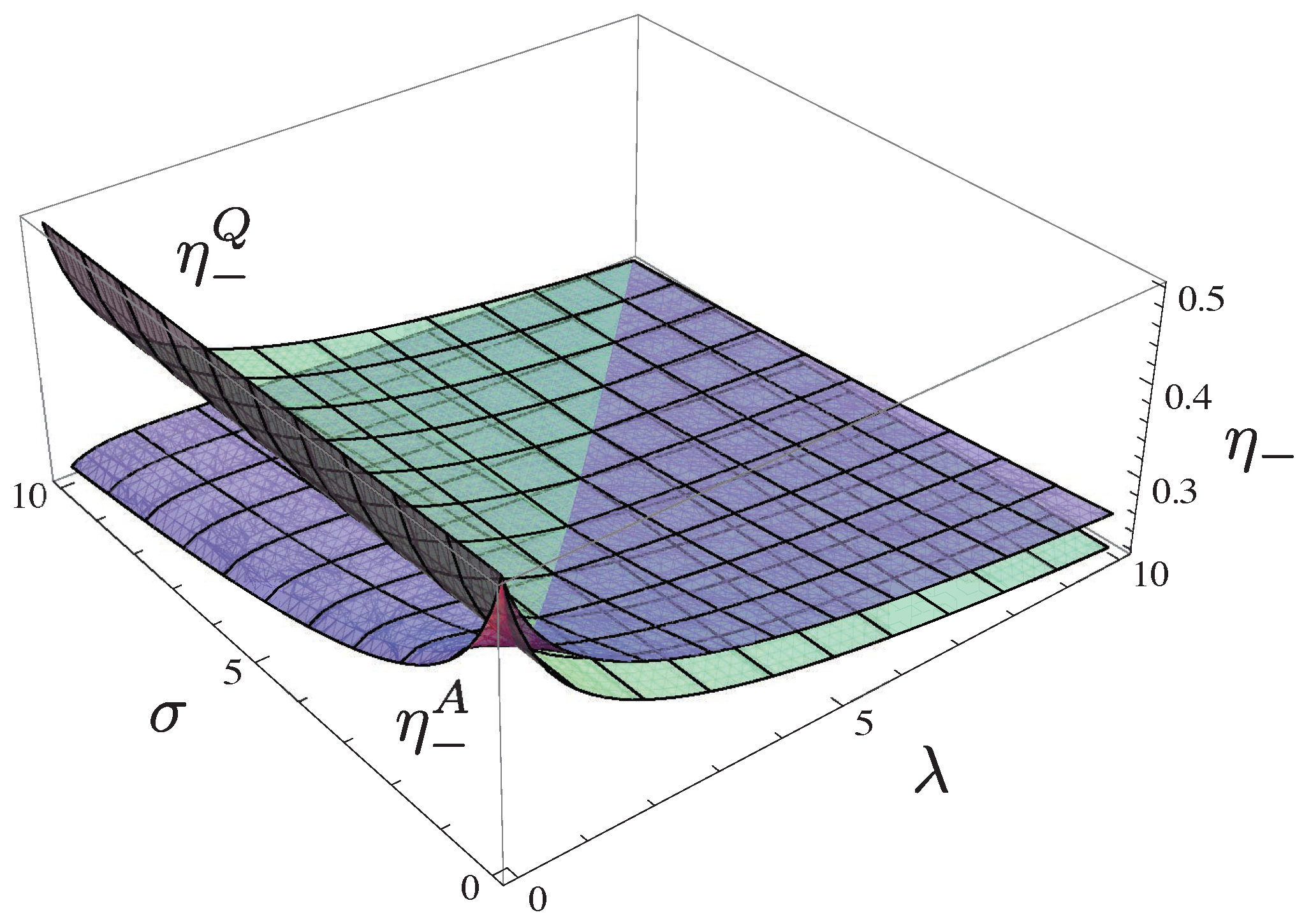
  For $QA$ and $QB$ coupling greater than $AB$ coupling, entanglement for Q vs. $AB$ is stronger than entanglement A vs. $QB$.

  (d)

  For $AB$ coupling greater than $QA$ coupling, entanglement for A vs. $QB$ is stronger than that for Q vs. $AB$

5.3. Implications for Issues in Meso- and Macroscopic Quantum Phenomena

As mentioned in the introduction, one emergent area of research that results from this analysis can be applied to is macroscopic quantum phenomena. We identified two key issues to explore: one is the role of the CoM in the quantum behavior of a many-body system and the other is how the level of structure manifests in macroscopic quantum phenomena. They can be examined using the entanglement structure results obtained here for a three-oscillator system with disparate coupling strengths.

In the SYM case, we show that, as far as quantum entanglement is concerned, Q is effectively coupled to the CoM of A and B. This shows that, for quantum behavior of this nature, the CoM variable plays a role similar to that in classical mechanics. Now, view Q as the center of mass variable representing a macroscopic object 1, and A, B as representative constituents of a similar macroscopic object 2. One interesting result of of relevance to the level-of-structure aspect of MQP that we found here is that (at least for quadratic inter-particle coupling) the entanglement between Q and $AB$ is equivalent to that between Q and the CoM of 2, independent of the coupling between A and B, provided that A and B are interchangeably identically. This is of interest because it explains why as one reports on the quantum dynamics of, say, a cantilever (e.g., [18,21]), one does not need to also provide information on how the nucleons in the metal bar are coupled. A comparison of the results between the [SYM] and the [ASY] cases is also informative about why levels of structure, or a hierarchical ordering in the organization of matter [29], facilitates a better understanding of the manifestation of quantum behavior of macroscopic objects.

The open system of an N coupled quantum oscillator system is a generic model for investigating continuous-variable quantum many-body systems under different environmental influence. Toward understanding macroscopic quantum phenomena from the entanglement perspective, an important contributing factor is the identical particle or indistinguishability issue, such as that discussed in, e.g., [95,96,97,98,99]. In addition to the entanglement aspects explored here, the ‘size or large N’ and the ‘correlation or infrared behavior’ aspects of MQP for interacting quantum systems as explained in [32,33,34] are also of interest. We can mention two easily extrapolated directions. One is to assume the presence of finite temperature fields whereby one can investigate issues in quantum thermodynamics such as those related to thermal entanglement [42,43,100,101], which underlie MQP in biological systems. One can also partition the N oscillators into two parts: one consisting of m oscillators representing the system and the second part consisting of $n=N-m$ oscillators as the bath. By varying m versus n or varying the inter- and intra-coupling strengths, one can investigate new facets of mesoscopic phenomena [81,102,103,104]. Doing so in a microscopic model enables one to monitor or even control the emergence of macroscopic quantum phenomena, possibly showing up in different patterns.

References

- Schrödinger, E. Discussion of probability relations between separated systems. Math. Proc. Camb. Phil. Soc. 1935, 31, 553. [Google Scholar] [CrossRef]
- Schrödinger, E. Probability relations between separated systems. Math. Proc. Camb. Phil. Soc. 1936, 32, 446. [Google Scholar] [CrossRef]
- Leggett, A.J. Macroscopic quantum systems and the quantum theory of measurement. Prog. Theo. Phys. Supp. 1980, 69, 80. [Google Scholar] [CrossRef]
- Ghirardi, G.C.; Rimini, A.; Weber, T. Unified dynamics for microscopic and macroscopic systems. Phys. Rev. D 1986, 34, 470. [Google Scholar] [CrossRef]
- Pearle, P. Combining stochastic dynamical state-vector reduction with spontaneous localization. Phys. Rev. A 1989, 39, 2277. [Google Scholar] [CrossRef]
- Ghirardi, G.C.; Pearle, P.; Rimini, A. Markov processes in Hilbert space and continuous spontaneous localization of systems of identical particles. Phys. Rev. A 1990, 42, 78. [Google Scholar] [CrossRef]
- Bassi, A.; Ghirardi, G.C. Dynamical reduction models. Phys. Rep. 2003, 379, 257. [Google Scholar] [CrossRef]
- Diosi, L. Gravitation and quantum-mechanical localization of macro-objects. Phys. Lett. A 1984, 105, 199. [Google Scholar] [CrossRef]
- Diosi, L. A universal master equation for the gravitational violation of quantum mechanics. Phys. Lett. A 1987, 120, 377. [Google Scholar] [CrossRef]
- Diosi, L. Models for universal reduction of macroscopic quantum fluctuations. Phys. Rev. A 1989, 40, 1165. [Google Scholar] [CrossRef]
- Károlyházy, F.; Frenkel, A.; Lukács, B. Quantum Concepts in Space and Time; Penrose, R., Isham, C.J., Eds.; Oxford University Press: Oxford, UK, 1986. [Google Scholar]
- Penrose, R. On gravity’s role in quantum state reduction. Gen. Relativ. Gravit. 1986, 28, 581–600. [Google Scholar] [CrossRef]
- Penrose, R. Quantum computation, entanglement and state reduction. Phil. Trans. R. Soc. A 1998, 356, 1927. [Google Scholar] [CrossRef]
- Bardeen, J. Superconductivity and other macroscopic quantum phenomena. Phys. Today 1990, 43, 25. [Google Scholar] [CrossRef]
- Arndt, M.; Nairz, O.; Vos-Andreae, J.; Keller, C.; Van der Zouw, G.G.; Zeilinger, A. Wave–particle duality of C60 molecules. Nature 1999, 401, 680. [Google Scholar] [CrossRef] [PubMed]
- Leggett, A.J. Testing the limits of quantum mechanics: Motivation, state of play, prospects. J. Phys. Condens. Matter 2002, 14, R415. [Google Scholar] [CrossRef]
- Takagi, S. Macroscopic Quantum Tunneling; Cambridge University Press: Cambridge, UK, 2005; Available online: https://www.cambridge.org/us/universitypress/subjects/physics/condensed-matter-physics-nanoscience-and-mesoscopic-physics/macroscopic-quantum-tunneling (accessed on 1 November 2023).
- Armour, A.; Blencowe, M.; Schwab, K. Entanglement and decoherence of a micromechanical resonator via coupling to a Cooper-pair box. Phys. Rev. Lett. 2002, 88, 148301. [Google Scholar] [CrossRef] [PubMed]
- Marshall, W.; Simon, C.; Penrose, R.; Bouwmeester, D. Towards quantum superpositions of a mirror. Phys. Rev. Lett. 2003, 91, 130401. [Google Scholar] [CrossRef]
- Müller-Ebhardt, H.; Rehbein, H.; Schnabel, R.; Danzmann, K.; Chen, Y. Entanglement of macroscopic test masses and the standard quantum limit in laser interferometry. Phys. Rev. Lett. 2008, 100, 013601. [Google Scholar] [CrossRef]
- Gröblacher, S.; Hammerer, K.; Vanner, M.R.; Aspelmeyer, M. Observation of strong coupling between a micromechanical resonator and an optical cavity field. Nature 2009, 460, 724. [Google Scholar] [CrossRef]
- Marquardt, F.; Girvin, S.M. Optomechanics. Physics 2009, 2, 40. [Google Scholar] [CrossRef]
- Meystre, P. A short walk through quantum optomechanics. Ann. Phys. 2012, 525, 215. [Google Scholar] [CrossRef]
- Bassi, A.; Lochan, K.; Satin, S.; Singh, T.P.; Ulbricht, H. Models of wave-function collapse, underlying theories, and experimental tests. Rev. Mod. Phys. 2012, 85, 471. [Google Scholar] [CrossRef]
- Chen, Y. Macroscopic quantum mechanics: Theory and experimental concepts of optomechanics. J. Phys. B 2013, 46, 104001. [Google Scholar] [CrossRef]
- Aspelmeyer, M.; Kippenberg, T.J.; Marquardt, F. Cavity optomechanics. Rev. Mod. Phys. 2014, 86, 1391. [Google Scholar] [CrossRef]
- Gröblacher, S.; Trubarov, A.; Prigge, N.; Cole, G.D.; Aspelmeyer, M.; Eisert, J. Observation of non-Markovian micromechanical Brownian motion. Nat. Comm. 2015, 6, 7606. [Google Scholar] [CrossRef]
- Anastopoulos, C.; Lagouvardos, M.; Savvidou, K. Gravitational effects in macroscopic quantum systems: A first-principles analysis. Class. Quan. Grav. 2021, 38, 155012. [Google Scholar] [CrossRef]
- Hu, B.L. Quantum hierarchical systems: Fluctuation force by coarse-graining, decoherence by correlation noise. In From Quantum to Classical: Essays in Memory of Dieter Zeh; Kiefer, C., Ed.; Springer: Cham, Switzerland, 2022. [Google Scholar] [CrossRef]
- Kaltenbaek, R.; Arndt, M.; Aspelmeyer, M.; Barker, P.F.; Bassi, A.; Bateman, J.; Belenchia, A.; Bergé, J.; Braxmaier, C.; Bose, S.; et al. Research campaign: Macroscopic quantum resonators (MAQRO). Quant. Sci. Technol. 2023, 8, 014006. [Google Scholar] [CrossRef]
- Hu, B.L.; Subaşı, Y. Pathways toward understanding Macroscopic Quantum Phenomena. J. Phys. Conf. Ser. 2013, 442, 012010. [Google Scholar] [CrossRef]
- Chou, C.-H.; Hu, B.L.; Subaşı, Y. Macroscopic quantum phenomena from the large N perspective. J. Phys. Conf. Ser. 2011, 306, 012002. [Google Scholar] [CrossRef]
- Chou, C.-H.; Hu, B.L.; Subaşı, Y. Macroscopic quantum phenomena from the correlation, coupling and criticality perspectives. J. Phys. Conf. Ser. 2011, 330, 012003. [Google Scholar] [CrossRef]
- Chou, C.-H.; Subasi, Y.; Hu, B.L. Macroscopic quantum phenomena from the coupling pattern and entanglement structure perspective. arXiv 2013. [Google Scholar] [CrossRef]
- Kao, J.-Y.; Chou, C.-H. Quantum entanglement in coupled harmonic oscillator systems: From micro to macro. New J. Phys. 2016, 18, 073001. [Google Scholar] [CrossRef]
- Evenbly, G.; Vidal, G. Tensor network states and geometry. J. Stat. Phys. 2011, 145, 891. [Google Scholar] [CrossRef]
- Orús, R. A practical introduction to tensor networks: Matrix product states and projected entangled pair states. Ann. Phys. 2014, 349, 117. [Google Scholar] [CrossRef]
- Orús, R. Tensor networks for complex quantum systems. Nat. Rev. Phys. 2019, 1, 538. [Google Scholar] [CrossRef]
- Strathearn, A. Modelling Non-Markovian Quantum Systems Using Tensor Networks; Springer: Cham, Switzerland, 2020. [Google Scholar] [CrossRef]
- Colafranceschi, E.; Oriti, D. Quantum gravity states, entanglement graphs and second-quantized tensor networks. J. High Energy Phys. 2021, 2021, 1. [Google Scholar] [CrossRef]
- Tao, X. Density Matrix and Tensor Network Renormalization; Cambridge University Press: Cambridge, UK, 2023; Available online: https://www.cambridge.org/tw/universitypress/subjects/physics/condensed-matter-physics-nanoscience-and-mesoscopic-physics/density-matrix-and-tensor-network-renormalization?format=HB (accessed on 1 November 2023).
- Audenaert, K.; Eisert, J.; Plenio, M.B.; Werner, R.F. Entanglement properties of the harmonic chain. Phys. Rev. A 2002, 66, 042327. [Google Scholar] [CrossRef]
- Amico, L.; Fazio, R.; Osterloh, A.; Vedral, V. Entanglement in many-body systems. Rev. Mod. Phys. 2008, 80, 517. [Google Scholar] [CrossRef]
- de Ponte, M.A.; Mizrahi, S.S.; Moussa, M.H.Y. Networks of dissipative quantum harmonic oscillators: A general treatment. Phys. Rev. A 2007, 76, 032101. [Google Scholar] [CrossRef]
- Hsiang, J.-T.; Hu, B.L. Distance and coupling dependence of entanglement in the presence of a quantum field. Phys. Rev. D 2015, 92, 125026. [Google Scholar] [CrossRef]
- Lin, S.-Y.; Hu, B.L. Temporal and spatial dependence of quantum entanglement from a field theory perspective. Phys. Rev. D 2009, 79, 085020. [Google Scholar] [CrossRef]
- Duarte, O.S.; Caldeira, A.O. Effective coupling between two Brownian particles. Phys. Rev. Lett. 2006, 97, 250601. [Google Scholar] [CrossRef]
- Chou, C.-H.; Yu, T.; Hu, B.L. Exact master equation and quantum decoherence of two coupled harmonic oscillators in a general environment. Phys. Rev. E 2008, 77, 011112. [Google Scholar] [CrossRef] [PubMed]
- Paz, J.P.; Roncaglia, A.J. Dynamics of the entanglement between two oscillators in the same environment. Phys. Rev. Lett. 2008, 100, 220401. [Google Scholar] [CrossRef] [PubMed]
- Duarte, O.S.; Caldeira, A.O. Effective quantum dynamics of two Brownian particles. Phys. Rev. A 2009, 80, 032110. [Google Scholar] [CrossRef]
- Cacheffo, A.; Moussa, M.H.Y.; de Ponte, M.A. The double Caldeira–Leggett model: Derivation and solutions of the master equations, reservoir-induced interactions and decoherence. Phys. A 2010, 389, 2198. [Google Scholar] [CrossRef]
- Zhou, R.; Hu, B.L. Entanglement structure of an open system of N quantum oscillators, I: Field-induced coupling N=3. arXiv 2013, arXiv:1306.3728. [Google Scholar]
- Hu, B.L. Emergent/quantum gravity: Macro/micro structures of spacetime. J. Phys. Conf. Ser. 2009, 174, 012015. [Google Scholar] [CrossRef]
- Chou, C.-H.; Hu, B.L.; Yu, T. Quantum Brownian motion of a macroscopic object in a general environment. Phys. A 2008, 387, 432. [Google Scholar] [CrossRef]
- Martins, A.M. Macroscopic entanglement between wave-packets at finite temperature. arXiv 2012. [Google Scholar] [CrossRef]
- Feynman, R.P.; Vernon, F. The theory of a general quantum system interacting with a linear dissipative system. Ann. Phys. 1963, 24, 118. [Google Scholar] [CrossRef]
- Caldeira, A.O.; Leggett, A.J. Path integral approach to quantum Brownian motion. Phys. A 1983, 121, 587. [Google Scholar] [CrossRef]
- Hu, B.L.; Paz, J.P.; Zhang, Y. Quantum Brownian motion in a general environment: Exact master equation with nonlocal dissipation and colored noise. Phys. Rev D 1992, 45, 2843. [Google Scholar] [CrossRef] [PubMed]
- Hu, B.L.; Matacz, A. Quantum Brownian motion in a bath of parametric oscillators: A model for system-field interactions. Phys. Rev. D 1994, 49, 6612. [Google Scholar] [CrossRef]
- Raval, A.; Hu, B.L.; Anglin, J. Near-thermal radiation in detectors, mirrors, and black holes: A stochastic approach. Phys. Rev. D 1996, 53, 7003. [Google Scholar] [CrossRef]
- Johnson, P.R.; Hu, B.L. Stochastic theory of relativistic particles moving in a quantum field: Scalar Abraham-Lorentz-Dirac-Langevin equation, radiation reaction, and vacuum fluctuations. Phys. Rev. D 2002, 65, 065015. [Google Scholar] [CrossRef]
- Fleming, C.H.; Roura, A.; Hu, B.L. Quantum Brownian motion of multipartite systems and their entanglement dynamics. arXiv 2011. [Google Scholar] [CrossRef]
- Grabert, H.; Schramm, P.; Ingold, G.L. Quantum Brownian motion: The functional integral approach. Phys. Rep. 1988, 168, 115. [Google Scholar] [CrossRef]
- Calzetta, E.; Roura, A.; Verdaguer, E. Stochastic description for open quantum systems. Phys. A 2003, 319, 188. [Google Scholar] [CrossRef]
- Lin, S.-Y.; Chou, C.-H.; Hu, B.L. Disentanglement of two harmonic oscillators in relativistic motion. Phys. Rev. D 2008, 78, 125025. [Google Scholar] [CrossRef]
- Lin, S.-Y.; Hu, B.L. Entanglement creation between two causally disconnected objects. Phys. Rev. D 2010, 81, 045019. [Google Scholar] [CrossRef]
- Hsiang, J.-T.; Chou, C.-H.; Subaşı, Y.; Hu, B.L. Quantum thermodynamics from the nonequilibrium dynamics of open systems: Energy, heat capacity, and the third law. Phys. Rev. E 2018, 97, 012135. [Google Scholar] [CrossRef] [PubMed]
- Simon, R. Peres-Horodecki separability criterion for continuous variable systems. Phys. Rev. Lett. 2000, 84, 2726. [Google Scholar] [CrossRef]
- Schwinger, J.S. Brownian motion of a quantum oscillator. J. Math. Phys. 1961, 2, 407. [Google Scholar] [CrossRef]
- Keldysh, L. Diagram technique for nonequilibrium processes. Zh. Eksp. Teor. Fiz. 1964, 47, 1515. Available online: http://jetp.ras.ru/cgi-bin/dn/e_020_04_1018.pdf (accessed on 1 November 2023).
- Chou, K.-C.; Su, Z.-B.; Hao, B.-L.; Yu, L. Equilibrium and non-equilibrium formalisms made unified. Phys. Rep. 1985, 118, 1. [Google Scholar] [CrossRef]
- Weiss, U. Quantum Dissipative Systems, 4th ed.; World Scientific: Singapore, 2012. [Google Scholar] [CrossRef]
- Breuer, H.P.; Petruccione, F. The Theory of Open Quantum Systems, 2nd ed.; Oxford University Press: Oxford, UK, 2007. [Google Scholar] [CrossRef]
- Rivas, A.; Huelga, S.F. Open Quantum Systems: An Introduction; Springer: Berlin/Heidelberg, Germany, 2012. [Google Scholar] [CrossRef]
- Calzetta, E.; Hu, B.L. Nonequilibrium Quantum Field Theory; Cambridge University Press: Cambridge, UK, 2008. [Google Scholar] [CrossRef]
- Kamenev, A. Field Theory of Non-Equilibrium Systems; Cambridge University Press: Cambridge, UK, 2011. [Google Scholar] [CrossRef]
- Rammer, J. Quantum Field Theory of Non-Equilibrium States; Cambridge University Press: Cambridge, UK, 2009. [Google Scholar] [CrossRef]
- Peres, A. Separability criterion for density matrices. Phys. Rev. Lett. 1996, 77, 1413. [Google Scholar] [CrossRef]
- Horodecki, M.; Horodecki, P.; Horodecki, R. Separability of mixed states: Necessary and sufficient conditions. Phys. Lett. A 1996, 223, 1. [Google Scholar] [CrossRef]
- Simon, R.; Mukunda, N.; Dutta, B. Quantum-noise matrix for multimode systems: U(n) invariance, squeezing, and normal forms. Phys. Rev. A 1994, 49, 1567. [Google Scholar] [CrossRef]
- Serafini, A.; Adesso, G.; Illuminati, F. Unitarily localizable entanglement of Gaussian states. Phys. Rev. A 2005, 71, 032349. [Google Scholar] [CrossRef]
- Adesso, G.; Serafini, A.; Illuminati, F. Quantification and scaling of multipartite entanglement in continuous variable systems. Phys. Rev. Lett. 2004, 93, 220504. [Google Scholar] [CrossRef] [PubMed]
- Adesso, G.; Illuminati, F. Gaussian measures of entanglement versus negativities: Ordering of two-mode Gaussian states. Phys. Rev. A 2005, 72, 032334. [Google Scholar] [CrossRef]
- Serafini, A.; Illuminati, F.; De Siena, S. Symplectic invariants, entropic measures and correlations of Gaussian states. J. Phys. B 2004, 37, L21. [Google Scholar] [CrossRef]
- Adesso, G.; Illuminati, F. Entanglement in continuous-variable systems: Recent advances and current perspectives. J. Phys. A 2007, 40, 7821. [Google Scholar] [CrossRef]
- Adesso, G. Entanglement of Gaussian States. Ph.D. Thesis, University of Salerno, Salerno, Italy, 2006. [Google Scholar] [CrossRef]
- Vidal, G.; Werner, R.F. Computable measure of entanglement. Phys. Rev. A 2002, 65, 032314. [Google Scholar] [CrossRef]
- Plenio, M.B. The logarithmic negativity: A full entanglement monotone that is not convex. Phys. Rev. Lett. 2005, 65, 95. [Google Scholar] [CrossRef]
- Werner, R.F.; Wolf, M.M. Bound entangled Gaussian states. Phys. Rev. Lett. 2001, 86, 3658. [Google Scholar] [CrossRef]
- Williamson, J. On the algebraic problem concerning the normal forms of linear dynamical systems. Am. J. Math. 1936, 58, 141. [Google Scholar] [CrossRef]
- Hsiang, J.-T.; Hu, B.L. ‘Hot entanglement’?—A nonequilibrium quantum field theory scrutiny. Phy. Lett. B 2015, 750, 396. [Google Scholar] [CrossRef]
- Hsiang, J.-T.; Hu, B.L. Quantum entanglement at high temperatures? bosonic systems in nonequilibrium steady state. J. High Energy Phys. 2015, 2015, 90. [Google Scholar] [CrossRef]
- Hsiang, J.-T.; Arısoy, O.; Hu, B.L. Entanglement dynamics of coupled quantum oscillators in independent nonMarkovian baths. Entropy 2022, 24, 1814. [Google Scholar] [CrossRef] [PubMed]
- Arısoy, O.; Hsiang, J.-T.; Hu, B.L. Hot entanglement?—Parametrically coupled quantum oscillators in two heat baths: Instability, squeezing and driving. J. High Energy Phys. 2023, 2023, 122. [Google Scholar] [CrossRef]
- Horodecki, M.; Sen, A.; Sen, U.; Horodecki, K. Local indistinguishability: More nonlocality with less entanglement. Phys. Rev. Lett. 2003, 90, 047902. [Google Scholar] [CrossRef] [PubMed]
- Killoran, N.; Cramer, M.; Plenio, M.B. Extracting entanglement from identical particles. Phys. Rev. Lett. 2014, 112, 150501. [Google Scholar] [CrossRef] [PubMed]
- Bose, S.; Home, D. Duality in entanglement enabling a test of quantum indistinguishability unaffected by interactions. Phys. Rev. Lett. 2013, 110, 140404. [Google Scholar] [CrossRef] [PubMed]
- Brünner, T.; Dufour, G.; Rodríguez, A.; Buchleitner, A. Signatures of indistinguishability in bosonic many-body dynamics. Phys. Rev. Lett. 2018, 120, 210401. [Google Scholar] [CrossRef]
- Benatti, F.; Floreanini, R.; Franchini, F.; Marzolino, U. Entanglement in indistinguishable particle systems. Phys. Rep. 2020, 878, 1. [Google Scholar] [CrossRef]
- Anders, J.; Winter, A. Entanglement and separability of quantum harmonic oscillator systems at finite temperature. Quan. Inf. Comput. 2008, 8, 245. [Google Scholar] [CrossRef]
- Anders, J. Thermal state entanglement in harmonic lattices. Phys. Rev. A 2008, 77, 062102. [Google Scholar] [CrossRef]
- Plyukhin, A.V.; Schofield, J. Stochastic dynamics with a mesoscopic bath. Phy. Rev. E 2001, 64, 041103. [Google Scholar] [CrossRef]
- Hasegawa, H. Classical small systems coupled to finite baths. Phy. Rev. E 2011, 83, 021104. [Google Scholar] [CrossRef]
- Hasegawa, H. Specific heat anomalies of small quantum systems subjected to finite baths. J. Math. Phys. 2011, 52, 123301. [Google Scholar] [CrossRef]
Disclaimer/Publisher’s Note: The statements, opinions and data contained in all publications are solely those of the individual author(s) and contributor(s) and not of MDPI and/or the editor(s). MDPI and/or the editor(s) disclaim responsibility for any injury to people or property resulting from any ideas, methods, instructions or products referred to in the content. |
© 2023 by the authors. Licensee MDPI, Basel, Switzerland. This article is an open access article distributed under the terms and conditions of the Creative Commons Attribution (CC BY) license (https://creativecommons.org/licenses/by/4.0/).
Share and Cite
Hsiang, J.-T.; Hu, B.-L. Entanglement and Symmetry Structure of N(= 3) Quantum Oscillators with Disparate Coupling Strengths in a Common Quantum Field Bath. Symmetry 2023, 15, 2064. https://doi.org/10.3390/sym15112064
Hsiang J-T, Hu B-L. Entanglement and Symmetry Structure of N(= 3) Quantum Oscillators with Disparate Coupling Strengths in a Common Quantum Field Bath. Symmetry. 2023; 15(11):2064. https://doi.org/10.3390/sym15112064
Chicago/Turabian StyleHsiang, Jen-Tsung, and Bei-Lok Hu. 2023. "Entanglement and Symmetry Structure of N(= 3) Quantum Oscillators with Disparate Coupling Strengths in a Common Quantum Field Bath" Symmetry 15, no. 11: 2064. https://doi.org/10.3390/sym15112064