

Solutions of Magnetohydrodynamics Equation through Symmetries
 , , and
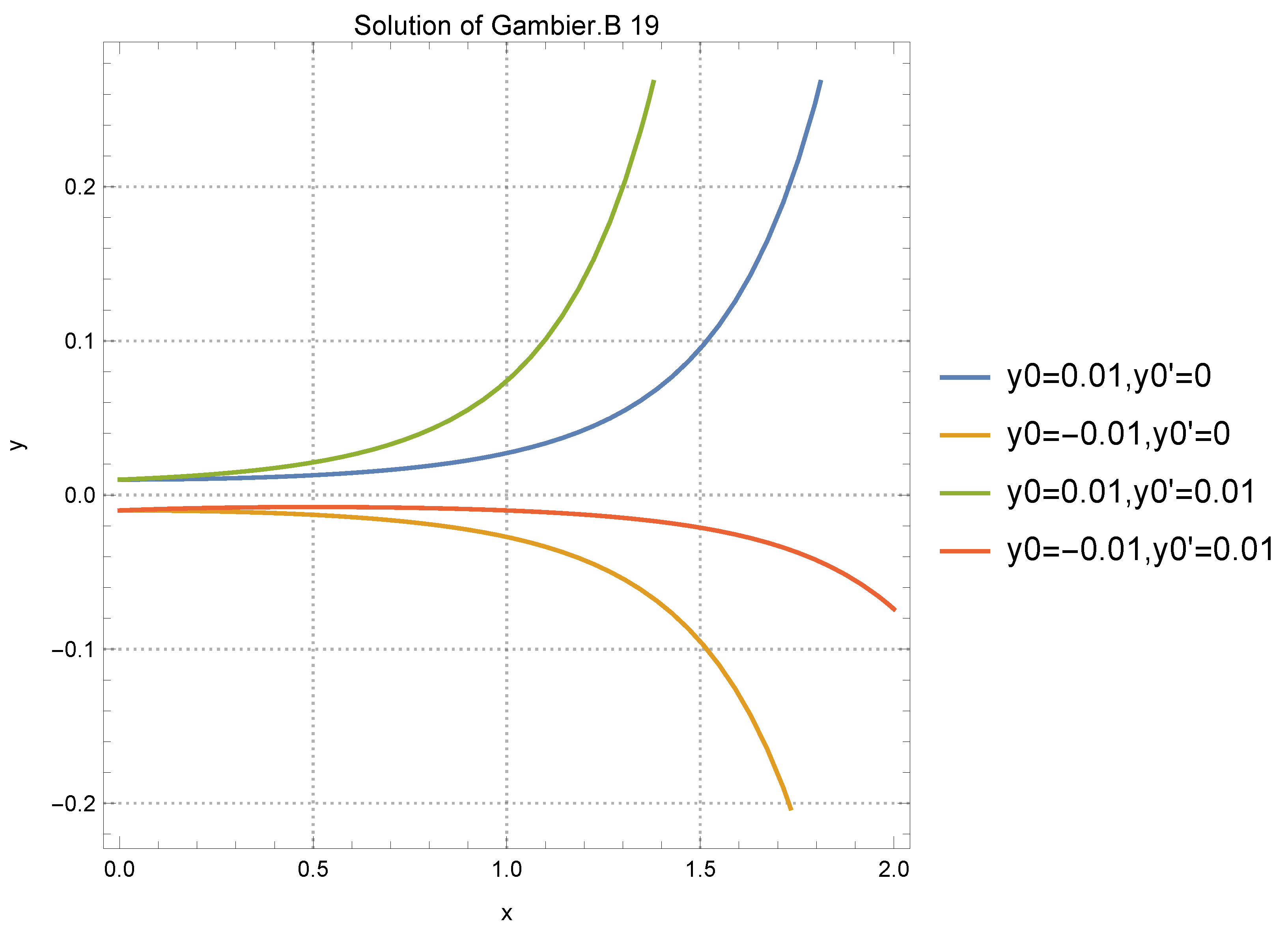
Abstract
:1. Introduction
2. Preliminaries
3. Lie Symmetries of the Magnetohydrodynamics Equation
4. Reduction to an Ordinary Differential Equation
5. Particular Cases of Equation (28)
5.1. Case 1 (Gambier.B 19)
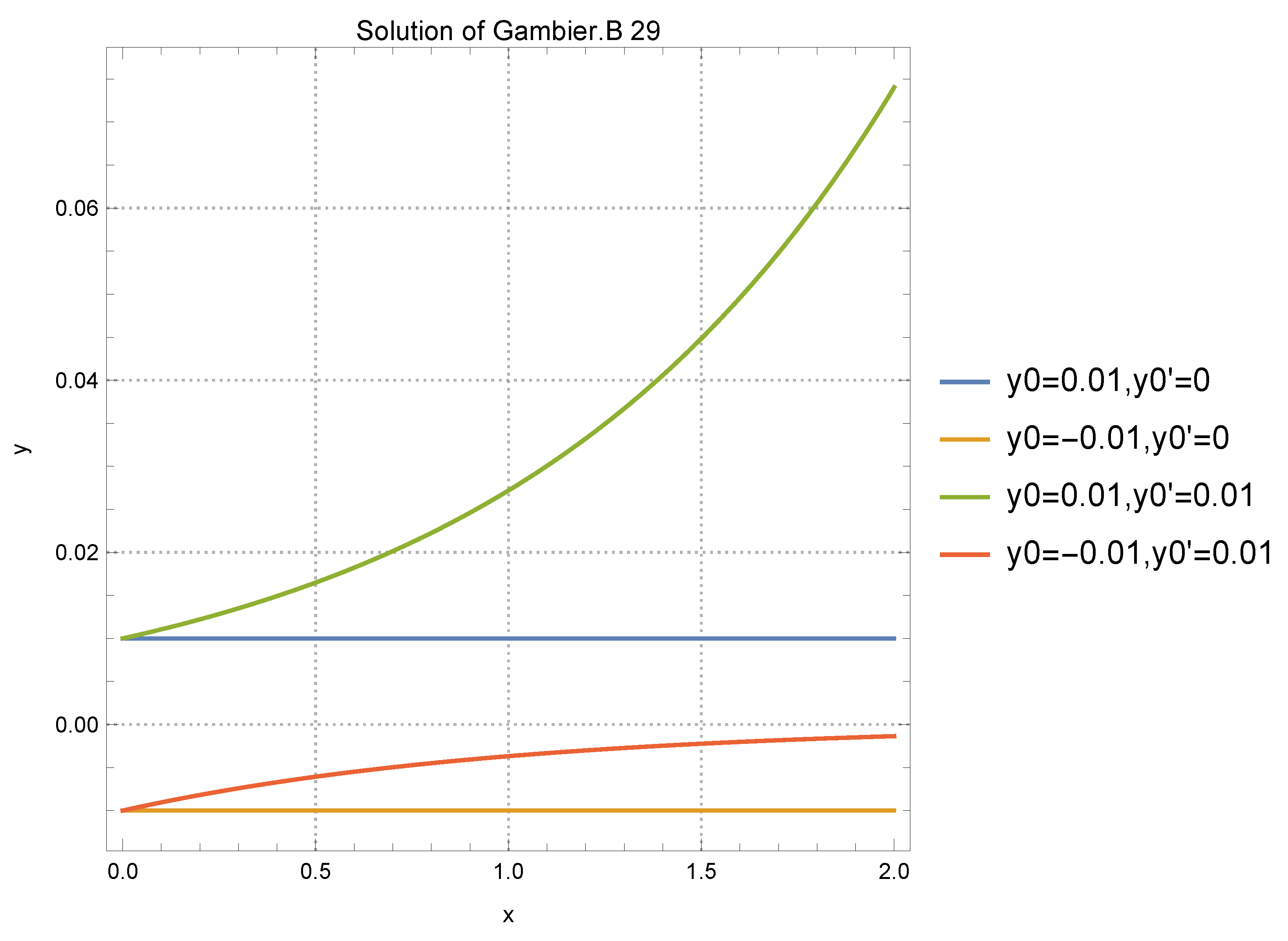
5.2. Case 2 (Gambier.B 29)
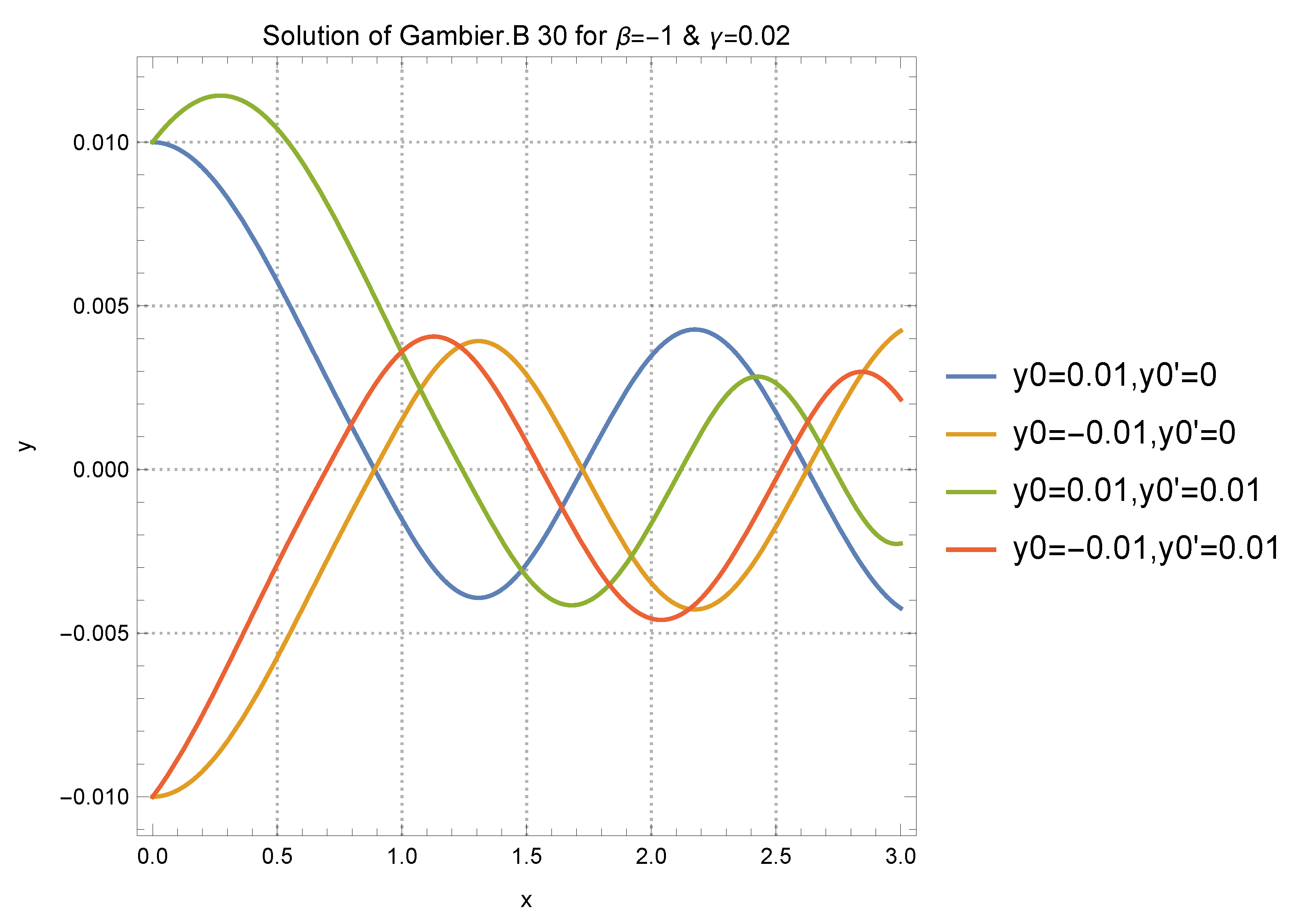
5.3. Case 3 (Gambier.B 30)
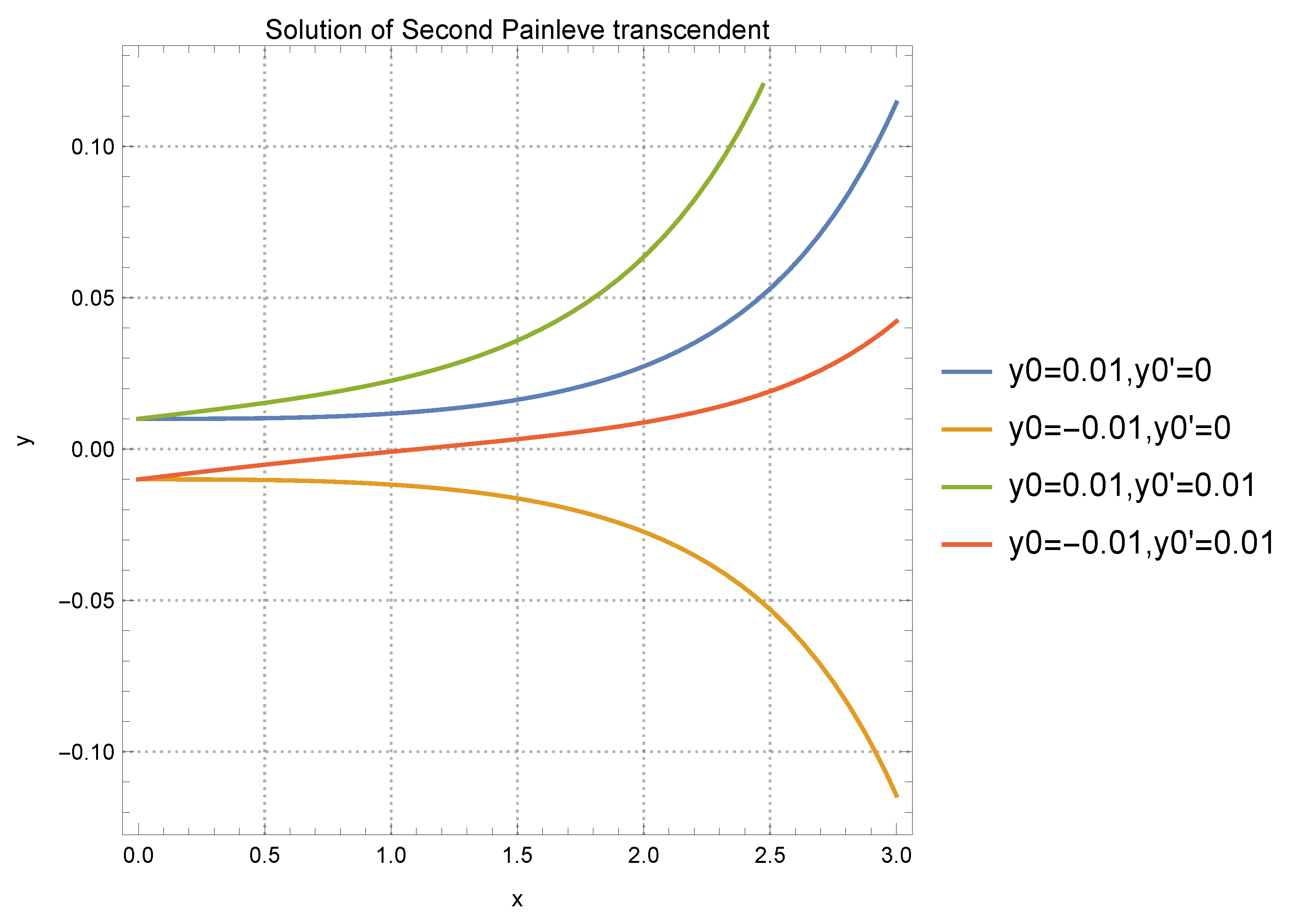
5.4. Case 4 (Second Painlevé Transcendent)
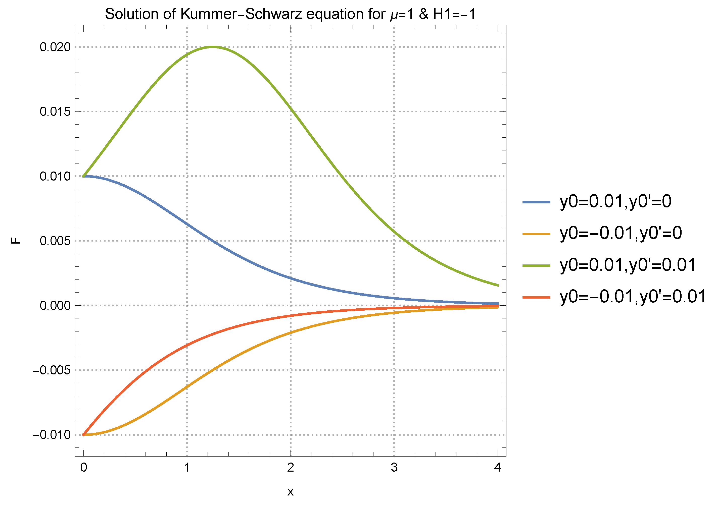
5.5. Case 5 (Kummer–Schwarz Equation)
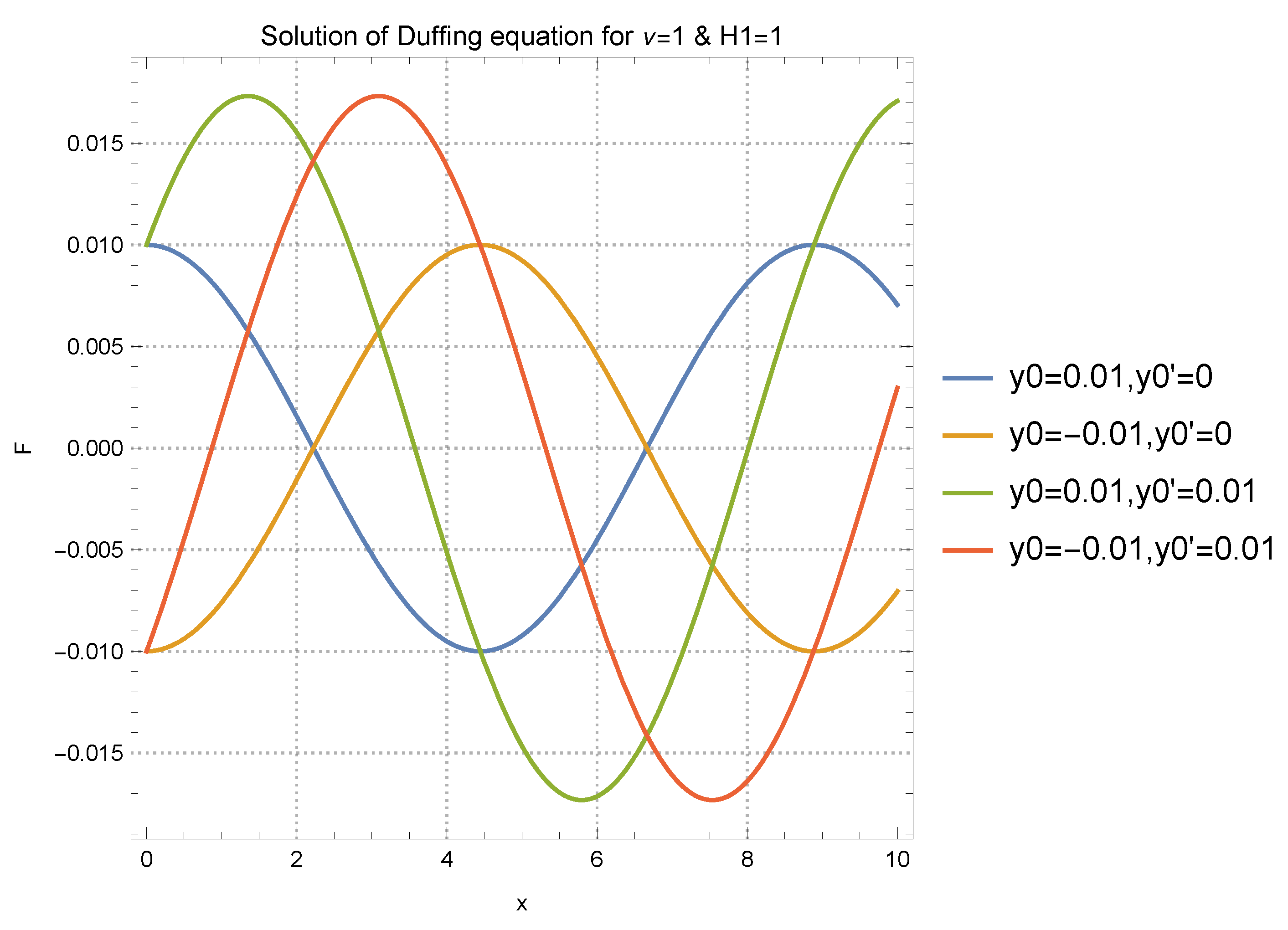
5.6. Case 6 (Duffing Equation)
6. General Cases of Equation (29)
6.1. Case 7 Gambier.B 28
6.2. Case 8 Gambier.B 27
7. The Case f = 0, g = 0
7.1. Case 6a
7.2. Case 6b
8. Conclusions
Author Contributions
Funding
Data Availability Statement
Conflicts of Interest
References
- Fleischer, J.; Diamond, P.H. Compressible Alfven turbulence in one dimension. Phys. Rev. E 1998, 58, R2709. [Google Scholar] [CrossRef]
- Politano, H.; Pouquet, A. Model of intermittency in magnetohydrodynamic turbulence. Phys. Rev. E 1995, 52, 636. [Google Scholar] [CrossRef] [PubMed]
- Basu, A.; Bhattacharjee, J.K.; Ramaswamy, S. Mean magnetic field and noise cross-correlation in magnetohydrodynamic turbulence: Results from a one-dimensional model. Eur. J. B Condens. Matter Complex Syst. 1999, 9, 725–730. [Google Scholar] [CrossRef]
- Basu, A.; Sain, A.; Dhar, S.K.; Pandit, R. Multiscaling in models of magnetohydrodynamic turbulence. Phys. Rev. Lett. 1998, 81, 2687. [Google Scholar] [CrossRef]
- Bhattacharjee, J.K. Randomly stirred fluids, mode coupling theories and the turbulent Prandtl number. J. Phys. A Math. Gen. 1988, 21, L551. [Google Scholar] [CrossRef]
- Camargo, S.J.; Tasso, H. Renormalization group in magnetohydrodynamic turbulence. Phys. Fluids B Plasma Phys. 1992, 4, 1199–1212. [Google Scholar] [CrossRef]
- Forster, D.; Nelson, D.R.; Stephen, M.J. Large-distance and long-time properties of a randomly stirred fluid. Phys. Rev. A 1977, 16, 732. [Google Scholar] [CrossRef]
- Lahiri, R.; Ramaswamy, S. Are steadily moving crystals unstable? Phys. Rev. Lett. 1997, 79, 1150. [Google Scholar] [CrossRef]
- Yakhot, V.; Orszag, S.A. Renormalization group analysis of turbulence. I. Basic theory. J. Sci. Comput. 1986, 1, 3–51. [Google Scholar] [CrossRef]
- Fuchs, J.C. Symmetry groups and similarity solutions of MHD equations. J. Math. Phys. 1991, 32, 1703–1708. [Google Scholar] [CrossRef]
- Nucci, M.C. Group analysis for MHD equations. Atti Sem. Mat. Fis. Univ. Modena 1984, 33, 21–34. [Google Scholar]
- Gross, J. Invariante L Sungen der Eindimensionalen Nichtstationa ren Realen MHD-Gleichungen; Technische Universita t Carolo-Wilhelmina zu Braunschweig: Braunschweig, Germany, 1983. [Google Scholar]
- Grundland, A.M.; Lalague, L. Lie subgroups of symmetry groups of fluid dynamics and magnetohydro-dynamics equations. Can. Phys. 1995, 73, 463–477. [Google Scholar] [CrossRef]
- Goedbloed, J.; Lifschitz, A. Stationary symmetric magnetohydrodynamic flows. Phys. Plasmas 1997, 4, 3544–3564. [Google Scholar] [CrossRef]
- Knobloch, E. Symmetry and instability in rotating hydrodynamic and magnetohydrodynamic flows. Phys. Fluids 1996, 8, 1446–1454. [Google Scholar] [CrossRef]
- Kraichnan, R.H. Inertial-range spectrum of hydromagnetic turbulence. Phys. Fluids 1965, 8, 1385–1387. [Google Scholar] [CrossRef]
- She, Z.S.; Leveque, E. Universal scaling laws in fully developed turbulence. Phys. Rev. Lett. 1994, 72, 336. [Google Scholar] [CrossRef]
- Gambier, B. Sur les equations differentielles du second ordre et du premier degre dont l’integrale generale est a points critiques fixes. Acta Math. 1910, 33, 1–55. [Google Scholar] [CrossRef]
- Meleshko, S.V. Methods for Constructing Exact Solutions of Partial Differential Equations; Springer Science: New York, NY, USA, 2005. [Google Scholar]
- Dimas, S.; Tsoubelis, D. A new Mathematica-based program for solving overdetermined systems of PDEs. In Proceedings of the 8th International Mathematica Symposium, Avignon, France, 19–23 June 2006. [Google Scholar]
- Polyanin, A.D.; Zaitsev, V.F. Handbook of Nonlinear Equations of Mathematical Physics. Exact Solutions; Fizmatlit: Moscow, Russia, 2002. (In Russian) [Google Scholar]
- Dimas, S.; Tsoubelis, D. SYM: A new symmetry-finding package for Mathematica. In Proceedings of the 10th International Conference in Modern Group Analysis; University of Cyprus: Nicosia, Cyprus, 2004; pp. 64–70. [Google Scholar]
- Ince, E.L. Ordinary Differential Equations; Longmans, Green & Co.: London, UK, 1927. [Google Scholar]
- Dimas, S. Partial differential equations, algebraic computing and nonlinear systems. Ph.D. Thesis, University of Patras, Patras, Greece, 2008. [Google Scholar]
- Bluman, G.W.; Kumei, S. Symmetries and Differential Equations; Springer: New York, NY, USA, 1989. [Google Scholar]
- Andriopoulos, K.; Leach, P.G.L. An interpretation of the presence of both positive and negative nongeneric resonances in the singularity analysis. Phys. Lett. A 2006, 359, 199–203. [Google Scholar] [CrossRef]
- Andriopoulos, K.; Leach, P.G.L. Singularity analysis for autonomous and nonautonomous differential equations. Appl. Discret. Math. 2011, 5, 230–239. [Google Scholar] [CrossRef]
- Andriopoulos, K.; Leach, P.G.L. The occurrence of a triple-1 resonance in the standard singularity. Nuovo C. Della Societa Ital. Fis. B Gen. Phys. Relativ. Astron. Math. Phys. Methods 2009, 124, 1–11. [Google Scholar]
- Andriopoulos, K.; Leach, P.G.L. Symmetry and singularity properties of second-order ordinary differential equation of Lie’s Type III. J. Math. Anal. Appl. 2007, 328, 860–875. [Google Scholar] [CrossRef]


Disclaimer/Publisher’s Note: The statements, opinions and data contained in all publications are solely those of the individual author(s) and contributor(s) and not of MDPI and/or the editor(s). MDPI and/or the editor(s) disclaim responsibility for any injury to people or property resulting from any ideas, methods, instructions or products referred to in the content. |
© 2023 by the authors. Licensee MDPI, Basel, Switzerland. This article is an open access article distributed under the terms and conditions of the Creative Commons Attribution (CC BY) license (https://creativecommons.org/licenses/by/4.0/).
Share and Cite
Sinuvasan, R.; Halder, A.K.; Seshadri, R.; Paliathanasis, A.; Leach, P.G.L. Solutions of Magnetohydrodynamics Equation through Symmetries. Symmetry 2023, 15, 1908. https://doi.org/10.3390/sym15101908
Sinuvasan R, Halder AK, Seshadri R, Paliathanasis A, Leach PGL. Solutions of Magnetohydrodynamics Equation through Symmetries. Symmetry. 2023; 15(10):1908. https://doi.org/10.3390/sym15101908
Chicago/Turabian StyleSinuvasan, Rangasamy, Amlan K. Halder, Rajeswari Seshadri, Andronikos Paliathanasis, and Peter G. L. Leach. 2023. "Solutions of Magnetohydrodynamics Equation through Symmetries" Symmetry 15, no. 10: 1908. https://doi.org/10.3390/sym15101908