1. Introduction
In the field of distribution theory, significant effort has gone toward creating novel flexible distributions that might be used for lifetime data sets. The methods used in statistical analysis are significantly influenced by the presumed probability distributions, and a wide range of methodologies have been developed and employed by numerous authors. The majority of the extensions of well-known distributions provide a better fit for various life events. For more information on the goodness of fit criterion, see [
1,
2,
3]. Even though they perform better in some data sets, using innovative distributions produced by enlarging and changing the classical distributions has a cost. The Chris-Jerry distribution was shown to be more applicable and to perform better than some well-known Lindley class of distributions—see [
2,
4,
5,
6,
7,
8,
9,
10,
11,
12,
13,
14,
15,
16] for details.
Due to the complexity involved in estimating additional parameters introduced via extending existing distributions, parsimony in parameters becomes key in the choices of distributions.
Therefore, the study’s motivation stems from the requirement to improve the one-parameter C-JD so that:
A new distribution is created by adding a shape parameter to the C-JD with one parameter.
Despite additional parameters, the suggested distribution’s parameters are tractable using both conventional and Bayesian estimates.
Enhanced flexibility and characteristics of the current distributions.
The Weibull, Gamma, Lomax, Burr III, Exponentiated Inverse Exponential, and Generalised Inverse Exponential distributions all provide better fits than the one-parameter C-JD.
The organization of the rest of the sections of this article is as follows:
Section 2, where we derive the new distribution,
Section 3, where we derive some useful characteristics, such as the classical estimation method,
Section 4, where we apply the single acceptance sampling plan to the proposed TPCJD, and
Section 5, where we apply the Bayesian technique for the estimation of the parameters of the suggested distribution and two-lifetime data.
2. The Two Parameter Chris-Jerry (TPCJD)
The C-JD, due to Onyekwere and Obulezi [
2], has p.d.f and c.d.f, respectively, as
and
The TPCJD is obtained similarly to that of the C-JD, with the mixing proportion
. Thus, the TPCJD’s p.d.f and c.d.f are, respectively
and
, and
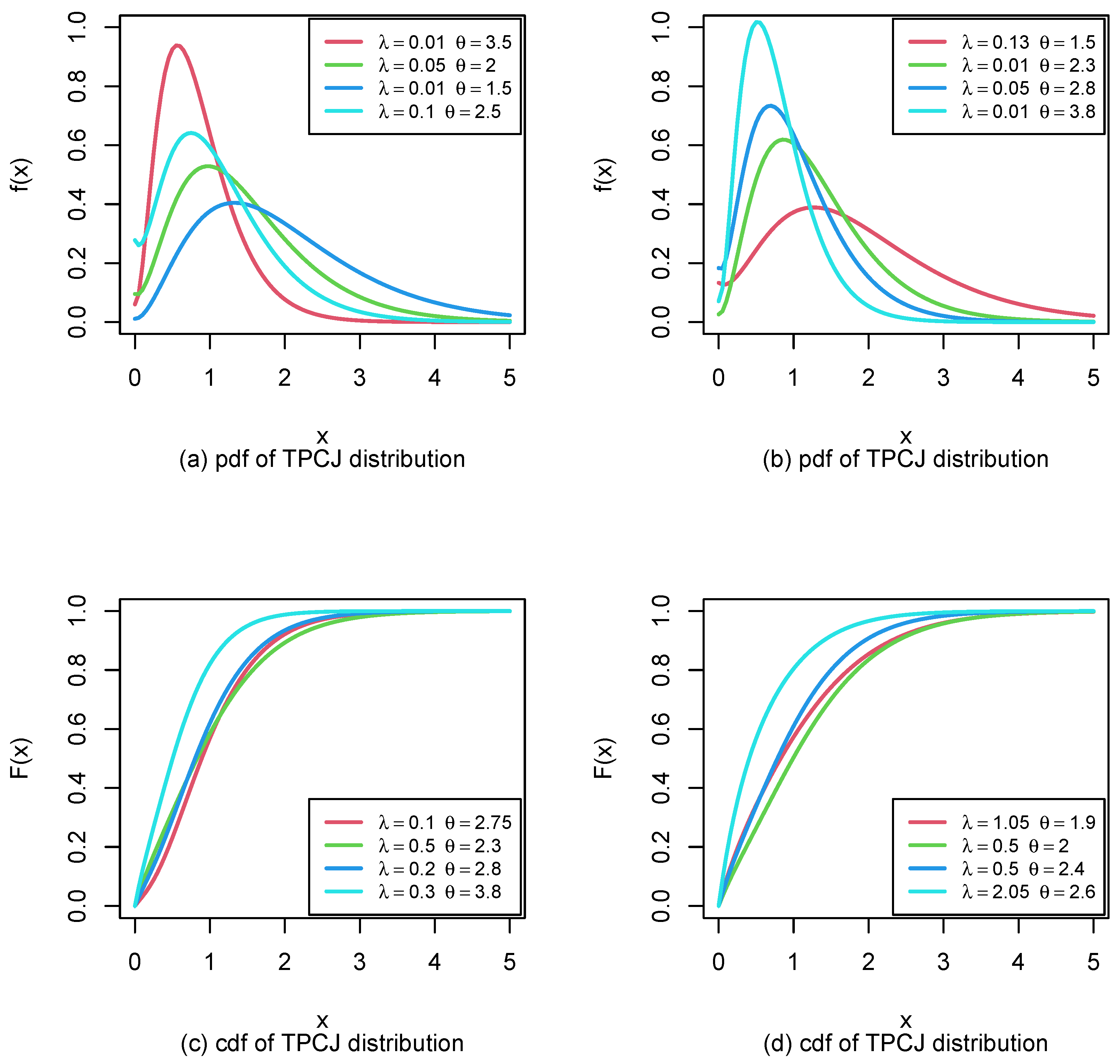
are the shape and scale parameters, respectively. The PDF and CDF plots are shown in
Figure 1.
The Reliability function of the TPCJD is
The Reliability function of the TPCJD is such that
and
. The hazard rate function of the TPCJD is
From the hazard rate function, it is easy to see that
- i.
.
- ii.
.
3. The Characteristics of the TPCJD
3.1. Complete Moment
The
rth crude moment of the TPCJD in the complete sense is given as
The first four non-central moments are obtained by replacing
r in (
7) by
respectively.
3.2. Variance of the TPCJD
In this subsection, the variance of the TPCJD is given by
The third and fourth central moments are respectively
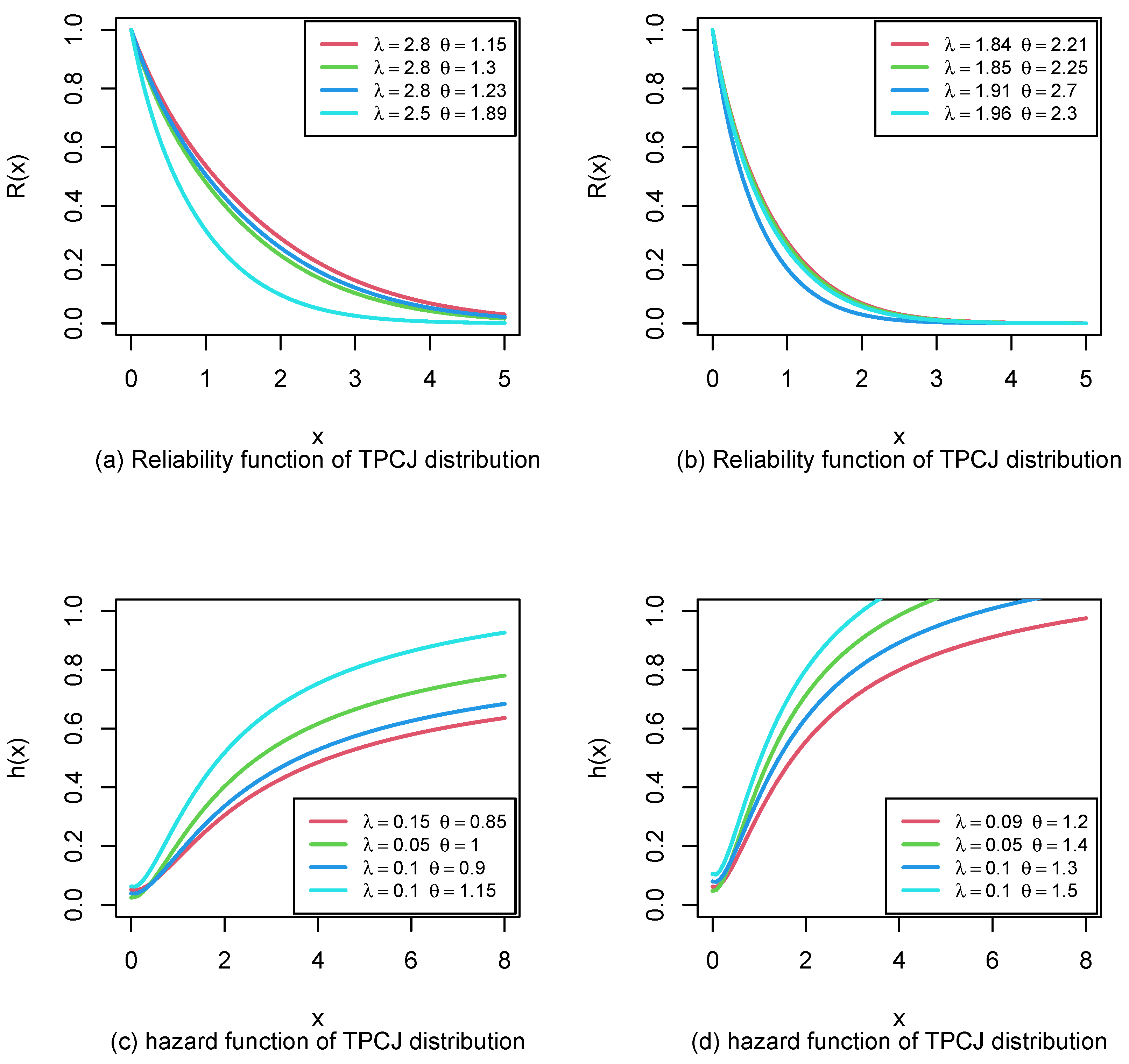
The survival and hazard functions plots are shown in
Figure 2.
Figure 2 provides useful insight into the behaviour of the TPCJD, having an increasing shape. Therefore, from
Figure 2, it is possible to model data sets with increasing failure rates with the TPCJD.
3.3. Skewness, Kurtosis, Coefficient of Variation, and Index of Dispersion
The moment coefficient of skewness, coefficient of kurtosis, coefficient of variation, and index of dispersion of the TPCJ distributed random variable
X are respectively given as
and
3.4. Moment-Generating Function of TPCJD
The moment-generating function of a
X ∼ TPCJ(
) is given by
The moment-generating function of the proposed TPCJD is defined only when .
3.5. Characteristic Function of TPCJD
The characteristic function of a
X ∼ TPCJ(
) is given by
3.6. The Order Statistics
The order statistics of the TPCJD are given by
and
are defined in Equations (
3) and (
4), respectively. Hence, we have
We obtain the PDF of the largest order statistics by substituting
in Equation (
17)
We obtain the PDF of the smallest order statistics by substituting
in Equation (
17)
3.7. Information Measure and the Behavior of TPCJD
Entropy is a measure of disorder in a system for a non-negative integer—say
. For
TPCJD, the Rény entropy is obtained as:
For
, we have the special case of Shannon Entropy
The asymptotic behavior of the TPCJ distributed random variable is obtained by taking the limit of the PDF as
and as
.
and
3.8. The Odds Function
The Odds function is a reliability tool for modelling a data set that shows a non-monotone hazard rate. It is defined to be the ratio of the CDF to the survival function
3.9. The Stress–Strength Reliability Analysis
The reliability of a system is a function of its strength. Therefore, when a higher stress exacts on the system, the system collapses and hence is not reliable. Suppose
TPCJD
and
TPCJD
are two independent continuous random variables representing the strength and stress of a system, respectively. Following that, the stress–strength reliability can be expressed as
where
is the joint probability density function of
Y and
X.
from basic knowledge of independence of two random variables
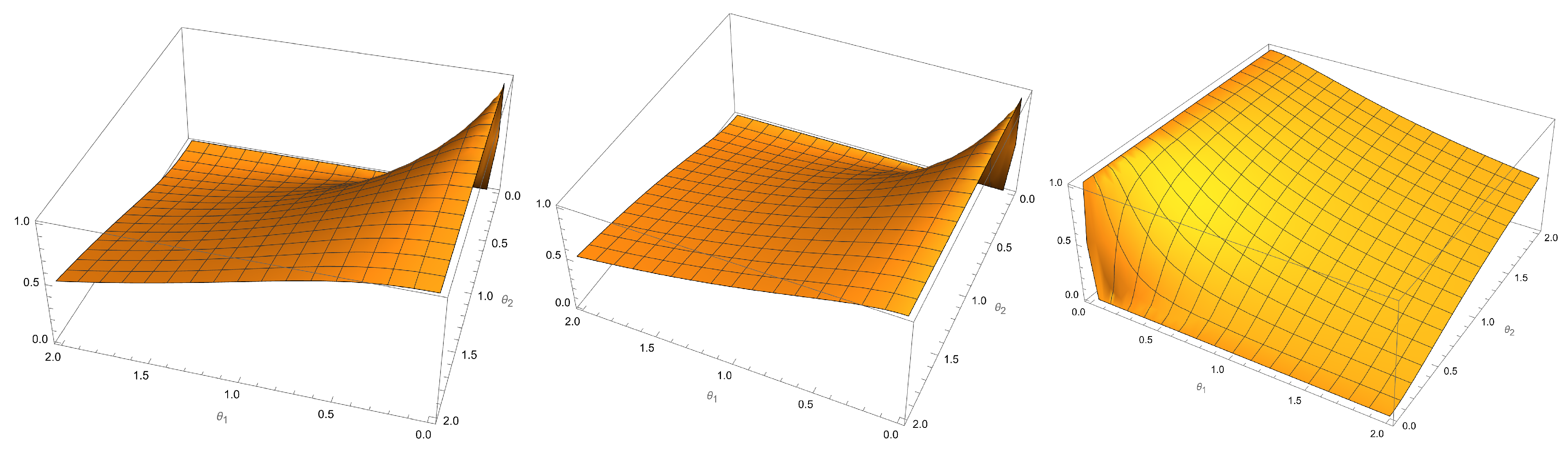
Figure 3 discusses stress–strength reliability plots with different parameters by using Equation (
28).
3.10. Maximum Likelihood Estimation of the TPCJD
Let
be
n random samples drawn from TPCJD, then the likelihood function is given as
Next, take the logarithm of
ℓ and differentiate partially with respect to
and
to obtain the following non-linear equations
Set
, which yields the following quadratic result
Set
, which yields the following quadratic result
Approximate Confidence Interval (ACI) of the MLEs
The approximate confidence intervals of the parameters are based on the asymptotic distribution of the maximum likelihood estimates of the u parameters
. The asymptotic variances and covariances of
and
are the elements of the inverse of the Fisher information matrix. Hence,
where
Therefore, a
approximate confidence intervals for
and
are, respectively,
follows the percentile standard normal distribution with right-tailed probability.
3.11. The Least Squares Estimation (LSE)
From Swain et al. [
17], we can derive the LSEs of the parameters
and
as follows:
Minimize the function
to obtain the estimates
and
of the parameters
and
as follows
Resolving the following non-linear systems of equations produces the estimates
where
More papers discussed these methods as [
18,
19].
3.12. The Weighted Least Squares Estimation (WLSE)
Minimize the function
to obtain the estimates
and
of the proposed TPCJD parameters
and
as follows
Resolving the following non-linear systems of equations produces the estimates
and
are respectively defined in (
40) and (
41).
3.13. The Maximum Product Spacing Estimators (MPSE)
The Kullback–Leibler measure is approximated by the maximum product spacing method and, of course, it is a good alternative method to the maximum likelihood. Considering increasing ordered data, the maximum product spacing for the TPCJD can be derived as follows
where
,
.
An alternative function to maximize in order to obtain the estimates is
For the first derivative, we solved the function and the associated nonlinear equations with respect to and . That is, = 0 and = 0, where , the estimates of the parameters are derived.
3.14. Cramér-Von-Mises Estimation (CVME)
We minimized the function
to obtain the estimates
, and
of the TPCJD parameters
, and
as follows
Resolving the following non-linear systems of equations produces the estimates
and
are, respectively, defined in (
40) and (
41).
3.15. The Anderson–Darling Estimation (ADE)
We minimized the function
to obtain the estimates
, and
of the TPCJD parameters
and
as follows
Resolving the following non-linear systems of equations produces the estimates
where
and
are as defined in (
40) and (
41), respectively.
3.16. The Right-Tailed Anderson–Darling Estimation (RTADE)
We minimized the function
to obtain the estimates
and
of the TPCJD parameters
and
as follows
Resolving the following non-linear systems of equations produces the estimates
and
are respectively defined in (
40) and (
41). We obtained the estimates in (
32), (
33), (
43), (
44), (
46), (
48), (
50), and (
52) by iterative algorithm in R.
3.17. The Tail Analysis of TPCJD
In this subsection, we zoomed into the tails of the TPCJD to investigate characteristics. Firstly, the ratio of the TPCJD’s survival function to that of the exponential survival function was investigated to ascertain the tail weight. This will give an idea of the speed of decay of the TPCJD’s survival function.
Secondly, the mean residual life function (or the mean excess loss function) was derived. This will provide the expected loss over a specified threshold, conditioned on the event that the threshold has already been exceeded.
Thirdly, we determined the maximum domain of attraction of TPCJD. Given that the extreme value theorem provides three extreme types (Gumbel, Frechet, and Weibull), the goal here is to ascertain which of the types the TPCJD tail falls into.
3.17.1. Comparing Tail Weights
The comparing tail weights are given by
Dividing through by
and taking limit as
The distribution of the TPCJD has a heavier tail than that of the exponential distribution.
3.17.2. The Mean Residual Life Function
The mean residual life function
is obtained as follows
Substituting into the formula, we obtain
3.17.3. The Domain of Attraction
For each of the Gumbel, Frechet, and Weibull distributions, known as the extreme value distributions, we briefly list the necessary and sufficient requirements that must be met for a distribution function to be a member of the maximum domain of attraction .
Theorem 1. Let the right extremity of F be given by
- (1)
- (2)
and
- (3)
and
By using the probability density function and distribution function in Equations (
3) and (
4), we call
the shape parameter and
the shape parameter of the TPCJD, respectively, and we can determine the domain of attraction for the TPCJD.
Making use of the necessary and sufficient conditions for Gumbel
Therefore, setting
and
Dividing through by
and taking limit as
As a result, the TPCJD falls under the Gumbel domain of attraction. The Gumbel domain of attraction is characterized by distributions with a significant range of tail heaviness and either infinite or finite upper endpoints.
4. Single Acceptance Sampling Plan (SASP) for TPCJD
Assume that the lifetime of a good is determined by the TPCJD, whose parameters are
, as stated in Equation (
3), and that the producer’s declared industry standard for the lifespan of units is symbolized by
. The primary objective is to decide whether or not to accept the proposed lot given that the actual median life cycle of the units,
m, is longer than the suggested lifetime,
. The test must be completed by the time provided by
in order to count the number of failures, which is typical practice in life testing.
Given the evidence that
, given a probability of at least
(consumer’s risk), utilizing a single acceptance sampling plan, Singh and Tripathi [
20] gave us some recommendations on how to accept the suggested lot. Additionally, Maya et al. [
21] developed a lifetime acceptance sampling plan and provided the HEB distribution. The experiment is conducted during a time period of
, which is longer than the claimed median lifetime with any positive constant
a. Steps:
Select a random sample of n units from the proposed lot.
Run the following evaluation for time units:
If c or fewer units (the acceptance number) fail over the course of the experiment, accept the entire lot; if not, reject the entire lot.
We note that the suggested sampling strategy is provided by and that the likelihood of accepting a lot takes into account suitable large lots to aid in the application of the binomial distribution.
According to Equaiton (
4),
is defined as
. The function
is used to represent the operational characteristic function of the sampling plan as well as the acceptance probability of the lot as a function of the failure probability. Using
,
can also be represented as follows:
Now, the problem is to determine for given values of
and
c, the smallest positive integer
n such that
where
is given by Equation (
60).
We make the following assumptions for the operating characteristic probability and the minimal values of
n, which satisfies the inequality in Equation (
61) as contained in
Table 1,
Table 2,
Table 3 and
Table 4:
For the operational characteristic probability and the minimal values of
n that satisfy the inequality in Equation (
61), as shown in
Table 1,
Table 2,
Table 3 and
Table 4: we make the following assumptions:
The risk for the consumer was set at , and .
The acceptance number c assumes the following values and 10.
The constant a takes the following values and . If , thus is the median life time ).
After trial and error, the following values are suitable for the parameters
of the TPCJD:
As , c, and the required sample size n increase, the decreases.
The needed sample size n reduces as a rises, whereas rises.
The needed sample size n increases and is lowers as increases and remains constant.
The needed sample size n grows and shrinks as increases and fixed remains constant.
Finally, for all scenarios, we verified that . Also, for as , hence in all results , for any values of the parameters considered are the same.
5. The Bayesian Estimation of the TPCJD Parameters
The parameters of the TPCJD’s Bayesian Estimates (BE) are derived in this section. There are three types of loss functions used: squared error, LINEX, and generalized entropy loss functions. The following independent gamma priors are utilized for
and
:
To represent the previous knowledge about the unknown parameters, the hyper-parameters
were used. The following is how we arrived at the joint prior for the parameter
.
The associated posterior density for the observed data
is given by:
Which implies that the posterior density function is:
The setting, the nature of the issue, and the decision-maker’s preferences on errors all affect the choice of loss function in Bayesian inference. While generalized entropy and linear-exponential losses offer more flexibility to address cases where different types of errors have variable effects, squared error loss is a popular and simple option. The relative costs or preferences associated with various outcomes are frequently taken into account while selecting a loss function that is compatible with real-world applications such as regression, risk assessment, and quality control for the squared error loss (SEL) function, medical diagnosis and finance for Linear-exponential loss (LINEX), economics and finance, environmental decision-making, and machine learning for the generalized entropy loss function. Given any function, such as
, under the squared error loss (SEL) function, the Bayes estimator is given by
In some cases, a proposed LINEX loss can be made instead of the SEL provided by
is a shape parameter.
indicates that an underestimation is milder than an overestimation and the reverse is the case for
. Moreover, when
, the SE loss function replicates itself. A detailed study is found in Varian [
22] and Doostparast et al. [
23]. The Bayes estimates of
under LINEX loss function are obtained as:
The third loss function is the general entropy loss (GEL) function proposed by Calabria and Pulcini [
24], and is given as follows.
where a break from symmetry is indicated by the shape parameter
. for
, it considers overestimation to be more significant than underestimation, and the opposite is true for
. The Bayes estimator for the GE loss function is provided.
It is clear that the estimations generated by (
65), (
66), and (
66) cannot be converted into closed-form expressions. Following that, in order to create posterior samples and produce appropriate Bayes estimates, we employed the Markov chain Monte Carlo (MCMC) method. In MCMC, a portion of the initial samples from the random samples of size
M derived from the posterior density can be discarded (burned in), and the remaining samples are then utilized to compute Bayes estimates. The BEs of
can be determined using MCMC under the SEL, LINEX, and GEL functions as follows:
is the number of burn-in samples. Read Ravenzwaaij et al. [
25] for further details on MCMC.
Credible Intervals for Bayes Estimates
A
credible intervals for the parameters
under the loss functions discussed are
is distributed according to percentile standard normal with right-tailed probability.
6. Simulation Study
In this section, we simulated data for the TPCJD to show how each of the non-Bayesian estimation methods performed. First, 1000 data points were generated from the TPCJD by considering the initial parameter values as
and
and
and
and
and sample sizes
. For each estimate
, the Bias and Root Mean Squared Error (RMSE) were calculated, respectively, as
and
To locate the desired estimates for the non-Bayesian process, we employed the Newton–Raphson algorithm. With the Bayesian approach, BEs are generated while accounting for prior knowledge using MCMC and the MH algorithm. We made the gamma distribution hyper-parameters for the prior data equal to double the parameter values. These values were filled in to provide the estimates we were looking for. The maximum likelihood estimates take initial guess values into consideration by using the MH method. In order to acquire the Bayes estimates under SEL, LINEX at , and the GEL at , we finally eliminate 2000 burn-in samples from the overall 10,000 samples produced from the posterior density. We calculate the bias and RMSE for each strategy. For the MCMC method, there are two types of graphs: marginal posterior and cumulative sum plots for lambda and theta. It is evident that the MCMC is a reliable method that, after a 5000 burn-in from a 10,000 sample draw, meets stability and convergences.
As the sample size increases, we occasionally observe a decrease in the Bias and RMSE for all estimations.
This indicates that using a variety of estimation techniques yields reliable Bias and RMSE results for big sample sizes.
The MPSE estimate method offers better metrics than the LSE, WLSE, CVME, ADE, and RTADE approaches.
All estimators’ Bias and RMSE values decrease as sample size rises, indicating improved model parameter estimation accuracy.
LSE, WLSE, CVME, ADE, and RTADE are the parameters that are least biased when compared to all other parameters and different sample sizes.
All sample sizes have a positive estimators’ bias.
From
Table 5,
Table 6,
Table 7,
Table 8 and
Table 9, we noted that the WLSE, LSE, CVME, ADE, RTADE, MLE, and Bayesian methods, respectively, give smaller values for accurate Bias and RMSE findings for large sample sizes.
7. Applications
In this section, the performance of the TPCJD is illustrated using two life data sets.
7.1. Application to Infant Mortality Rate Data
The first set of information is a description of the infant mortality rate per 1000 live births for a few chosen nations in 2021, as reported by a
https://data.worldbank.org/indicator/SP.DYN.IMRT.IN (accessed on 2021). This real data set is presented as
| 56 | 10 | 22 | 3 | 69 | 6 | 7 | 11 | 4 | 4 | 19 | 13 | 7 | 27 | 12 | 3 | 4 | 11 |
| 84 | 27 | 25 | 6 | 35 | 14 | 11 | 12 | 6 | | | | | | | | | |
Here, we compare the goodness of fit of the TPCJD with the Burr III distribution by Papadopoulos [
26], Exponentiated Inverse Exponential (EIE) by [
27], Weibull distribution, Gamma distribution, Lomax distribution, and the parent distribution called C-JD by Onyekwere and Obulezi [
2], as shown in
Table 10. The fitness metrics considered are the Negative log-likelihood (NLL), the Akaike information criterion (AIC), the corrected AIC (CAIC), the Bayesian information criterion (BIC), the Hannan–Quinn information criterion (HQIC), Anderson Darling (AD), and Cramér-von-Mises (CVM) statistics. The model with the lowest values of these metrics is chosen as the best performer.
The fitness criterion states that the distribution that fits the data the best and has a
p-value larger than
meets the requirement for fitness. The infant mortality rate is best suited by the proposed TPCJD, according to the findings in
Table 10.
The TPCJD has the smallest values of the Negative Log-Likelihood (NLL), Akaike information criterion (AIC), Corrected AIC (CAIC), Bayesian information criterion (BIC), Hannan–Quinn information criterion (HQIC), Anderson–Darling and Cramer Van Miss, and Kolmogorov–Smirnov (K–S) statistics, and hence performs better with the infant mortality rate data compared to TPOD, OGE, Burr, GIE, EIE, and C-J, as shown in
Table 10. The MLEs of the parameters of the fitted distributions are determined in
Table 11. The standard error (Std. Error) and classical and Bayesian estimates for the TPCJD’s parameters are also provided in
Table 11.
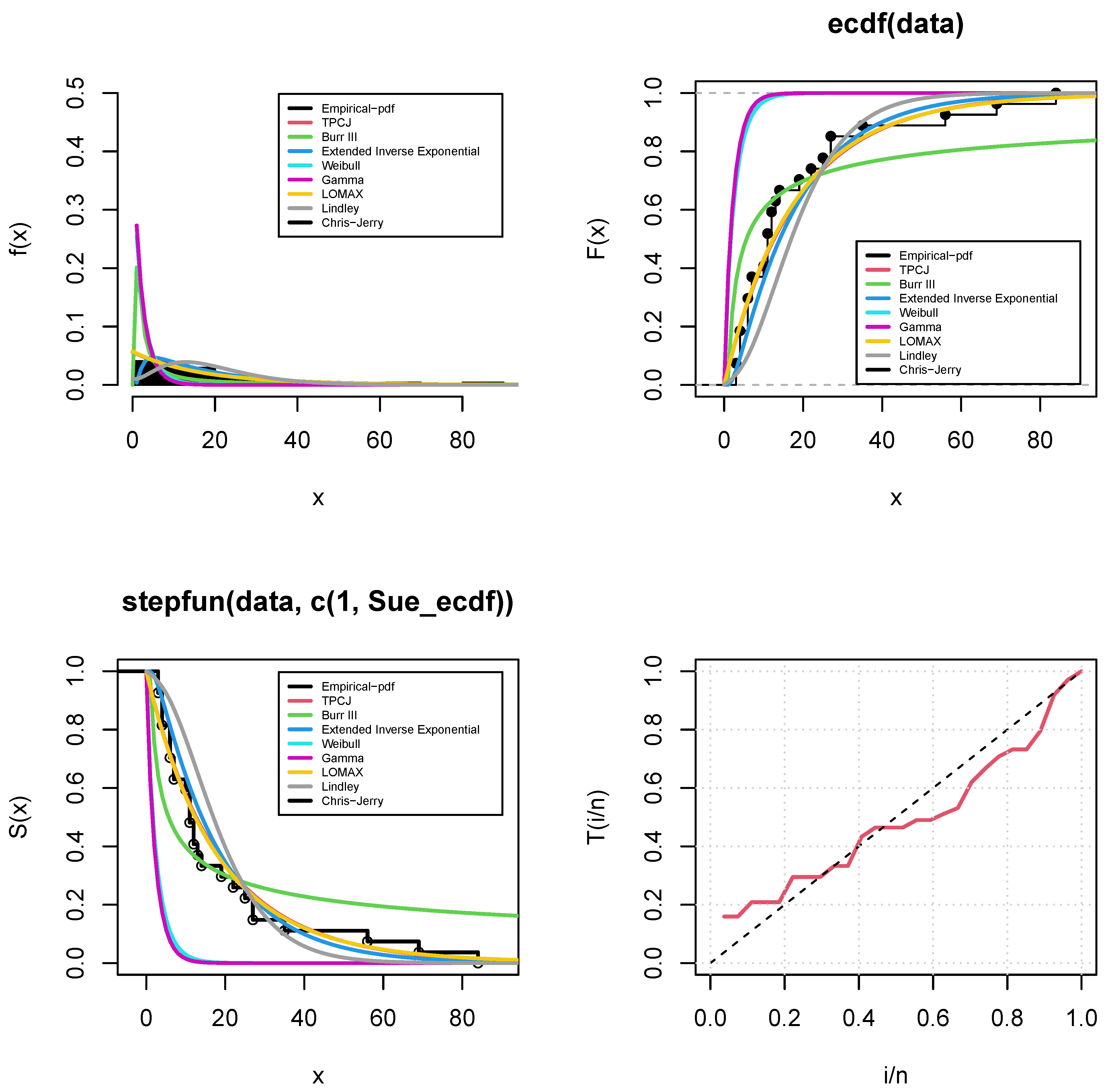
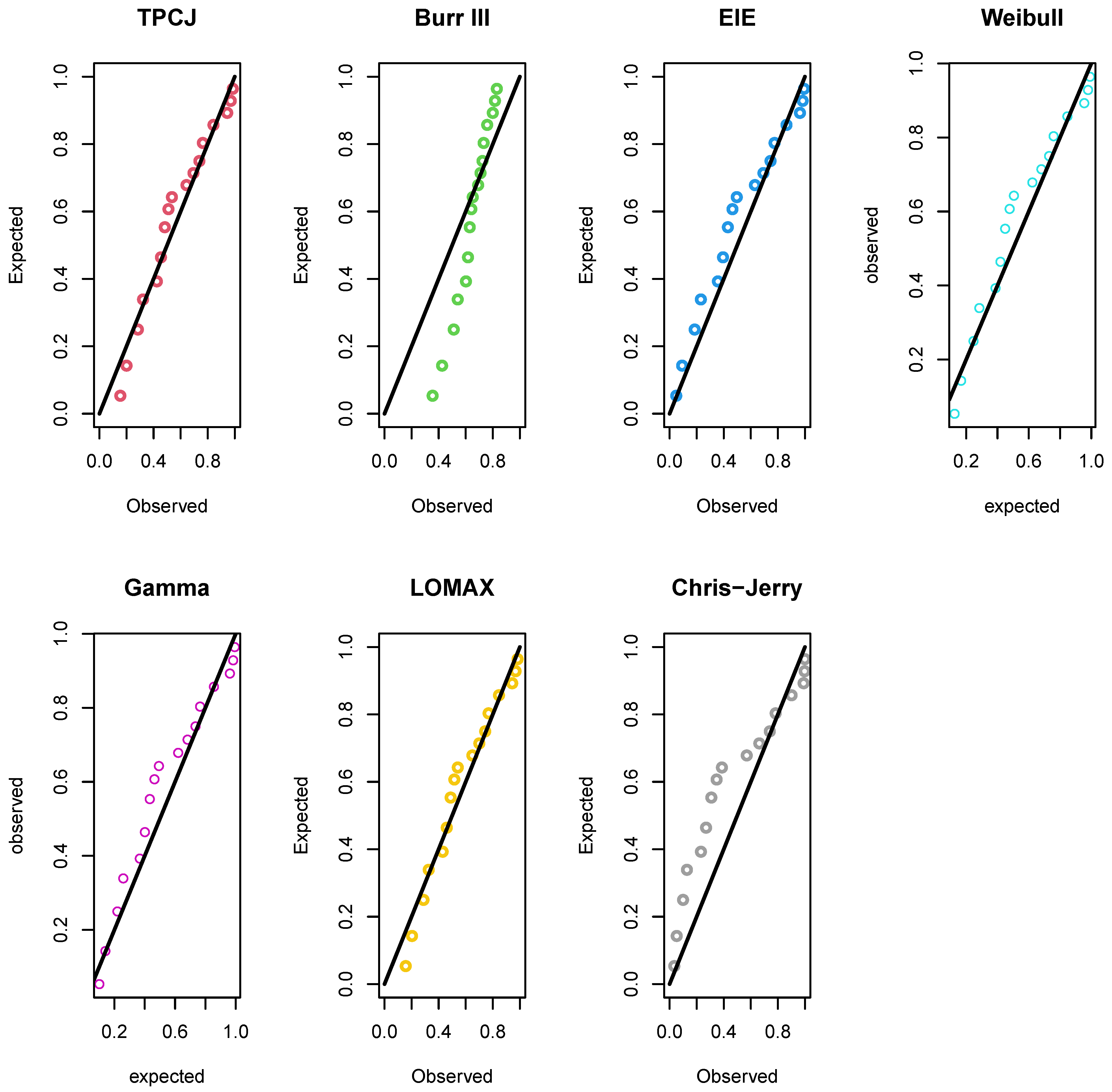
Figure 4 shows the fitted density, CDF, and empirical Survival function for the underlying TPCJD. In contrast,
Figure 5 is the PP plot of the fitted distributions using the infant mortality rate data. For the operational characteristic probability and the minimal values of
n for data on infant mortality rates, we use the following assumptions; for more information, see
Table 12.
Given that the model is the best match among competing distributions, the model performance measurements for the TPCJD in
Table 10 raise several questions. Other techniques were employed to estimate the parameters in order to assess the MLE method’s appropriateness. The Weighted Least Squares Estimates (WLSE) approach is the most effective, as shown in
Table 11. This is a result of these estimates’ minimum standard errors. In addition to the fact that the proposed TPCJD fits the infant mortality rate data better than the traditional Weibull, Gamma, Lomax, Exponentiated Inverse Exponential, Burr III, and the C-JD, maximum likelihood estimation is not a good estimation procedure for estimating the parameters of the TPCJD.
7.2. Application to Data on Life of Fatigue Fracture of Kevlar 373/epoxy
The application is on the life of fatigue fracture of Kevlar 373/epoxy subjected to constant pressure at
stress level until all had failed, as shown in
Table 13 (see Andrews and Herzberg [
28]).
In
Table 14, by comparing the proposed TPCJD’s goodness of fit to that of the Burr, EIE, Weibull, GIE, Lomax, and C-J distributions at the instance of the time to the breakdown of an insulating fluid between electrodes at a voltage of 34 k.v. (minutes) data, we are able to demonstrate the suggested TPCJ distribution’s use. The measurements of fitness include Kolmogorov–Smirnov (K–S) statistics, Akaike information criterion (AIC), Corrected AIC (CAIC), Bayesian information criterion (BIC), Anderson–Darling (AD), Cramer von Mises (CVM), and Negative Log-Likelihood (NLL). The model with the fewest indices meets the performance criterion.
The fitness criterion states that the distribution that fits the data the best and has a
p-value larger than
meets the requirement for fitness. According to the results in
Table 14, the proposed TPCJD fits the data for the most optimal time taken for an insulating fluid between electrodes to break down at a voltage of 34 k.v.
The Bayes Estimates (BE) and Weighted Least Squares Estimates (WLSE) outperformed the others, as shown in
Table 15. This is a result of these estimates’ minimum standard errors. The standard error (Std. ErrorS) and classical and Bayesian estimates for the TPCJD’s parameters are provided in
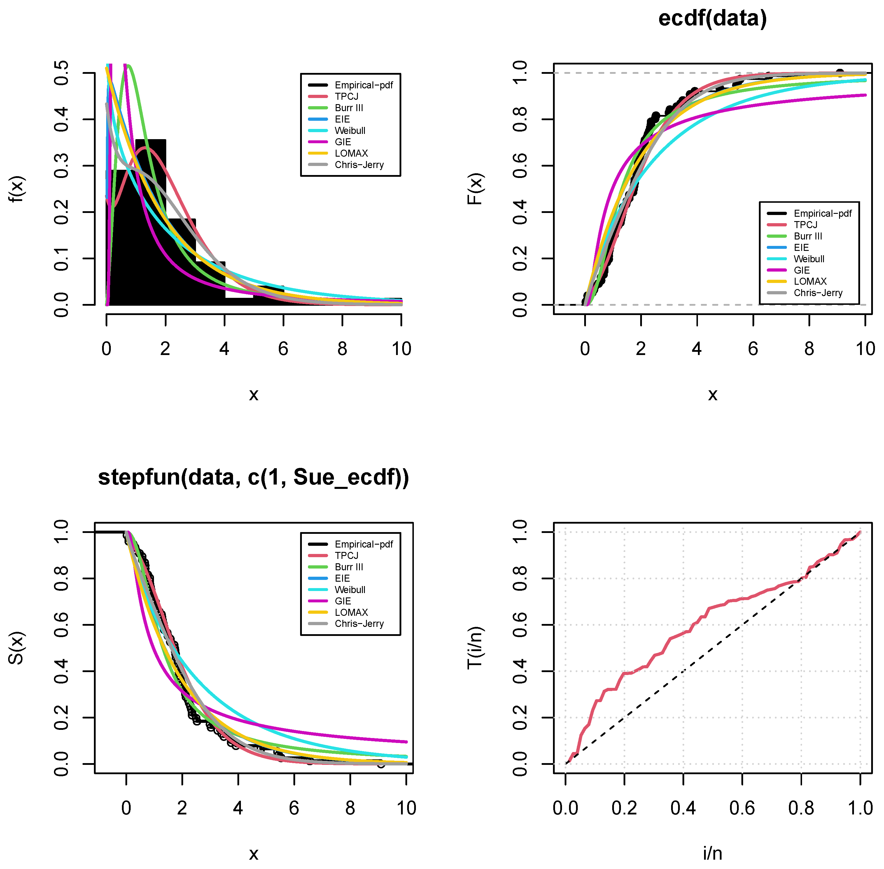
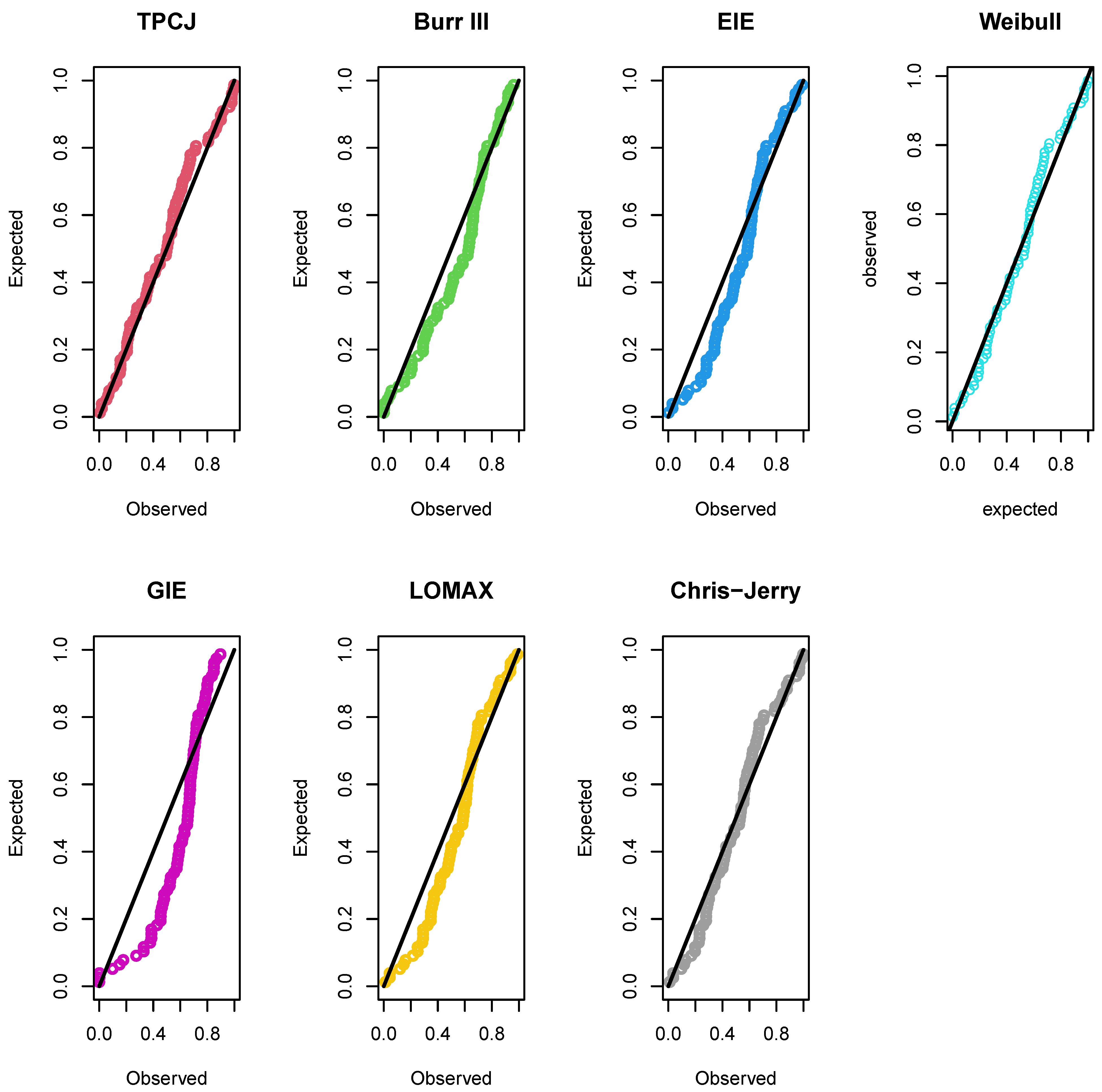
Table 15. The density, CDF, empirical reliability, and PP plots of the fitted distributions of the time to break down an insulating fluid between electrodes at 34 k.v. (minutes) data are presented in
Figure 6 and
Figure 7, respectively, for the underlying TPCJD. For the operating characteristic probability and the minimal values of
n for fluid between electrodes at a voltage of 34 k.v. (minutes) data, see
Table 16, we adopt the following assumptions.
8. Conclusions
A new life distribution, named the two-parameter Chris-Jerry distribution (TPCJD), has been proposed and studied here. The characteristics of the proposed distribution, moments, moment-generating function, and order statistics are derived. The MLEs, LSEs, WLSEs, CVMEs, ADEs, and RTADEs were derived and implemented. Bayesian inference with squared error loss, linear exponential loss, and generalized entropy loss functions were also studied, and the simulation of parameters based on the classical and Bayesian methods was carried out. Also, the asymptotic confidence intervals and credible intervals for the maximum likelihood estimates and Bayesian estimates were obtained. Applications to lifetime data using the infant mortality rate per 1000 live births for some selected countries in the year 2021 and the time to break down an insulating fluid between electrodes at 34 k.v. (minutes) data were also illustrated. From the metrics of fitness (K-S and p-value) and performance indices (LL, AD, CVM, AIC, CAIC, BIC, HQIC), the proposed TPCJD is better than the following fitted distributions: Burr distribution, Generalized Inverse Exponential (GIE) distribution, Exponentiated Inverse Exponential (EIE), Weibull, Gamma, Lomax, and Chris-Jerry distribution (C-JD).
9. Future Work
Further study on the proposed distribution can explore more characterizations, namely the normalized incomplete moment, conditional value at risk, buffered probability of exceedance, and Pietra and Gini indices for measuring income and population inequalities.
Author Contributions
Conceptualization, O.J.O.; Methodology, A.H.T., E.Q.C., N.A. and O.J.O.; Software, A.H.T., E.M.A. and O.J.O.; Validation, Q.C.C. and O.J.O.; Formal analysis, E.M.A. and A.H.T.; Investigation, Q.C.C., E.Q.C. and N.A.; Resources, A.H.T. and O.J.O.; Data curation, N.A., E.M.A., O.J.O. and A.H.T.; Writing—original draft, A.H.T., E.M.A., Q.C.C., E.Q.C. and O.J.O.; Writing—review & editing, A.H.T. and O.J.O.; funding acquisition N.A. All authors have read and agreed to the published version of the manuscript.
Funding
This research is supported by researchers supporting project number (RSPD2023R548), King Saud University, Riyadh, Saudi Arabia.
Data Availability Statement
Not applicable.
Conflicts of Interest
The authors declare no conflict of interest.
References
- Lindley, D.V. Fiducial distributions and Bayes’ theorem. J. R. Stat. Soc. Ser. B Methodol. 1958, 20, 102–107. [Google Scholar] [CrossRef]
- Onyekwere, C.K.; Obulezi, O.J. Chris-Jerry Distribution and Its Applications. Asian J. Probab. Stat. 2022, 20, 16–30. [Google Scholar] [CrossRef]
- Odom, C.C.; Ijomah, M.A. Odoma distribution and its application. Asian J. Probab. Stat. 2019, 4, 1–11. [Google Scholar] [CrossRef]
- Tolba, A.H.; Almetwally, E.M. Bayesian and Non-Bayesian Inference for The Generalized Power Akshaya Distribution with Application in Medical. Comput. J. Math. Stat. Sci. 2023, 2, 31–51. [Google Scholar]
- Tolba, A. Bayesian and Non-Bayesian Estimation Methods for Simulating the Parameter of the Akshaya Distribution. Comput. J. Math. Stat. Sci. 2022, 1, 13–25. [Google Scholar] [CrossRef]
- Obulezi, O.J.; Anabike, I.C.; Oyo, O.G.; Igbokwe, C.P. Marshall-Olkin Chris-Jerry Distribution and its Applications. Int. J. Innov. Sci. Res. Technol. 2023, 8, 522–533. [Google Scholar]
- Shukla, K.K. Pranav distribution with properties and its applications. Biom. Biostat. Int. J. 2018, 7, 244–254. [Google Scholar]
- Shanker, R.; Shukla, K.K.; Shanker, R.; Pratap, A. A generalized Akash distribution. Biom. Biostat. Int. J. 2018, 7, 18–26. [Google Scholar] [CrossRef]
- Shanker, R. Sujatha distribution and its Applications. Stat. Transit. New Ser. 2016, 17, 391–410. [Google Scholar] [CrossRef]
- Bjerkedal, T. Acquisition of Resistance in Guinea Pies infected with Different Doses of Virulent Tubercle Bacilli. Am. J. Hyg. 1960, 72, 130–148. [Google Scholar] [PubMed]
- Yahaya, A.; Abdullahi, J. Theoretical Study of Four-Parameter Odd-Generalized Exponential-Pareto Distribution. Ann. Stat. Theory Appl. ASTA 2019, 2, 103–114. [Google Scholar]
- Enogwe, S.U.; Nwosu, D.F.; Ngome, E.C.; Onyekwere, C.K.; Omeje, I.L. Two-parameter Odoma distribution with applications. J. Xidian Univ. 2020, 14, 740–764. [Google Scholar]
- Abouammoh, A.M.; Alshingiti, A.M. Reliability estimation of generalized inverted exponential distribution. J. Stat. Comput. Simul. 2009, 79, 1301–1315. [Google Scholar] [CrossRef]
- Shukla, K.K.; Shanker, R. Shukla distribution and its Application. Reliab. Theory Appl. 2019, 14, 46–55. [Google Scholar]
- Umeh, E.; Ibenegbu, A. A Two-Parameter Pranav Distribution with Properties and Its Application. J. Biostat. Epidemiol. 2019, 5, 74–90. [Google Scholar] [CrossRef]
- Shukla, K.K. Inverse Ishita Distribution: Properties and Applications. Reliab. Theory Appl. 2021, 16, 98–108. [Google Scholar]
- Swain, J.J.; Venkatraman, S.; Wilson, J.R. Least-squares estimation of distribution functions in Johnson’s translation system. J. Stat. Comput. Simul. 1988, 29, 271–291. [Google Scholar] [CrossRef]
- Shakil, M.; Munir, M.; Kausar, N.; Ahsanullah, M.; Khadim, A.; Sirajo, M.; Singh, J.N.; Kibria, B.M.G. Some Inferences on Three Parameters Birnbaum-Saunders Distribution: Statistical Properties, Characterizations and Applications. Comput. J. Math. Stat. Sci. 2023, 2, 197–222. [Google Scholar] [CrossRef]
- Abubakari, A.G.; Anzagra, L.; Nasiru, S. Chen Burr-Hatke exponential distribution: Properties, regressions and biomedical applications. Comput. J. Math. Stat. Sci. 2023, 2, 80–105. [Google Scholar] [CrossRef]
- Singh, S.; Tripathi, Y.M. Acceptance sampling plans for inverse Weibull distribution based on truncated life test. Life Cycle Reliab. Saf. Eng. 2017, 6, 169–178. [Google Scholar] [CrossRef]
- Maya, R.; Irshad, M.R.; Ahammed, M.; Chesneau, C. The Harris Extended Bilal Distribution with Applications in Hydrology and Quality Control. Appl. Math. 2023, 3, 221–242. [Google Scholar] [CrossRef]
- Varian, H.R. A Bayesian approach to real estate assessment. In Studies in Bayesian Econometric and Statistics in Honor of Leonard J. Savage; North Holland: Amsterdam, The Netherlands, 1975; pp. 195–208. [Google Scholar]
- Doostparast, M.; Akbari, M.G.; Balakrishna, N. Bayesian analysis for the two-parameter Pareto distribution based on record values and times. J. Stat. Comput. Simul. 2011, 81, 1393–1403. [Google Scholar] [CrossRef]
- Calabria, R.; Pulcini, G. Point estimation under asymmetric loss functions for left-truncated exponential samples. Commun. Stat. Theory Methods 1996, 25, 585–600. [Google Scholar] [CrossRef]
- Ravenzwaaij, D.V.; Cassey, P.; Brown, S.D. A simple introduction to Markov Chain Monte–Carlo sampling. Psychon. Bull. Rev. 2018, 25, 143–154. [Google Scholar] [CrossRef] [PubMed]
- Papadopoulos, A.S. The Burr distribution as a failure model from a Bayesian approach. IEEE Trans. Reliab. 1978, 27, 369–371. [Google Scholar] [CrossRef]
- Fatima, K.; Ahmad, S.P. The Exponentiated Inverted Exponential Distribution. J. Appl. Inf. Sci. Vol. 2017, 5, 36–41. [Google Scholar]
- Andrews, D.F.; Herzberg, A.M. Stress-rupture life of kevlar 49/epoxy spherical pressure vessels. Data 1985, 181–186. [Google Scholar]
Figure 1.
TPCJD’s pdf and the cdf plots.
Figure 1.
TPCJD’s pdf and the cdf plots.
Figure 2.
Reliability rate and hazard rate functions of the TPCJD.
Figure 2.
Reliability rate and hazard rate functions of the TPCJD.
Figure 3.
Stress–strength reliability plots with different parameters.
Figure 3.
Stress–strength reliability plots with different parameters.
Figure 4.
Statistical fitting of distributions to the world infant mortality rate per 1000 live birth data using empirical PDF, CDF, and survival plots.
Figure 4.
Statistical fitting of distributions to the world infant mortality rate per 1000 live birth data using empirical PDF, CDF, and survival plots.
Figure 5.
The PP plots of the distributions fitted to the world infant mortality rate per 1000 live birth data.
Figure 5.
The PP plots of the distributions fitted to the world infant mortality rate per 1000 live birth data.
Figure 6.
Using data on the amount of time needed for an insulating fluid between electrodes to break down at a voltage of 34 k.v., empirical PDF, CDF, and survival plots of fitted distribution were plotted.
Figure 6.
Using data on the amount of time needed for an insulating fluid between electrodes to break down at a voltage of 34 k.v., empirical PDF, CDF, and survival plots of fitted distribution were plotted.
Figure 7.
The fitted distributions’ PP graphs using the measured data for the number of minutes it takes for an insulating fluid between electrodes to break down at a voltage of 34 k.v.
Figure 7.
The fitted distributions’ PP graphs using the measured data for the number of minutes it takes for an insulating fluid between electrodes to break down at a voltage of 34 k.v.
Table 1.
The SASP for the TPCJD with parameter: for different values of .
Table 1.
The SASP for the TPCJD with parameter: for different values of .
| * | c | | | | | |
|---|
| | | | | | | | | |
|---|
| | | | | | | | | | | |
| 0.25 | 0 | 49 | 0.75124 | 13 | 0.76046 | 3 | 0.81034 | 1 | 1 | 1 | 1 |
| | 2 | 291 | 0.75137 | 77 | 0.75423 | 18 | 0.76268 | 5 | 0.86067 | 4 | 0.87500 |
| | 4 | 568 | 0.75034 | 150 | 0.75264 | 35 | 0.75164 | 10 | 0.80543 | 8 | 0.77344 |
| | 8 | 1152 | 0.75035 | 304 | 0.75190 | 70 | 0.75151 | 20 | 0.77993 | 15 | 0.78802 |
| | 10 | 1452 | 0.75037 | 383 | 0.75194 | 88 | 0.75095 | 25 | 0.77799 | 19 | 0.75966 |
| 0.75 | 0 | 233 | 0.25096 | 61 | 0.25431 | 14 | 0.25488 | 4 | 0.25836 | 2 | 0.50000 |
| | 2 | 659 | 0.25082 | 173 | 0.25280 | 39 | 0.25487 | 10 | 0.30751 | 7 | 0.34375 |
| | 4 | 1055 | 0.25069 | 277 | 0.25268 | 62 | 0.25914 | 17 | 0.25304 | 12 | 0.27441 |
| | 8 | 1817 | 0.25046 | 478 | 0.25084 | 107 | 0.25796 | 29 | 0.26007 | 21 | 0.25172 |
| | 10 | 2190 | 0.25046 | 576 | 0.25109 | 129 | 0.25821 | 35 | 0.25863 | 25 | 0.27063 |
| 0.95 | 0 | 503 | 0.05022 | 132 | 0.05032 | 29 | 0.05264 | 7 | 0.06675 | 5 | 0.06250 |
| | 2 | 1058 | 0.05012 | 277 | 0.05075 | 61 | 0.05352 | 16 | 0.05028 | 11 | 0.05469 |
| | 4 | 1539 | 0.05002 | 404 | 0.05009 | 90 | 0.05026 | 23 | 0.05612 | 16 | 0.05923 |
| | 8 | 2427 | 0.05005 | 637 | 0.05032 | 142 | 0.05089 | 37 | 0.05293 | 26 | 0.05388 |
| | 10 | 2852 | 0.05007 | 749 | 0.05017 | 167 | 0.05096 | 43 | 0.06059 | 30 | 0.06802 |
| | | | | | | | | | | |
| 0.25 | 0 | 41 | 0.75452 | 12 | 0.76285 | 3 | 0.80668 | 1 | 1 | 1 | 1 |
| | 2 | 247 | 0.75056 | 72 | 0.75130 | 18 | 0.75314 | 5 | 0.85996 | 4 | 0.87500 |
| | 4 | 481 | 0.75050 | 139 | 0.75409 | 34 | 0.75812 | 10 | 0.80417 | 8 | 0.77344 |
| | 8 | 976 | 0.75002 | 282 | 0.75275 | 68 | 0.76011 | 20 | 0.77799 | 15 | 0.78802 |
| | 10 | 1230 | 0.75009 | 356 | 0.75085 | 86 | 0.75429 | 25 | 0.77582 | 19 | 0.75966 |
| 0.75 | 0 | 197 | 0.25153 | 57 | 0.25207 | 13 | 0.27555 | 4 | 0.25751 | 2 | 0.50000 |
| | 2 | 558 | 0.25080 | 161 | 0.25119 | 38 | 0.25856 | 10 | 0.30596 | 7 | 0.34375 |
| | 4 | 894 | 0.25004 | 257 | 0.25295 | 61 | 0.25591 | 17 | 0.25118 | 12 | 0.27441 |
| | 8 | 1539 | 0.25005 | 443 | 0.25230 | 105 | 0.25646 | 29 | 0.25759 | 21 | 0.25172 |
| | 10 | 1854 | 0.25056 | 535 | 0.25021 | 127 | 0.25272 | 35 | 0.25591 | 25 | 0.27063 |
| 0.95 | 0 | 426 | 0.05015 | 122 | 0.05092 | 28 | 0.05501 | 7 | 0.06631 | 5 | 0.06250 |
| | 2 | 896 | 0.05002 | 257 | 0.05077 | 60 | 0.05252 | 15 | 0.06899 | 11 | 0.05469 |
| | 4 | 1302 | 0.05020 | 374 | 0.05075 | 88 | 0.05083 | 23 | 0.05537 | 16 | 0.05923 |
| | 8 | 2054 | 0.05016 | 591 | 0.05037 | 139 | 0.05121 | 37 | 0.05201 | 26 | 0.05388 |
| | 10 | 2414 | 0.05014 | 695 | 0.05018 | 163 | 0.05254 | 43 | 0.05949 | 30 | 0.06802 |
Table 2.
The SASP for the TPCJD with parameters: for different values of .
Table 2.
The SASP for the TPCJD with parameters: for different values of .
| * | c | | | | | | |
|---|
| | | | | | | | | | | |
| | | | | | | | | | | | |
| 0.25 | 0 | | 27 | 0.75694 | 10 | 0.75867 | 3 | 0.79430 | 1 | 1 | 1 | 1 |
| | 2 | | 163 | 0.75079 | 58 | 0.75240 | 17 | 0.75099 | 5 | 0.85753 | 4 | 0.87500 |
| | 4 | | 317 | 0.75104 | 112 | 0.75444 | 32 | 0.75653 | 10 | 0.79982 | 8 | 0.77344 |
| | 8 | | 643 | 0.75059 | 227 | 0.75326 | 64 | 0.75693 | 20 | 0.77131 | 15 | 0.78802 |
| | 10 | | 810 | 0.75100 | 286 | 0.75316 | 80 | 0.76251 | 25 | 0.76829 | 19 | 0.75966 |
| 0.75 | 0 | | 130 | 0.25117 | 46 | 0.25134 | 13 | 0.25113 | 4 | 0.25461 | 3 | 0.25000 |
| | 2 | | 368 | 0.25007 | 129 | 0.25356 | 36 | 0.25115 | 10 | 0.30069 | 7 | 0.34375 |
| | 4 | | 588 | 0.25110 | 207 | 0.25176 | 57 | 0.25747 | 16 | 0.30450 | 12 | 0.27441 |
| | 8 | | 1013 | 0.25062 | 357 | 0.25009 | 98 | 0.25968 | 28 | 0.29459 | 21 | 0.25172 |
| | 10 | | 1221 | 0.25058 | 430 | 0.25075 | 119 | 0.25157 | 34 | 0.28766 | 25 | 0.27063 |
| 0.95 | 0 | | 280 | 0.05038 | 98 | 0.05096 | 27 | 0.05009 | 7 | 0.06483 | 5 | 0.06250 |
| | 2 | | 589 | 0.05033 | 207 | 0.05018 | 56 | 0.05299 | 15 | 0.06663 | 11 | 0.05469 |
| | 4 | | 857 | 0.05022 | 301 | 0.05027 | 82 | 0.05190 | 23 | 0.05289 | 16 | 0.05923 |
| | 8 | | 1352 | 0.05020 | 475 | 0.05030 | 130 | 0.05123 | 36 | 0.06152 | 26 | 0.05388 |
| | 10 | | 1589 | 0.05019 | 558 | 0.05054 | 153 | 0.05105 | 43 | 0.05585 | 30 | 0.06802 |
| | | | | | | | | | | | |
| 0.25 | 0 | | 24 | 0.75487 | 9 | 0.76668 | 3 | 0.78919 | 1 | 1 | 1 | 1 |
| | 2 | | 143 | 0.75091 | 54 | 0.75018 | 16 | 0.76950 | 5 | 0.85651 | 4 | 0.87500 |
| | 4 | | 278 | 0.75119 | 104 | 0.75274 | 31 | 0.76114 | 10 | 0.79798 | 8 | 0.77344 |
| | 8 | | 564 | 0.75041 | 210 | 0.75386 | 62 | 0.76283 | 20 | 0.76848 | 15 | 0.78802 |
| | 10 | | 711 | 0.75004 | 265 | 0.75218 | 78 | 0.76237 | 25 | 0.76510 | 19 | 0.75966 |
| 0.75 | 0 | | 114 | 0.25118 | 42 | 0.25624 | 12 | 0.27195 | 4 | 0.25341 | 3 | 0.25000 |
| | 2 | | 322 | 0.25122 | 120 | 0.25027 | 35 | 0.25250 | 10 | 0.29850 | 7 | 0.34375 |
| | 4 | | 516 | 0.25029 | 191 | 0.25382 | 56 | 0.25062 | 16 | 0.30167 | 12 | 0.27441 |
| | 8 | | 888 | 0.25062 | 330 | 0.25092 | 96 | 0.25369 | 28 | 0.29087 | 21 | 0.25172 |
| | 10 | | 1070 | 0.25093 | 398 | 0.25018 | 116 | 0.25081 | 34 | 0.28361 | 25 | 0.27063 |
| 0.95 | 0 | | 246 | 0.05001 | 91 | 0.05034 | 26 | 0.05185 | 7 | 0.06422 | 5 | 0.06250 |
| | 2 | | 516 | 0.05042 | 191 | 0.05071 | 55 | 0.05088 | 15 | 0.06566 | 11 | 0.05469 |
| | 4 | | 751 | 0.05026 | 278 | 0.05065 | 80 | 0.05133 | 23 | 0.05188 | 16 | 0.05923 |
| | 8 | | 1185 | 0.05019 | 439 | 0.05056 | 127 | 0.05002 | 36 | 0.06007 | 26 | 0.05388 |
| | 10 | | 1393 | 0.05010 | 516 | 0.05060 | 149 | 0.05105 | 43 | 0.05438 | 30 | 0.06802 |
Table 3.
The SASP for the TPCJD with parameters: for different values of .
Table 3.
The SASP for the TPCJD with parameters: for different values of .
| * | c | | | | | | |
|---|
| | | | | | | | | | | |
| | | | | | | | | | | | |
| 0.25 | 0 | | 32 | 0.75278 | 11 | 0.75491 | 3 | 0.79952 | 1 | 1 | 1 | 1 |
| | 2 | | 190 | 0.75135 | 63 | 0.75330 | 17 | 0.76393 | 5 | 0.85857 | 4 | 0.87500 |
| | 4 | | 370 | 0.75123 | 122 | 0.75427 | 33 | 0.75338 | 10 | 0.80167 | 8 | 0.77344 |
| | 8 | | 751 | 0.75048 | 248 | 0.75078 | 66 | 0.75303 | 20 | 0.77416 | 15 | 0.78802 |
| | 10 | | 946 | 0.75099 | 312 | 0.75193 | 83 | 0.75206 | 25 | 0.77150 | 19 | 0.75966 |
| 0.75 | 0 | | 152 | 0.25076 | 50 | 0.25216 | 13 | 0.26121 | 4 | 0.25584 | 2 | 0.50000 |
| | 2 | | 429 | 0.25134 | 141 | 0.25190 | 37 | 0.25108 | 10 | 0.30292 | 7 | 0.34375 |
| | 4 | | 687 | 0.25104 | 226 | 0.25059 | 59 | 0.25168 | 16 | 0.30737 | 12 | 0.27441 |
| | 8 | | 1184 | 0.25019 | 389 | 0.25060 | 101 | 0.25670 | 29 | 0.25274 | 21 | 0.25172 |
| | 10 | | 1427 | 0.25020 | 469 | 0.25022 | 122 | 0.25454 | 35 | 0.25059 | 25 | 0.27063 |
| 0.95 | 0 | | 328 | 0.05001 | 107 | 0.05078 | 27 | 0.05455 | 7 | 0.06546 | 5 | 0.06250 |
| | 2 | | 689 | 0.05009 | 225 | 0.05096 | 58 | 0.05121 | 15 | 0.06762 | 11 | 0.05469 |
| | 4 | | 1002 | 0.05006 | 328 | 0.05050 | 84 | 0.05304 | 23 | 0.05393 | 16 | 0.05923 |
| | 8 | | 1580 | 0.05016 | 518 | 0.05029 | 134 | 0.05026 | 37 | 0.05025 | 26 | 0.05388 |
| | 10 | | 1857 | 0.05013 | 609 | 0.05021 | 157 | 0.05187 | 43 | 0.05738 | 30 | 0.06802 |
| | | | | | | | | | | | |
| 0.25 | 0 | | 26 | 0.75542 | 10 | 0.75291 | 3 | 0.79258 | 1 | 1 | 1 | 1 |
| | 2 | | 155 | 0.75286 | 56 | 0.75655 | 16 | 0.77731 | 5 | 0.85719 | 4 | 0.87500 |
| | 4 | | 303 | 0.75053 | 109 | 0.75487 | 32 | 0.75077 | 10 | 0.79920 | 8 | 0.77344 |
| | 8 | | 614 | 0.75066 | 221 | 0.75343 | 63 | 0.76353 | 20 | 0.77036 | 15 | 0.78802 |
| | 10 | | 774 | 0.75040 | 279 | 0.75135 | 80 | 0.75362 | 25 | 0.76722 | 19 | 0.75966 |
| 0.75 | 0 | | 124 | 0.25159 | 44 | 0.25770 | 12 | 0.27844 | 4 | 0.25421 | 2 | 0.50000 |
| | 2 | | 351 | 0.25075 | 126 | 0.25158 | 35 | 0.26356 | 10 | 0.29995 | 7 | 0.34375 |
| | 4 | | 562 | 0.25035 | 201 | 0.25379 | 57 | 0.25029 | 16 | 0.30355 | 12 | 0.27441 |
| | 8 | | 967 | 0.25090 | 347 | 0.25173 | 98 | 0.25016 | 28 | 0.29334 | 21 | 0.25172 |
| | 10 | | 1166 | 0.25046 | 418 | 0.25243 | 118 | 0.25108 | 34 | 0.28630 | 25 | 0.27063 |
| 0.95 | 0 | | 268 | 0.05001 | 95 | 0.05160 | 26 | 0.05471 | 7 | 0.06462 | 5 | 0.06250 |
| | 2 | | 563 | 0.05007 | 201 | 0.05076 | 56 | 0.05078 | 15 | 0.06630 | 11 | 0.05469 |
| | 4 | | 818 | 0.05031 | 293 | 0.05028 | 81 | 0.05290 | 23 | 0.05255 | 16 | 0.05923 |
| | 8 | | 1291 | 0.05017 | 462 | 0.05061 | 129 | 0.05075 | 36 | 0.06103 | 26 | 0.05388 |
| | 10 | | 1517 | 0.05023 | 543 | 0.05068 | 152 | 0.05005 | 43 | 0.05536 | 30 | 0.06802 |
Table 4.
The SASP for the TPCJD with parameters: for different values of .
Table 4.
The SASP for the TPCJD with parameters: for different values of .
| * | c | | | | | | |
|---|
| | | | | | | | | | | |
|---|
| | | | | | | | | | | | |
| 0.25 | 0 | | 19 | 0.75465 | 8 | 0.76158 | 3 | 0.77770 | 1 | 1 | 1 | 1 |
| | 2 | | 112 | 0.75189 | 46 | 0.75416 | 15 | 0.77568 | 5 | 0.85416 | 4 | 0.87500 |
| | 4 | | 218 | 0.75118 | 89 | 0.75426 | 29 | 0.76969 | 10 | 0.79377 | 8 | 0.77344 |
| | 8 | | 442 | 0.75048 | 180 | 0.75378 | 59 | 0.75791 | 20 | 0.76198 | 15 | 0.78803 |
| | 10 | | 557 | 0.75036 | 227 | 0.75252 | 74 | 0.75981 | 25 | 0.75775 | 19 | 0.75966 |
| 0.75 | 0 | | 89 | 0.25254 | 36 | 0.25619 | 12 | 0.25089 | 4 | 0.25068 | 3 | 0.25000 |
| | 2 | | 252 | 0.25165 | 102 | 0.25457 | 33 | 0.25402 | 10 | 0.29354 | 7 | 0.34375 |
| | 4 | | 404 | 0.25042 | 164 | 0.25129 | 52 | 0.26493 | 16 | 0.29529 | 12 | 0.27441 |
| | 8 | | 695 | 0.25112 | 282 | 0.25240 | 91 | 0.25018 | 28 | 0.28251 | 21 | 0.25172 |
| | 10 | | 838 | 0.25073 | 340 | 0.25216 | 109 | 0.25731 | 34 | 0.27449 | 25 | 0.27063 |
| 0.95 | 0 | | 192 | 0.05044 | 77 | 0.05197 | 24 | 0.05551 | 7 | 0.06284 | 5 | 0.06250 |
| | 2 | | 404 | 0.05033 | 163 | 0.05117 | 52 | 0.05047 | 15 | 0.06350 | 11 | 0.05469 |
| | 4 | | 588 | 0.05015 | 238 | 0.05032 | 75 | 0.05342 | 22 | 0.06585 | 16 | 0.05923 |
| | 8 | | 928 | 0.05001 | 376 | 0.05001 | 119 | 0.05292 | 36 | 0.05688 | 26 | 0.05388 |
| | 10 | | 1090 | 0.05024 | 441 | 0.05089 | 141 | 0.05008 | 43 | 0.05115 | 30 | 0.06802 |
| | | | | | | | | | | | |
| 0.25 | 0 | | 17 | 0.75009 | 7 | 0.77341 | 3 | 0.76986 | 1 | 1 | 1 | 1 |
| | 2 | | 98 | 0.75054 | 42 | 0.75393 | 15 | 0.75847 | 5 | 0.85252 | 4 | 0.87500 |
| | 4 | | 190 | 0.75146 | 81 | 0.75538 | 28 | 0.76963 | 10 | 0.79081 | 8 | 0.77344 |
| | 8 | | 385 | 0.75107 | 164 | 0.75382 | 57 | 0.75652 | 20 | 0.75741 | 15 | 0.78803 |
| | 10 | | 485 | 0.75128 | 207 | 0.75158 | 72 | 0.75066 | 25 | 0.75259 | 19 | 0.75966 |
| 0.75 | 0 | | 78 | 0.25061 | 33 | 0.25401 | 11 | 0.27043 | 3 | 0.39557 | 3 | 0.25000 |
| | 2 | | 220 | 0.25038 | 93 | 0.25364 | 32 | 0.25001 | 10 | 0.29012 | 7 | 0.34375 |
| | 4 | | 352 | 0.25027 | 149 | 0.25278 | 51 | 0.25035 | 16 | 0.29090 | 12 | 0.27441 |
| | 8 | | 606 | 0.25012 | 257 | 0.25112 | 87 | 0.25853 | 28 | 0.27678 | 21 | 0.25172 |
| | 10 | | 730 | 0.25068 | 310 | 0.25022 | 105 | 0.25750 | 34 | 0.26826 | 25 | 0.27063 |
| 0.95 | 0 | | 167 | 0.05062 | 70 | 0.05209 | 23 | 0.05630 | 7 | 0.06190 | 5 | 0.06250 |
| | 2 | | 352 | 0.05020 | 149 | 0.05003 | 50 | 0.05077 | 15 | 0.06203 | 11 | 0.05469 |
| | 4 | | 512 | 0.05018 | 216 | 0.05102 | 73 | 0.05013 | 22 | 0.06399 | 16 | 0.05923 |
| | 8 | | 808 | 0.05008 | 342 | 0.05010 | 115 | 0.05151 | 36 | 0.05475 | 26 | 0.05388 |
| | 10 | | 949 | 0.05034 | 402 | 0.05012 | 135 | 0.05250 | 42 | 0.06077 | 30 | 0.06802 |
Table 5.
Average estimated Biases and RMSEs of various estimation techniques for the TPCJD for various sample sizes n and various parameter values .
Table 5.
Average estimated Biases and RMSEs of various estimation techniques for the TPCJD for various sample sizes n and various parameter values .
| Method | | | | | | | | | |
|---|
| | | Bias | RMSE | | Bias | RMSE | | Bias | RMSE | | Bias | RMSE |
|---|
| MLE | | | 0.98406 | 8.24020 | | 0.19537 | 1.34138 | | 0.06881 | 0.52422 | | 0.04189 | 0.31270 |
| | | | 0.02085 | 0.00299 | | 0.00374 | 0.00049 | | 0.00123 | 0.00009 | | 0.00087 | 0.00008 |
| MPSE | | | 0.63460 | 2.02765 | | 0.35268 | 0.64016 | | 0.24657 | 0.35237 | | 0.17910 | 0.22907 |
| | | | 0.00441 | 0.00020 | | 0.00313 | 0.00010 | | 0.00217 | 0.00006 | | 0.00160 | 0.00005 |
| LSE | | | 0.49729 | 3.02560 | | 0.23794 | 1.22444 | | 0.13727 | 0.72793 | | 0.12295 | 0.53421 |
| | | | 0.00148 | 0.00026 | | 0.00114 | 0.00013 | | 0.00058 | 0.00008 | | 0.00056 | 0.00006 |
| WLSE | | | 0.34174 | 1.83810 | | 0.15752 | 0.70367 | | 0.08703 | 0.42488 | | 0.07030 | 0.30327 |
| | | | 0.00082 | 0.00022 | | 0.00081 | 0.00011 | | 0.00029 | 0.00006 | | 0.00025 | 0.00005 |
| CVME | | | 0.11572 | 2.33623 | | 0.05629 | 1.07863 | | 0.01883 | 0.67246 | | 0.03427 | 0.49971 |
| | | | 0.00134 | 0.00027 | | 0.00026 | 0.00013 | | 0.00034 | 0.00008 | | 0.00013 | 0.00006 |
| ADE | | | 0.32773 | 1.57408 | | 0.19434 | 0.63942 | | 0.12533 | 0.37176 | | 0.09907 | 0.27071 |
| | | | 0.00097 | 0.00020 | | 0.00118 | 0.00010 | | 0.00068 | 0.00006 | | 0.00053 | 0.00005 |
| RTADE | | | 0.29957 | 3.76597 | | 0.14387 | 1.63933 | | 0.05603 | 1.01888 | | 0.05591 | 0.72909 |
| | | | 0.00023 | 0.00026 | | 0.00028 | 0.00013 | | 0.00019 | 0.00008 | | 0.00005 | 0.00006 |
| | | 0.24209 | 0.13264 | | 0.35021 | 0.14873 | | 0.39953 | 0.17615 | | 0.41281 | 0.17923 |
| | | | 0.55642 | 0.73418 | | 0.45306 | 0.54725 | | 0.32550 | 0.35261 | | 0.29166 | 0.28644 |
| | | 0.24011 | 0.13361 | | 0.34921 | 0.14905 | | 0.39898 | 0.17618 | | 0.41246 | 0.17911 |
| | | | 0.57528 | 0.79468 | | 0.46892 | 0.59307 | | 0.33923 | 0.39141 | | 0.30322 | 0.31117 |
| | | 0.24403 | 0.13174 | | 0.35115 | 0.14851 | | 0.40006 | 0.17614 | | 0.41316 | 0.17934 |
| | | | 0.53866 | 0.68188 | | 0.43788 | 0.50656 | | 0.31224 | 0.31923 | | 0.28071 | 0.26553 |
| | | 0.24598 | 0.13266 | | 0.35287 | 0.14953 | | 0.40118 | 0.17678 | | 0.41424 | 0.18000 |
| | | | 0.54641 | 0.71282 | | 0.44371 | 0.53012 | | 0.31673 | 0.33832 | | 0.28348 | 0.27645 |
| | | 0.25365 | 0.13294 | | 0.35810 | 0.15131 | | 0.40437 | 0.17809 | | 0.41699 | 0.18156 |
| | | | 0.52667 | 0.67225 | | 0.42524 | 0.49767 | | 0.29924 | 0.31103 | | 0.26739 | 0.25782 |
Table 6.
Average estimated Biases and RMSEs of various estimation methods for TPCJD at various sample sizes n and various values of the parameters .
Table 6.
Average estimated Biases and RMSEs of various estimation methods for TPCJD at various sample sizes n and various values of the parameters .
| Method | | | | | | | | | |
|---|
| | | Bias | RMSE | | Bias | RMSE | | Bias | RMSE | | Bias | RMSE |
|---|
| MLE | | | 0.50123 | 0.96599 | | 0.19988 | 0.24559 | | 0.09586 | 0.08121 | | 0.05498 | 0.03925 |
| | | | 0.10776 | 0.05159 | | 0.03817 | 0.01385 | | 0.01622 | 0.00490 | | 0.00771 | 0.00146 |
| MPSE | | | 0.14049 | 0.11223 | | 0.06825 | 0.02984 | | 0.05649 | 0.01694 | | 0.04808 | 0.01212 |
| | | | 0.01374 | 0.00227 | | 0.00577 | 0.00096 | | 0.00526 | 0.00071 | | 0.00498 | 0.00052 |
| LSE | | | 0.10334 | 0.21173 | | 0.04434 | 0.07900 | | 0.04482 | 0.05154 | | 0.02781 | 0.04006 |
| | | | 0.00499 | 0.00279 | | 0.00062 | 0.00126 | | 0.00134 | 0.00090 | | 0.00066 | 0.00070 |
| WLSE | | | 0.06572 | 0.10608 | | 0.02266 | 0.03920 | | 0.02496 | 0.02449 | | 0.01530 | 0.01881 |
| | | | 0.00318 | 0.00231 | | 0.00181 | 0.00106 | | 0.00004 | 0.00075 | | 0.00005 | 0.00056 |
| CVME | | | 0.00093 | 0.16906 | | 0.00548 | 0.07141 | | 0.01141 | 0.04717 | | 0.00301 | 0.03781 |
| | | | 0.00395 | 0.00282 | | 0.00513 | 0.00130 | | 0.00166 | 0.00090 | | 0.00158 | 0.00071 |
| ADE | | | 0.07279 | 0.09505 | | 0.03851 | 0.03323 | | 0.04173 | 0.02196 | | 0.03338 | 0.01561 |
| | | | 0.00434 | 0.00223 | | 0.00003 | 0.00100 | | 0.00180 | 0.00073 | | 0.00185 | 0.00054 |
| RTADE | | | 0.03324 | 0.27959 | | 0.02056 | 0.11357 | | 0.02752 | 0.07766 | | 0.01586 | 0.05842 |
| | | | 0.00249 | 0.00295 | | 0.00316 | 0.00129 | | 0.00061 | 0.00094 | | 0.00068 | 0.00073 |
| | | 0.50971 | 0.50529 | | 0.70084 | 0.59258 | | 0.78370 | 0.66320 | | 0.80666 | 0.68840 |
| | | | 0.29012 | 0.23360 | | 0.20209 | 0.12317 | | 0.16064 | 0.08764 | | 0.14730 | 0.06507 |
| | | 0.50288 | 0.51091 | | 0.69789 | 0.59266 | | 0.78226 | 0.66238 | | 0.80561 | 0.68764 |
| | | | 0.29652 | 0.24615 | | 0.20585 | 0.12837 | | 0.16439 | 0.09334 | | 0.15035 | 0.06836 |
| | | 0.51626 | 0.50062 | | 0.70367 | 0.59284 | | 0.78509 | 0.66408 | | 0.80768 | 0.68919 |
| | | | 0.28399 | 0.22235 | | 0.19842 | 0.11831 | | 0.15697 | 0.08241 | | 0.14434 | 0.06209 |
| | | 0.51672 | 0.50602 | | 0.70540 | 0.59600 | | 0.78683 | 0.66670 | | 0.80935 | 0.69175 |
| | | | 0.28467 | 0.22668 | | 0.19820 | 0.11969 | | 0.15681 | 0.08400 | | 0.14382 | 0.06264 |
| | | 0.53066 | 0.50820 | | 0.71443 | 0.60308 | | 0.79296 | 0.67375 | | 0.81463 | 0.69844 |
| | | | 0.27389 | 0.21350 | | 0.19050 | 0.11306 | | 0.14916 | 0.07706 | | 0.13695 | 0.05812 |
Table 7.
Average estimated Biases and RMSEs of various estimation methods for TPCJD at various sample sizes n and various values of the parameters .
Table 7.
Average estimated Biases and RMSEs of various estimation methods for TPCJD at various sample sizes n and various values of the parameters .
| Method | | | | | | | | | |
|---|
| | | Bias | RMSE | | Bias | RMSE | | Bias | RMSE | | Bias | RMSE |
|---|
| MLE | | | 0.66151 | 4.71880 | | 0.12123 | 0.80191 | | 0.04520 | 0.26611 | | 0.02131 | 0.18882 |
| | | | 0.02668 | 0.00526 | | 0.00483 | 0.00075 | | 0.00158 | 0.00015 | | 0.00114 | 0.00016 |
| MPSE | | | 0.52018 | 1.58390 | | 0.27107 | 0.42405 | | 0.16567 | 0.22040 | | 0.13202 | 0.15708 |
| | | | 0.00564 | 0.00039 | | 0.00379 | 0.00019 | | 0.00239 | 0.00012 | | 0.00198 | 0.00008 |
| LSE | | | 0.46137 | 2.20969 | | 0.18661 | 0.69514 | | 0.10609 | 0.44090 | | 0.09411 | 0.33995 |
| | | | 0.00240 | 0.00051 | | 0.00100 | 0.00023 | | 0.00061 | 0.00016 | | 0.00032 | 0.00011 |
| WLSE | | | 0.29156 | 1.30326 | | 0.11733 | 0.43186 | | 0.05161 | 0.25953 | | 0.04786 | 0.20116 |
| | | | 0.00102 | 0.00042 | | 0.00036 | 0.00019 | | 0.00003 | 0.00013 | | 0.00007 | 0.00009 |
| CVME | | | 0.15891 | 1.68837 | | 0.04634 | 0.60816 | | 0.01445 | 0.40653 | | 0.02571 | 0.31813 |
| | | | 0.00144 | 0.00051 | | 0.00089 | 0.00023 | | 0.00064 | 0.00016 | | 0.00062 | 0.00011 |
| ADE | | | 0.27784 | 1.15771 | | 0.13737 | 0.38788 | | 0.06992 | 0.24571 | | 0.06791 | 0.18624 |
| | | | 0.00117 | 0.00039 | | 0.00083 | 0.00018 | | 0.00037 | 0.00013 | | 0.00026 | 0.00009 |
| RTADE | | | 0.28326 | 2.46754 | | 0.13614 | 0.98523 | | 0.04857 | 0.62202 | | 0.07720 | 0.47625 |
| | | | 0.00008 | 0.00048 | | 0.00012 | 0.00023 | | 0.00033 | 0.00016 | | 0.00000 | 0.00011 |
| | | 0.77372 | 1.23023 | | 0.85554 | 0.99477 | | 0.88717 | 0.94550 | | 0.89972 | 0.92600 |
| | | | 0.38651 | 0.39608 | | 0.33187 | 0.15161 | | 0.32719 | 0.13314 | | 0.32485 | 0.12363 |
| | | 0.74852 | 1.51980 | | 0.84729 | 0.99479 | | 0.88095 | 0.94120 | | 0.89437 | 0.92083 |
| | | | 0.39892 | 0.42990 | | 0.33707 | 0.15656 | | 0.33057 | 0.13559 | | 0.32748 | 0.12543 |
| | | 0.79079 | 1.15575 | | 0.86346 | 0.99565 | | 0.89318 | 0.95006 | | 0.90488 | 0.93129 |
| | | | 0.37428 | 0.36472 | | 0.32670 | 0.14681 | | 0.32382 | 0.13073 | | 0.32223 | 0.12187 |
| | | 0.78409 | 1.22066 | | 0.86352 | 1.00270 | | 0.89436 | 0.95503 | | 0.90643 | 0.93585 |
| | | | 0.38008 | 0.38662 | | 0.32862 | 0.14903 | | 0.32499 | 0.13167 | | 0.32313 | 0.12251 |
| | | 0.80442 | 1.20739 | | 0.87929 | 1.01905 | | 0.90853 | 0.97426 | | 0.91963 | 0.95561 |
| | | | 0.36723 | 0.36809 | | 0.32211 | 0.14391 | | 0.32061 | 0.12875 | | 0.31969 | 0.12029 |
Table 8.
Average estimated Biases and RMSEs of various estimation methods for TPCJD at various sample sizes n and various values of the parameters .
Table 8.
Average estimated Biases and RMSEs of various estimation methods for TPCJD at various sample sizes n and various values of the parameters .
| Method | | | | | | | | | |
|---|
| | | Bias | RMSE | | Bias | RMSE | | Bias | RMSE | | Bias | RMSE |
|---|
| MLE | | | 0.12535 | 0.25423 | | 0.01855 | 0.04527 | | 0.00328 | 0.01898 | | 0.00349 | 0.01275 |
| | | | 0.07082 | 0.04897 | | 0.01159 | 0.00737 | | 0.00441 | 0.00247 | | 0.00290 | 0.00137 |
| MPSE | | | 0.14510 | 0.12222 | | 0.07512 | 0.03064 | | 0.05704 | 0.01836 | | 0.04184 | 0.01322 |
| | | | 0.02341 | 0.00504 | | 0.01535 | 0.00248 | | 0.01011 | 0.00152 | | 0.00734 | 0.00129 |
| LSE | | | 0.09402 | 0.12030 | | 0.04946 | 0.04895 | | 0.04183 | 0.03595 | | 0.02712 | 0.02310 |
| | | | 0.00854 | 0.00574 | | 0.00639 | 0.00305 | | 0.00278 | 0.00203 | | 0.00205 | 0.00154 |
| WLSE | | | 0.06632 | 0.07752 | | 0.03226 | 0.03082 | | 0.02748 | 0.02157 | | 0.01770 | 0.01473 |
| | | | 0.00509 | 0.00488 | | 0.00377 | 0.00260 | | 0.00088 | 0.00164 | | 0.00046 | 0.00133 |
| CVME | | | 0.01467 | 0.09316 | | 0.01141 | 0.04282 | | 0.01661 | 0.03262 | | 0.00851 | 0.02152 |
| | | | 0.00582 | 0.00578 | | 0.00073 | 0.00305 | | 0.00200 | 0.00204 | | 0.00152 | 0.00155 |
| ADE | | | 0.06254 | 0.06998 | | 0.03625 | 0.02852 | | 0.03229 | 0.02028 | | 0.02074 | 0.01383 |
| | | | 0.00542 | 0.00463 | | 0.00512 | 0.00248 | | 0.00225 | 0.00157 | | 0.00137 | 0.00128 |
| RTADE | | | 0.05197 | 0.17665 | | 0.02533 | 0.07156 | | 0.03033 | 0.05023 | | 0.01513 | 0.03353 |
| | | | 0.00198 | 0.00626 | | 0.00076 | 0.00314 | | 0.00005 | 0.00207 | | 0.00080 | 0.00161 |
| | | 0.10377 | 0.03811 | | 0.16702 | 0.03708 | | 0.19165 | 0.04070 | | 0.19857 | 0.04228 |
| | | | 1.11092 | 3.63592 | | 0.78462 | 1.94456 | | 0.62770 | 1.39507 | | 0.57794 | 1.03423 |
| | | 0.10297 | 0.03850 | | 0.16672 | 0.03714 | | 0.19152 | 0.04070 | | 0.19849 | 0.04227 |
| | | | 1.21169 | 4.44912 | | 0.84478 | 2.28887 | | 0.68613 | 1.76432 | | 0.62722 | 1.26033 |
| | | 0.10455 | 0.03773 | | 0.16731 | 0.03702 | | 0.19177 | 0.04071 | | 0.19866 | 0.04229 |
| | | | 1.02281 | 3.05876 | | 0.73002 | 1.67776 | | 0.57330 | 1.11956 | | 0.53373 | 0.87114 |
| | | 0.10610 | 0.03771 | | 0.16840 | 0.03720 | | 0.19255 | 0.04091 | | 0.19933 | 0.04249 |
| | | | 1.08934 | 3.52907 | | 0.76919 | 1.88976 | | 0.61237 | 1.33692 | | 0.56401 | 0.99529 |
| | | 0.11075 | 0.03703 | | 0.17113 | 0.03747 | | 0.19431 | 0.04134 | | 0.20082 | 0.04292 |
| | | | 1.04666 | 3.32551 | | 0.73864 | 1.78528 | | 0.58179 | 1.22588 | | 0.53653 | 0.92296 |
Table 9.
Confidence Intervals for MLEs and Credible Intervals for the Bayesian Estimates using , , , , and .
Table 9.
Confidence Intervals for MLEs and Credible Intervals for the Bayesian Estimates using , , , , and .
Initial
Values | Lower
MLE | Upper
MLE | Lower
| Upper
| Lower
| Upper
| Lower
| Upper
| Lower
| Upper
| Lower
| Upper
|
|---|
| 0.00190 | 0.77385 | 0.77196 | 0.00051 | 0.38456 | 0.38405 | 0.00085 | 0.44259 | 0.44174 | 0.00008 | 0.31780 | 0.31772 |
| 0.41433 | 2.58905 | 2.17472 | 0.37938 | 2.42793 | 2.04855 | 0.42279 | 2.05945 | 1.63666 | 0.40221 | 1.87099 | 1.46878 |
| 0.00005 | 1.55607 | 1.55602 | 0.00110 | 0.96420 | 0.96310 | 0.00014 | 0.63588 | 0.63574 | 0.00016 | 0.55624 | 0.55607 |
| 0.30178 | 1.58474 | 1.28295 | 0.33896 | 1.34911 | 1.01016 | 0.29789 | 1.15208 | 0.85420 | 0.31009 | 1.06971 | 0.75961 |
| 0.00276 | 2.17717 | 2.17442 | 0.00796 | 1.71010 | 1.70214 | 0.07217 | 1.39138 | 1.31921 | 0.10819 | 1.24181 | 1.13362 |
| 0.97274 | 2.30087 | 1.32814 | 1.15623 | 1.86206 | 0.70583 | 1.21857 | 1.80650 | 0.58793 | 1.28516 | 1.79025 | 0.50509 |
| 0.00001 | 0.49411 | 0.49410 | 0.00000 | 0.27732 | 0.27731 | 0.00003 | 0.17555 | 0.17552 | 0.00004 | 0.14845 | 0.14842 |
| 1.33200 | 6.46250 | 5.13050 | 1.32533 | 5.34055 | 4.01522 | 1.18540 | 4.60782 | 3.42242 | 1.24040 | 4.27824 | 3.03784 |
Table 10.
The fitness metrics and performance statistics for the models using the world infant mortality rate per 1000 live birth data.
Table 10.
The fitness metrics and performance statistics for the models using the world infant mortality rate per 1000 live birth data.
| Dist | NLL | AIC | CAIC | BIC | HQIC | | | K-S | p-Value | Scale | Shape |
|---|
| TPCJ | 106.16 | 216.31 | 216.81 | 218.90 | 217.08 | 0.11 | 0.75 | 0.16 | 0.5345 | 399.51 | 0.06 |
| Burr III | 119.08 | 242.16 | 242.66 | 244.75 | 242.93 | 0.04 | 0.26 | 0.36 | 0.0021 | 9.50 | 0.04 |
| EIE | 103.88 | 211.76 | 212.26 | 214.36 | 212.54 | 0.08 | 0.50 | 0.17 | 0.4187 | 0.42 | 6.66 |
| Weibull | 106.11 | 231.36 | 231.86 | 233.95 | 232.13 | 0.13 | 0.82 | 0.32 | 0.0084 | 0.90 | 8.90 |
| Gamma | 105.76 | 217.90 | 218.40 | 220.49 | 218.67 | 0.13 | 0.82 | 0.18 | 0.3436 | 1.80 | 9.74 |
| LOMAX | 106.17 | 216.33 | 216.83 | 218.92 | 217.10 | 0.11 | 0.71 | 0.16 | 0.5158 | 232.81 | 13.37 |
| C-J | 112.39 | 226.77 | 226.93 | 228.07 | 227.16 | 0.17 | 1.10 | 0.28 | 0.0260 | 0.15 | - |
Table 11.
Using data on infant mortality rates, Bayesian and Non-Bayesian estimates of the TPCJD’s parameters.
Table 11.
Using data on infant mortality rates, Bayesian and Non-Bayesian estimates of the TPCJD’s parameters.
| Method | | | |
|---|
| MLE | Estimated value | 399.51 | 0.06118 |
| Standard Error | 1189.3266 | 0.02192 |
| MPS | Estimated value | 359.6895 | 0.05795 |
| Standard Error | 726.20844 | 0.01689 |
| LSE | Estimated value | 12.00955 | 0.13564 |
| Standard Error | 85.748090 | 0.26537 |
| WLSE | Estimated value | 4.09348 | 0.16306 |
| Standard Error | 1.77336 | 0.01467 |
| CVM | Estimated value | 7.03324 | 0.15549 |
| Standard Error | 38.82560 | 0.21236 |
| ADE | Estimated value | 1227.73996 | 0.05692 |
| Standard Error | 20249.38073 | 0.03999 |
| RTADE | Estimated value | 354.44999 | 0.06383 |
| Standard Error | 2351.7580 | 0.04899 |
| BE | Estimated value | 528.93682 | 0.06067 |
| Standard Error | 62.37168 | 0.00146 |
Table 12.
The SASP for the TPCJD with parameters where and .
Table 12.
The SASP for the TPCJD with parameters where and .
| P | c | n | | n | | n | | n | | n | |
|---|
| 0.25 | 0 | 5 | 0.752629 | 3 | 0.753243 | 2 | 0.754448 | 1 | 1 | 1 | 1 |
| 2 | 26 | 0.756249 | 14 | 0.758651 | 8 | 0.765589 | 5 | 0.787914 | 4 | 0.875 |
| 4 | 50 | 0.755859 | 26 | 0.771797 | 15 | 0.754474 | 9 | 0.781198 | 8 | 0.773437 |
| 8 | 101 | 0.752716 | 53 | 0.756754 | 29 | 0.767708 | 17 | 0.800299 | 15 | 0.788025 |
| 10 | 127 | 0.753183 | 66 | 0.765475 | 36 | 0.777253 | 22 | 0.751028 | 19 | 0.759659 |
| 0.75 | 0 | 20 | 0.259274 | 10 | 0.279388 | 5 | 0.323979 | 3 | 0.327964 | 2 | 0.5 |
| 2 | 57 | 0.252101 | 29 | 0.265356 | 15 | 0.294139 | 9 | 0.260991 | 7 | 0.34375 |
| 4 | 91 | 0.25294 | 47 | 0.255756 | 25 | 0.262584 | 14 | 0.281203 | 12 | 0.274414 |
| 8 | 157 | 0.250631 | 81 | 0.254463 | 43 | 0.263966 | 24 | 0.290777 | 21 | 0.251722 |
| 10 | 189 | 0.251913 | 98 | 0.250069 | 52 | 0.260579 | 29 | 0.290522 | 25 | 0.270628 |
| 0.95 | 0 | 43 | 0.050594 | 22 | 0.051029 | 11 | 0.059744 | 6 | 0.061598 | 5 | 0.0625 |
| 2 | 90 | 0.05165 | 46 | 0.052408 | 24 | 0.054086 | 13 | 0.058115 | 11 | 0.054687 |
| 4 | 131 | 0.051924 | 67 | 0.052901 | 35 | 0.055147 | 19 | 0.060895 | 16 | 0.059235 |
| 8 | 208 | 0.050384 | 106 | 0.053527 | 56 | 0.052819 | 31 | 0.053015 | 26 | 0.053876 |
| 10 | 244 | 0.051346 | 125 | 0.05278 | 66 | 0.052693 | 36 | 0.06187 | 30 | 0.068023 |
Table 13.
Kevlar 373/epoxy was subjected to a continuous stress level until all fatigue fractures failed.
Table 13.
Kevlar 373/epoxy was subjected to a continuous stress level until all fatigue fractures failed.
| 0.0251 | 0.0886 | 0.0891 | 0.2501 | 0.3113 | 0.3451 | 0.4763 | 0.5650 | 0.5671 | 0.6566 | 0.6748 |
| 0.6751 | 0.6753 | 0.7696 | 0.8375 | 0.8391 | 0.8425 | 0.8645 | 0.8851 | 0.9113 | 0.9120 | 0.9836 |
| 1.0483 | 1.0596 | 1.0773 | 1.1733 | 1.2570 | 1.2766 | 1.2985 | 1.3211 | 1.3503 | 1.3551 | 1.4595 |
| 1.4880 | 1.5728 | 1.5733 | 1.7083 | 1.7263 | 1.7460 | 1.7630 | 1.7746 | 1.8475 | 1.8375 | 1.8503 |
| 1.8808 | 1.8878 | 1.8881 | 1.9316 | 1.9558 | 2.0048 | 2.0408 | 2.0903 | 2.1093 | 2.1330 | 2.2100 |
| 2.2460 | 2.2878 | 2.3203 | 2.3470 | 2.3513 | 2.4951 | 2.5260 | 2.9911 | 3.0256 | 3.2678 | 3.4045 |
| 3.4846 | 3.7433 | 3.7455 | 3.9143 | 4.8073 | 5.4005 | 5.4435 | 5.5295 | 6.5541 | 9.0960 | |
Table 14.
Using data from the time it takes an insulating fluid between electrodes to break down at 34 k.v. (minutes), the metrics of fitness and performance indices for the models are shown.
Table 14.
Using data from the time it takes an insulating fluid between electrodes to break down at 34 k.v. (minutes), the metrics of fitness and performance indices for the models are shown.
| Dist | NLL | AIC | CAIC | BIC | HQIC | W* | A* | K-S | p-Value | par[1] | par[2] |
|---|
| TPCJ | 122.48 | 248.970 | 249.134 | 253.631 | 250.833 | 0.128 | 0.767 | 0.114 | 0.261 | 0.310 | 1.354 |
| Burr III | 128.57 | 261.144 | 261.309 | 265.806 | 263.007 | 0.273 | 1.643 | 0.148 | 0.066 | 0.666 | 2.231 |
| EIE | 126.52 | 257.047 | 257.211 | 261.708 | 258.910 | 0.149 | 0.891 | 0.158 | 0.039 | 0.034 | 0.065 |
| Weibull | 122.53 | 249.171 | 249.336 | 253.833 | 251.034 | 0.129 | 0.759 | 0.119 | 0.213 | 1.304 | 2.171 |
| GIE | 161.99 | 327.972 | 328.136 | 332.633 | 260.112 | 1.238 | 7.015 | 0.271 | 0.000 | 0.523 | 0.790 |
| Lomax | 127.12 | 258.249 | 258.414 | 262.911 | 329.835 | 0.119 | 0.708 | 0.166 | 0.026 | 1.042 | 5.319 |
| C-J | 124.21 | 250.414 | 250.469 | 252.745 | 251.346 | 0.166 | 0.973 | 0.115 | 0.244 | - | 1.172 |
Table 15.
Using data from the time it takes for an insulating fluid between electrodes to break down at 34 k.v. (minutes), Bayesian and non-Bayesian estimates of the TPCJD’s parameters were concluded.
Table 15.
Using data from the time it takes for an insulating fluid between electrodes to break down at 34 k.v. (minutes), Bayesian and non-Bayesian estimates of the TPCJD’s parameters were concluded.
| Methods | | Parameters |
|---|
| | | |
|---|
| MLE | Estimated value | 0.30976 | 1.35394 |
| Standard Error | 0.19859 | 0.12069 |
| MPS | Estimated value | 0.40753 | 1.29379 |
| Standard Error | 0.25563 | 0.12376 |
| LSE | Estimated value | 0.21377 | 1.49792 |
| Standard Error | 0.77708 | 0.56511 |
| WLSE | Estimate value | 0.23910 | 1.47511 |
| Standard Error | 0.03402 | 0.02554 |
| CVM | Estimated value | 0.18468 | 1.51836 |
| Standard Error | 0.72632 | 0.55747 |
| ADE | Estimated value | 0.27569 | 1.43510 |
| Standard Error | 0.32428 | 0.21346 |
| RTADE | Estimated value | 0.47229 | 1.34924 |
| Standard Error | 0.84916 | 0.33271 |
| BE | Estimated value | 0.37424 | 1.27970 |
| Standard Error | 0.03354 | 0.04525 |
Table 16.
The SASP for the TPCJD with parameters where and .
Table 16.
The SASP for the TPCJD with parameters where and .
| P | c | n | A = 0.1 | n | A = 0.2 | n | A = 0.4 | n | A = 0.8 | n | A = 1 |
|---|
| 0.25 | 0 | 8 | 0.764176 | 4 | 0.791797 | 2 | 0.837431 | 1 | 1 | 1 | 1 |
| 2 | 46 | 0.759814 | 24 | 0.754506 | 11 | 0.786577 | 5 | 0.836628 | 4 | 0.875002 |
| 4 | 90 | 0.754889 | 46 | 0.754664 | 22 | 0.752272 | 10 | 0.762131 | 8 | 0.773442 |
| 8 | 182 | 0.754824 | 92 | 0.759169 | 43 | 0.765333 | 19 | 0.776015 | 15 | 0.78803 |
| 10 | 230 | 0.751647 | 116 | 0.757398 | 54 | 0.76509 | 24 | 0.758895 | 19 | 0.759665 |
| 0.75 | 0 | 37 | 0.250772 | 18 | 0.266366 | 8 | 0.288831 | 3 | 0.377084 | 3 | 0.250002 |
| 2 | 104 | 0.250237 | 52 | 0.254697 | 24 | 0.253458 | 10 | 0.259185 | 7 | 0.343755 |
| 4 | 166 | 0.251468 | 83 | 0.256271 | 38 | 0.259272 | 16 | 0.251505 | 12 | 0.27442 |
| 8 | 286 | 0.250624 | 143 | 0.256385 | 66 | 0.250024 | 27 | 0.271959 | 21 | 0.251729 |
| 10 | 344 | 0.252918 | 173 | 0.252495 | 79 | 0.258083 | 33 | 0.253714 | 25 | 0.270636 |
| 0.95 | 0 | 78 | 0.051895 | 39 | 0.051973 | 17 | 0.058504 | 7 | 0.053618 | 5 | 0.062501 |
| 2 | 165 | 0.051224 | 82 | 0.052669 | 37 | 0.053413 | 14 | 0.070579 | 11 | 0.054689 |
| 4 | 241 | 0.050291 | 120 | 0.05159 | 54 | 0.053646 | 21 | 0.065537 | 16 | 0.059237 |
| 8 | 380 | 0.050684 | 190 | 0.051066 | 86 | 0.052095 | 34 | 0.061865 | 26 | 0.053879 |
| 10 | 447 | 0.050444 | 224 | 0.050058 | 101 | 0.053123 | 41 | 0.051504 | 30 | 0.068026 |
| Disclaimer/Publisher’s Note: The statements, opinions and data contained in all publications are solely those of the individual author(s) and contributor(s) and not of MDPI and/or the editor(s). MDPI and/or the editor(s) disclaim responsibility for any injury to people or property resulting from any ideas, methods, instructions or products referred to in the content. |
© 2023 by the authors. Licensee MDPI, Basel, Switzerland. This article is an open access article distributed under the terms and conditions of the Creative Commons Attribution (CC BY) license (https://creativecommons.org/licenses/by/4.0/).


 ,
, 


